


Photothermal Integration of Multi-Spectral Imaging Data via UAS Improves Prediction of Target Traits in Oat Breeding Trials

 , , and
Abstract
1. Introduction
2. Materials and Methods
2.1. Oat Trials and Ground-Truth Data
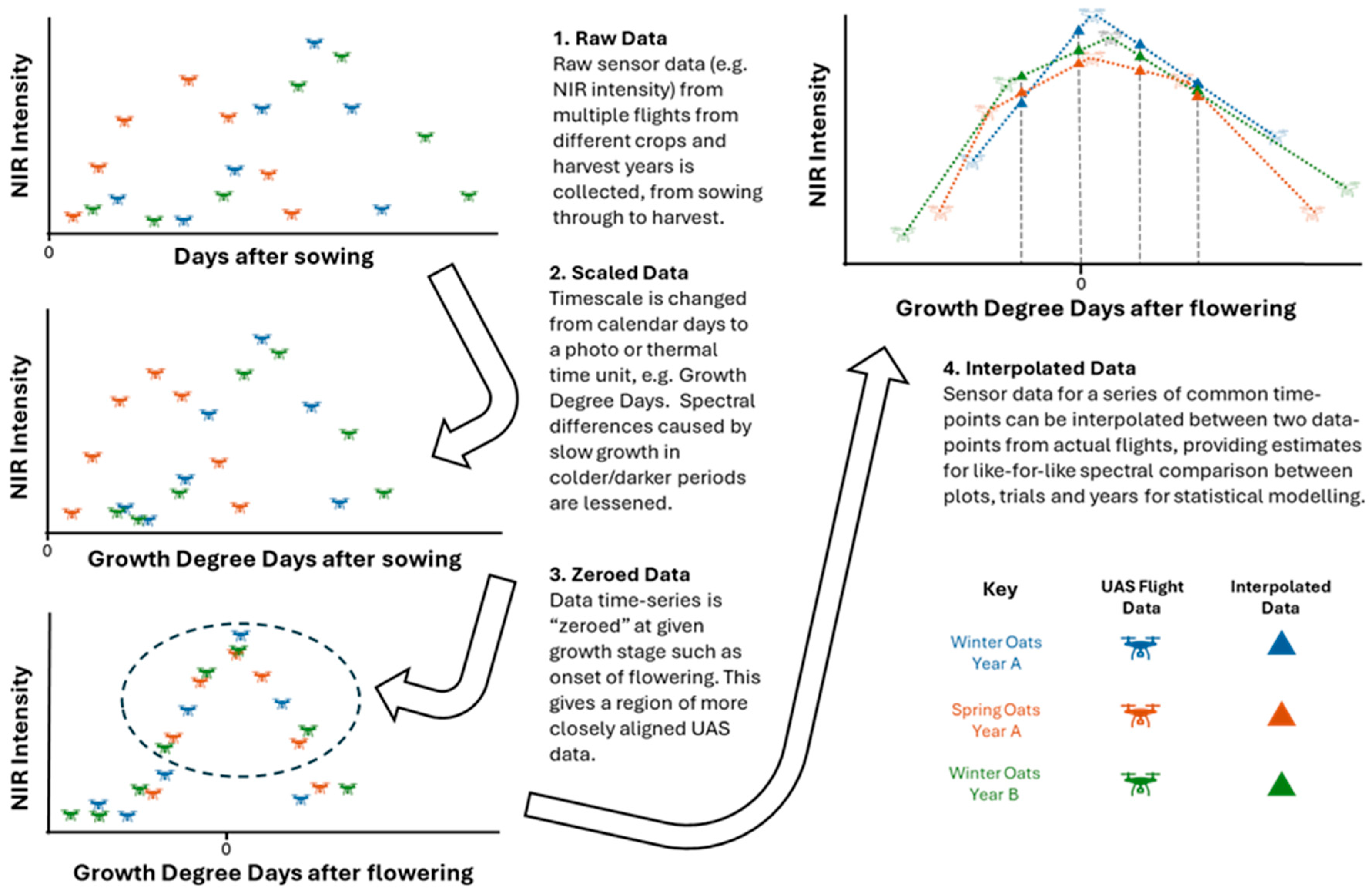
2.2. UAS Data Acquisition and Pre-Processing
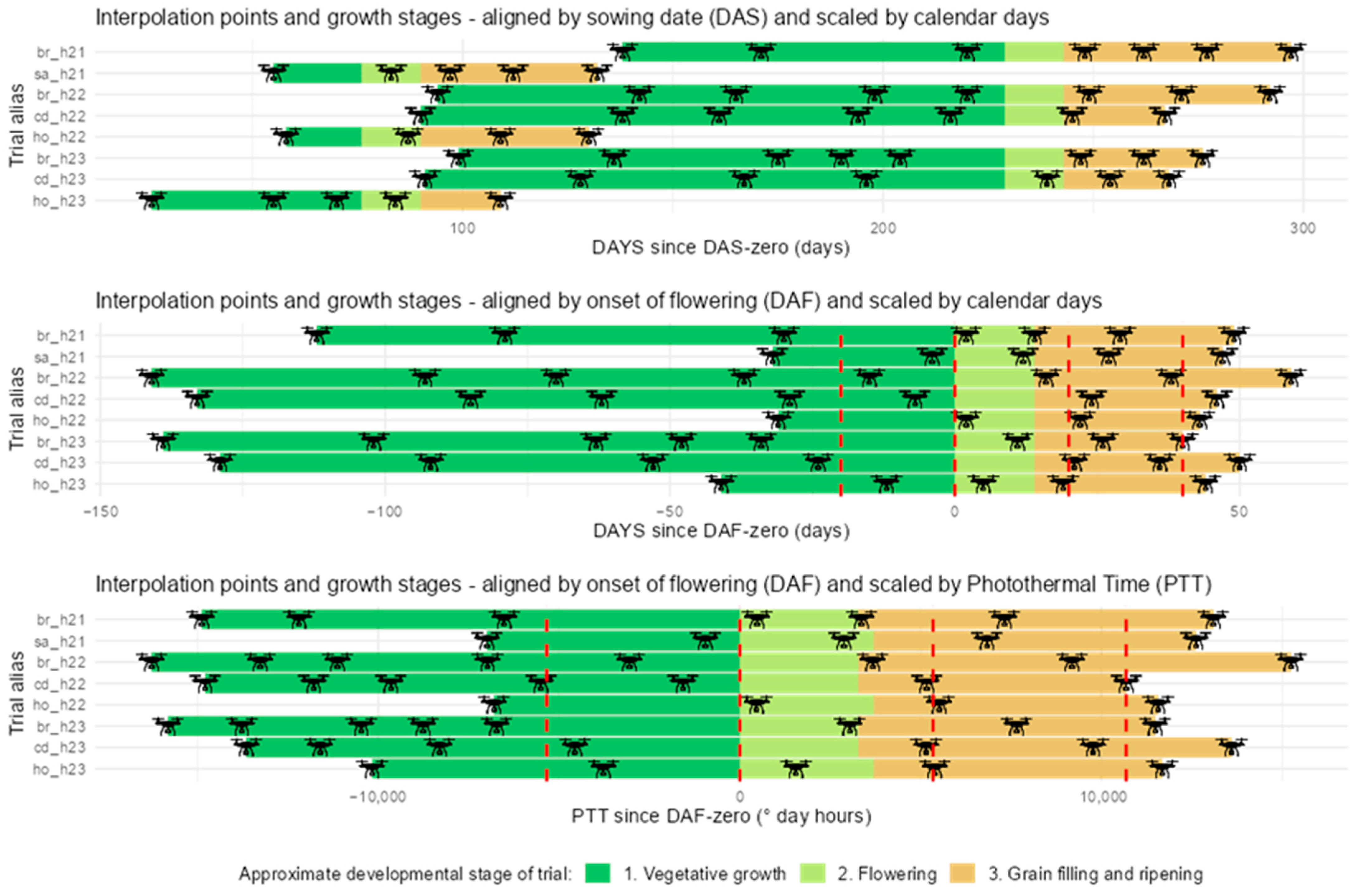
2.3. Environmental Data and Photothermal Units
2.4. Statistical Analysis
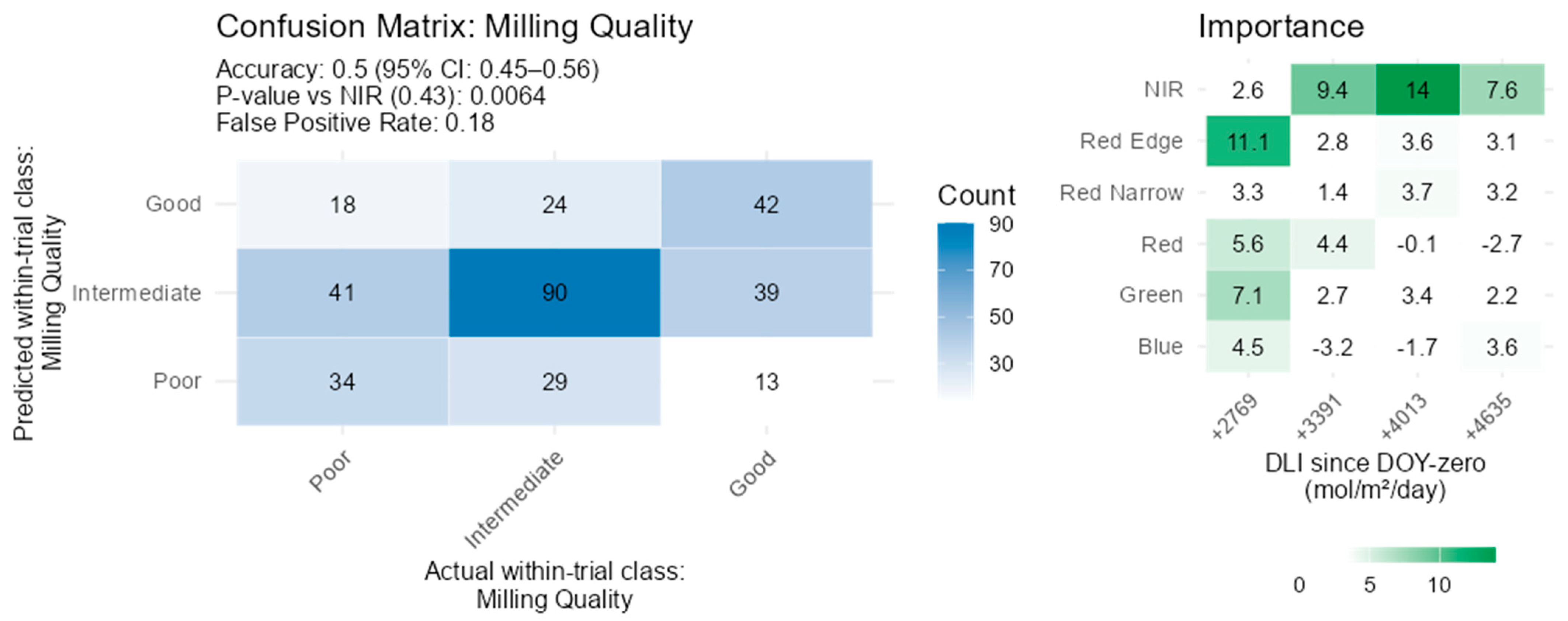
- Milling quality, which was assigned “good” if that plot yielded grain with high classifications for both kernel content and hullability, and “poor” if both kernel content and hullability were classed as low. Any other combinations were classed as “intermediate”.
- Physical quality, which was assigned “good” if both test weight and TGW classifications for the plot were high and screenings were low, and “poor” if both test weight and TGW were low and screenings high. Any other combinations were classed as “intermediate”.
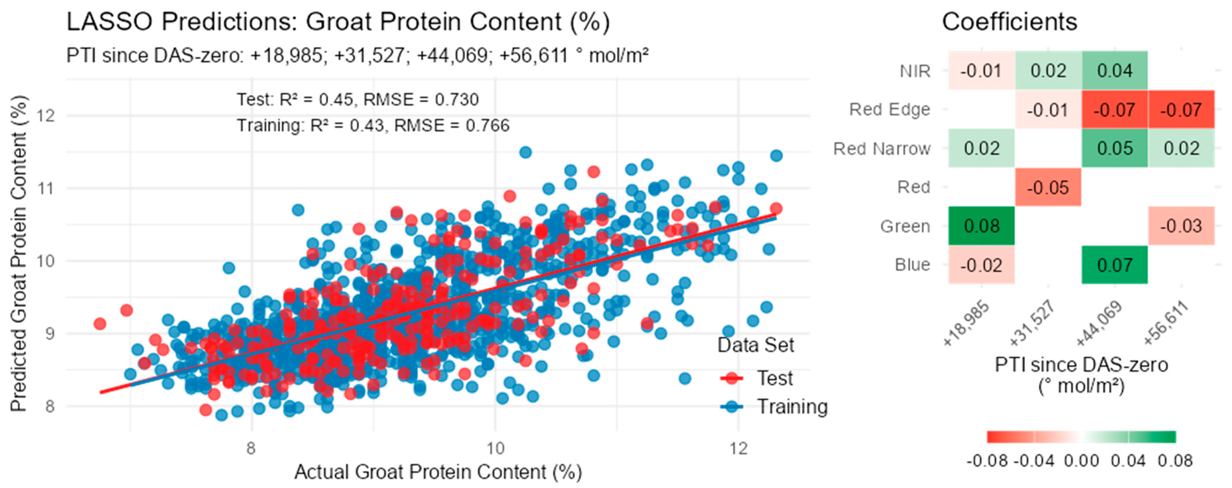
- Groat composition, which was assigned “good” if both groat protein and ß-glucan content classes were high and oil content class was low. Groat composition was classified as “poor” when both groat protein and β-glucan content classes were low and the oil content class was high. Any other combinations were classed as “intermediate”.
3. Results
3.1. Data Interpolations
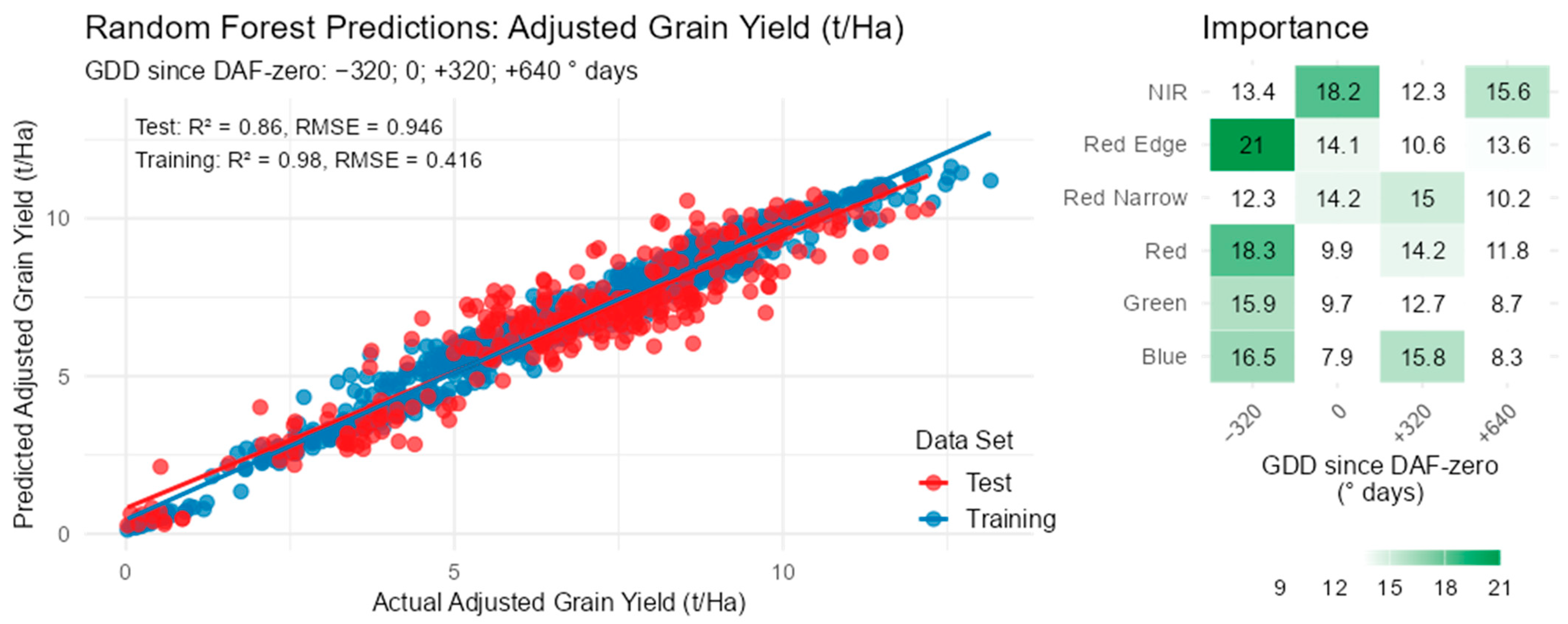
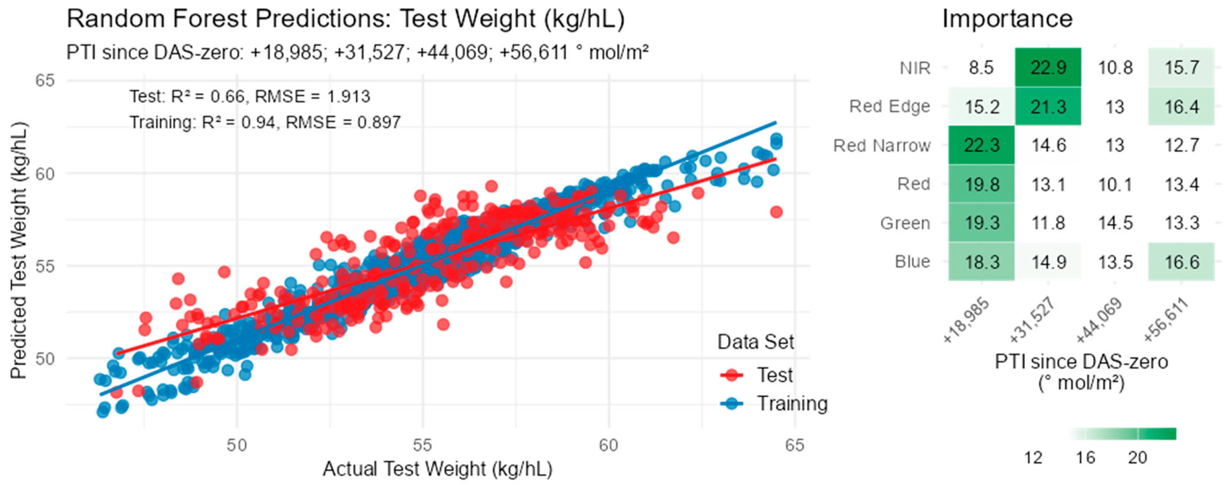
3.2. Regression Models
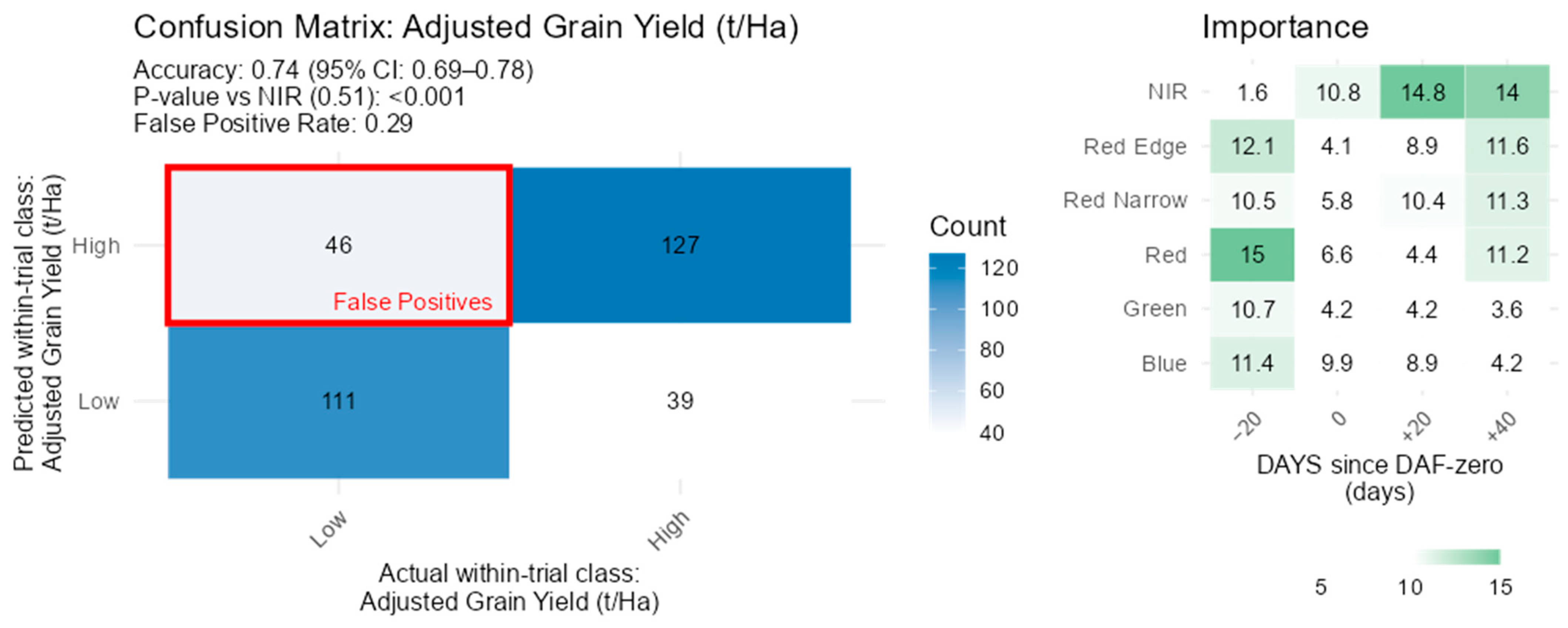
3.3. Classification Models
3.4. Grain Yield
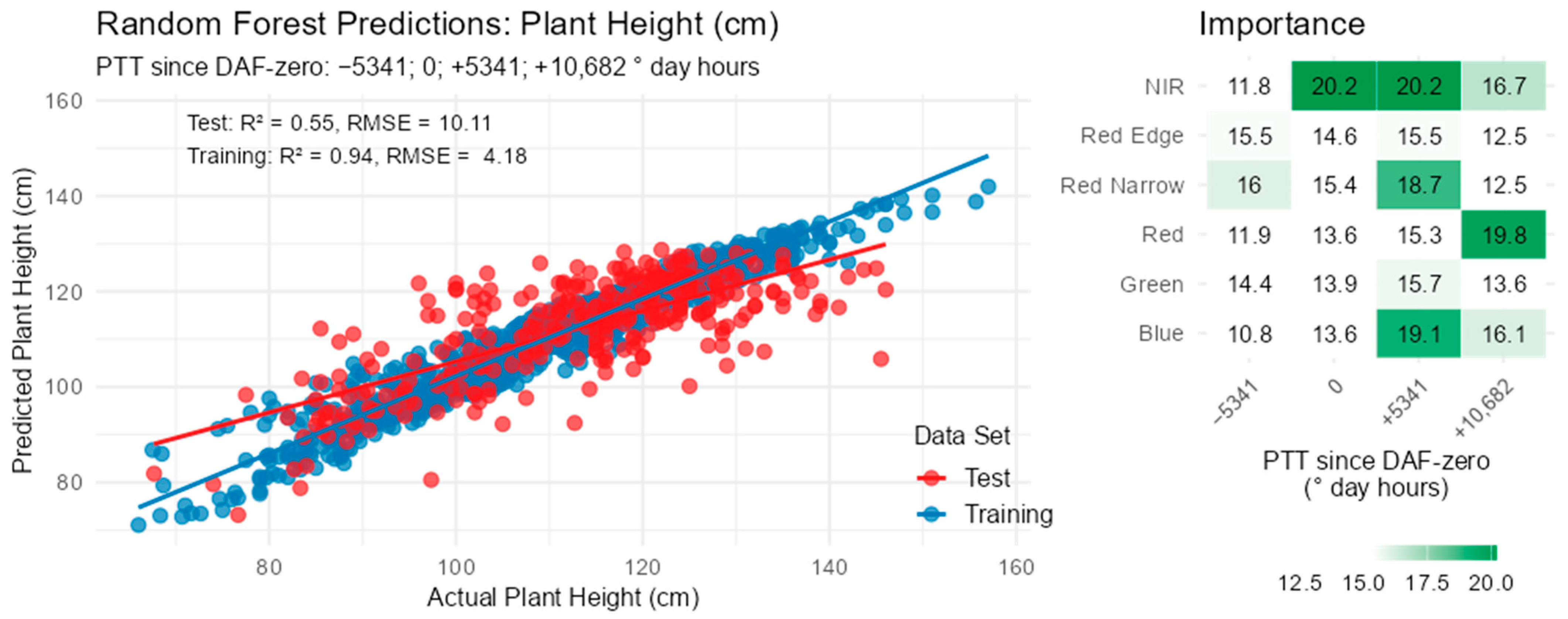
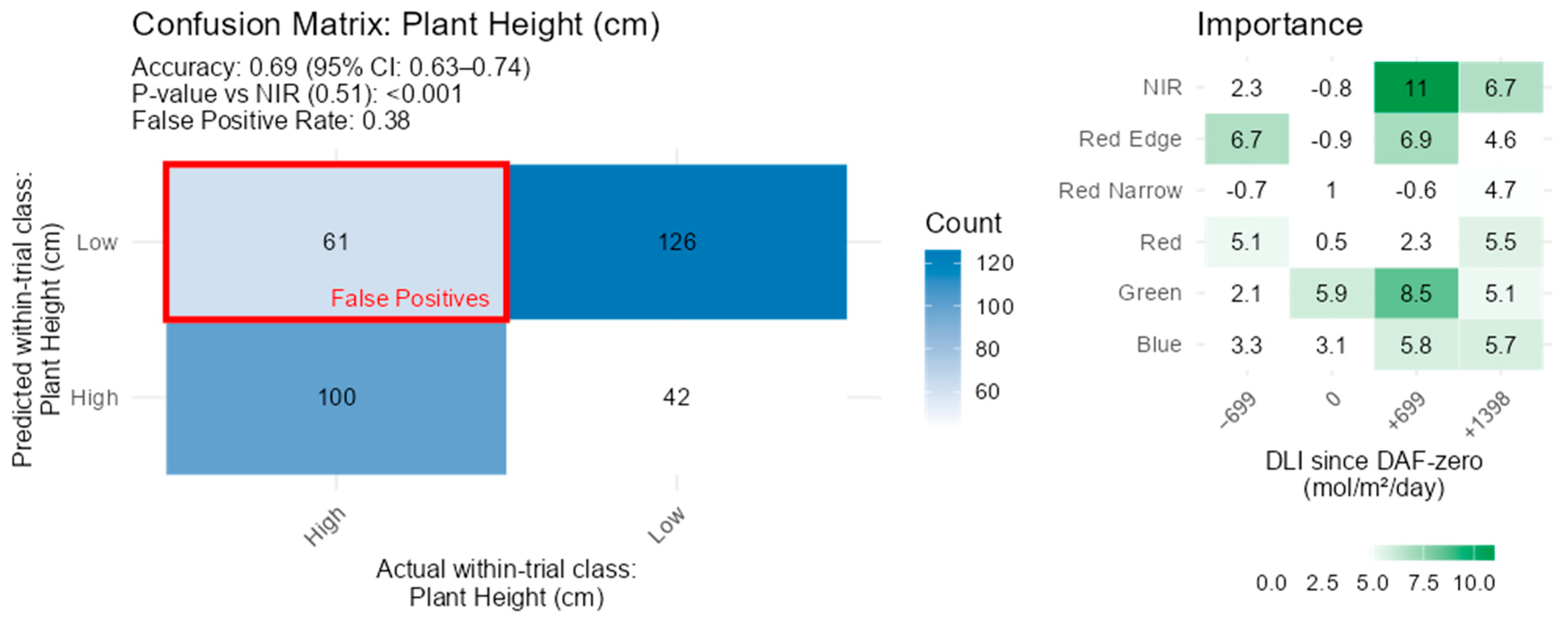
3.5. Plant Height
3.6. Milling Quality
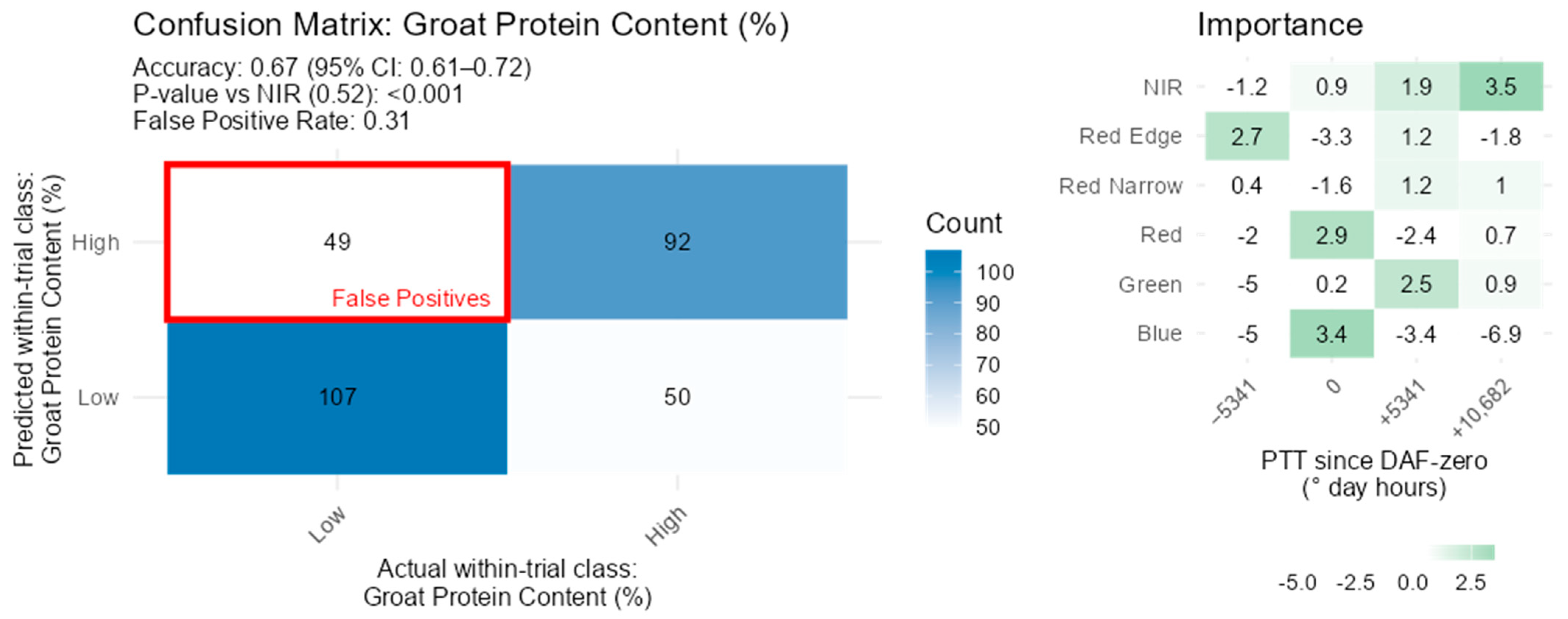
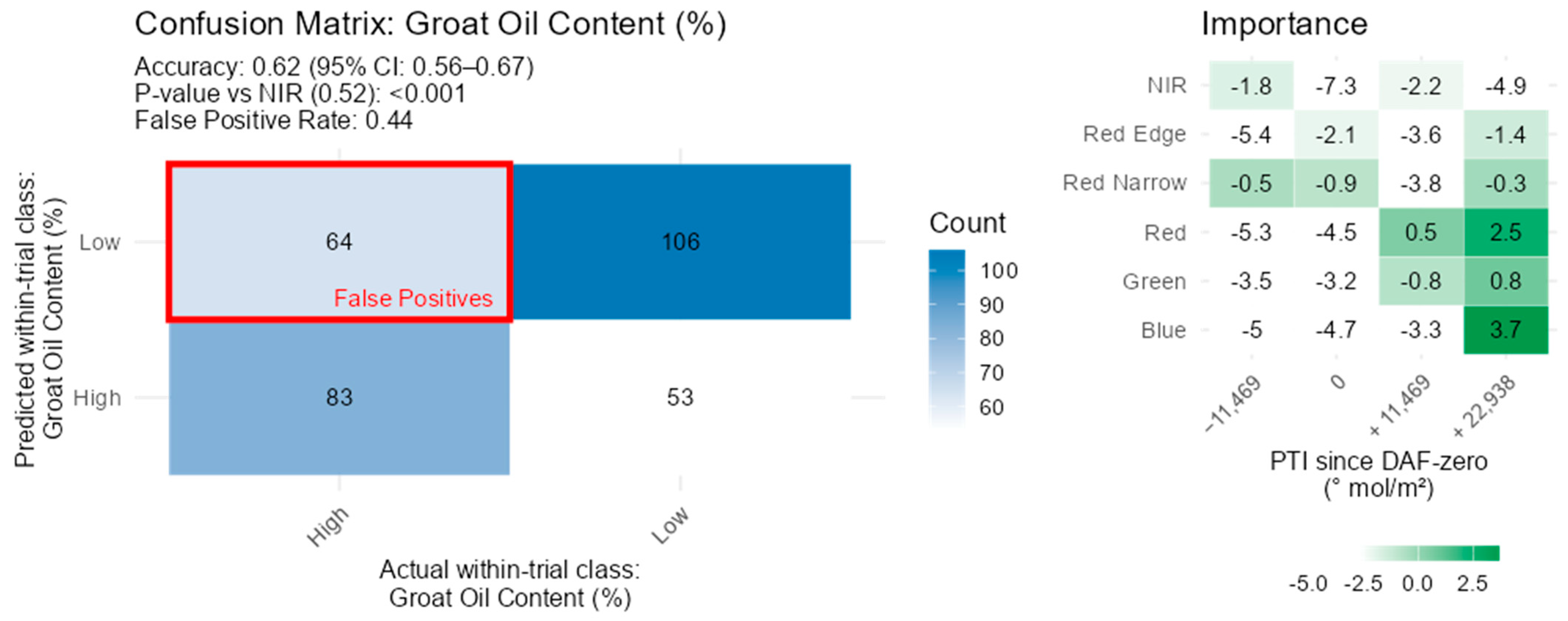
3.7. Groat Composition
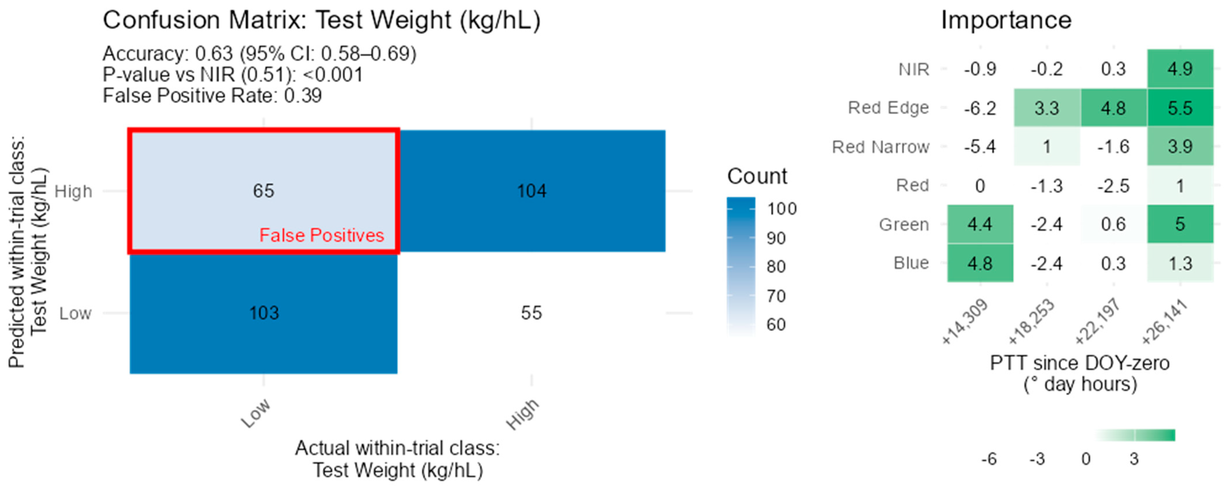
3.8. Physical Grain Quality
3.9. Ablation Study
4. Discussion
5. Conclusions
Supplementary Materials
Author Contributions
Funding
Data Availability Statement
Acknowledgments
Conflicts of Interest
References
- Brown, J.; Caligari, P.D.S.; Campos, H.A. Plant Breeding, 2nd ed.; John Wiley & Sons Ltd.: Hoboken, NJ, USA, 2014. [Google Scholar]
- Fiorani, F.; Schurr, U. Future scenarios for plant phenotyping. Annu. Rev. Plant Biol. 2013, 64, 267–291. [Google Scholar] [CrossRef] [PubMed]
- Pieruschka, R.; Schurr, U. Plant Phenotyping: Past, Present, and Future. Plant Phenomics 2019, 2019, 7507131. [Google Scholar] [CrossRef] [PubMed]
- Yang, W.; Feng, H.; Zhang, X.; Zhang, J.; Doonan, J.H.; Batchelor, W.D.; Xiong, L.; Yan, J. Crop Phenomics and High-Throughput Phenotyping: Past Decades, Current Challenges, and Future Perspectives. Mol. Plant 2020, 13, 187–214. [Google Scholar] [CrossRef] [PubMed]
- Atefi, A.; Ge, Y.; Pitla, S.; Schnable, J. Robotic Technologies for High-Throughput Plant Phenotyping: Contemporary Reviews and Future Perspectives. Front. Plant Sci. 2021, 12, 611940. [Google Scholar] [CrossRef]
- Shakoor, N.; Lee, S.; Mockler, T.C. High throughput phenotyping to accelerate crop breeding and monitoring of diseases in the field. Curr. Opin. Plant Biol. 2017, 38, 184–192. [Google Scholar] [CrossRef]
- Kris-Etherton, P.; Khoo, C.S.; Chu, Y.F. Introduction: Oat Nutrition, Health, and the Potential Threat of a Declining Production on Consumption. In Oats Nutrition and Technology; Wiley-Blackwell: Hoboken, NJ, USA, 2013; pp. 1–6. [Google Scholar] [CrossRef]
- Strychar, R. Chapter 1: World Oat Production, Trade, and Usage. In OATS: Chemistry and Technology; Cereals & Grains Association: Saint Paul, MN, USA, 2011; pp. 1–10. [Google Scholar] [CrossRef]
- Stewart, D.; McDougall, G. Oat agriculture, cultivation and breeding targets: Implications for human nutrition and health. Br. J. Nutr. 2014, 112 (Suppl. S2), S50–S57. [Google Scholar] [CrossRef]
- Gorash, A.; Armonienė, R.; Fetch, J.M.; Liatukas, Ž.; Danytė, V. Aspects in oat breeding: Nutrition quality, nakedness and disease resistance, challenges and perspectives. Ann. Appl. Biol. 2017, 171, 281–302. [Google Scholar] [CrossRef]
- Cooper, L.; Elser, J.; Laporte, M.A.; Arnaud, E.; Jaiswal, P. Planteome 2024 Update: Reference Ontologies and Knowledgebase for Plant Biology. Nucleic Acids Res. 2024, 52, D1548–D1555. [Google Scholar] [CrossRef]
- Cooper, L.; Meier, A.; Laporte, M.A.; Elser, J.L.; Mungall, C.; Sinn, B.T.; Cavaliere, D.; Carbon, S.; Dunn, N.A.; Smith, B.; et al. The Planteome database: An integrated resource for reference ontologies, plant genomics and phenomics. Nucleic Acids Res. 2018, 46, D1168–D1180. [Google Scholar] [CrossRef]
- Morales, N.; Ogbonna, A.C.; Ellerbrock, B.J.; Bauchet, G.J.; Tantikanjana, T.; Tecle, I.Y.; Powell, A.F.; Lyon, D.; Menda, N.; Simoes, C.C.; et al. Breedbase: A digital ecosystem for modern plant breeding. G3 Genes Genomes Genet. 2022, 12, jkac078. [Google Scholar] [CrossRef]
- Xie, C.; Yang, C. A review on plant high-throughput phenotyping traits using UAV-based sensors. Comput. Electron. Agric. 2020, 178, 105731. [Google Scholar] [CrossRef]
- Tanaka, T.S.T.; Wang, S.; Jørgensen, J.R.; Gentili, M.; Vidal, A.Z.; Mortensen, A.K.; Acharya, B.S.; Beck, B.D.; Gislum, R. Review of Crop Phenotyping in Field Plot Experiments Using UAV-Mounted Sensors and Algorithms. Drones 2024, 8, 212. [Google Scholar] [CrossRef]
- Yang, G.; Liu, J.; Zhao, C.; Li, Z.; Huang, Y.; Yu, H.; Xu, B.; Yang, X.; Zhu, D.; Zhang, X.; et al. Unmanned aerial vehicle remote sensing for field-based crop phenotyping: Current status and perspectives. Front. Plant Sci. 2017, 8, 1111. [Google Scholar] [CrossRef] [PubMed]
- Huang, S.; Tang, L.; Hupy, J.P.; Wang, Y.; Shao, G. A commentary review on the use of normalized difference vegetation index (NDVI) in the era of popular remote sensing. J. For. Res. 2021, 32, 1–6. [Google Scholar] [CrossRef]
- Farag, F.; Huggins, T.D.; Edwards, J.D.; McClung, A.M.; Hashem, A.A.; Causey, J.L.; Bellis, E.S. Manifold and spatiotemporal learning on multispectral unoccupied aerial system imagery for phenotype prediction. Plant Phenome J. 2024, 7, e70006. [Google Scholar] [CrossRef]
- Yuan, J.; Zhang, Y.; Zheng, Z.; Yao, W.; Wang, W.; Guo, L. Grain Crop Yield Prediction Using Machine Learning Based on UAV Remote Sensing: A Systematic Literature Review. Drones 2024, 8, 559. [Google Scholar] [CrossRef]
- Wei, L.; Yang, H.; Niu, Y.; Zhang, Y.; Xu, L.; Chai, X. Wheat biomass, yield, and straw-grain ratio estimation from multi-temporal UAV-based RGB and multispectral images. Biosyst. Eng. 2023, 234, 187–205. [Google Scholar] [CrossRef]
- Yu, J.; Cheng, T.; Cai, N.; Zhou, X.-G.; Diao, Z.; Wang, T.; Du, S.; Liang, D.; Zhang, D. Wheat Lodging Segmentation Based on Lstm_PSPNet Deep Learning Network. Drones 2023, 7, 143. [Google Scholar] [CrossRef]
- Wang, Y.; Feng, L.; Sun, W.; Wang, L.; Yang, G.; Chen, B. A lightweight CNN-Transformer network for pixel-based crop mapping using time-series Sentinel-2 imagery. Comput. Electron. Agric. 2024, 226, 109370. [Google Scholar] [CrossRef]
- Li, Z.; Chen, G.; Zhang, T. A CNN-Transformer Hybrid Approach for Crop Classification Using Multitemporal Multisensor Images. IEEE J. Sel. Top. Appl. Earth Obs. Remote Sens. 2020, 13, 847–858. [Google Scholar] [CrossRef]
- Zhang, S.; Qi, X.; Duan, J.; Yuan, X.; Zhang, H.; Feng, W.; Guo, T.; He, L. Comparison of Attention Mechanism-Based Deep Learning and Transfer Strategies for Wheat Yield Estimation Using Multisource Temporal Drone Imagery. IEEE Trans. Geosci. Remote Sens. 2024, 62, 4407723. [Google Scholar] [CrossRef]
- Yadav, S.A.; Zhang, X.; Wijewardane, N.K.; Feldman, M.; Qin, R.; Huang, Y.; Samiappan, S.; Young, W.; Tapia, F.G. Context-Aware Deep Learning Model for Yield Prediction in Potato Using Time-Series UAS Multispectral Data. IEEE J. Sel. Top. Appl. Earth Obs. Remote Sens. 2025, 18, 6096–6115. [Google Scholar] [CrossRef]
- Pichler, M.; Hartig, F. Machine learning and deep learning—A review for ecologists. Methods Ecol. Evol. 2023, 14, 994–1016. [Google Scholar] [CrossRef]
- Ahmed, S.F.; Alam, M.S.B.; Hassan, M.; Rozbu, M.R.; Ishtiak, T.; Rafa, N.; Mofijur, M.; Ali, A.B.M.S.; Gandomi, A.H. Deep learning modelling techniques: Current progress, applications, advantages, and challenges. Artif. Intell. Rev. 2023, 56, 13521–13617. [Google Scholar] [CrossRef]
- Lecun, Y.; Bengio, Y.; Hinton, G. Deep learning. Nature 2015, 521, 436–444. [Google Scholar] [CrossRef]
- Drones|UK Civil Aviation Authority. Available online: https://www.caa.co.uk/drones/ (accessed on 25 March 2025).
- The Growth Stages of Cereals|AHDB. Available online: https://ahdb.org.uk/knowledge-library/the-growth-stages-of-cereals (accessed on 9 May 2025).
- Parent, B.; Millet, E.J.; Tardieu, F. The use of thermal time in plant studies has a sound theoretical basis provided that confounding effects are avoided. J. Exp. Bot. 2019, 70, 2359–2370. [Google Scholar] [CrossRef]
- Schoving, C.; Stöckle, C.O.; Colombet, C.; Champolivier, L.; Debaeke, P.; Maury, P. Combining Simple Phenotyping and Photothermal Algorithm for the Prediction of Soybean Phenology: Application to a Range of Common Cultivars Grown in Europe. Front. Plant Sci. 2020, 10, 1755. [Google Scholar] [CrossRef]
- Poorter, H.; Fiorani, F.; Pieruschka, R.; Wojciechowski, T.; van der Putten, W.H.; Kleyer, M.; Schurr, U.; Postma, J. Pampered inside, pestered outside? Differences and similarities between plants growing in controlled conditions and in the field. New Phytol. 2016, 212, 838–855. [Google Scholar] [CrossRef]
- Segarra, J.; Rezzouk, F.Z.; Aparicio, N.; González-Torralba, J.; Aranjuelo, I.; Gracia-Romero, A.; Araus, J.L.; Kefauver, S.C. Multiscale assessment of ground, aerial and satellite spectral data for monitoring wheat grain nitrogen content. Inf. Process. Agric. 2023, 10, 504–522. [Google Scholar] [CrossRef]
- Li, Z.; Zhao, Y.; Taylor, J.; Gaulton, R.; Jin, X.; Song, X.; Li, Z.; Meng, Y.; Chen, P.; Feng, H.; et al. Comparison and transferability of thermal, temporal and phenological-based in-season predictions of above-ground biomass in wheat crops from proximal crop reflectance data. Remote Sens. Environ. 2022, 273, 112967. [Google Scholar] [CrossRef]
- Zeng, L.; Wardlow, B.D.; Wang, R.; Shan, J.; Tadesse, T.; Hayes, M.J.; Li, D. A hybrid approach for detecting corn and soybean phenology with time-series MODIS data. Remote Sens. Environ. 2016, 181, 237–250. [Google Scholar] [CrossRef]
- Prey, L.; Hanemann, A.; Ramgraber, L.; Seidl-Schulz, J.; Noack, P.O. UAV-Based Estimation of Grain Yield for Plant Breeding: Applied Strategies for Optimizing the Use of Sensors, Vegetation Indices, Growth Stages, and Machine Learning Algorithms. Remote Sens. 2022, 14, 6345. [Google Scholar] [CrossRef]
- AHDB Recommended Lists for Cereals and Oilseeds (2021–2026)|AHDB. Available online: https://ahdb.org.uk/ahdb-recommended-lists-for-cereals-and-oilseeds-2021-2026 (accessed on 9 April 2025).
- Howarth, C.J.; Martinez-Martin, P.M.J.; Cowan, A.A.; Griffiths, I.M.; Sanderson, R.; Lister, S.J.; Langdon, T.; Clarke, S.; Fradgley, N.; Marshall, A.H. Genotype and environment affect the grain quality and yield of winter oats (Avena sativa L.). Foods 2021, 10, 2356. [Google Scholar] [CrossRef]
- Chen, C.J.; Zhang, Z. GRID: A Python Package for Field Plot Phenotyping Using Aerial Images. Remote Sens. 2020, 12, 1697. [Google Scholar] [CrossRef]
- Met Office DataPoint—Met Office. Available online: https://www.metoffice.gov.uk/services/data/datapoint (accessed on 8 April 2025).
- McWilliam, S.C.; Sylvester-Bradley, R. Oat Growth Guide. 2019. Available online: https://www.hutton.ac.uk/sites/default/files/files/publications/Oat-Growth-Guide.pdf (accessed on 8 April 2025).
- McMaster, G.S.; Wilhelm, W.W. Growing degree-days: One equation, two interpretations. Agric. For. Meteorol. 1997, 87, 291–300. [Google Scholar] [CrossRef]
- Table of Sunrise/Sunset, Moonrise/Moonset, or Twilight Times for an Entire Year. Available online: https://aa.usno.navy.mil/data/RS_OneYear (accessed on 7 April 2025).
- Nandini, K.M.; Sridhara, S.; Kumar, K. Effect of different planting density on thermal time use efficiencies and productivity of guar genotypes under southern transition zone of Karnataka. J. Pharmacogn. Phytochem. 2019, 8, 2092–2097. Available online: https://www.phytojournal.com/archives/2019.v8.i1.7076/effect-of-different-planting-density-on-thermal-time-use-efficiencies-and-productivity-of-guar-genotypes-under-southern-transition-zone-of-karnataka (accessed on 8 April 2025).
- CAMS Solar Radiation Time-Series. Copernicus Atmosphere Monitoring Service (CAMS) Atmosphere Data Store (ADS). Available online: https://ads.atmosphere.copernicus.eu/datasets/cams-solar-radiation-timeseries?tab=overview (accessed on 7 April 2025).
- Schroedter-Homscheidt, M.; Azam, F.; Betcke, J.; Hanrieder, N.; Lefèvre, M.; Saboret, L.; Saint-Drenan, Y.-M. Surface solar irradiation retrieval from MSG/SEVIRI based on APOLLO Next Generation and HELIOSAT 4 methods. Meteorol. Z. 2022, 31, 455–476. [Google Scholar] [CrossRef]
- Qu, Z.; Oumbe, A.; Blanc, P.; Espinar, B.; Gesell, G.; Gschwind, B.; Klüser, L.; Lefèvre, M.; Saboret, L.; Schroedter-Homscheidt, M.; et al. Fast radiative transfer parameterisation for assessing the surface solar irradiance: The Heliosat 4 method. Meteorol. Z. 2017, 26, 33–57. [Google Scholar] [CrossRef]
- Gschwind, B.; Wald, L.; Blanc, P.; Lefèvre, M.; Schroedter-Homscheidt, M.; Arola, A. Improving the McClear model estimating the downwelling solar radiation at ground level in cloud-free conditions—McClear v3. Meteorol. Z. 2019, 28, 147–163. [Google Scholar] [CrossRef]
- Lefèvre, M.; Oumbe, A.; Blanc, P.; Espinar, B.; Gschwind, B.; Qu, Z.; Wald, L.; Schroedter-Homscheidt, M.; Hoyer-Klick, C.; Arola, A.; et al. McClear: A new model estimating downwelling solar radiation at ground level in clear-sky conditions. Atmos. Meas. Tech. 2013, 6, 2403–2418. [Google Scholar] [CrossRef]
- McCree, K.J. The action spectrum, absorptance and quantum yield of photosynthesis in crop plants. Agric. Meteorol. 1971, 9, 191–216. [Google Scholar] [CrossRef]
- Spitters, C.J.T.; Toussaint, H.A.J.M.; Goudriaan, J. Separating the diffuse and direct component of global radiation and its implications for modeling canopy photosynthesis Part I. Components of incoming radiation. Agric. For. Meteorol. 1986, 38, 217–229. [Google Scholar] [CrossRef]
- Nyamsi, W.W.; Espinar, B.; Blanc, P.; Wald, L. Estimating the photosynthetically active radiation under clear skies by means of a new approach. Adv. Sci. Res. 2015, 12, 5–10. [Google Scholar] [CrossRef]
- García-Rodríguez, A.; García-Rodríguez, S.; Díez-Mediavilla, M.; Alonso-Tristán, C. Photosynthetic Active Radiation, Solar Irradiance and the CIE Standard Sky Classification. Appl. Sci. 2020, 10, 8007. [Google Scholar] [CrossRef]
- Thimijan, R.W.; Heins, R.D.; Thimijan, R.W.; Heins, R.D. Photometric, Radiometric, and Quantum Light Units of Measure: A Review of Procedures for Interconversion. HortScience 1983, 18, 818–822. [Google Scholar] [CrossRef]
- Sager, J.C.; McFarlane, J.C. Radiation. In NorthCentral Regional Research Publication; Iowa State University: Ames, IA, USA, 1997. [Google Scholar]
- Kuhn, M. Building Predictive Models in R Using the caret Package. J. Stat. Softw. 2008, 28, 1–26. [Google Scholar] [CrossRef]
- Friedman, J.; Hastie, T.; Tibshirani, R. Regularization Paths for Generalized Linear Models via Coordinate Descent. J. Stat. Softw. 2010, 33, 1–22. [Google Scholar] [CrossRef]
- Tay, J.K.; Narasimhan, B.; Hastie, T. Elastic Net Regularization Paths for All Generalized Linear Models. J. Stat. Softw. 2023, 106, 1–31. [Google Scholar] [CrossRef]
- Breiman, L. Random forests. Mach. Learn. 2001, 45, 5–32. [Google Scholar] [CrossRef]
- Silva, M.L.; da Silva, A.R.A.; de Moura Neto, J.M.; Calou, V.B.C.; Fernandes, C.N.V.; Araújo, E.M. Enhanced Water Monitoring and Corn Yield Prediction Using Rpa-Derived Imagery. Eng. Agríc. 2025, 45, e20240092. [Google Scholar] [CrossRef]
- Choroś, T.; Oberski, T.; Kogut, T. UAV imaging at RGB for crop condition monitoring. Int. Arch. Photogramm. Remote Sens. Spat. Inf. Sci.—ISPRS Arch. 2020, 43, 1521–1525. [Google Scholar] [CrossRef]
- Thapa, S.; Rudd, J.C.; Xue, Q.; Bhandari, M.; Reddy, S.K.; Jessup, K.E.; Liu, S.; Devkota, R.N.; Baker, J.; Baker, S. Use of NDVI for characterizing winter wheat response to water stress in a semi-arid environment. J. Crop Improv. 2019, 33, 633–648. [Google Scholar] [CrossRef]
- Sharma, N.; Kumar, M.; Daetwyler, H.D.; Trethowan, R.M.; Hayden, M.; Kant, S. Phenotyping for heat stress tolerance in wheat population using physiological traits, multispectral imagery, and machine learning approaches. Plant Stress 2024, 14, 100593. [Google Scholar] [CrossRef]
- Descals, A.; Torres, K.; Verger, A.; Peñuelas, J. Evaluating Sentinel-2 for Monitoring Drought-Induced Crop Failure in Winter Cereals. Remote Sens. 2025, 17, 340. [Google Scholar] [CrossRef]
- Mahlein, A.K. Plant disease detection by imaging sensors—Parallels and specific demands for precision agriculture and plant phenotyping. Plant Dis. 2016, 100, 241–254. [Google Scholar] [CrossRef]

| Trait | Crop Ontology Trait ID | Description | Breeding Target for UK Milling Oats |
|---|---|---|---|
| Plant Height (cm) | CO_350:0000232 | Height of plant from the ground to tip of the panicle | Decrease (plants with short, stiff straw desirable) |
| Grain Yield (t/ha) | CO_350:0000260 | Total weight of grains harvested per unit area | Increase |
| Kernel Content (%) | CO_350:0000162 | Percentage weight of harvested grain attributed to the valuable oat kernel/groat rather than the less valuable fibrous husk (which is removed during processing) | Increase |
| Hullability (%) | CO_350:0005066 | Weight of seed that is effectively dehulled via a standardised mechanical process as a percentage of the total weight of the sample | Increase |
| Screenings (%) | n/a | Percentage weight of harvested grain that is less than 2.0 mm in width | Decrease (plump, round, and uniformly sized grains desirable) |
| Specific Weight (kg/hL) | CO_350:0000259 | Measurement of the weight of grain per unit volume | Increase |
| Thousand Grain Weight (g, as-is) | CO_350:0000251 | Weight of 1000 representative whole grains | Increase |
| Beta-glucan Content (%) | CO_350:0005065 | Amount of beta-glucan present in the groat expressed as a percentage of the entire groat weight | Increase |
| Protein Content (%) | CO_350:0000164 | The amount of protein in the groat, expressed as a percentage of the groat weight | Increase |
| Oil Content (%) | CO_350:0000163 | The amount of oil in the groat, expressed as a percentage of the groat weight | Decrease |
| Trial Alias | Harvest Year | Crop | Trial Type | Sowing Date | Total Plots |
|---|---|---|---|---|---|
| br_h21 | 2021 | Winter Oats | Commercial advanced breeding lines | Week 41, 2020 | 395 |
| sa_h21 | 2021 | Spring Oats | Nitrogen response trial, commercial varieties | Week 12, 2021 | 54 |
| br_h22 | 2022 | Winter Oats | Commercial advanced breeding lines | Week 40, 2021 | 393 |
| cd_h22 | 2022 | Facultative Oats | Mixed commercial varieties and advanced breeding lines | Week 41, 2021 | 300 |
| ho_h22 | 2022 | Spring Oats | Mixed commercial and heritage varieties | Week 12, 2022 | 75 |
| br_h23 | 2023 | Winter Oats | Commercial crosses for breeding programmes | Week 41, 2022 | 393 |
| cd_h23 | 2023 | Facultative Oats | Mixed commercial varieties and advanced breeding lines | Week 42, 2022 | 300 |
| ho_h23 | 2023 | Spring Oats | Mixed commercial varieties and advanced breeding lines | Week 16, 2023 | 75 |
| Removed Sensor | Average Difference from Fully Trained Model | ||
|---|---|---|---|
| LASSO Regression R2 | Random Forest Regression R2 | Random Forest Classification Accuracy (%) | |
| Red | −0.004 *** | −0.002 *** | −0.08 ns |
| Green | −0.005 *** | −0.001 ns | 0.05 ns |
| Blue | −0.011 *** | −0.009 *** | −0.79 *** |
| Red Narrow | −0.010 *** | −0.004 *** | −0.36 ns |
| Reg Edge | −0.012 *** | −0.002 *** | −0.58 ** |
| NIR | −0.015 *** | −0.013 *** | −0.99 *** |
Disclaimer/Publisher’s Note: The statements, opinions and data contained in all publications are solely those of the individual author(s) and contributor(s) and not of MDPI and/or the editor(s). MDPI and/or the editor(s) disclaim responsibility for any injury to people or property resulting from any ideas, methods, instructions or products referred to in the content. |
© 2025 by the authors. Licensee MDPI, Basel, Switzerland. This article is an open access article distributed under the terms and conditions of the Creative Commons Attribution (CC BY) license (https://creativecommons.org/licenses/by/4.0/).
Share and Cite
Evershed, D.; Brook, J.; Cowan, S.; Griffiths, I.; Tudor, S.; Loosley, M.; Doonan, J.H.; Howarth, C.J. Photothermal Integration of Multi-Spectral Imaging Data via UAS Improves Prediction of Target Traits in Oat Breeding Trials. Agronomy 2025, 15, 1583. https://doi.org/10.3390/agronomy15071583
Evershed D, Brook J, Cowan S, Griffiths I, Tudor S, Loosley M, Doonan JH, Howarth CJ. Photothermal Integration of Multi-Spectral Imaging Data via UAS Improves Prediction of Target Traits in Oat Breeding Trials. Agronomy. 2025; 15(7):1583. https://doi.org/10.3390/agronomy15071583
Chicago/Turabian StyleEvershed, David, Jason Brook, Sandy Cowan, Irene Griffiths, Sara Tudor, Marc Loosley, John H. Doonan, and Catherine J. Howarth. 2025. "Photothermal Integration of Multi-Spectral Imaging Data via UAS Improves Prediction of Target Traits in Oat Breeding Trials" Agronomy 15, no. 7: 1583. https://doi.org/10.3390/agronomy15071583
APA StyleEvershed, D., Brook, J., Cowan, S., Griffiths, I., Tudor, S., Loosley, M., Doonan, J. H., & Howarth, C. J. (2025). Photothermal Integration of Multi-Spectral Imaging Data via UAS Improves Prediction of Target Traits in Oat Breeding Trials. Agronomy, 15(7), 1583. https://doi.org/10.3390/agronomy15071583