Autonomous Navigation and Obstacle Avoidance for Orchard Spraying Robots: A Sensor-Fusion Approach with ArduPilot, ROS, and EKF

Abstract

To address the challenges of low pesticide utilization, insufficient automation, and health risks in orchard plant protection, we developed an autonomous spraying vehicle using ArduPilot firmware and a robot operating system (ROS). The system tackles orchard navigation hurdles, including global navigation satellite system (GNSS) signal obstruction, light detection and ranging (LIDAR) simultaneous localization and mapping (SLAM) error accumulation, and lighting-limited visual positioning. A key innovation is the integration of an extended Kalman filter (EKF) to dynamically fuse T265 visual odometry, inertial measurement unit (IMU), and GPS data, overcoming single-sensor limitations and enhancing positioning robustness in complex environments. Additionally, the study optimizes PID controller derivative parameters for tracked chassis, improving acceleration/deceleration control smoothness. The system, composed of Pixhawk 4, Raspberry Pi 4B, Silan S2L LIDAR, T265 visual odometry, and a Quectel EC200A 4G module, enables autonomous path planning, real-time obstacle avoidance, and multi-mission navigation. Indoor/outdoor tests and field experiments in Sun Village Orchard validated its autonomous cruising and obstacle avoidance capabilities under real-world orchard conditions, demonstrating feasibility for intelligent plant protection.

1. Introduction

Following grains and vegetables, the fruit sector has risen to become China’s third-largest cultivation industry. Orchard plant protection is a key link to ensure stable and increased fruit production. At present, orchard plant protection mainly relies on the spraying of chemical pesticides for pest control, but this method has problems such as low pesticide utilization, low degree of automation, and damage to the health of sprayers [1,2,3]. With the advancement of science and technology, orchard machinery is evolving towards automation and intelligence. Orchard robotic navigation technology enables effective implementation of pest and disease control measures. Through autonomous cruising and precision spraying, it enhances operational efficiency and quality while reducing labor intensity and costs. The current mainstream navigation methods for autonomous navigation robots include satellite positioning navigation, laser positioning navigation, and visual positioning navigation [4,5,6].

Previous studies have shown that GNSS can provide high-precision, all-weather positioning information for navigation robots in an unobstructed outdoor environment. This approach offers high positioning accuracy that can meet the localization requirements of robots [7,8,9]. Xiong et al. [10] applied the Beidou Navigation Satellite System (BDS) to the navigation of orchard spraying machines. They conducted experiments in a cherry orchard with a planting row spacing of 5 m and successfully achieved straight-line tracking, with a navigation accuracy of maximum error not exceeding 0.13 m. However, testing in densely planted orchards, where satellite signal obstruction is more likely to occur, has not yet been conducted. In recent years, LIDAR has been widely used in mobile robot autonomous navigation systems due to its high measurement accuracy, long measurement range, and ability to provide rich distance information [11]. Hu et al. [12] proposed a positioning system for agricultural robots that utilizes a two-dimensional LIDAR and laser receivers. By fusing the time difference of laser scans and point cloud features, they achieved high-precision positioning in environments with weak or no satellite signals. Experimental results demonstrated that the system can meet the requirements of automatic navigation for agricultural robots. With the increasing maturity of machine vision technology, visual sensors are widely used in the field of agricultural robots due to their advantages of rich information content and lower cost [13,14]. Adrien et al. [15] used a deep learning-based neural network model on RGB-D images. They integrated the obtained trunk data into the particle-filter localization algorithm, reducing the pre-convergence distance and time while increasing the correct convergence rate.

Due to the complexity of the orchard environment, GNSS can be obscured by tree canopies and branches, leading to inaccurate positioning [16,17]. Laser positioning navigation is prone to error accumulation, which can result in a decrease in positioning accuracy [18]. Visual positioning navigation can be limited by lighting conditions and may not meet the navigation requirements [19]. Recent studies have explored multi-sensor fusion to address these limitations: Fujinaga [20] proposed a hybrid navigation strategy switching between waypoint and bed navigation using LIDAR to maintain a distance error within ±0.05 m, but this method lacks real-time adaptability to dynamic obstacles and relies on static pre-mapped environments. Ospina and Itakura [21] developed a layered costmap system with 2D LIDAR for obstacle avoidance, achieving lateral errors of 0.15–0.28 m, yet its reliance on predefined road structures limits applicability to unstructured orchards. Jiang et al. [22] integrated 3D LIDAR SLAM with IMU and encoder data to reduce positioning errors to <16 cm, but the method struggles with dynamic obstacles due to its static map-based framework. Liu et al. [23] introduced NPENet, a lightweight neural network for real-time road centerline detection (accuracy 92.14%), but its performance declines in weed-covered or cluttered paths.

Despite these advances, multi-sensor fusion in orchards still faces three core challenges: dynamic environment adaptability (inability to handle moving obstacles or changing crop layouts), unresolved sensor heterogeneity and noise (e.g., IMU drift, visual motion blur), and high-computational-efficiency and cost-limiting small-scale farm deployment. This study addresses these gaps by proposing an autonomous cruising and obstacle avoidance system based on ArduPilot and ROS, featuring EKF-based multi-sensor fusion to dynamically combine GPS, visual odometry, and IMU data for robust positioning, adaptive obstacle avoidance via LIDAR point clouds and visual semantics with real-time path replanning, and lightweight hardware integration (e.g., Silan S2L LIDAR, Raspberry Pi 4B) validated across diverse environments.

2. Materials and Methods

2.1. Design of Autonomous Cruising and Obstacle Avoidance System

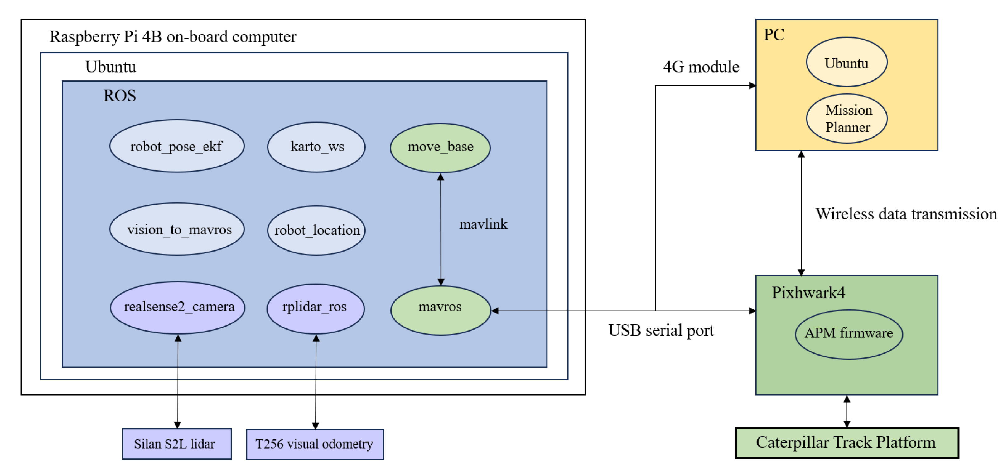
2.1.1. System Hardware Design

The system is based on the Pixhawk 4 unmanned vehicle platform and uses the Raspberry Pi 4B (Raspberry Pi Foundation, Cambridge, UK) as its onboard computer. We selected this board for its quad-core ARM Cortex A72 processor (1.5 GHz), 4 GB LPDDR4 RAM, and compatibility with Ubuntu 20.04 and ROS Noetic. Its USB 3.0 and gigabit Ethernet interfaces enable high-speed data transfer from LIDAR and visual odometry, while GPIO pins support seamless integration with Pixhawk 4 via UART communication. The system is capable of performing SLAM and path planning based on LIDAR and visual odometry. A hardware block diagram of the system is shown in Figure 1.

The system integrates Silan S2L LIDAR (SLAMTEC, Pudong New Area, Shanghai, China) and T265 visual odometry (Intel, Santa Clara, CA, USA) for real-time collection of ambient information and mileage data while employing the Quectel EC200A 4G module (QUECTEL, Minhang District, Shanghai, China) to enable IoT communication. The core controller of the system is the Pixhawk 4 (Holybro, Shenzhen, China), which utilizes the MAVROS communication protocol to exchange information with the Raspberry Pi. Additionally, the system is equipped with a RadioLink AT9S (RadioLink, Shenzhen, China) remote controller, allowing for manual control of the unmanned vehicle. The specific parameters of the sensors are shown in

Table 1. Main Technical Parameters of Sensors.

Sensor	Type	Parameters
LIDAR	Silan S2L	Scanning range: 0.1–12 m Angular resolution: 0.1125° Scan frequency: 10 Hz
Visual Odometry	Intel RealSense T265	Resolution: 848 × 800 pixels Field of view: 87 °H × 58 °V Frame rate: 30 Hz
IMU	Pixhawk 4 (ICM-20689)	Accelerometer range: ±4 g Gyroscope range: ±500°/s Frequency: 50 Hz
GPS	M9N	Accuracy: 1.5 m (CEP) Update rate: 25 Hz

.

The T256 visual odometry, Silan S2L LIDAR, and GPS work in coordination to collect environmental data, which is transmitted to the Raspberry Pi 4B for processing. The Raspberry Pi 4B fuses data from the visual odometry, LIDAR, and GPS through SLAM and path planning algorithms to generate control commands. These commands are sent to the Pixhawk 4 flight controller, driving the unmanned vehicle to perform navigation and obstacle avoidance tasks. Ground operators can establish communication links with the control system via a PC-based graphical interface or a remote controller, using either a wireless data transmission module or the Quectel EC200A 4G module, to achieve functions such as parameter configuration, mission monitoring, and emergency manual intervention.

2.1.2. System Software Design

The Pixhawk 4 is installed with the ArduPilot firmware, while the Raspberry Pi 4B is equipped with Ubuntu 20.04 Server (Canonical Ltd., Greater London, London, UK) and ROS. The system employs the Karto SLAM algorithm for mapping the environment, and utilizes the navigation package for path planning. The system achieves communication between the flight controller, Raspberry Pi, and the PC using the MAVROS communication protocol. The PC is equipped with a Mission Planner ground station and ROS. Among the ROS-based tools, Rviz and rqt play crucial roles. Rviz is used for 3D visualization of sensor data and the robot state, while rqt provides a graphical user interface for runtime monitoring and debugging. They are employed to visualize and display the unmanned vehicle’s operational status. The software architecture of the system is shown in Figure 2.

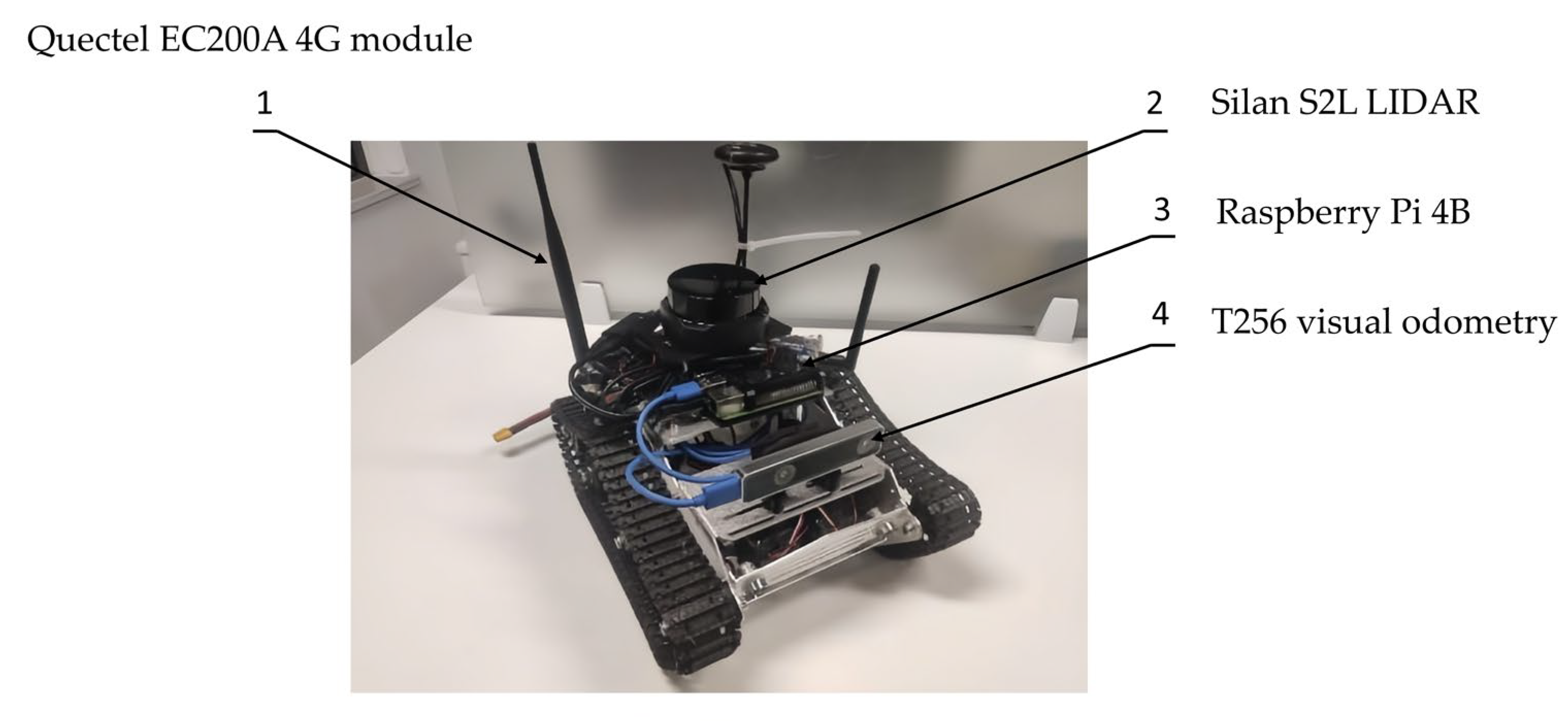
2.2. Experimental Design and Model Vehicle Construction

This study conducted multiple experiments both indoors and outdoors to validate the system’s behavior and path planning capabilities in constrained and open environments. Indoor experiments involved evaluating the system’s navigation through narrow passages, obstacle avoidance, environmental perception, and SLAM accuracy. Outdoor experiments encompassed assessing the system’s adaptability and robustness across different terrain, such as open areas, grassy terrain, uneven surfaces, and various weather conditions. By comparing and analyzing the results from indoor and outdoor experiments, this study comprehensively evaluated the system’s performance and functionality, providing an assessment of its feasibility and reliability in different scenarios and environments. The experimental design in this study contributes to ensuring the system’s stability and usability, laying a solid foundation for its practical application and deployment. The model vehicle test platform is shown in Figure 3.

The model vehicle is equipped with features such as SLAM, path planning, real-time obstacle avoidance, and outdoor autonomous cruising. The SLAM functionality enables the acquisition of localization data, which is then used in conjunction with Mission Planner on the PC to plan waypoints. These waypoints are converted into 2D goals on a costmap, facilitating global path planning. Additionally, real-time obstacle avoidance is achieved using the LIDAR and local path planning is performed using the dynamic window approach. By setting waypoints in Mission Planner, the unmanned vehicle can autonomously cruise based on the latitude and longitude coordinates of these waypoints. Moreover, by converting the latitude and longitude coordinates of the waypoints into ROS coordinates, multiple 2D goals can be planned in the costmap, enabling autonomous navigation to multiple waypoints for multi-point tasks.

2.3. Sensor Data Fusion

2.3.1. Extended Kalman Filter

The EKF [24] is a powerful algorithm widely used for state estimation in nonlinear systems. It approximates the nonlinear function through a first-order Taylor expansion, transforming the nonlinear problem into a locally linear problem, thereby enabling effective estimation of the state in complex systems. In the sensor data fusion scenario involved in this system, the EKF plays a crucial role. It can combine the advantages of different sensors to improve the accuracy of the data and the positioning performance of the system. The general equation system of the EKF is as follows.

(1)

Definition of the state vector

Let the state vector of the system be $x_k$ which is an n-dimensional vector. In different application scenarios, $x_k$ contains different state variables.

(2)

State equation

The transition of the system’s state from discrete time k to k + 1 is described by the following nonlinear state equation:

$$x_{k+1}=f(x_k,u_k,w_k)$$

(1)

where $u_k$ is the control input vector of the system with a dimension of m, that is, $u_k\in {\mathbb{R}}^m$. The meaning of the control input varies in different scenarios.

$w_k$ is the process noise vector, which follows a Gaussian distribution $w_k\sim N(0,Q_k)$, where $Q_k$ is an $n\times n$ process noise covariance matrix, reflecting the uncertainty in the state transition process.

(3)

Measurement equation

The relationship between the measurement vector $z_k$ and the system state $x_k$ is represented by the following nonlinear measurement equation:

$$z_k=h(x_k,v_k)$$

(2)

where $z_k$ is the measurement vector, with a dimension of p, that is, $z_k\in {\mathbb{R}}^p$. In different scenarios, the measurement vector can be the measured values of different sensors, such as the position measurement of a GPS, the position and attitude measurement of a visual odometer, etc.

$v_k$ is the measurement noise vector, which follows a Gaussian distribution $v_k\sim N(0,R_k)$, where $R_k$ is a $p\times p$ measurement noise covariance matrix, reflecting the uncertainty in the measurement process.

(4)

State prediction

Based on the state estimate ${\widehat{x}}_{k|k}$ at the previous moment and the control input $u_k$, the state at the current moment is predicted. The equation is as follows:

$${\widehat{x}}_{k+1|k}=f({\widehat{x}}_{k|k},u_k,0)$$

(3)

Here, the process noise is set to 0 for prediction because the state transition is predicted under ideal conditions.

(5)

Calculation of the state transition Jacobian matrix $F_k$

To linearize the nonlinear state equation, it is necessary to calculate the state transition Jacobian matrix $F_k$:

$$F_k={\left.{\displaystyle \frac{\partial f(x,u_k,0)}{\partial x}}\right|}_{x={\widehat{x}}_{k|k}}$$

(4)

$F_k$ is an $n\times n$ matrix, which describes how a small change in the state affects the state prediction at the next moment.

(6)

Covariance prediction

Based on the state transition Jacobian matrix $F_k$ and the process noise covariance matrix $Q_k$, the covariance matrix of the state estimate at the current moment is predicted:

$$P_{k+1|k}=F_k{P}_{k|k}{F}_k^T+{G_{k}Q}_k{G}_k^T$$

(5)

where $P_{k|k}$ is the covariance matrix of the state estimate at the previous moment and $P_{k+1|k}$ reflects the uncertainty of the predicted state. $G_k$ is the gain matrix of the process noise $w_k$, which describes how the process noise affects the system state.

(7)

Calculation of the measurement Jacobian matrix $H_k$

To linearize the nonlinear measurement equation, the measurement Jacobian matrix $H_k$ is calculated:

$$H_k={\displaystyle \frac{\partial h(x,v_k=0)}{\partial \mathrm{x}}}{|}_{x={\widehat{x}}_{k+1|k}}$$

(6)

$H_k$ is a $p\times n$ matrix, which maps the small changes in the state space to the measurement space.

(8)

Calculation of the Kalman gain

Based on the predicted covariance matrix $P_{k+1|k}$, the measurement Jacobian matrix $H_k$, and the measurement noise covariance matrix $R_k$, the Kalman gain $K_{k+1}$ is calculated:

$$K_{k+1}=P_{k+1|k}{H}_k^T(H_k{P}_{k+1|k}{H}_k^T+R_k{)}^{-1}$$

(7)

The Kalman gain is used to balance the credibility of the predicted value and the measured value, and it is an $n\times p$ matrix.

(9)

State update

The predicted state $z_{k+1}$ is updated using the measured value ${\widehat{x}}_{k+1|k}$:

$${\widehat{x}}_{k+1|k+1}={\widehat{x}}_{k+1|k}+K_{k+1}(z_{k+1}-h({\widehat{x}}_{k+1|k},0\left)\right)$$

(8)

$z_{k+1}-h({\widehat{x}}_{k+1|k},0)$ is the measurement residual. By multiplying the Kalman gain by the measurement residual and adding it to the predicted state, the updated state estimate is obtained.

(10)

Covariance update

The covariance matrix of the state estimate at the current moment is updated:

$$P_{k+1|k+1}=(I-K_{k+1}{H}_k)P_{k+1|k}$$

(9)

where I is an $n\times n$ identity matrix and $P_{k+1|k+1}$ reflects the uncertainty of the updated state estimate.

2.3.2. Fusion of Visual Odometry and IMU Data

During the movement of the unmanned vehicle, it is affected by vibrations and lighting interference. As a result, the visual odometry data contain noise and errors, leading to overlapping and drifting phenomena in SLAM map construction and positioning deviations during navigation. To address this issue, a fusion algorithm based on a nonlinear system model is designed. This algorithm approximates the nonlinear function using a first-order Taylor expansion to estimate the state of the nonlinear system.

The fusion algorithm subscribes to the odom/simple topic of the visual odometry and the mavros/imu topic from the Pixhawk 4 autopilot to obtain visual odometry data and IMU data. In the fusion process, the EKF uses the high-frequency data from the IMU to predict the system state and simultaneously updates it with the low-frequency displacement and rotation measurements from the visual odometry. In this way, the EKF can effectively suppress the drift of the IMU and provide accurate position and attitude estimates.

In the scenario of visual odometry and IMU fusion, referring to the idea of the state vector definition in the general equation system, the system state vector $x_k$ is specifically defined as:

$$x_k=[p_k,v_k,q_k,b_{a,k},b_{\omega ,k}]$$

(10)

where $p_k,v_k,q_k,b_{a,k},b_{\omega ,k}$ represent the position, velocity, attitude, accelerometer bias, and gyroscope bias, respectively.

In the fusion of visual odometry and IMU, the state equation is specifically expanded as:

$$x_{k+1}=f(x_k,u_k,w_k)=\left[\begin{array}{c}{p}_k+v_k\Delta t+{\displaystyle \frac{1}{2}}(R(q_k)(a_k-b_{a,k})+g)\Delta t^2\\ v_k+(R(q_k)(a_k-b_{a,k})+g)\Delta t\\ q_k\otimes q\{({\omega }_k-b_{\omega ,k})\Delta t\}\\ b_{a,k}+w_{b_a}\\ b_{\omega ,k}+w_{b_{\omega }}\end{array}\right]$$

(11)

where:

$R\left(q_k\right)$: This is the mapping from quaternion to rotation matrix. Its conversion rule is based on the mathematical properties of quaternions, which convert the attitude in quaternion form into a matrix form used to describe spatial rotation.

$q\otimes$: A function that generates a quaternion from the rotation vector $\mathbf{\varnothing }$. The specific form is $q=[\mathrm{c}\mathrm{o}\mathrm{s} \left({\displaystyle \frac{|\varnothing |}{2}}\right),{\displaystyle \frac{\varnothing }{|\varnothing |}}\mathrm{s}\mathrm{i}\mathrm{n}\left({\displaystyle \frac{|\varnothing |}{2}}\right)]$, where $\mathbf{\varnothing }$ represents the magnitude of the rotation vector.

$g$: The gravitational acceleration vector, in $\mathrm{m}/{\mathrm{s}}^2$, usually $g=[\mathrm{0,0},-9.81{]}^T$.

$w_k=[w_a,w_{\omega },w_{b_a},w_{b_{\omega }}]$: These parameters represent the accelerometer noise, gyroscope noise, accelerometer bias noise, and gyroscope bias noise, respectively.

The visual odometry provides low-frequency pose measurements:

$$z_k=h(x_k,v_k)=\left[\begin{array}{c}{p}_k\\ q_k\end{array}\right]+v_k$$

(12)

In the actual calculation process, first, according to $u_k$ obtained from the IMU measurement (that is, the acceleration and angular velocity measured by the IMU, which reflect the motion excitation situation of the unmanned vehicle at the current moment) and the state estimate ${\widehat{x}}_{k|k}$ at the previous moment, the state prediction is carried out using Equation (3) to obtain ${\widehat{x}}_{k+1|k}$. The principle of this step is based on the dynamics principle, that is, the state at the next moment is deduced through the state at the previous moment and the current motion excitation. Then calculate $F_k$ according to Equation (4), and $F_k$ reflects the degree of influence of the small change in the state variable on the state prediction at the next moment. Then complete the covariance prediction according to Equation (5), and the covariance prediction is used to evaluate the uncertainty of the predicted state. When the measured value $z_{k+1}$ of the visual odometry is received, calculate $H_k$ through Equation (6), and $H_k$ maps the change in the state space to the measurement space. Calculate the Kalman gain $K_{k+1}$ using Equation (7), and finally complete the update of the state and covariance according to Equations (8) and (9). In this way, through cyclic iteration, the positioning accuracy is gradually improved.

Figure 4a shows the SLAM mapping using only the data of the T265 visual odometry. In the picture, some areas are blurred and irregular. This may be because the visual odometry data are affected by the vibration and lighting during the movement of the unmanned vehicle, and there are noise and errors, resulting in the overlapping and drifting phenomena in the mapping. Figure 4b shows the SLAM mapping using the extended Kalman filter to fuse the odometry data and IMU data. Compared with Figure 4a, the overall mapping is more regular, and these issues are significantly improved. This reflects that after the extended Kalman filter fuses the data of the two sensors, it effectively suppresses the drift of the IMU and improves the accuracy and stability of the mapping.

2.3.3. Fusion of GPS and Visual Odometry Data

In the orchard working environment, the GPS signal is blocked by the fruit tree canopies, resulting in unstable transmission. This causes the navigation system of the unmanned vehicle to be unable to accurately obtain positioning information, thus affecting the vehicle’s navigation performance. To solve the problem of unstable GPS signals when the unmanned vehicle is working in the orchard, this system adopts a combination of GPS and T265 visual odometry. By using the EKF to fuse the GPS data and visual odometry data, the positioning function of the unmanned vehicle can be realized when the GPS signal is unstable. The APM firmware supports the running of Lua scripts. The script provides a safe environment where new functions can be added to the system without modifying the core flight code. Through the Lua script, the system can automatically switch the positioning source according to the update status of the GPS data or the EKF odometry data. When the GPS signal is unstable or its accuracy decreases, the system will switch to using the positioning information from the visual odometry, thereby ensuring the precise positioning of the unmanned vehicle in the orchard working environment.

In the scenario of GPS and visual odometry fusion:

(1)

State vector definition

$$x_k=[p_x,p_y,v,\theta ]$$

(13)

where:

$p_x,p_y$: Two-dimensional planar position coordinates (unit: m).

$v$: Scalar velocity along the heading angle direction (unit: m/s).

$\theta$: Heading angle (unit: rad).

(2)

State equation

$$x_{k+1}=f(x_k,u_k,w_k)=\left\{\begin{array}{c}{p}_{x,k+1}=p_{x,k}+v_k\cos ({\theta }_k)\Delta t+{\displaystyle \frac{1}{2}}{a}_k\cos ({\theta }_k)\Delta t^2\hfill \\ p_{y,k+1}=p_{y,k}+v_k\sin ({\theta }_k)\Delta t+{\displaystyle \frac{1}{2}}{a}_k\sin ({\theta }_k)\Delta t^2\hfill \\ v_{k+1}=v_k+a_k\Delta t+w_{\mathrm{v}}\hfill \\ {\theta }_{k+1}={\theta }_k+{\displaystyle \frac{v_k\tan \left({\delta }_k\right)}{L}}\Delta t+w_{\theta }\hfill \end{array}\right.$$

(14)

The control inputs are clearly defined as acceleration $a_k$ and steering angle ${\delta }_k$: $u_k=[a_k,{\delta }_k{]}^T$).

$w_k=[w_{\mathrm{v}},w_{\theta }]$: Process noise vector, which follows $w_k\sim N(0,Q_k)$, where $Q_k$ is a $2\times 2$ process noise covariance matrix, reflecting the uncertainty of state transition.

(3)

Measurement equation

When GPS is normal:

$$z_k^{GPS}=[p_x,p_y]+v_k^{GPS}$$

(15)

$v_k^{GPS}$ is the GPS measurement noise vector, which follows $v_k^{GPS}\sim N(0,R_k^{GPS}),$ and $R_k^{GPS}$ is a $2\times 2$ measurement noise covariance matrix.

When visual odometry is available:

$$z_k^{VO}=[p_x,p_y,\theta ]+v_k^{VO}$$

(16)

$v_k^{VO}$ is the visual odometry measurement noise vector, which follows $v_k^{VO}\sim N(0,R_k^{VO})$, and $R_k^{VO}$ is a $3\times 3$ measurement noise covariance matrix.

(4)

Key EKF steps

State prediction: ${\widehat{x}}_{k+1|k}=f({\widehat{x}}_{k|k},u_k,0)$, predicting the state transition under the ideal condition (noise is 0).

Covariance prediction: $P_{k+1|k}=F_k{P}_{k|k}{F}_k^T+{G_{k}Q}_k{G}_k^T$

$$F_k=\left[\begin{array}{cccc}1& 0& \cos ({\theta }_k)\Delta t& -v_k\sin ({\theta }_k)\Delta t-{\displaystyle \frac{1}{2}}{a}_k\sin ({\theta }_k)\Delta t^2\\ 0& 1& \sin ({\theta }_k)\Delta t& v_k\cos ({\theta }_k)\Delta t+{\displaystyle \frac{1}{2}}{a}_k\cos ({\theta }_k)\Delta t^2\\ 0& 0& 1& 0\\ 0& 0& {\displaystyle \frac{\tan ({\delta }_k)}{L}}\Delta t& 1\end{array}\right]$$

(17)

$$G_k=\left[\begin{array}{cc}{\displaystyle \frac{1}{2}}\mathrm{c}\mathrm{o}\mathrm{s}({\theta }_k)\Delta t^2& 0\\ {\displaystyle \frac{1}{2}}\mathrm{s}\mathrm{i}\mathrm{n}({\theta }_k)\Delta t^2& 0\\ \Delta t& 0\\ 0& {\displaystyle \frac{v_k\Delta t}{L{\mathrm{c}\mathrm{o}\mathrm{s}}^2 \left({\delta }_k\right)}}\end{array}\right]$$

(18)

(5)

Kalman gain calculation

When GPS is normal:

$$K_{k+1}^{GPS}=P_{k+1|k}\left(H_k^{GPS}{)}^T\right(\left(H_k^{GPS}\right)P_{k+1|k}(H_k^{GPS}{)}^T+R_k^{GPS}{)}^{-1}$$

(19)

When visual odometry is available:

$$K_{k+1}^{VO}=P_{k+1|k}\left(H_k^{VO}{)}^T\right(\left(H_k^{VO}\right)P_{k+1|k}(H_k^{VO}{)}^T+R_k^{VO}{)}^{-1}$$

(20)

(6)

State update

When GPS is normal:

$${\widehat{x}}_{k+1|k+1}^{GPS}={\widehat{x}}_{k+1|k}+K_{k+1}^{GPS}(z_{k+1}^{GPS}-h_{GPS}({\widehat{x}}_{k+1|k},0\left)\right)$$

(21)

When visual odometry is available:

$${\widehat{x}}_{k+1|k+1}^{VO}={\widehat{x}}_{k+1|k}+K_{k+1}^{VO}(z_{k+1}^{VO}-h_{VO}({\widehat{x}}_{k+1|k},0\left)\right)$$

(22)

When both GPS and visual odometry data are received simultaneously, two updates are performed in sequence. First, the system is updated using the GPS data, followed by an update using the visual odometry data. During the update, the measurement Jacobian matrix $H_k$ and measurement noise covariance matrix $R_k$ corresponding to GPS (or visual odometry) are used to weight the measurement residuals, ensuring accurate state correction for the respective sensor data.

By using the EKF to fuse the GPS and visual odometry data, the positioning accuracy is improved. The advantages of both are utilized to reduce errors, and the positioning stability is enhanced. The data weights are dynamically adjusted to cope with signal fluctuations, improving the system reliability and realizing mutual verification of data and fault tolerance. This enables the unmanned vehicle to operate flexibly in scenarios such as orchards where GPS signals are easily blocked, better adapt to complex environments, and broaden the application scope.

2.4. Coordinate System Conversion

The multi-sensor framework using EKF in sensor fusion mitigates signal occlusion and drift, providing reliable positioning. For effective autonomous path planning, this state information must be mapped into a suitable coordinate system. Coordinate system conversion translates globally referenced data into a local navigation framework, enabling precise waypoint interpretation and trajectory execution to complete the transition from state estimation to autonomous operation.

The Mission Planner ground station allows for the setting of mission waypoints by inputting latitude and longitude coordinates. These waypoints are converted into target location points on a costmap by the system. By sending these 2D target location points to the ArduPilot and planning a route, the unmanned vehicle can achieve mission cruising and obstacle avoidance functions.

In the Mission Planner ground station, the planned mission waypoints are represented in the WGS–84 coordinate system (latitude and longitude), while the 2D goal target points needed for path planning in the unmanned vehicle are in the East, North, Up (ENU) coordinate system. This system performs a conversion between the two coordinate systems. After the Mission Planner ground station completes the planning of mission waypoints and uploads them, the system converts the continuous waypoint information into individual 2D goal target points in the established costmap. Upon reaching the target point, the position of the next target point in the costmap is automatically marked. To perform the conversion between these two coordinate systems, as well as to convert target location points from the latitude–longitude–altitude (LLA) coordinate system (used for waypoints in the ground station) to the ENU coordinate system (used in ROS), the earth-centered, earth-fixed (ECEF) coordinate system is introduced as a common intermediate system. The process of converting the LLA coordinate system to the ECEF coordinate system is as follows:

The Equation (23) is used to convert a point in the LLA coordinate system (lon, lat, alt) to a point in the ECEF coordinate system (X, Y, Z):

$$\left\{\begin{array}{c}X=(N+alt)\cos \left(lat\right)\cos \left(lon\right)\\ Y=(N+alt)\cos \left(lat\right)\sin \left(lon\right)\\ Z=\left(N\right(1-e^2)+alt)\sin \left(lat\right)\end{array}\right.$$

(23)

where e is the eccentricity of the ellipsoid and N is the radius of curvature of the reference ellipsoid.

$$\left\{\begin{array}{c}{e}^2={\displaystyle \frac{a^2-b^2}{a^2}} \\ N={\displaystyle \frac{a}{\sqrt{1-e^2{\sin }^2 lat}}}\end{array}\right.$$

(24)

The process of converting the ECEF coordinate system to the ENU coordinate system is as follows.

The origin of the user’s coordinates is P0 = ($x_0$,$y_0$,$z_0$), The position coordinates of the planning point P = (x,y,z) in the ENU coordinate system with the point P0 as the coordinate origin are (e,n,u). The LLA coordinate system data is used here, and the LLA coordinate point of P0 is LLA0 = (lon₀,lat₀,alt₀).

$$\left.\left[\begin{array}{c}\Delta x\\ \Delta y\\ \Delta z\end{array}\right.\right]=\left[\begin{array}{c}x\\ y\\ z\end{array}\right]-\left[\begin{array}{c}{x}_0\\ y_0\\ z_0\end{array}\right]$$

(25)

$$\left[\begin{array}{c}e\\ n\\ u\end{array}\right]=S\times \left[\begin{array}{c}\Delta x\\ \Delta y\\ \Delta x\end{array}\right]=\left[\begin{array}{ccc}-\sin \left(lo{n}_0\right)& \cos \left(lo{n}_0\right)& 0\\ -\sin \left(la{t}_0\right)\cos \left(lo{n}_0\right)& -\sin \left(la{t}_0\right)\sin \left(lo{n}_0\right)& \cos \left(la{t}_0\right)\\ \cos \left(la{t}_0\right)\cos \left(lo{n}_0\right)& \cos \left(la{t}_0\right)\sin \left(lo{n}_0\right)& \sin \left(la{t}_0\right)\end{array}\right]\times \left[\begin{array}{c}\Delta x\\ \Delta y\\ \Delta z\end{array}\right]$$

(26)

The coordinate transformation matrix S is shown in Equation (27):

$$S=\left[\begin{array}{ccc}-\mathit{sin} \left(lo{n}_0\right)& \mathit{cos} \left(lo{n}_0\right)& 0\\ -\mathit{sin} \left(la{t}_0\right)\mathit{cos} \left(lo{n}_0\right)& -\mathit{sin} \left(la{t}_0\right)\mathit{sin} \left(lo{n}_0\right)& \mathit{cos} \left(la{t}_0\right)\\ \mathit{cos} \left(la{t}_0\right)\mathit{cos} \left(lo{n}_0\right)& \mathit{cos} \left(la{t}_0\right)\mathit{sin} \left(lo{n}_0\right)& \mathit{sin} \left(la{t}_0\right)\end{array}\right]$$

(27)

2.5. Model Vehicle Test

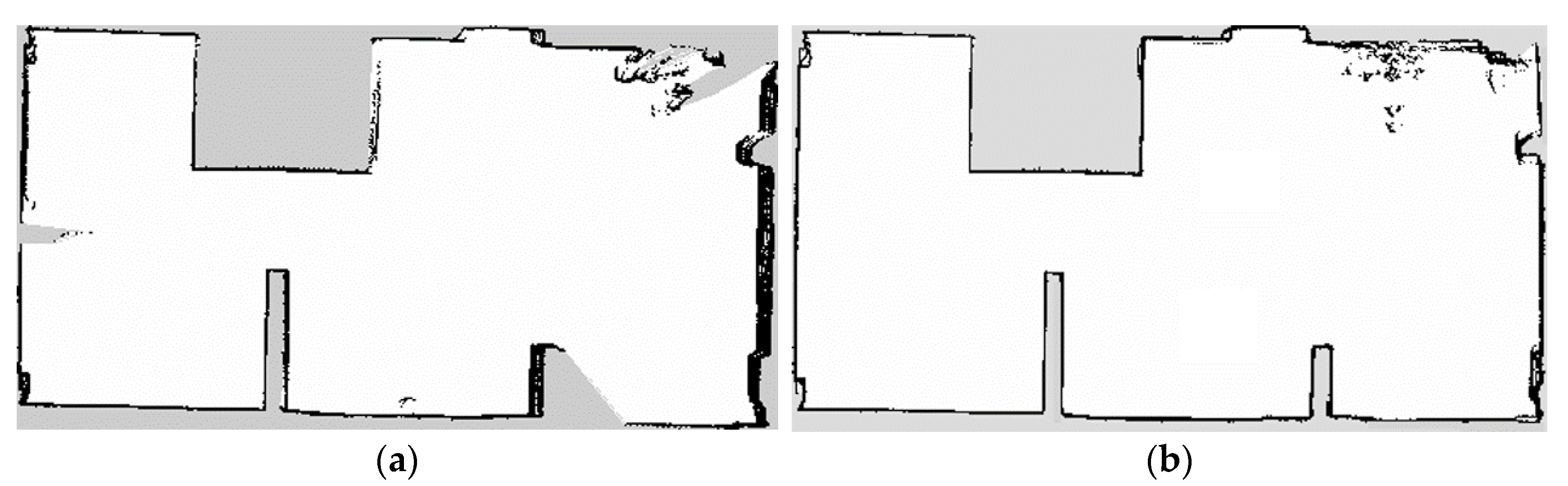
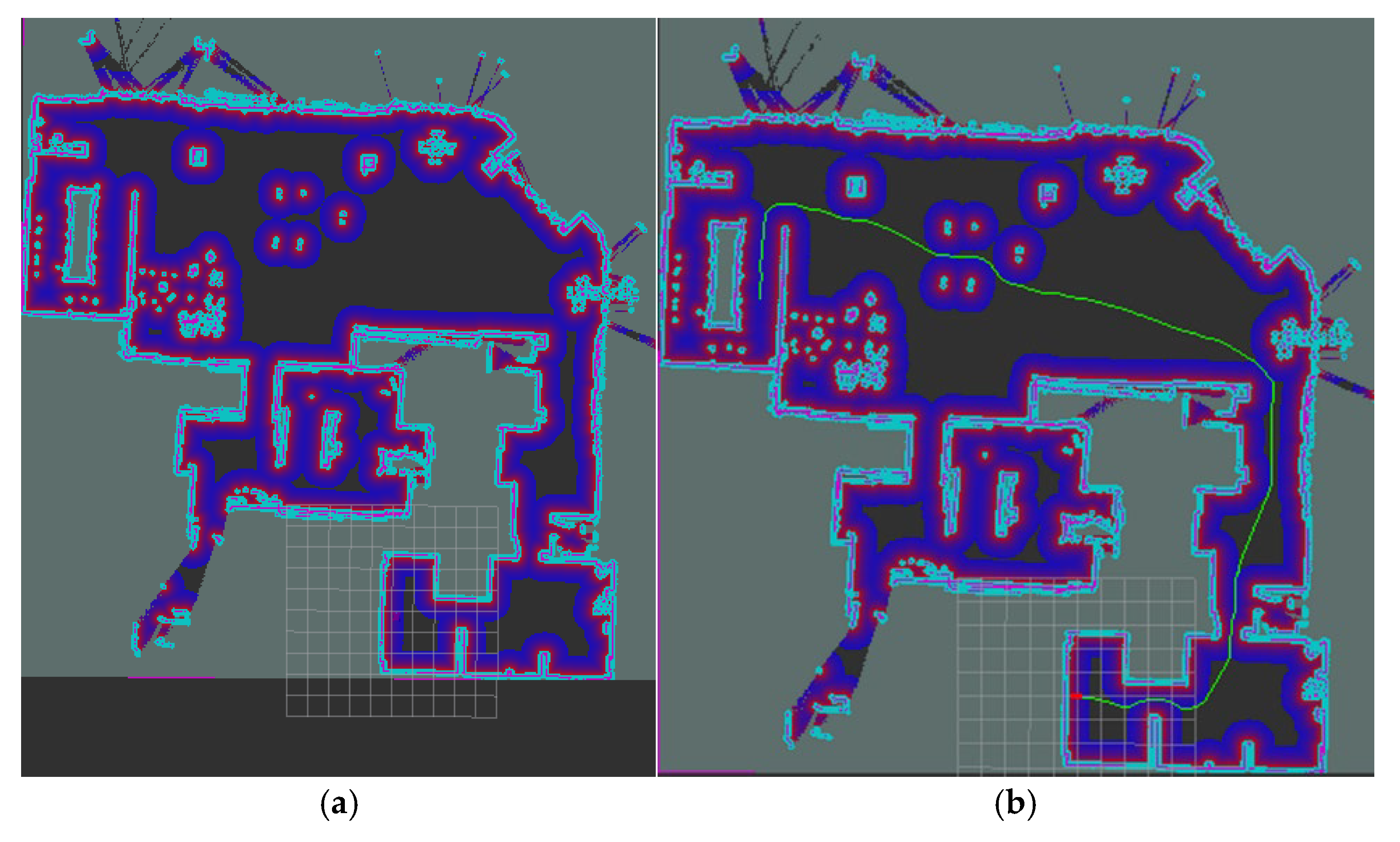
2.5.1. Indoor Mapping and Path Planning Test

The unmanned vehicle utilizes the Karto algorithm for large-scale mapping, which offers the advantage of low resource consumption [25]. The Karto algorithm requires inputs from a LIDAR and odometry data. However, the T265 visual odometry may produce inaccurate data in low-light conditions or when the device experiences shaking. To address this problem, this design utilizes the “robot_pose_ekf package” to fuse the T265 visual odometry data with IMU data from the Pixhawk 4 using an EKF, and outputs the fused data on the “odom” topic. This approach combines the strengths of both sensors to enhance the accuracy and robustness of the vehicle’s pose estimation.

Figure 5 illustrates indoor SLAM, where a two-dimensional grid map is constructed for the indoor environment. The vehicle is switched to manual control mode, and it is controlled to move at a speed of 1 m/s. During the movement, sensor data are collected and relevant features are extracted from the sensor data. These extracted features are then matched with previously observed features to establish correspondences at the same locations. Based on graph optimization techniques, the vehicle’s trajectory and environment map are estimated. Finally, loop closure is incorporated to correct accumulated errors in the map and trajectory.

After completing the mapping of the surrounding environment, the map is saved to the Raspberry Pi. The cost_map creates a costmap by loading a saved map file. Figure 6a shows the costmap created. The costmap is displayed in Rviz, and a 2D goal is set to define the target position for the unmanned vehicle. The adaptive Monte Carlo localization (AMCL) algorithm is used to estimate and update the position of the unmanned vehicle by performing probabilistic inference based on the vehicle’s motion and perception information. Once “move_base” receives the target position, it performs global path planning using the Dijkstra algorithm. After generating the global path, “move_base” employs a local path planning algorithm to generate a smooth local path near the robot’s current position. The local path planning algorithm usually takes into account the robot’s kinetic model and sensor information to ensure safe obstacle avoidance and movement along the global path. Once both the global and local paths are generated, “move_base” converts the local path into linear and angular velocity commands and sends them to the Pixhawk 4 via the “cmd_vel” topic. The ArduPilot firmware receives the linear and angular velocity data and controls the left and right motors to execute the path planning for the unmanned vehicle, as shown in Figure 6b. The green line in the figure represents the local path generated by the local path planning algorithm in “move_base”.

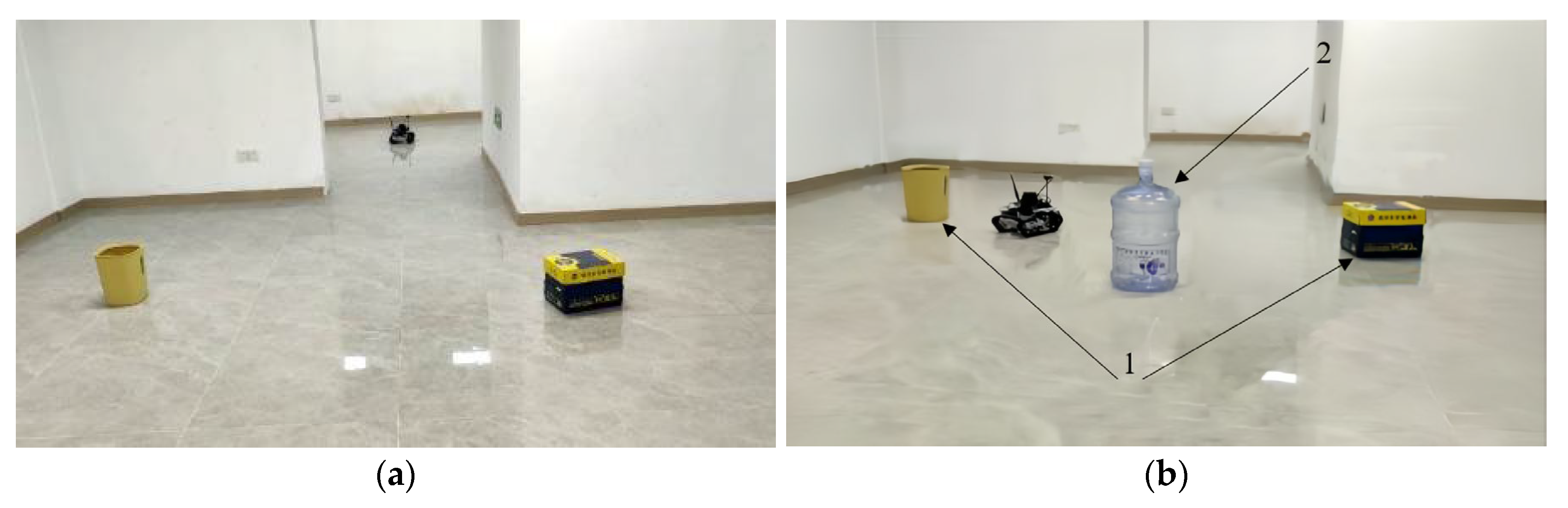
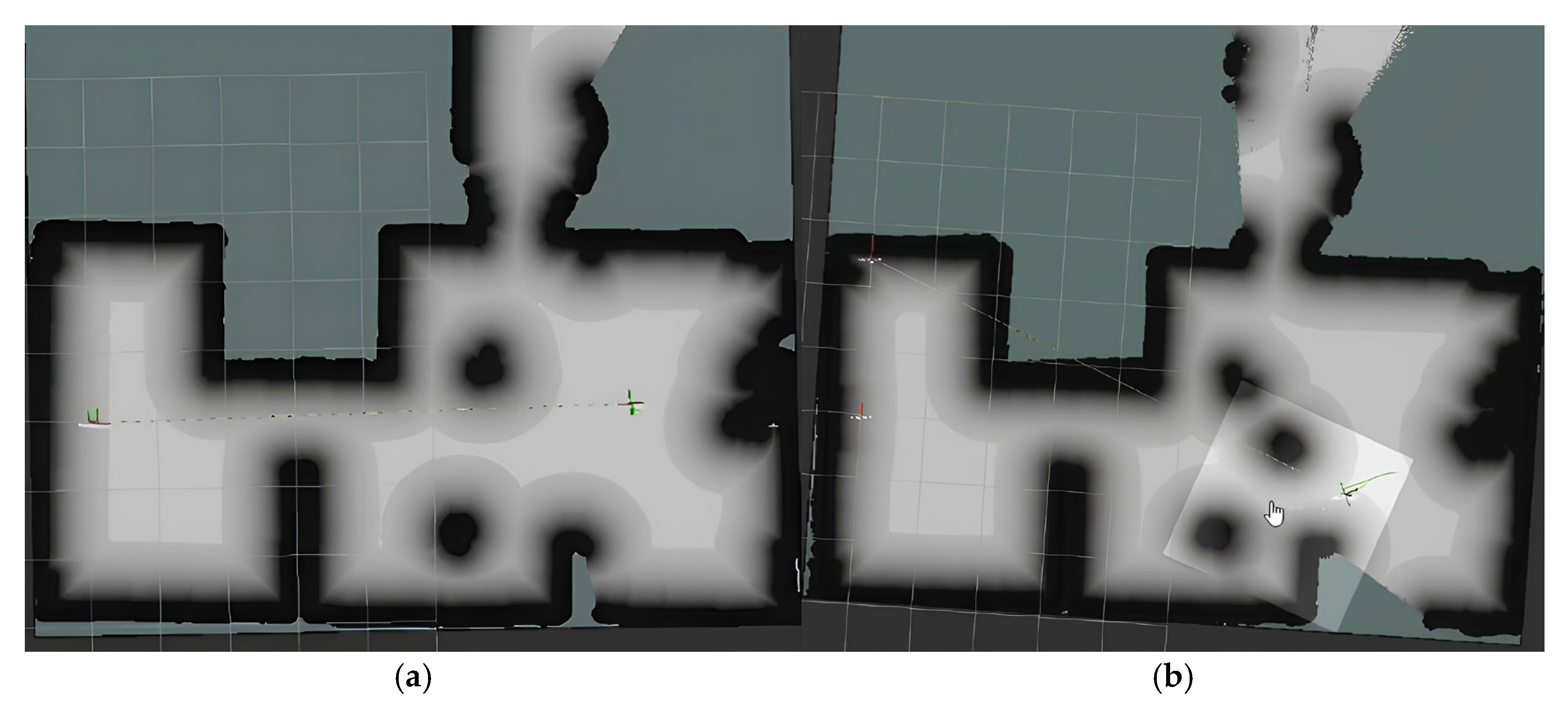
2.5.2. Indoor Obstacle Avoidance Test

To validate the system’s obstacle avoidance performance for temporary obstacles, this study conducted experiments on local path planning in an indoor environment. The purpose of local path planning is to enable the mobile robot to effectively avoid static and dynamic obstacles, ensuring safe and efficient movement along the predefined global path. The experimental process was as follows. First, the experimental environment was scanned, and a grid map was created. Then, two static obstacles were added to the original map, as shown in Figure 7a. Next, experiments were conducted on global path planning for the derivative drive vehicle. The system successfully controlled the vehicle to bypass the existing obstacles and reach the target position. Additionally, dynamic obstacles were introduced into the environment, as shown by the red box in Figure 7b, while the blue box represents static obstacles. The experimental results of global path planning and local path planning for the vehicle are shown in Figure 8a and Figure 8b, respectively. During the experiment, the vehicle’s target position was given in the form of a 2D goal in Rviz. The vehicle started moving based on the global path. During the movement, the vehicle continuously sensed the surrounding environment through a LIDAR and transmitted the perceived information to the local path planner. The local path planner, based on real-time perception of obstacle information, computed a feasible local path that avoids obstacles and sent it to the vehicle’s control system. This guided the vehicle to move along the locally planned path, avoiding temporary obstacles in the environment.

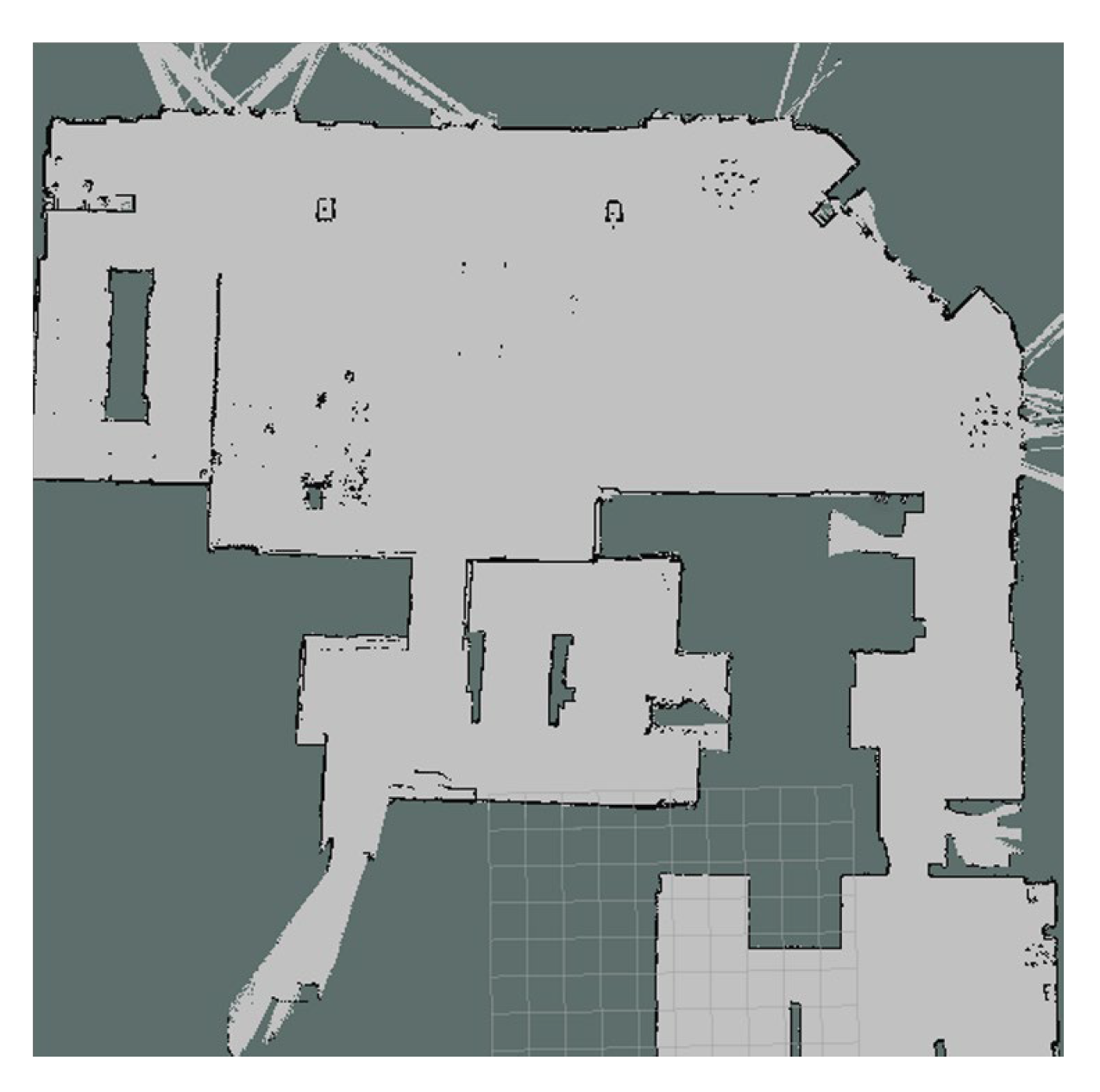
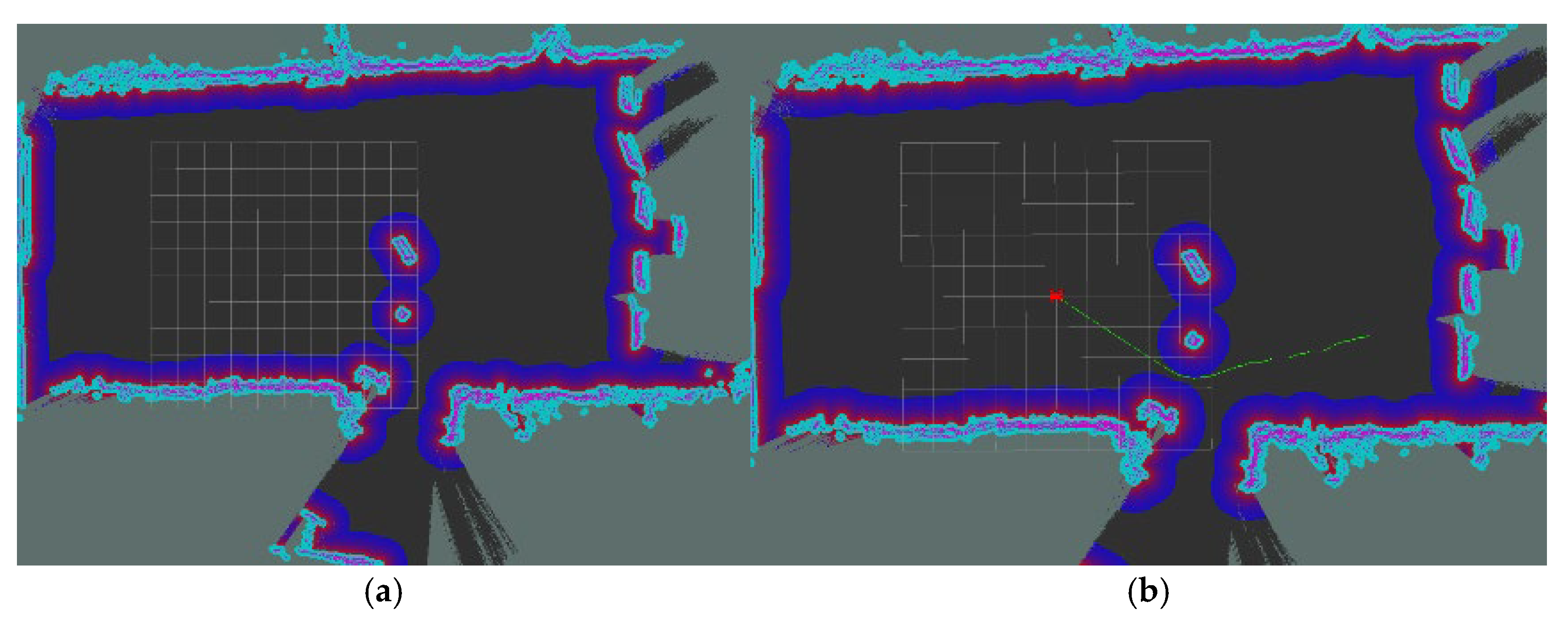
2.5.3. Outdoor Mapping and Path Planning Test

This study conducted mapping and obstacle avoidance experiments in an outdoor environment. The experimental site was located in Xiongdong Resettlement Area, Xiong County, as shown in Figure 9a. The model vehicle was placed in an appropriate position, and two cardboard boxes were used as obstacles. The LIDAR and visual odometry modules were initialized, and the model vehicle was manually controlled to obtain real-time information about the surrounding environment and perform SLAM. The mapping result is shown in Figure 9b. Due to the open nature of the environment, there was an incomplete boundary due to the open-ended outdoor setting. After completing the grid map creation for the outdoor environment, the grid map was loaded and a costmap was created, as shown in Figure 10a. The 2D goal method was used to specify the target position for the model vehicle in the costmap, similar to the indoor path planning approach. The system planned a path for the model vehicle and sent linear and angular velocities to the vehicle, as shown in Figure 10b. The green line in the figure represents the planned path. The model vehicle moved along the planned path and avoided obstacles based on the commanded linear and angular velocities.

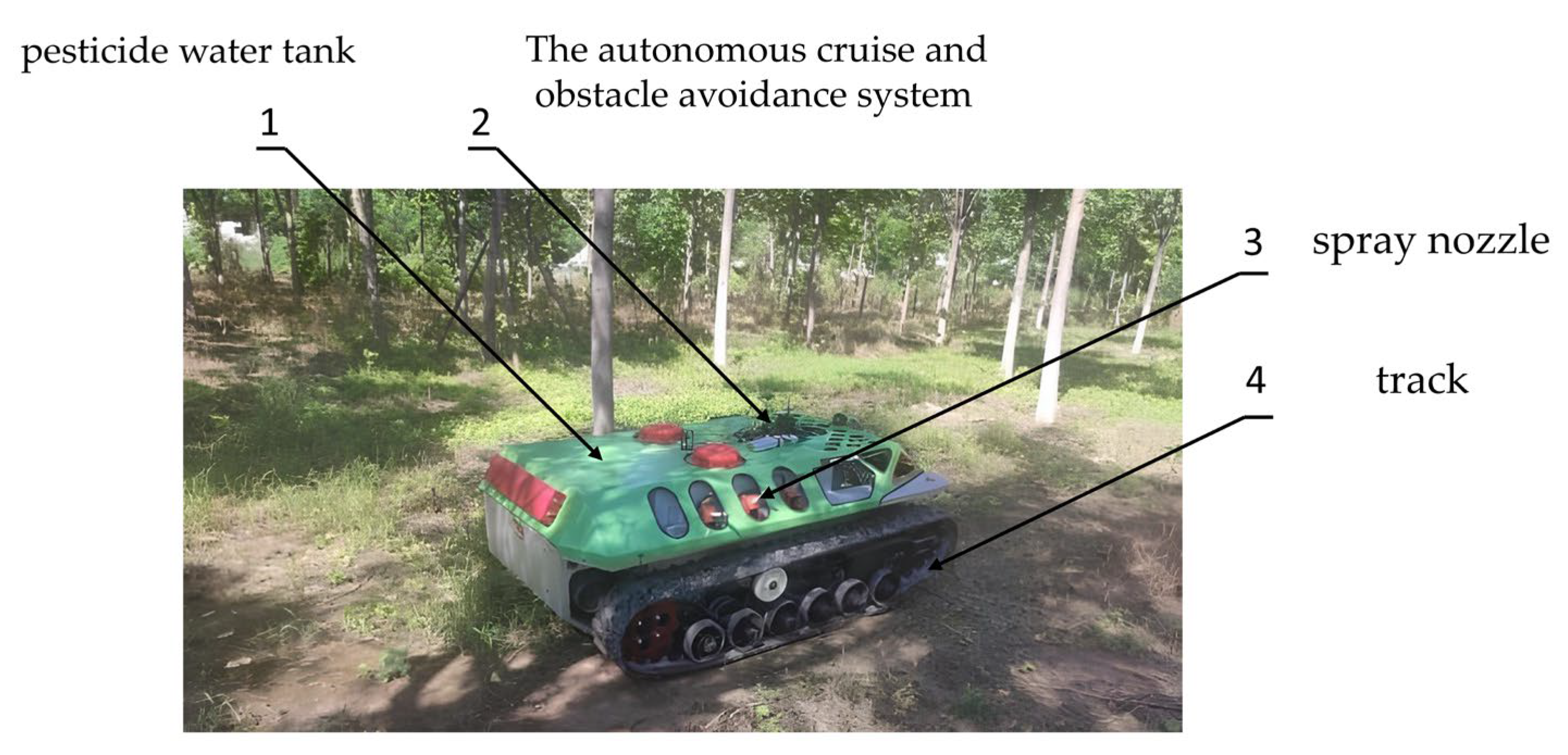
2.6. Modification of Unmanned Spraying Vehicles

After completing the indoor and outdoor navigation and sensor-fusion performance verification of the model vehicle, we applied it in practical application scenarios and systematically transformed the unmanned orchard spraying vehicle. Therefore, this section focuses on the hardware modification, control mode switching, and PID parameter optimization of the unmanned spraying vehicle and elaborates on how to transfer the core technologies verified by the model vehicle to an actual work vehicle to ensure the reliability and practicality of the algorithm in the real orchard environment.

The system modified the Tianyi 3WDZ–200D (Nonggu Feinong Plant Protection Technology Co., Ltd., Jinzhong, China) autonomous remote-controlled power sprayer, which is a remote-controlled tracked robot specifically designed for fruit tree plant protection. It is equipped with a 200 L pesticide water tank and incorporates fine-misting technology, capable of controlling the spray particle size within 100 μm and achieving a spraying range of 6–8 m, ensuring a more uniform coverage of the orchard with pesticides while saving water and reducing pesticide consumption by approximately 30%. The nozzles can be manually adjusted according to the operational environment (such as tree row spacing and height) to ensure targeted and comprehensive coverage, thereby enhancing the effectiveness of plant protection. It possesses remarkable adaptability and can operate flexibly in various terrains and orchard environments. Its tracked chassis and low bodywork enable it to rotate in place and maneuver between fruit trees.

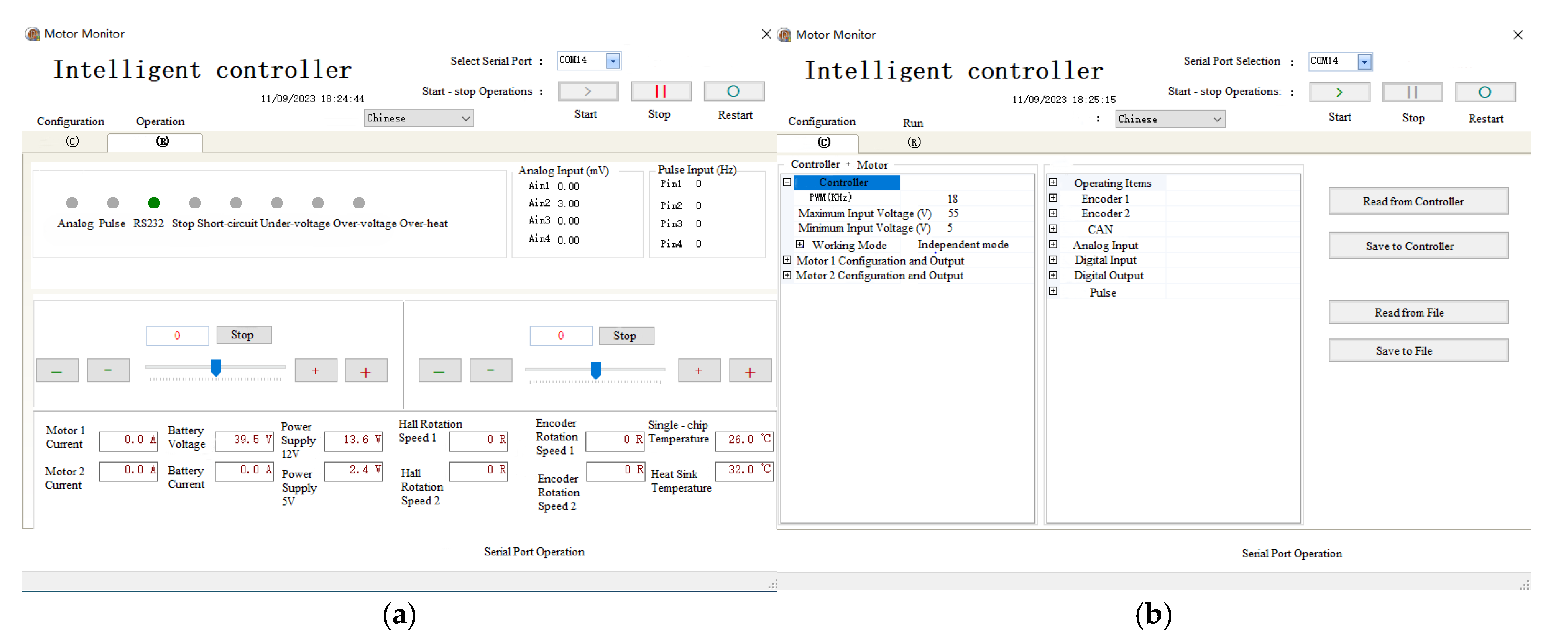
2.6.1. Servo Control Mode and ArduPilot Output Mode Changed

In this study, Motor Monitor version 1.0 (KEYA ELECTRON, Jinan, China) software was utilized to monitor the status and configure parameters of the servo controller. Figure 11a illustrates the main interface of the Motor Monitor software and the operational status of the servo controller. The servo controller offers four control modes: independent mode, hybrid mode 1, hybrid mode 2, and hybrid mode 3. Initially, the unmanned sprayer vehicle employed hybrid mode 1, where the steering and throttle were controlled through two signal lines, enabling remote control of the tracked vehicle’s movement using a remote controller. In this study, by adjusting the steering and throttle signals output by the ArduPilot, the remote controller was able to control the movement of the unmanned sprayer vehicle. However, the motion of the tracked vehicle could not be controlled through linear velocity and angular velocity signals. To address this problem, the control mode of the servo controller was changed to independent mode in this study, with the input being the signals from the two motors, as shown in Figure 11b.

In order to enable the unmanned sprayer vehicle to respond to angular velocity and linear velocity signals issued by an external computer, this study made adjustments to the output of Pixhawk 4. The original GroundSteering and Throttle signals were changed to ThrottleLeft and ThrottleRight signals, respectively. Additionally, the control mode of the servo controller was switched from hybrid mode 1 to independent mode. With these modifications, the unmanned sprayer vehicle can now be controlled both by a remote controller for the movement of the tracked vehicle and by an external computer for the movement control. This allows the vehicle to achieve the same control method and functionality as the model vehicle.

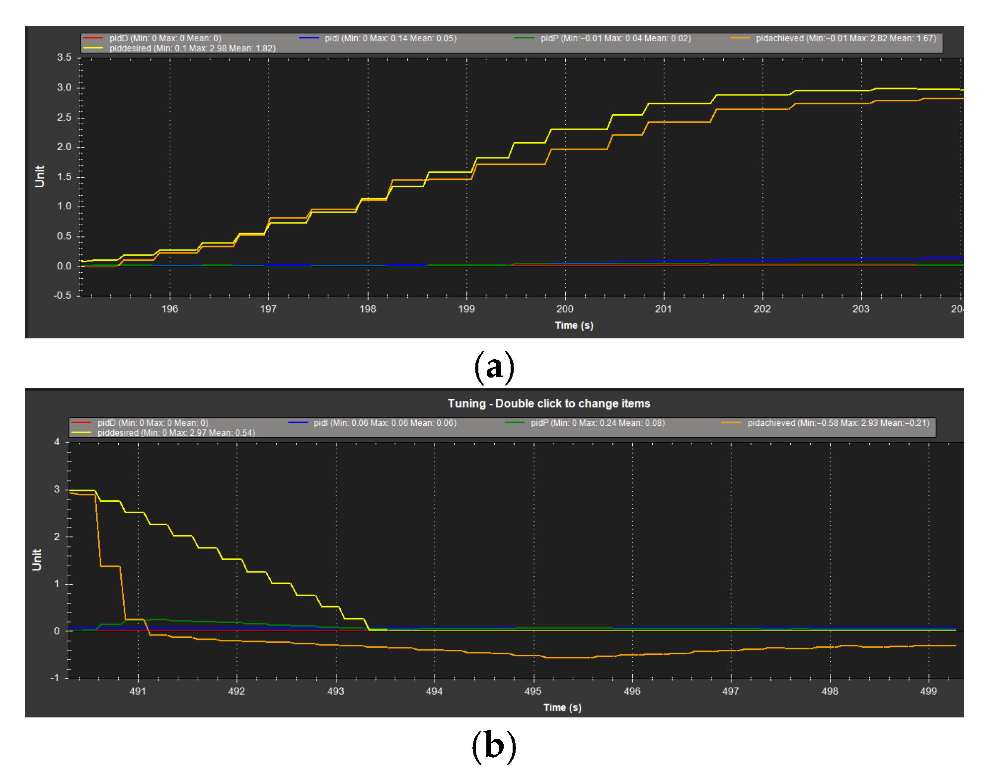
2.6.2. PID Control Parameter Adjustment

This study considered the differences in mass and inertia between the tracked chassis and the model vehicle chassis. It analyzed the potential oscillations or overshooting that may occur during turning or speed changes of the unmanned sprayer vehicle. To address this, a method based on a PID controller with derivative parameter adjustment was proposed. The derivative parameter adjusts the control input based on the rate of change in system state, enhancing the control system’s responsiveness to state variations. By optimizing the values of the derivative parameters, this study effectively suppressed the oscillations and overshooting of the unmanned sprayer vehicle, improving its stability and control accuracy during operation. Figure 12a illustrates the PID curve of the unmanned sprayer vehicle during acceleration, where the x-axis represents the system’s operating time and the y-axis represents the speed. The curve shows a stable and orderly upward trend during the acceleration phase. Figure 12b displays the PID curve of the unmanned sprayer vehicle during deceleration, with the x-axis representing the system’s operating time and the y-axis representing the speed. The curve demonstrates a smooth downward trend during the deceleration phase until the speed reaches zero. These results indicate that by adjusting the derivative parameters, smooth control during acceleration and deceleration of the unmanned sprayer vehicle was achieved, effectively enhancing overall stability and control accuracy during its operation.

2.7. Orchard Test of Unmanned Spraying Vehicle

The mapping and path planning experiments for the tracked vehicle were conducted in Sun Village Orchard, Xiongxian County, Hebei Province. Figure 13 shows an experimental scene of the unmanned vehicle in the orchard. In this orchard plot, the tree density is 10–15 trees per 100 square meters. In the areas with dense canopy cover measured by the GNSS signal strength logger, the GNSS occlusion rate ranged from 35% to 70%. In this experiment, the configuration parameters of the program were adjusted based on the length, width, and height of the tracked vehicle. This included parameters such as the vehicle size and the inflation radius of the costmap. The LIDAR sensor was installed at a height of 10 cm above the vehicle roof inclined forward at an angle of 10°, while the visual odometry camera was mounted at a height of 5 cm and aligned with the robot’s forward direction. During the experiments, light intensity values within the range of 200–1500 lux were recorded using a lux meter. Once the parameter settings were completed, the experiment first verified whether GPS could accurately locate the vehicle in dense fruit tree canopies. Then, the unmanned vehicle was manually controlled to perform SLAM in the orchard. After the mapping phase was completed, 2D goals were assigned to the unmanned vehicle, and path planning was carried out for reaching the target positions.

3. Results and Discussion

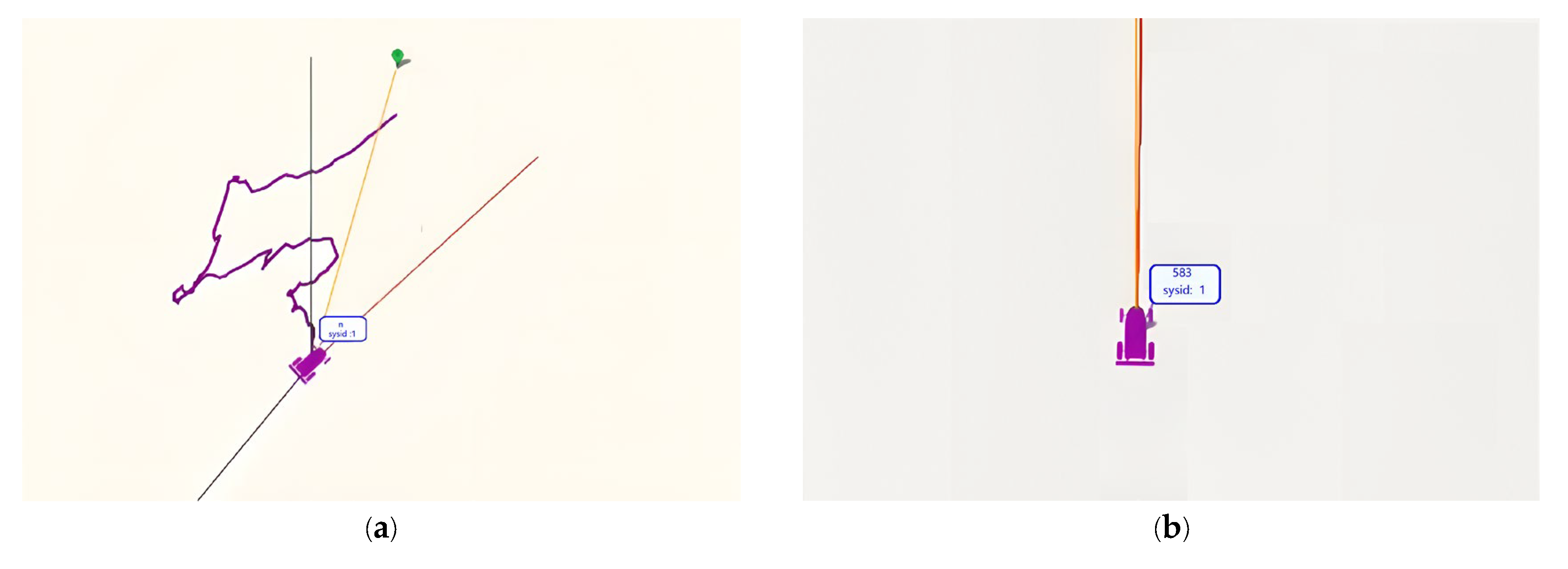
3.1. GPS Fusion Positioning

To validate the positioning performance of the modified tracked vehicle under fruit tree canopy occlusion, this study designed an EKF-based localization system that fuses data from the GPS and visual odometry. This system utilizes visual odometry data and coordinate transformation methods to estimate the position of the unmanned sprayer vehicle when GPS signal quality deteriorates due to canopy occlusion. Experimental results demonstrate that the system provides stable and accurate localization even in challenging environments with canopy occlusion. Figure 14a illustrates the significant position drift observed when using only GPS positioning for the unmanned sprayer vehicle under canopy occlusion. Red represents the current driving direction of the vehicle, green indicates north, yellow is the planned route, and purple is the actual driving route. Figure 14b shows a significant reduction in positioning error when GPS and visual odometry data are fused using the EKF approach.

3.2. Test Site Mapping and Path Planning Test

To create a 3D model of the surrounding orchard, the mapping software was launched and the control mode was switched to manual mode. The tracked vehicle was then controlled using a remote controller to drive at a speed of 2 m/s within the experimental area. The LIDAR installed on the tracked vehicle emitted and received laser beams, scanning the surrounding trees and calculating the distance and position of the trees based on the flight time of the laser beams. Simultaneously, the T265 visual odometry system recorded the vehicle’s motion trajectory and fused the data with the IMU data, enabling simultaneous localization and mapping of the surrounding environment. Figure 15 shows the results of the mapping.

After creating a 3D model of the orchard environment, a grid map was loaded to represent the structure of the orchard. In this study, a single target position was set using the 2D goal tool on the costmap, as shown in Figure 16a. A control strategy based on linear and angular velocities was then employed to guide the unmanned sprayer vehicle along the planned path, as depicted in Figure 16b.The green line in the figure is the travel path planned by the system for the unmanned sprayer vehicle, which can avoid obstacles such as trees and lead to the target position. During the path planning process, the system took into consideration the positions of obstacles such as trees, enabling the unmanned sprayer vehicle to effectively avoid them. By setting different target positions multiple times, the navigation performance of the unmanned sprayer vehicle was tested. In dense orchard environments, the average path planning time per iteration was approximately 260 milliseconds. The obstacle detection delay was ≤120 ms, achieved through optimized SLAM and sensor-fusion algorithms. The experimental results demonstrated that the unmanned sprayer vehicle could accurately reach the target position without collisions during its movement. This confirms the feasibility and effectiveness of the navigation control system for unmanned vehicles in real-world environments, providing strong support for intelligent navigation of the unmanned sprayer vehicle.

4. Discussion

(1)

Our proposed approach uses a combination of advanced sensors and algorithms. The SLAM and path planning functions enabled by Silan S2L LIDAR and T265 visual odometry help the vehicle move precisely in the orchard. This precision ensures that pesticides are sprayed only where necessary, reducing waste and improving utilization. The autonomous operation of the vehicle reduces human exposure to pesticides, protecting the health of workers. Moreover, the system’s ability to work continuously without human intervention throughout the spraying process represents a significant step towards improving automation levels.

(2)

The system may also face numerous challenges during actual deployment. The orchard terrain is complex, and environments such as slopes and soft soil can affect the vehicle’s stability and exacerbate mechanical wear. Strong light, dust, and other factors can interfere with the performance of sensors, affecting navigation and obstacle avoidance functions. In addition, long-term operation will lead to high energy consumption, and since power supply in orchards is limited, it is necessary to optimize power consumption or adopt sustainable energy sources. 4G communication is vulnerable to interference, which may affect real-time control, especially during critical operations such as obstacle avoidance. Therefore, the system needs to comprehensively optimize terrain adaptability, environmental tolerance, energy management, and communication stability to ensure reliable operation.

(3)

The development of the orchard spraying robot system has two primary future directions: integrating with smart agriculture systems and optimizing sensor-fusion algorithms. For the first direction, while connecting to smart agriculture networks could enable dynamic adjustments of spraying strategies based on real-time weather, soil nutrient, and pest data to enhance plant protection efficiency, challenges such as interoperability between heterogeneous platforms, data standardization, and reliable field communication (e.g., signal attenuation in dense canopies) must be addressed. The second direction involves exploring machine learning-based advanced sensor-fusion techniques to improve positioning accuracy and adaptability to complex environments, though key hurdles include developing lightweight models compatible with low-power hardware and ensuring model generalization across diverse orchard scenarios.

5. Conclusions

This study presents an autonomous cruising and obstacle avoidance system for unmanned sprayer vehicles based on ArduPilot firmware and ROS. Aiming at the challenge of GNSS signal occlusion in unstructured outdoor orchard environments, a multi-sensor positioning and mapping method fusing GPS, LIDAR, IMU, and visual odometry is designed. An EKF is employed to construct a loosely coupled fusion framework, dynamically integrating GPS positioning information, LIDAR environmental perception data, IMU high-frequency motion parameters, and visual odometry data. This approach effectively addresses the limitations of single sensors in signal occlusion, dynamic lighting changes, and complex terrains, significantly enhancing the positioning accuracy and attitude estimation robustness of tracked vehicles in complex orchard scenarios. However, the system exhibits specific limitations: discrepancies between data formats and sampling frequencies among sensors introduce time synchronization errors and coordinate mismatches during fusion, compromising positioning consistency. Additionally, during turns, visual odometry is prone to feature matching failures due to motion blur, exacerbating heading angle error accumulation. Also, changes in LIDAR scan angles cause point cloud sparsity, further increasing the risk of dynamic obstacle detection failure. Future research will focus on improving sensor-fusion strategies, including implementing advanced time-alignment techniques and adaptive fusion frameworks to dynamically adjust sensor weightings, optimizing visual odometry feature extraction algorithms to mitigate motion blur and reduce heading angle errors, and enhancing environmental perception through multi-angle LIDAR deployment to increase point cloud density for more accurate obstacle detection. These improvements will enhance the system’s positioning and navigation accuracy, enabling more reliable autonomous navigation in smart orchard management.

References

1. Hu, Y.; Yang, H.; Hou, B.; Xi, Z.; Yang, Z. Influence of Spray Control Parameters on the Performance of an Air-Blast Sprayer. Agriculture 2022, 12, 1260. [Google Scholar] [CrossRef]
2. Ranta, O.; Marian, O.; Muntean, M.V.; Molnar, A.; Ghețe, A.B.; Crișan, V.; Stănilă, S.; Rittner, T. Quality Analysis of Some Spray Parameters When Performing Treatments in Vineyards in Order to Reduce Environment Pollution. Sustainability 2021, 13, 7780. [Google Scholar] [CrossRef]
3. Zhao, Y.; Xiao, H.R.; Mei, S.; Song, Z.Y.; Ding, W.Q.; Jin, Y.; Han, Y.; Xia, X.F.; Yang, G. Current Status and Development Strategies of Orchard Mechanization Production in China. J. China Agric. Univ. 2017, 22, 116–127. (In Chinese) [Google Scholar]
4. Zheng, Y.J.; Chen, B.T.; Lyu, H.T.; Kang, F.; Jiang, S.J. Research progress of orchard plant protection mechanization technology and equipment in China. Trans. Chin. Soc. Agric. Eng. 2020, 36, 110–124. (In Chinese) [Google Scholar]
5. Du, J.; Liu, X.; Meng, C. Road Intersection Extraction Based on Low-Frequency Vehicle Trajectory Data. Sustainability 2023, 15, 14299. [Google Scholar] [CrossRef]
6. Etezadi, H.; Eshkabilov, S. A Comprehensive Overview of Control Algorithms, Sensors, Actuators, and Communication Tools of Autonomous All-Terrain Vehicles in Agriculture. Agriculture 2024, 14, 163. [Google Scholar] [CrossRef]
7. Huang, Y.; Fu, J.; Xu, S.; Han, T.; Liu, Y. Research on Integrated Navigation System of Agricultural Machinery Based on RTK-BDS/INS. Agriculture 2022, 12, 1169. [Google Scholar] [CrossRef]
8. Jagelčák, J.; Kuba, O.; Kubáňová, J.; Kostrzewski, M.; Nader, M. Dynamic Position Accuracy of Low-Cost Global Navigation Satellite System Sensors Applied in Road Transport for Precision and Measurement Reliability. Sustainability 2024, 16, 5556. [Google Scholar] [CrossRef]
9. Han, J.H.; Park, C.H.; Park, Y.J.; Kwon, J.H. Preliminary results of the development of a single−frequency GNSS RTK−based autonomous driving system for a speed sprayer. J. Sens. 2019, 2019, 4687819. [Google Scholar] [CrossRef]
10. Xiong, B.; Zhang, J.X.; Qu, F.; Fan, Z.Q.; Wang, D.S.; Li, W. Navigation Control System for Orchard Spraying Machine Based on Beidou Navigation Satellite System. Trans. Chin. Soc. Agric. Mach. 2017, 48, 45–50. (In Chinese) [Google Scholar]
11. Shang, Y.; Wang, H.; Qin, W.; Wang, Q.; Liu, H.; Yin, Y.; Song, Z.; Meng, Z. Design and Test of Obstacle Detection and Harvester Pre-Collision System Based on 2D Lidar. Agronomy 2023, 13, 388. [Google Scholar] [CrossRef]
12. Hu, C. Research on Positioning and Map Construction of Orchard Operating Robots. Master’s Thesis, Nanjing Agricultural University, Nanjing, China, 2015. (In Chinese). [Google Scholar]
13. Hu, L.; Wang, Z.M.; Wang, P.; He, J.; Jiao, J.K.; Wang, C.Y.; Li, M.J. Agricultural robot positioning system based on laser sensing. Trans. Chin. Soc. Agric. Eng. 2023, 39, 1–7. (In Chinese) [Google Scholar]
14. Shi, X.; Wang, S.; Zhang, B.; Ding, X.; Qi, P.; Qu, H.; Li, N.; Wu, J.; Yang, H. Advances in Object Detection and Localization Techniques for Fruit Harvesting Robots. Agronomy 2025, 15, 145. [Google Scholar] [CrossRef]
15. Adrien, D.P.; Emile, L.F.; Viviane, C.; Thierry, S.; Stavros, V. Tree detection with low−cost three−dimensional sensors for autonomous navigation in orchards. IEEE Robot. Autom. Lett. 2018, 3, 3876–3883. [Google Scholar]
16. Fei, K.; Mai, C.; Jiang, R.; Zeng, Y.; Ma, Z.; Cai, J.; Li, J. Research on a Low-Cost High-Precision Positioning System for Orchard Mowers. Agriculture 2024, 14, 813. [Google Scholar] [CrossRef]
17. Yin, X.; Wang, Y.X.; Chen, Y.L.; Jin, C.Q.; Du, J. Development of autonomous navigation controller for agricultural vehicles. Int. J. Agric. Biol. Eng. 2020, 13, 70–76. [Google Scholar] [CrossRef]
18. Marucci, A.; Colantoni, A.; Zambon, I.; Egidi, G. Precision Farming in Hilly Areas: The Use of Network RTK in GNSS Technology. Agriculture 2017, 7, 60. [Google Scholar] [CrossRef]
19. Iberraken, D.; Gaurier, F.; Roux, J.-C.; Chaballier, C.; Lenain, R. Autonomous Vineyard Tracking Using a Four-Wheel-Steering Mobile Robot and a 2D LiDAR. AgriEngineering 2022, 4, 826–846. [Google Scholar] [CrossRef]
20. Fujinaga, T. Autonomous navigation method for agricultural robots in high-bed cultivation environments. Comput. Electron. Agric. 2025, 231, 110001. [Google Scholar] [CrossRef]
21. Ospina, R.; Itakura, K. Obstacle Detection and Avoidance System Based on Layered Costmaps for Robot Tractors. Smart Agric. Technol. 2025, 11, 100973. [Google Scholar] [CrossRef]
22. Jiang, S.; Qi, P.; Han, L.; Liu, L.; Li, Y.; Huang, Z.; Liu, Y.; He, X. Navigation System for Orchard Spraying Robot Based on 3D LiDAR SLAM with NDT_ICP Point Cloud Registration. Comput. Electron. Agric. 2024, 220, 108870. [Google Scholar] [CrossRef]
23. Liu, H.; Zeng, X.; Shen, Y.; Xu, J.; Khan, Z. A Single-Stage Navigation Path Extraction Network for Agricultural Robots in Orchards. Comput. Electron. Agric. 2025, 229, 109687. [Google Scholar] [CrossRef]
24. Zhang, Y.; Sun, H.; Zhang, F.; Zhang, B.; Tao, S.; Li, H.; Qi, K.; Zhang, S.; Ninomiya, S.; Mu, Y. Real-Time Localization and Colorful Three-Dimensional Mapping of Orchards Based on Multi-Sensor Fusion Using Extended Kalman Filter. Agronomy 2023, 13, 2158. [Google Scholar] [CrossRef]
25. Chang, C.-L.; Chen, H.-W.; Ke, J.-Y. Robust Guidance and Selective Spraying Based on Deep Learning for an Advanced Four-Wheeled Farming Robot. Agriculture 2024, 14, 57. [Google Scholar] [CrossRef]
Figure 1. Block diagram of system hardware.
Agronomy 15 01373 g001
Figure 2. Architecture diagram of system software.
Agronomy 15 01373 g002
Figure 3. Model vehicle test platform.
Agronomy 15 01373 g003
Figure 4. Comparison of fused data construction using extended Kalman filtering: (a) Using T265 visual odometry data separately for mapping; (b) using extended Kalman filter to fuse data for mapping.
Agronomy 15 01373 g004
Figure 5. SLAM of indoor environment.
Agronomy 15 01373 g005
Figure 6. Costmap and path planning for indoor environment: (a) costmap of indoor environment; (b) path planning for indoor environment.
Agronomy 15 01373 g006
Figure 7. Placement of obstacles in the experimental environment: (a) existing obstacles; (b) temporary obstacles. 1. Fixed obstacles; 2. Temporary obstacle.
Agronomy 15 01373 g007
Figure 8. Global and local path planning experiments: (a) global path planning; (b) local path planning.
Agronomy 15 01373 g008
Figure 9. Model car outdoor testing and SLAM of outdoor environment: (a) model car outdoor experiment; (b) SLAM of outdoor environments.
Agronomy 15 01373 g009
Figure 10. Costmap and path planning for outdoor environment: (a) costmap of outdoor environment; (b) path planning for outdoor environments.
Agronomy 15 01373 g010
Figure 11. Motor Monitor server control software: (a) working status of the server; (b) server changes working mode.
Agronomy 15 01373 g011
Figure 12. PID parameters of unmanned spraying vehicle: (a) PID value during acceleration; (b) PID value during deceleration.
Agronomy 15 01373 g012
Figure 13. Orchard test of an unmanned spraying vehicle.
Agronomy 15 01373 g013
Figure 14. Comparison of GPS data fusion before and after: (a) GPS positioning under canopy occlusion; (b) GPS and visual odometer data fusion positioning.
Agronomy 15 01373 g014
Figure 15. SLAM of surrounding forests.
Agronomy 15 01373 g015
Figure 16. Costmap and path planning of forest environment: (a) costmap of forest environment; (b) path planning for forest environment.
Agronomy 15 01373 g016