Article

Topographic Position Index Predicts Within-Field Yield Variation in a Dryland Cereal Production System

by
Jacob A. Macdonald
1,2,
David M. Barnard
1,
Kyle R. Mankin
1,*,
Grace L. Miner
3,
Robert H. Erskine
1,
David J. Poss
3,
Sushant Mehan
4,
Adam L. Mahood
1 and
Maysoon M. Mikha
1
1
Water Management & Systems Research Unit, USDA-ARS, 2150 Centre Ave., Fort Collins, CO 80526, USA
2
Colorado State University Extension, 1311 S College Ave., Fort Collins, CO 80523, USA
3
Soil Management & Sugar Beet Research Unit, USDA-ARS, 2150 Centre Ave., Fort Collins, CO 80526, USA
4
Agricultural & Biosystems Engineering Department, South Dakota State University, 1030 N Campus Dr., Brookings, SD 57007, USA
*
Author to whom correspondence should be addressed.
Agronomy 2025, 15(6), 1304; https://doi.org/10.3390/agronomy15061304
Submission received: 17 March 2025 / Revised: 27 April 2025 / Accepted: 29 April 2025 / Published: 27 May 2025

Abstract

:
Agricultural systems exhibit a large degree of within-field yield variability. We require a better understanding of the drivers of this variability in order to optimally manage croplands. We investigated drivers of sub-field spatial variability in yield for three crops (hard red winter wheat, Triticum aestivum L. variety Langin; corn, Zea mays L.; and proso millet, Panicum milaceum L.) usings a multi-year dataset from a dryland research farm in northeastern Colorado, USA. The dataset spanned 18 2.6–4.3 ha management units, over 4 years, and included high-resolution topographic data, densely sampled soil properties, and on-site weather data. We modeled yield for each crop separately using random forest regression and evaluated model performance using spatially blocked cross-validation. The topographic position index (TPI) and increasing percent sand had a strong negative effect on yield, while the nitrogen application rate (N) and total soil carbon had strong positive effects on yield in both the wheat and millet models. Remarkably, TPI had almost as large of an effect size as N, and outperformed other more commonly used topographic predictors of yield such as the topographic wetness index (TWI), elevation, and slope. Despite the size and quality of our dataset, cross-validation results revealed that our models account for approximately one-quarter of the total yield variance, highlighting the need for continued research into drivers of spatial variability within fields.

1. Introduction

Agricultural systems often exhibit a large amount of within-field variability in crop yields largely attributable to variations in soil, topography, management, and weather (e.g., [1,2,3,4]). However, the processes and interactions driving this variability are not fully understood, particularly in dryland agricultural systems, limiting our ability to optimally manage croplands. Semi-arid dryland regions are marked by high temporal and spatial weather variability, high evapotranspiration, and recurring periods of severe drought [5]. Tools to assess and optimally manage yield variability and production risk are critically imperative for dryland producers operating in tight margins. Precision agriculture, broadly defined as an applied suite of principles and technologies to assess and manage spatial and temporal variability in agricultural yields, offers strategies to make management decisions in a spatially explicit manner to optimize yields, environmental benefits, and economic outcomes [6,7]. These methods can mitigate the drawbacks that low-yielding or highly temporally variable areas of fields cause (e.g., wasted inputs, economic losses) and improve environmental and economic outcomes [8,9,10].
One such precision management strategy is the adoption of distinct management zones within a field. Crop yields are influenced by multiple drivers of heterogeneity, including natural variation in soil and topography, weather, and managed inputs. Disentangling soil–yield relationships from weather and management requires multiple years of geospatially explicit yield-monitoring data [10,11,12]. With these data, management zones can be delineated by various methods (cf. [8]), with common approaches of aggregation and categorization of yield data for each field location according to average prior yields (e.g., high, medium, low) or according to both yield and yield stability metrics (e.g., high yield–high stability, high yield–low stability, etc.). Sometimes topographic data, soil characteristics, or remotely sensed spectral data are also included in the delineation process to create management zones of presumed homogeneity with regard to yield potential [8,13]. Different management practices can then be applied to each zone, tailored to the specific needs of the crops within that zone. However, there are challenges and theoretical limitations of this approach. First, spatial patterns in yield are often inconsistent from year to year [11], bringing additional complexity to static zone management. Indeed, both historic and recent work have highlighted instability in spatial patterns of yield potential [3,10,14]. Second, yield is the net integration of many processes. Different areas of a field might fall into the same yield category for different reasons, and may therefore require different management practices to optimize performance (e.g., [3]). Finally, we need a better understanding of the individual and interactive processes driving yield variability in order to accurately predict and optimally manage future crop performance, as past crop performance may not be an indicator of future performance in light of changing weather patterns [15,16].
Many studies have found associations between elevation and yield [2,16,17,18], but the strength and direction of the relationship can vary [4,19,20], and there is a lack of consistent mechanistic explanations for this relationship. Moreover, elevation as a modeling variable is only relevant to a specific field or farm, thus including it as a predictor in broader models will limit the ability to extrapolate findings elsewhere. At the within-field scale, elevation can be correlated with numerous factors that have the potential to influence crop growth, including soil texture, soil chemistry, and nutrient availability [21,22]. Elevation also affects insolation, as well as patterns of surface runoff and below-ground water movement [23,24]. Therefore, disentangling which correlates of elevation are the most important predictors of crop performance is essential for developing an understanding of the processes involved.
Production in semi-arid dryland systems faces multiple constraints, including soils characterized by low soil organic matter and poor fertility, low regional precipitation coupled with high atmospheric demand, and high intra- and interannual variability of water and temperature stress [25,26]. Large interannual differences in weather result in highly variable dryland crop yields [27,28,29]. Spatial variability within-field due to landscape effects such as soils and topography can be difficult to disentangle from these large interannual yield differences. Efforts to understand drivers of spatial variability are further complicated due to the fact that landscape factors’ relationships with yield can change under different weather conditions [2,3,18,30,31]. Thus, we can expect interannual variability to affect the overall magnitude of yield, as well as the spatial patterns and drivers of yield. Large multi-year datasets are required to have the statistical power to determine the effects of weather, landscape effects, and their interactions on yield, but such large datasets are rare.
Predictor variables in the landscape tend to be correlated with each other, making it hard to design experiments stratified by just one predictor of interest. This collinearity, coupled with the interannual variability in yield and yield–predictor relationships, makes conducting controlled, well-replicated experiments costly and time-consuming. Gathering observational data, on the other hand, has become relatively easy due to the adoption of yield monitors coupled with GPS units. While experimentation is necessary to determine the mechanistic drivers of yield definitively, observational studies give us the opportunity to begin inferring relationships and generating hypotheses, which will aid in designing future experiments. While yield and elevation data are readily available, soil property data require more effort to collect. Most studies in dryland systems to date have been lacking in densely sampled soil data.
Traditional statistical methods, such as generalized linear models, can be challenging to apply to observational crop yield datasets due to non-linear or non-monotonic yield–predictor variable relationships, collinearity among predictors, and the sheer number of potentially important predictor and interaction terms. Many of these challenges can be overcome with the use of machine learning models such as random forest regression [32,33]. Random forest has been shown to be among the best machine learning techniques for predicting crop yields [1,34]. However, care must be taken when drawing inferences and evaluating the performance of machine learning models. When data points are not independent, the simple cross-validation of model performance on randomly sampled data points leads to overestimation of model accuracy and overfitting [35]. When dependence structures are present in the data, a better method of model evaluation is to cross-validate using subsets of the data that are blocked with respect to the dependence structure present (e.g., temporarily blocked or spatially blocked) [35]. Studies of fine scale spatial variability are almost certain to have a strong dependence structure due to spatial autocorrelation, which has been demonstrated in yield values in a variety of systems [10,20,36]. However, many studies evaluating drivers of fine-scale spatial variability of yield have not utilized independent data points when evaluating model performance (e.g., [2,4,14,18,34,37,38]), suggesting that past reports on the predictive capacity of statistical or machine learning yield models may be substantially overestimated.
Here, we capitalize on a large dataset from a dryland system in a semi-arid region of northeastern Colorado, which spans 4 years, eighteen 2.6–4.3 ha management units, and three crop types. We use random forest regression to model yield and gain insight into within-field spatial patterns of yield variability. This dataset contains uniquely high-resolution sampling of soil properties, N application, and topography in a dryland system, allowing us to address the following research questions with greater confidence:
  • What landscape characteristics (i.e., soil characteristics and topographic influences) are most important in driving spatial variability of crop yield at the within-field scale over multiple years with variable precipitation?
  • Given the considerable resolution of our dataset, what inferences can be made about data needs in future studies and applications to improve our ability to model and understand past crop yields, apply models in an operational forecasting capacity, and direct future data collection efforts?
Improving our understanding of the drivers of yield variability will bring us closer to developing management strategies informed by the mechanistic processes that drive yield. Such strategies will be more robust to weather variability and non-stationarity compared to management strategies that delineate zones of expected yield based on historical outcomes. Additionally, careful consideration of model performance, or lack thereof, will help generate hypotheses about sources of unexplained variance, guiding future research efforts.

2. Materials and Methods
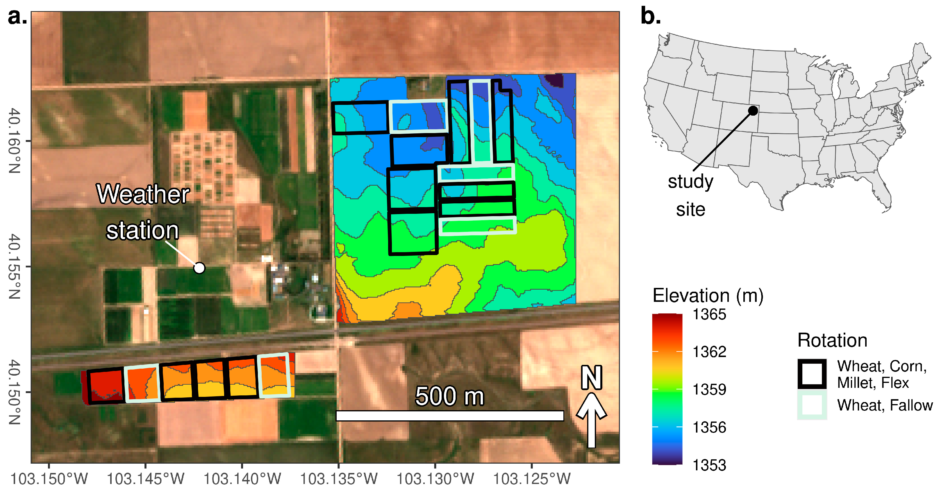
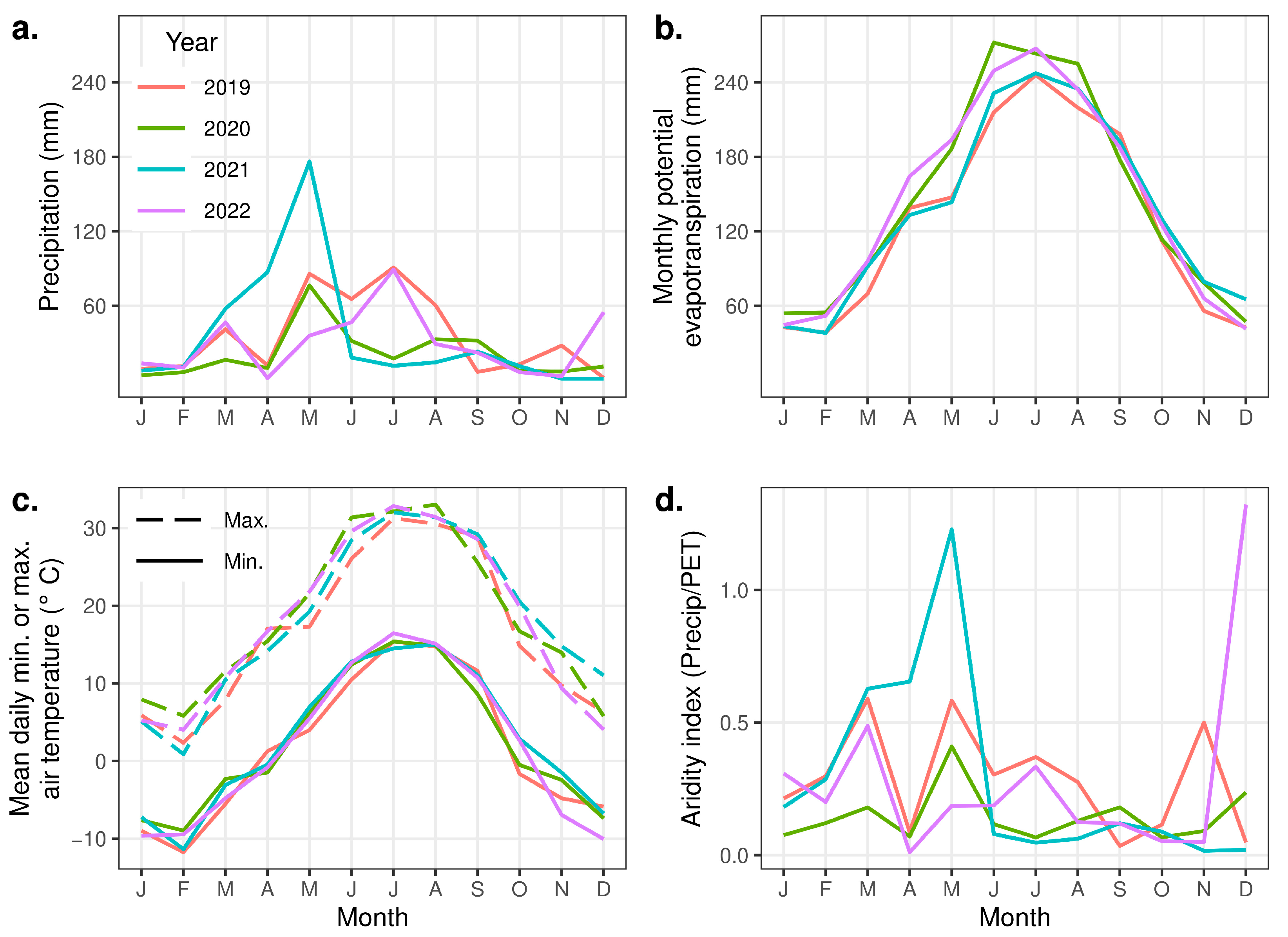
2.1. Study Site

The management units in this study were located at the USDA-ARS Central Great Plains Research Station (40.155° N, 103.135° W) located 6.4 km east of Akron, Colorado (Figure 1b). The management units occur in two distinct clusters separated by approximately 300 m (Figure 1a). Across all management units, elevation ranged from 1353 to 1365 m, and slopes were below 4%. Soils included Ascalon sandy loam (fine-loamy, mixed, superactive, mesic Aridic Argiustolls), Platner loam (fine, smectitic, mesic Aridic Paleustolls), Rago silt loam (fine, smectitic, mesic Pachic Argiustolls), and Weld silt loam (fine, smectitic, mesic Aridic Argiustolls) [39,40].
Meteorologic data were collected by an onsite weather station (Figure 1a). This site is characterized by a semi-arid climate (Figure 2a) in which evaporative demand typically greatly exceeds rainfall during the growing season (Figure 2d), with cold winters and warm summers (Figure 2c). During the 4-year study period, early summer precipitation (1 May through 15 June), a critical time period for winter wheat, ranged from 83 to 177 mm. The full summer precipitation (May through August), which roughly coincides with the growing season for corn and millet, ranged from 159 to 303 mm.

2.2. Cropping Practices
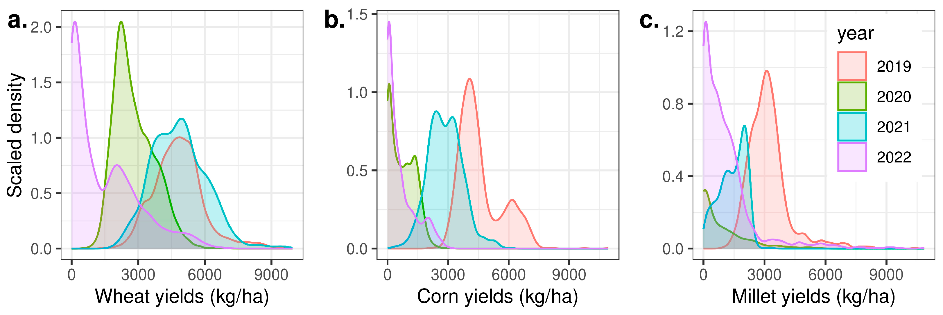
This study included two crop rotations: wheat–fallow (WF) and wheat–corn–millet–flex (WCMFx) with each crop phase (2 WF management units, 4 WCMFx management units) present each year with 3 replications (18 management units total). Management units ranged from 2.6 to 4.3 ha. WF was a 2-year rotation with hard red winter wheat, Triticum aestivum L., variety Langin, followed by 14-month chemical fallow with reduced tillage. Tillage included sweep tillage with horizontal v-blades (8–10 cm depth) in August, followed by disk-tillage immediately before planting if needed to control weeds or if the wheat stubble was too thick to plant into. Herbicides (glyphosate [Nufarm Americas Inc., Alsip, IL, USA], 2,4-D herbicide [Alligare, Opelika, AL, USA], dicamba [3,6-dichloro-2-methoxybenzoic acid; Alligare, Opelika, AL, USA], paraquat [1,10-dimethyl-4,40-bipyridinium dichloride; Solera, Yuma, AZ, USA], Thifensulfuron-methyl [FCM, Philadelphia, PA, USA], Tribenuron-methyl [FCM, Philadelphia, PA, USA], or Metsulfuron-methyl [FCM, Philadelphia, PA, USA]) were applied, as needed during crop and non-crop periods. WCMFx was a 4-year rotation with winter wheat, corn (Zea mays L.), proso millet (Panicum milaceum L.), and a flexible decision made at the planting of either fallow (12.5 month chemical fallow with no tillage) or foxtail millet (Setaria italica L. Beauv.) as a forage crop based on an analysis of linear yield vs. the water use production function, measured available soil water, and expected precipitation [41]. Planting dates each year were late September for wheat, mid to late May for corn, and early June for millet. Crop row spacings were 30 cm for wheat in the WF rotation, or 19 cm for wheat, 76 cm for corn, and 19 cm for millet in the WCMFx rotation. Additional site and experimental details are presented in Mikha et al. [29].
The WF management units were managed as one zone, whereas the WCMFx management units were subdivided into 3 equal-area zones designated as high-, medium-, or low-yield potential. Combine yield monitor data from 2017 to 19 for corn and wheat and elevation data were combined in ArcGIS Pro Geostatistical Analyst (version 3.1) to create the zones. The Slice spatial analyst tool was used to create 3 ordinal equal-area output zones for each layer, which were then aggregated by summing. The Slice tool was used again on the summed raster, and then small, isolated patches were removed with the Majority Filter tool. Finally, the Raster to Polygon tool was used to create three zones. Elevation data for this task was collected using a tractor-mounted VERIS 3100 instrument (Veris Technologies, Inc., Salina, KS, USA) with real-time kinematic corrections.
Nutrient application rates were determined individually for each of the 4 management treatments (WF and H, M, and L yield potential zones for WCMFx) for each crop. Soil residual N (Table 1) was evaluated for a 0–30 cm depth on a 30 m grid in each management unit within one month of planting. The fertilizer amount (Table 2) followed standard recommendations for wheat, considering soil residual N, price of N fertilizer, and wheat price [42], and for corn, considering soil residual N, soil organic N, and yield goal [43], and for dryland millet [44].

2.3. Yield Data

Yield data were collected using an aftermarket Trimble yield monitor equipped with a John Deere 9400 harvester with a Trimble FMX-1000 integrated display system. Before each harvest, the yield monitor was calibrated for each crop in 3.37–3.78 ha fields by comparison to elevator-scale weight. Both the yield weight and moisture content data from the yield monitor were carefully examined to ensure quality control. For full details of the yield data processing, see Supplementary Materials S1. All yield values were converted to weight at a standardized moisture content of 15.5% for corn, 12% for millet, and 12.5% for wheat. The 1 s resolution yield flow rate data from the yield monitor were aggregated to create 5 m resolution yield rasters.

2.4. Nitrogen Application Rate Data
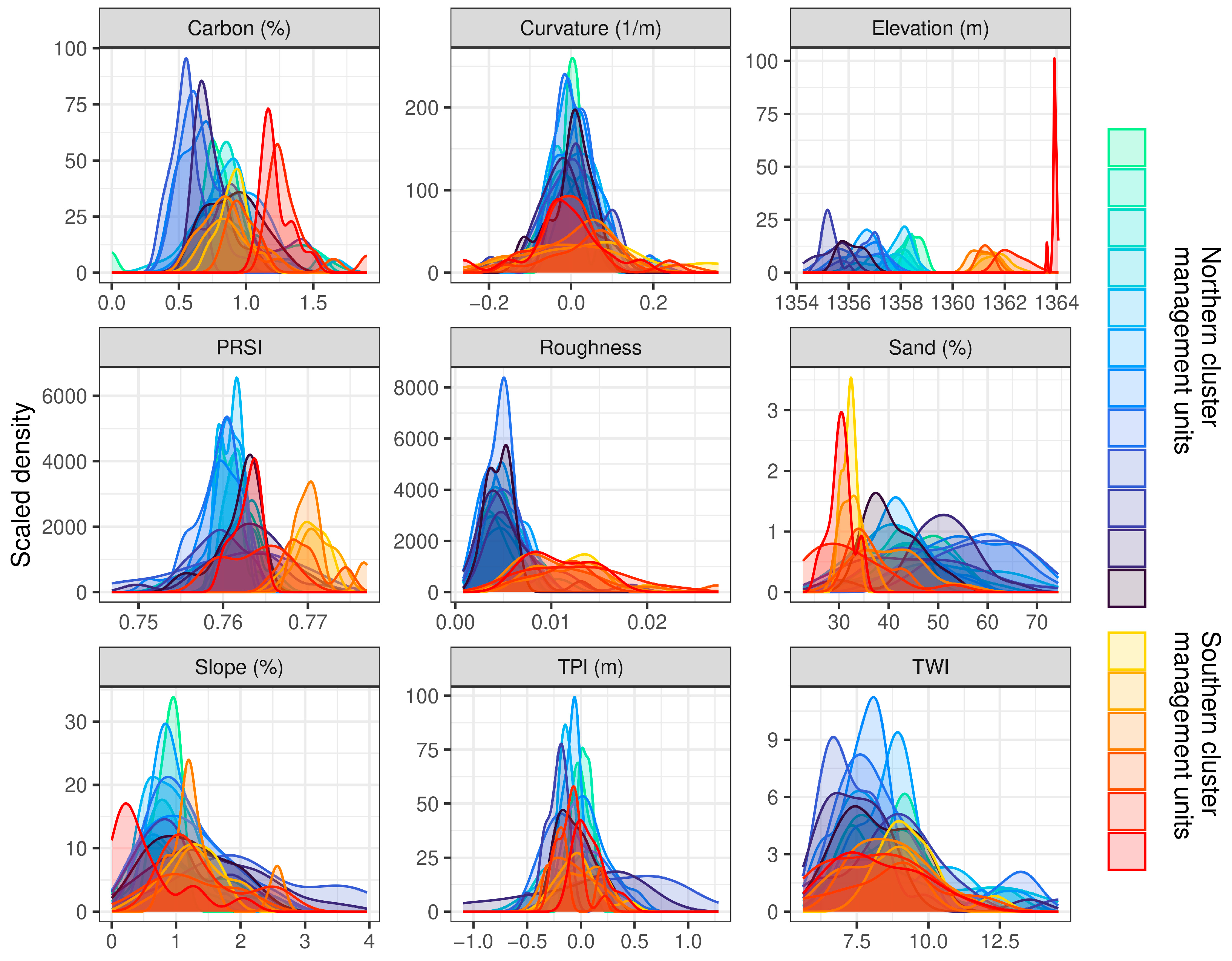
N application rate data were downloaded from the planters (a John Deere 1590 no-till drill for wheat and millet and a John Deere 1700 MaxEmerge Plus planter for corn), equipped with the same model of aftermarket Trimble monitor and integrated display system as the harvester. The raw N application rate data were shapefiles with a series of polygons indicating the application rates and area covered by the planter as it made its way across the field. We created 5 m rasters from these data by extracting N application rate values from the polygons at each cell center.

2.5. Soil Data

Soil cores were collected in either March of 2018 (prior to planting), for management units entering the corn or millet phase of the WCMFx rotation, or in July of 2018, for management units in fallow or entering the wheat phase of either rotation. Soil sampling locations were pre-determined by overlaying a 30 m by 30 m grid of points onto the study site, resulting in a total of 10 to 29 sampling locations per management unit. At each sampling location, 3.2 cm diameter soil cores were collected to a depth of 61 cm. The cores were separated into 0–15 cm, 15–30 cm, and 30–61 cm depth sections. The soil texture and chemistry were analyzed by a commercial lab (Ward Laboratory, Kearney, NE, USA). For full details of soil sampling and processing, see Mikha et al. [29].

2.6. Elevation Data

Elevation data were collected using a real-time kinematic GPS mounted to a vehicle while driving parallel transects spaced 5 m apart. Vertical and horizontal errors of 3 cm or less relative to a local benchmark were attained by this method as verified by cross-validation of the data interpolation method. Elevation data were interpolated to regular 5 m grid digital elevation models (DEMs) using ArcGIS Desktop ArcMap v.10.5 Geostatistical Analyst.

2.7. Predictor Variables

The overarching aim of our modeling effort was to explore how landscape features drive yield. As such, we wanted to test a suite of topographic factors and soil characteristics, while controlling for management factors and interannual differences in yield. At the same time, we wanted to avoid having many highly correlated variables, which would make interpretation of results difficult, and other pitfalls of data dredging. For example, previous work has shown that random forest models may have better predictive accuracy when the number of predators is constrained [45]. Indeed, exploratory analyses showed that for wheat, the fully saturated model with all of the potential predictors that we considered resulted in poorer performance than our final model (spatially blocked cross-validation r2 averaged 17.5%; see Section 2.9 for derivation of performance metric and Section 3.2 for comparison to the final model). Thus, we initially considered many potential predicts, then chose a subset for modeling. Our choice of predictors took into consideration both the correlation structure of the potential predictors (Supplementary Materials S2) and a priori knowledge regarding which variables we hypothesized to be important. This approachallowed us to choose a set of predictors that would represent a wide array of landscape factors with minimal redundancy and allow for interpretation of results rooted in mechanism. All pairwise Pearson correlation coefficients in the final set were <0.6, with the exception of percent sand and percent total soil carbon (r = −0.69).
Because water is the most limiting resource in dryland systems [28,46], it was important to include topographic indices that would reflect patterns of soil water availability. The topographic wetness index (TWI) was included as it correlates with above-ground water runoff and accumulation [47]. The topographic position index (TPI) was included because lower landscape positions likely have higher soil moisture availability due to increased infiltration and below-ground water movement [24,48]. While TWI and TPI (calculated with a 100 m radius) presumably captured the broad patterns of water accumulation within our management units, we reasoned that small depressions and ridges in the landscape may also influence patterns of water runoff and retention. To represent such patterns, we chose to include a metric of surface roughness (sometimes referred to as ruggedness, microrelief, etc.), Roughness Index-Elevation (REI), calculated with the minimum neighborhood size (3 by 3 of our 5 m grid cells). Among the three common curvature metrics, plan, profile, and total curvature, we chose to only include plan curvature as it relates to acceleration and deceleration of surface runoff and may therefore influence infiltration of surface runoff. Slope was included because it was fairly uncorrelated with other potential predictors (with the exception of TWI, r = −0.44); it represented an element of the landscape not well characterized by other metrics, and we believed it may interact with other predictors, mediating the strength of their influence on water movement. The potential solar radiation index (PSRI) was chosen to represent insolation [49]. While elevation can be a problematic variable to use, due to collinearity with factors known to influence yield and lack of transferability, we wanted to include it in our models to test whether or not we would find a consistent relationship between yield and elevation at our study site.
Derivation of the topographic attributes used in the final models is described in Table 3. Surface drainage ditches, which run along some management unit boundaries and along the highway separating two areas of the study site, were built into the DEMs, ensuring that all surface flow was intercepted and routed downstream through these ditches by the flow-routing algorithm in the TWI calculation.
We chose to use total soil carbon at the 0–15 cm depth because previous work at this site showed this variable and depth to be among the most important predictors of winter wheat yield [4]. The Pearson correlation coefficient between soil organic matter and total soil carbon was 0.82. We used the entire 0–61 cm soil profile for sand to represent water holding capacity in the largest portion of the root zone possible. While we did have some pre-planting soil residual NO3 data, it was not included as a modeling variable because it was not sampled in as many locations, as the initial 30 m soil sampling grid collected in 2018, and because there were some time periods in which it was not sampled at all due to logistical constraints.
To account for interannual weather differences, we calculated farm-wide values for the SPEI and growing season precipitation from the onsite weather station. The SPEI was calculated using the R package SPEI [50], using Penman–Monteith potential evapotranspiration for the water balance portion of the calculation. The three-month SPEI was chosen to act as a proxy for near-surface soil moisture at the time of planting [51]. Growing season precipitation was calculated as the cumulative precipitation from the beginning of May to the end of August for corn and millet and from the beginning of May to June 15th for wheat. While the meteorological variables do not vary spatially, they were included in the models to give us a sense of the magnitude of interannual differences in yield which can putatively be assigned to differences in weather.
We included N application rate as a predictor to control for differences in yield due to differential fertilizer application. In the case of the wheat model, we also included a categorical rotation predictor to assess whether there were any differences in yield–predictor relationships, conditional on the two different management systems used to grow wheat in this study.
Finally, categorical predictors for year and management unit were included to account for any large year-to-year or between-management-unit yield differences that were not accounted for by any other variables. This potentially allows for better fitting of the yield–landscape and yield–N relationships within a year or management unit, similar to the inclusion of random effects in a mixed effects model.
Table 3. Topographic variables derived from DEMs, used in random forest models.
VariableAbbreviationUnitsDescription and Derivation
SlopeSlope%Percent slope in direction of maximum slope. Calculated by arcMap extension, TauDEM v.5.3.7 [52].
Potential solar
radiation index
PSRIUnitless P S R I = cos l a t i t u d e cos s l o p e + s i n ( l a t i t u d e )   s i n ( s l o p e )   c o s ( 180 a s c e c t )
where slope is degrees from horizontal.
Profile curvatureCurvaturem−1Curvature in direction of maximum slope. Positive value indicates concave upward. Calculated by ArcGIS Spatial Analyst.
Topographic
wetness index
TWIUnitless T W I = l n F l o w A c c   g r i d   c e l l   a r e a g r i d   c e l l   l e n g t h S l o p e / 100
where FlowAcc is flow accumulation, calculated by TauDEM, using D-infinity flow routing with sinks filled.
Topographic
position index
TPImElevation of focal cell minus mean elevation of a 100 m radius circular neighborhood centered on focal cell. Calculated using the TPI function of the R package MultiscaleDTM version 0.8.3 [53].
Roughness
index-elevation
RoughnessmStandard deviation of residual topography in a 3 by 3 cell focal window, where residual topography is calculated as the focal pixel elevation minus the focal window mean [54]. Calculated using MultiscaleDTM.

2.8. Random Forest Modeling

We modeled yield for each of the three crops separately using random forest regression, as implemented by the R package ranger version 0.17.0 [55] with default hyperparameter settings. The predictor variables used were the N application rate, elevation, 6 DEM-derived topographic variables listed in Table 3, percent sand (0–61 cm), total soil carbon (0–15 cm), 3-month Standardized Precipitation Evapotranspiration Index (SPEI) at the time of planting, and growing season precipitation, as well as categorical variables for year, management unit, and, in the case of wheat, rotation.
We extracted cell values from our 5 m rasters of yield, N application, and topographic attributes at soil sampling locations to create the modeling dataset. Some harvests during the study period exhibited near total crop failure, resulting in uniformly zero-yield values for certain management units in certain years. Because the main focus of our analyses was understanding within-field yield variation, and these management units had no variation, they were removed from the dataset for the years of crop failure. Data from 5 management units were removed (two millet and one corn units for 2020, one millet unit for 2021, and one corn unit for 2022), leaving us with data from 22 wheat harvests, 10 corn harvests, and 9 millet harvests.

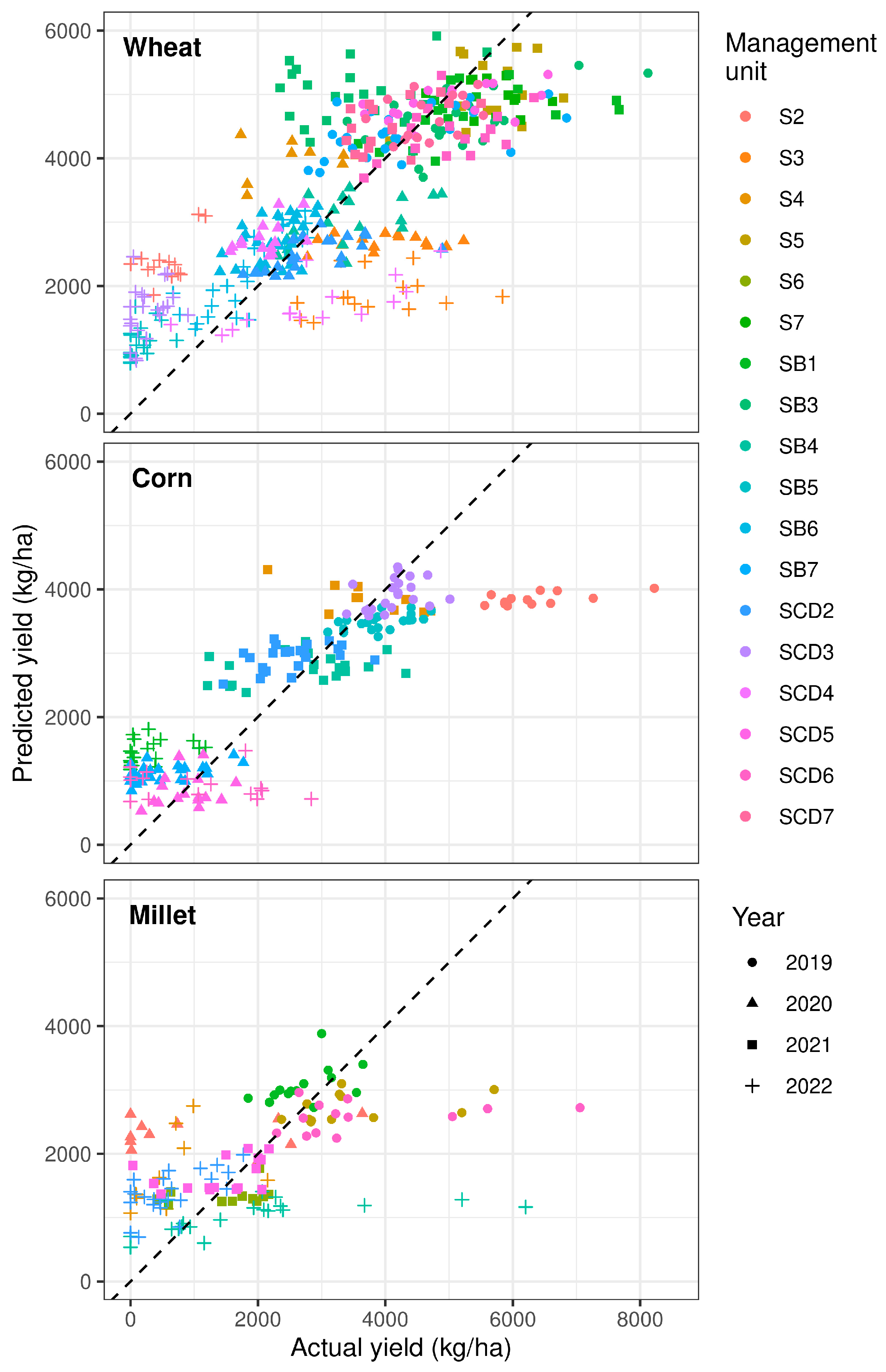
2.9. Evaluating Model Performance

We used blocked cross-validation [35] to evaluate the models on hold-out data, designating each management unit as a different block. While our data are strongly temporally correlated, we chose not to block with respect to time, because we are less interested in testing our models’ ability to predict farm-wide interannual yield differences than we are to test the ability of predicting within-field spatial variability. Additionally, blocking by both time and space would have reduced the training datasets to such small subsets of the data that parameter fits would have potentially become unstable. To illustrate the importance of using blocked data for model evaluation, we also calculated model performance employing a typical, but inappropriate, method of 10-fold cross-validation with data points assigned to folds randomly. We used the coefficient of determination (r2) between predicted and actual data as our metric of model performance.

2.10. Calculating Effect Sizes and Significance

To test whether the direction and magnitude of our predictors’ effects on yield were consistent from management unit to management unit, we calculated effect sizes and bootstrapped confidence intervals from the random forest models, following the methods of Cafri and Bailey [56]. In this method, the coefficient estimates from a linear model, fit to the partial dependence values for a given predictor, are considered a point estimate of the effect size. Confidence intervals for the effect size are constructed by creating multiple bootstrap samples from the dataset and calculating an effect size point estimate for each. Our bootstrapped samples were constructed by blocking the data by management unit and then sampling n blocks with replacement, where n is the total number of total units available. A total of 1000 bootstrap iterations were performed. This procedure was carried out for all predictors with within-management-unit spatial variability. Variables were considered significant if the 95% confidence interval did not cross zero.

3. Results

3.1. Data Summaries

Yield exhibited a high degree of spatial and temporal variation for all three crops (Figure 3). Across all management units, the yearly mean yield ranged from 1443 to 4837 kg/ha for wheat, 611 to 4574 kg/ha for corn, and 863 to 3182 kg/ha for millet. Within a year, the inter-management unit standard deviation in yield averaged 893 kg/ha, 733 kg/ha, and 452 kg/ha for wheat, corn, and millet, respectively, while the intra-management unit standard deviation averaged 739 kg/ha, 595 kg/ha, and 914 kg/ha for wheat, corn, and millet, respectively.
The distribution of soil properties and topographic data used for modeling is shown for all management units in Figure 4. Across all management units, total soil carbon was very low, with a mean of 0.86% and a standard deviation of 0.27%. Percent sand had a large degree of variability, ranging from 22.6% to 74.3%. Overall topographic relief and distributions of topographic derived indices were low, with the exception of the TWI, which tends to increase in areas with small slopes. Elevation had a mean of 1358 m and a standard deviation of 2.5 m, the TPI had a mean of 0.0 m and a standard deviation of 0.3 m, slope had a mean of 1.2% and a standard deviation of 0.7%, and the TWI had a mean of 8.4 with a standard deviation 1.61, but ranged as high as 14.5.

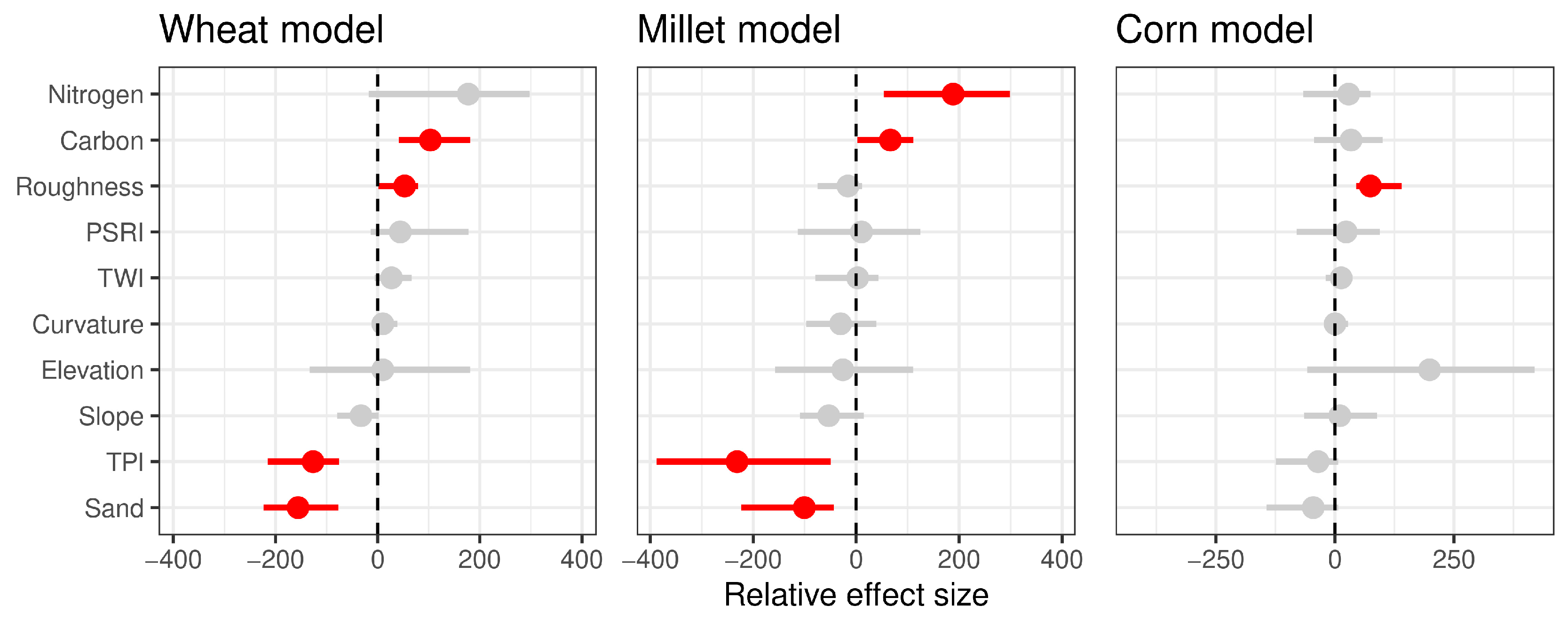
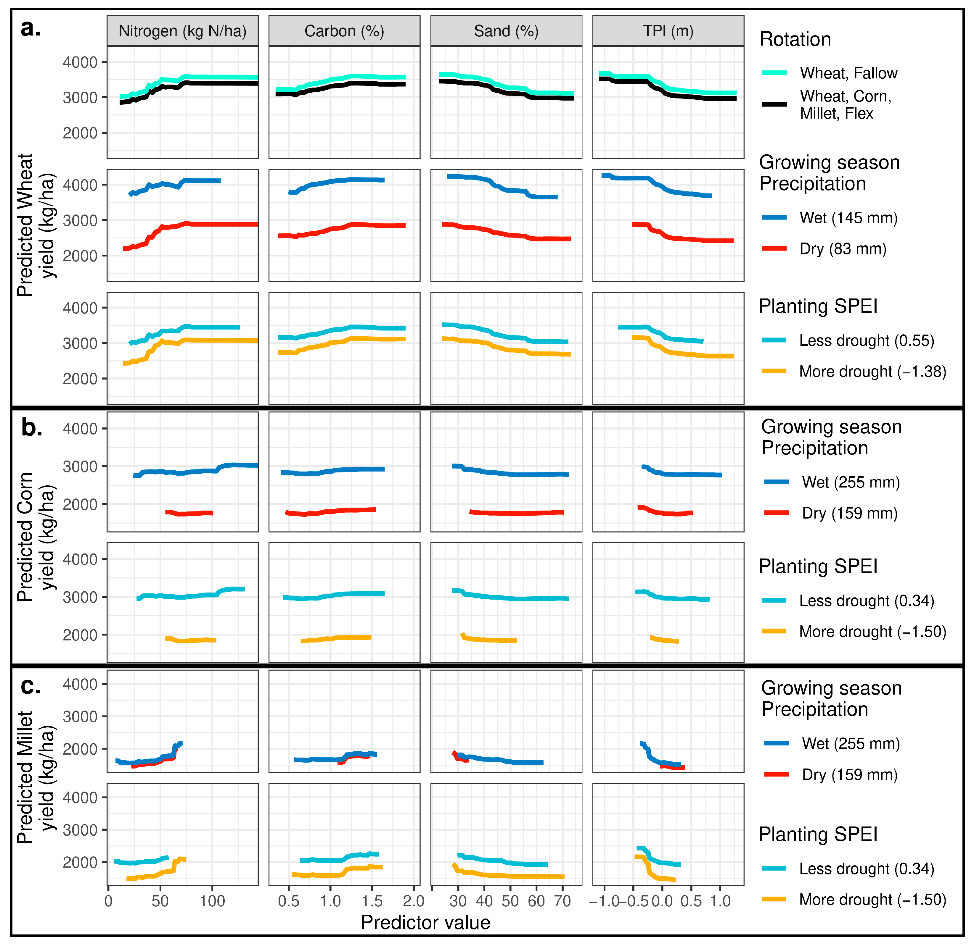
3.2. Modeling Results

The random forest models’ out-of-bag errors (pseudo R2, estimated without spatial blocked cross-validation) were 0.86 for wheat, 0.91 for corn, and 0.58 for millet. The variance explained for testing data (r2) using a typical approach of random 10-fold cross-validation yielded similar model performance to that of training data, with r2 values averaging 0.87 for the wheat model, 0.91 for corn, and 0.60 for millet. However, when the models were tested, using spatially blocked cross-validation to reduce statistical dependence between training and testing data, model performance decreased substantially. The mean r2 was 0.25 for the wheat model, 0.21 for corn, and 0.19 for millet. Predicted versus actual yield values for the withheld block (i.e., management unit) from each cross-validation iteration are shown in Figure 5.
Permutation variable importance scores as measured by the percent-increase root mean squared error are shown in Table 4. The significant predictors of yield were the TPI, percent sand, and total soil carbon for the wheat and millet models; N application for the millet model only; and roughness for the wheat and corn models (Figure 6). The variables with the largest effect on yield for wheat and millet were the N application rate, TPI, percent sand, and total soil carbon.
Predicted wheat yield varied by approximately 750 kg/ha over the range of N values present in the dataset (Figure 7a, first column). Predicted wheat yield varied by approximately 600 kg/ha over the range of TPI values present in the dataset (Figure 7a, fourth column), and 600 kg/ha over the range of percent sand values present in the dataset (Figure 7a, third column). Predicted wheat and corn yield both varied by a little over 1000 kg/ha between a year with low growing season precipitation and a year with high precipitation (Figure 7a, second row, and Figure 7b, first row, respectively). We examined partial dependence plots qualitatively for evidence of interactive effects between the four strongest predictors and rotation (i.e., differing slopes between the WF and WCMFx partial dependence curves), but the differences were negligible, if any (Figure 7a, first row).

4. Discussion

To better understand within-field yield variability, we collected high-resolution topographic, soil texture and chemistry, N application rate, weather, and yield data over 4 years and 18 management units at a research farm employing dryland cultural practices in a semi-arid region. We modeled yield for each of the three crop types present in the study separately using random forest regression. As expected, we found a high degree of both temporal and spatial yield variability for all three crops (Figure 3). While there was substantial interannual and between-management-unit variation in yield, we were most interested in factors affecting within-management-unit spatial variation in yield. Of the predictors that varied spatially, some differed in terms of the direction, shape, and magnitude of their relationship with yield between the three crops. However, a few were consistent among crops in terms of direction and tended to have large effect sizes. The TPI and percent sand tended to have a strong negative effect on yield, while the N application rate and total soil carbon tended to have a strong positive effect on yield (Figure 6). Over the range of values present in the dataset, each of these four predictors caused a variation of at least 500 kg/ha in predicted wheat yield, or >15% of the overall mean wheat yield. For millet, each of these predictors caused at least 400 kg/ha of variation in predicted yield, or >22% of the overall mean yield.

4.1. Effects of Topography

Remarkably, the TPI had almost as strong of an effect on yield as N application rate (Figure 6). In the wheat model for example, yield varied by approximately 600 kg/ha over the range of TPI values present in the dataset (Figure 7a, fourth column), only slightly less than the 750 kg/ha range of predicted values due to N (Figure 7a, first column). This result, which indicates that local depressions are expected to produce substantially higher yields than higher landscape positions, is likely driven largely by spatial variation in water availability. The TPI is correlated with water availability due to the combined influence of the finer soil texture in low-lying areas [18,21], surface runoff, below-ground lateral water flow [24], differential infiltration rates associated with landscape position [48], and differential vertical drainage rates associated with topographic position [57]. Higher topographic positions are also likely to lose topsoil due to erosion over time. This exposes deeper soils that have higher concentrations of calcium carbonate [58], resulting in decreased productivity in higher topographic positions and increased productivity in lower topographic positions.
Very few studies have used the TPI as a predictor of yield. Of the two studies we are aware of that did so, one found the TPI to be very strongly correlated with yield (r = −0.74), more so than elevation (r = −0.54), which is consistent with our results [59]. The other found that the inclusion of the TPI improved model accuracy slightly relative to models based on spectral indices alone, but made no mention of the nature of the yield–TPI relationship [38]. An additional study used a similar metric that indicated whether a focal cell was high or low relative to a neighborhood around it, which they termed “relative elevation,” and found it to be among their best single predictors, but again, they made no mention of the nature of its relationship with yield [14]. Finally, Martinez-Feria and Basso [3] used the TPI to categorize areas within fields into discrete landscape positions and then looked for associations between landscape positions and interannual yield stability. They found that the highest and lowest landscape positions were more likely to have unstable yields across years and concluded that local high positions had lower-than-field-average yield in dry years due to water deficits and that local low positions had lower-than-field-average yield in wet years due to water excess. These findings corroborate our own in terms of the TPI mediating water availability to influence yield. They also highlight the need for an improved understanding of the mechanisms underlying yield–predictor relationships, as the nature of such relationships may change from year to year and site to site.
It is noteworthy that the TPI performed much better than the TWI in our study, yet the TWI is a very commonly used, topographically derived proxy for water availability. The flow accumulation algorithms used in the calculation of the TWI tend to create very channelized flow lines that may not be realistic in areas with gentle topography. The TPI often produces similar spatial patterns to (the inverse of) the TWI, but without the unrealistically stark contrasts between flow accumulation lines and areas immediately adjacent to flow accumulation lines (e.g., Figure 8f,g). Marques Da Silva and Silva [19] found that distance to flow accumulation lines was a better predictor of corn yields than either the TWI or flow accumulation itself, suggesting that soil moisture (or any other property driving yield) does not drop off immediately outside of flow paths. Additionally, in very flat areas, the near-zero slope values in the denominator of the TWI calculation (Table 3) make the term inside the logarithm asymptotically approach infinity, resulting in unstable and unrealistically heterogeneous TWI values (e.g., Figure 8b). Therefore, the TWI can be a fraught metric to use in systems that typically have very flat areas, such as agricultural fields.
It may be possible to minimize unproductive inputs or even mitigate the strength of the negative effect of the TPI on yield by reducing seeding rates in upper landscape positions, thereby reducing competition for water in the most water-limited parts of the field [60,61]. Alternatively, recent work has revealed the potential economic and environmental benefits of fine-scale conservation plantings in consistently low-yielding zones within fields [10]. Locations with high TPI values may be good candidates for such targeted conservation treatments in arid systems, if such areas consistently produce very low or negative profit margins for all crops in the rotation.
Finally, it is worth noting that elevation, despite being a moderately important variable as measured by permutation variable importance scores (Table 4) for the dataset as a whole, did not have a consistent direction of effect on yield when trained on different subsets of management units (Figure 6). Fields typically have some gradient in elevation and some variation in yield, so machine learning models will generally be able to fit a relationship between the two. However, as our results show, the relationship will not necessarily be transferable from site to site, or even from location to location, within the same farm. These results illustrate how easy it is to overfit machine learning models when using spatial data and how important it is to test models on data that is spatially separated from training data.

4.2. Effects of Nitrogen

Of the predictors that varied spatially, the N application rate had the largest effect on wheat yields and the second largest effect on millet yields (Figure 6). Despite the large effect size, the N application rate was not statistically significant in the wheat model. This is simply due to the fact that the wheat management units using the WF rotation had uniform N application target rates within units. Therefore, bootstrap iterations that sampled mainly WF units would not have been likely to find a relationship between N and yield. We found no evidence of an interactive effect between N and management practice (Figure 7a, first row). In other words, wheat yields responded equally strongly to N application despite differences in tillage and crop rotation between the WF and WCMFx management units. We cannot rule out the possibility that the lack of difference in N response between management practices is due to data limitations, however. Similarly to the lack of N response found in certain bootstrap iterations, the dataset as a whole may have lacked sufficient coverage of predictor space in terms of N application rates in WF management units to fit an accurate N response curve. A dataset from an experiment that includes all permutations of low-through-high N application rates, in both management systems across multiple years, would allow for more robust model fitting results and is a recommended goal for future research.

4.3. Effects of Soil Characteristics

Soil texture is also a strong driver of within-field yield variability. Similarly to previous studies [2,4], we found percent sand to have a substantial negative association with yield (Figure 6). For example, in a year with dry planting conditions, millet is predicted to produce nearly 500 kg/ha less yield in a location with 50% sand than in a location with 28% sand (Figure 7c, second row, third column). This relationship is likely driven by lower water, cation exchange [62], and nutrient holding capacity [63] in sandier soils.
Total soil carbon had a positive relationship of moderate effect size with yield in the wheat and millet models. Soils at this study site are characterized by very low total soil carbon (0.3 to 1.9%) and low organic matter (0.6 to 4.0%). Soil carbon affects several factors with the potential to positively affect yield, including increased plant available water capacity, N, P, and S availability, and increased cation exchange capacity [64]. Care must be taken when drawing conclusions as to the directionality and mechanisms underlying the carbon–yield relationship, however. First, carbon may be collinear with topographic and hydrologic attributes [65]. Second, inherently more fertile areas in the landscape may have higher net primary productivity, driving increased soil carbon, or creating a positive feedback between the two [66,67]. The positive association between soil carbon and yield suggests an opportunity to increase crop performance with management practices that boost soil carbon, such as organic amendments or alterations to tillage and fallow regimes, but the efficacy of such treatments will depend on specific mechanisms responsible for the carbon–yield relationship.

4.4. Model Performance

Our model performance compares favorably with that of many previous studies in terms of variance explained for training data (e.g., [34,37,38]). We improved the wheat model pseudo R2 value from previous work at this study site considerably, from 28% to 86%, by including topographic attributes and a larger dataset (compared to Ramirez et al. [4]). Yet a key omission from the majority of studies on yield spatial variability is the evaluation of model performance on statistically independent (i.e., spatially distinct) testing data. When cross-validated on spatially blocked data, our models only explained approximately one-quarter of the within-management-unit yield variance. Similarly, Liu et al. [68] found large decreases in model performance when applying an artificial neural network model of corn yield to data that was spatially independent from their training set. These findings are important because they suggest that previous modeling work reporting variance explained without evaluation of model performance on independent testing data must be interpreted with caution.
Few studies that we are aware of achieved strong model performance on independent testing data. Of these, all used spectral indices collected mid-growing season (e.g., [1]). This aligns with expectations that such models predict yield well, given that indices such as the NDVI are well-established indicators of crop yield [69,70,71]. We chose not to include spectral indices in our models because we were more interested in the underlying landscape factors that presumably drive similar spatial patterns in both yield and spectral indices, rather than maximizing model prediction metrics. We also argue that the development of models that do not rely on mid-season data collection is important, because most management decisions in dryland systems are made at the time of planting. While our models do include growing season precipitation, its inclusion was simply to allow better model fitting in terms of interannual differences in yield–predictor relationships, rather than to guide mid-season management decisions. Nonetheless, remotely sensed spectral data collected mid-season do offer an opportunity to investigate the performance of crops throughout their development with an exceptionally high spatial and temporal resolution, making them a promising avenue for future research.

4.5. Sources of Unexplained Variance and Directions for Future Work

A large portion of the yield variation that our models were unable to capture was likely caused by spatial variability in precipitation. Published work in eastern Colorado has found fine-scale (<2 km; similar in size to our study site) differences among rain gauges ranging from approximately 10 mm to 28 mm over the growing season [72]. Variation in precipitation could be even greater for individual storms, which could drive substantial variation in yield if they occur during the points in the growing season in which water availability is most critical. Given the fact that precipitation during critical time windows can have a large impact on yield [27,73] and the generally strong responsiveness of yield to water use shown at our study site previously [74], it is plausible that spatial variation in precipitation could account for a large portion of our unexplained yield variation.
Water is the most limiting resource in dryland systems [28,46]. Several of our yield–predictor relationships (the TPI, TWI, and percent sand) are consistent with the idea that spatial variability in water availability is one of the greatest factors driving yield variability, in agreement with Martinez-Feria and Basso [3]. However, our predictors are only a rough proxy for soil moisture. Much of the unexplained variance in our models could be accounted for by the imperfect relationships between our predictors and true soil moisture. Future work that measures soil moisture directly at high spatial and temporal resolutions will help confirm our interpretation and will clarify what proportion of yield variation can be explained by soil moisture variation. Quantifying soil moisture–yield relationships directly will be especially helpful for producing models that are transferable across sites, as the relationships between proxies for soil moisture (i.e., topography and soil properties) and soil moisture itself could differ from system to system. Spatially distributed process-based hydrologic models could also be employed to gain insights into the spatial and temporal dynamics of yield–soil moisture relationships. We also acknowledge that landscape factors are unlikely to explain 100% of yield variation and that management decisions such as crop type, rotation, and fertilizer application are larger drivers. Nonetheless, this study advances understanding by being the first of its kind to address what ranges of variance explained may be attributable solely to landscape factors while generally accounting for precipitation and broader management decisions.
Ultimately, the strongest evidence of the mechanistic processes driving yield will come from experimentation. Heterogeneity in the landscape and weather create spatial and temporal dynamics of water availability that are difficult, if not impossible, to approximate through topographic proxies or hydrologic modeling. Because of this, experiments should directly manipulate soil moisture at the replicate scale to ensure that differences in water availability are neither confounding, nor interacting with treatment effects. In cases when such manipulations are infeasible, stratifying experimental blocks by the TPI or distance to flow paths may be a better approach to controlling for water availability than stratifying by the TWI. Future work will benefit from combining observational datasets, such as that used in the present study, with experimental studies that can infer causation. Indeed, machine learning analyses of observational datasets that show non-linear relationships and variable interactions are quite powerful in helping drive the formation of hypotheses to be later tested via experimentation.
The accuracy of our yield monitor data likely accounts for some of the unexplained variance in our models. The scale of the landscape features and corresponding yield patterns that we measured in the present study may be too small to be accurately captured by yield monitors. Gauci et al. [75] created plots of varying sizes that intentionally alternated between high and low corn yields and then assessed multiple yield monitors’ ability to detect differences between plots, as well as the accuracy of yield estimates within plots. All four of the tested monitors failed to detect yield differences across plots that were less than 43 m in length, and the monitors did not accurately capture the magnitude of yield within plots that were less than 60 m in length. Furthermore, one of the monitors had highly variable readings within plots and tended to overestimate yield in the high-yield plots. Harvester speed and inclination can also affect yield monitor readings [2]. Future work should consider weighing yield from discrete plots of a fixed area, rather than relying on the continuous mass flow sensor data from yield monitors.

5. Conclusions

This study utilized an extensive multiyear dataset with uniquely high-resolution sampling of soil properties, in a dryland system, to better understand drivers of within-field yield variability. We found the TPI to be the best topographic predictor of yield. It outperformed the TWI, possibly because it is a better proxy for soil moisture in low-relief settings, and it is a transferable metric from site to site, unlike elevation. The nitrogen application rate, soil texture, and soil carbon also had strong influences on yield. Despite the size and quality of our dataset, we found that when evaluated appropriately, our models explained only one-quarter of within-management-unit yield variance. However, we acknowledge it is unrealistic to expect landscape features alone to explain the entirety of crop yield variance. We instead point to the limited explanatory power of our models being constrained by increased data needs in capturing landscape responses. Future studies that better characterize the spatial variability of water availability, interactive effects of weather, and carefully designed experiments may increase our ability to explain spatial and temporal yield variability.

Supplementary Materials

The following supporting information can be downloaded at: https://www.mdpi.com/article/10.3390/agronomy15061304/s1, Supplement S1: Yield data quality control and processing. Supplement S2: Correlation plot of potential predictor variables. Supplement S3: Yield and predictor maps. Supplement S4: Scatterplot relationships between yield and predictor variables.

Author Contributions

Conceptualization, K.R.M., D.M.B., and J.A.M.; Methodology, J.A.M., D.M.B., and R.H.E.; Formal Analysis, J.A.M. and R.H.E.; Investigation, D.J.P., R.H.E., and M.M.M.; Resources, D.J.P.; Data Curation, J.A.M., D.J.P., and R.H.E.; Writing—Original Draft Preparation, J.A.M., K.R.M., D.M.B., G.L.M., and R.H.E.; Writing—Review and Editing, J.A.M., K.R.M., D.M.B., G.L.M., R.H.E., A.L.M., S.M., D.J.P., and M.M.M.; Visualization, J.A.M.; Supervision, K.R.M. and D.M.B.; Project Administration, K.R.M. and D.M.B. All authors have read and agreed to the published version of the manuscript.

Funding

This research was funded by the USDA Agricultural Research Service.

Data Availability Statement

The data presented in this study are publicly available at https://doi.org/10.5281/zenodo.15519944.

Acknowledgments

This research was supported by the USDA Agricultural Research Service. The USDA is an equal opportunity provider, employer, and lender.

Conflicts of Interest

The authors declare no conflicts of interest.

Abbreviations

The following abbreviations are used in this manuscript:
DEMDigital elevation model
NNitrogen
PPhosphorus
PSRIPotential solar radiation index
SPEIStandardized Precipitation Evapotranspiration Index
TPITopographic position index
TWITopographic wetness index
WFWheat–fallow rotation
WCMFxWheat–corn–millet–flexible planting decision rotation

References

  1. Fiorentini, M.; Schillaci, C.; Denora, M.; Zenobi, S.; Deligios, P.; Orsini, R.; Santilocchi, R.; Perniola, M.; Montanarella, L.; Ledda, L. A Machine Learning Modeling Framework for Triticum turgidum Subsp. Durum Desf. Yield Forecasting in Italy. Agron. J. 2024, 116, 1050–1070. [Google Scholar] [CrossRef]
  2. Iqbal, J.; Read, J.J.; Thomasson, A.J.; Jenkins, J.N. Relationships between Soil–Landscape and Dryland Cotton Lint Yield. Soil Sci. Soc. Am. J. 2005, 69, 872–882. [Google Scholar] [CrossRef]
  3. Martinez-Feria, R.A.; Basso, B. Unstable Crop Yields Reveal Opportunities for Site-Specific Adaptations to Climate Variability. Sci. Rep. 2020, 10, 2885. [Google Scholar] [CrossRef] [PubMed]
  4. Ramírez, P.B.; Calderón, F.J.; Vigil, M.F.; Mankin, K.R.; Poss, D.; Fonte, S.J. Dryland Winter Wheat Production and Its Relationship to Fine-Scale Soil Carbon Heterogeneity—A Case Study in the US Central High Plains. Agronomy 2023, 13, 2600. [Google Scholar] [CrossRef]
  5. Nielsen, D.C.; Vigil, M.F.; Hansen, N.C. Evaluating Potential Dryland Cropping Systems Adapted to Climate Change in the Central Great Plains. Agron. J. 2016, 108, 2391–2405. [Google Scholar] [CrossRef]
  6. Bongiovanni, R.; Lowenberg-Deboer, J. Precision Agriculture and Sustainability. Precis. Agric. 2004, 5, 359–387. [Google Scholar] [CrossRef]
  7. Pierce, F.J.; Nowak, P. Aspects of Precision Agriculture. In Advances in Agronomy; Elsevier: Amsterdam, The Netherlands, 1999; pp. 1–85. ISBN 0065-2113. [Google Scholar]
  8. Kharel, T.P.; Maresma, A.; Czymmek, K.J.; Oware, E.K.; Ketterings, Q.M. Combining Spatial and Temporal Corn Silage Yield Variability for Management Zone Development. Agron. J. 2019, 111, 2703–2711. [Google Scholar] [CrossRef]
  9. Karunathilake, E.M.B.M.; Le, A.T.; Heo, S.; Chung, Y.S.; Mansoor, S. The Path to Smart Farming: Innovations and Opportunities in Precision Agriculture. Agriculture 2023, 13, 1593. [Google Scholar] [CrossRef]
  10. Adhikari, K.; Smith, D.R.; Hajda, C.; Kharel, T.P. Within-Field Yield Stability and Gross Margin Variations across Corn Fields and Implications for Precision Conservation. Precis. Agric 2023, 24, 1401–1416. [Google Scholar] [CrossRef]
  11. Kravchenko, A.N.; Robertson, G.P.; Thelen, K.D.; Harwood, R.R. Management, Topographical, and Weather Effects on Spatial Variability of Crop Grain Yields. Agron. J. 2005, 97, 514–523. [Google Scholar] [CrossRef]
  12. Cox, M.S.; Gerard, P.D. Soil Management Zone Determination by Yield Stability Analysis and Classification. Agron. J. 2007, 99, 1357–1365. [Google Scholar] [CrossRef]
  13. Nawar, S.; Corstanje, R.; Halcro, G.; Mulla, D.; Mouazen, A.M. Delineation of Soil Management Zones for Variable-Rate Fertilization. In Advances in Agronomy; Elsevier: Amsterdam, The Netherlands, 2017; Volume 143, pp. 175–245. ISBN 978-0-12-812421-5. [Google Scholar]
  14. Rampant, P.; Abuzar, M. Geophysical Tools and Digital Elevation Models: Tools for Understanding Crop Yield and Soil Variability. In Proceedings of the SuperSoil 2004: 3rd Australian New Zealand Soils Conference, Sydney, Australia, 5–9 December 2004. [Google Scholar]
  15. Liebig, M.A.; Franzluebbers, A.J.; Alvarez, C.; Chiesa, T.D.; Lewczuk, N.; Piñeiro, G.; Posse, G.; Yahdjian, L.; Grace, P.; Cabral, O.M.R.; et al. MAGGnet: An International Network to Foster Mitigation of Agricultural Greenhouse Gases. Carbon Manag. 2016, 7, 243–248. [Google Scholar] [CrossRef]
  16. Ferrara, R.M.; Trevisiol, P.; Acutis, M.; Rana, G.; Richter, G.M.; Baggaley, N. Topographic Impacts on Wheat Yields under Climate Change: Two Contrasted Case Studies in Europe. Theor. Appl. Clim. 2010, 99, 53–65. [Google Scholar] [CrossRef]
  17. Erskine, R.H.; Green, T.R.; Ramirez, J.A.; MacDonald, L.H. Digital Elevation Accuracy and Grid Cell Size: Effects on Estimated Terrain Attributes. Soil Sci. Soc. Am. J. 2007, 71, 1371–1380. [Google Scholar] [CrossRef]
  18. Kumhálová, J.; Kumhála, F.; Kroulík, M.; Matějková, Š. The Impact of Topography on Soil Properties and Yield and the Effects of Weather Conditions. Precis. Agric. 2011, 12, 813–830. [Google Scholar] [CrossRef]
  19. Marques Da Silva, J.R.; Silva, L.L. Evaluation of the Relationship between Maize Yield Spatial and Temporal Variability and Different Topographic Attributes. Biosyst. Eng. 2008, 101, 183–190. [Google Scholar] [CrossRef]
  20. Rodriguez Miranda, D.A.; De Oliveira Alari, F.; Oldoni, H.; Bazzi, C.L.; Do Amaral, L.R.; Graziano Magalhães, P.S. Delineation of Management Zones in Integrated Crop–Livestock Systems. Agron. J. 2021, 113, 5271–5286. [Google Scholar] [CrossRef]
  21. Li, Y.; Lindstrom, M.J. Evaluating Soil Quality–Soil Redistribution Relationship on Terraces and Steep Hillslope. Soil Sci. Soc. Am. J. 2001, 65, 1500–1508. [Google Scholar] [CrossRef]
  22. Cox, M.S.; Gerard, P.D.; Abshire, M.J. Selected soil properties’ variability and their relationships with yield in three Mississippi fields. Soil Sci. 2006, 171, 541–551. [Google Scholar] [CrossRef]
  23. Rabia, A.H.; Neupane, J.; Lin, Z.; Lewis, K.; Cao, G.; Guo, W. Principles and Applications of Topography in Precision Agriculture. In Advances in Agronomy; Elsevier: Amsterdam, The Netherlands, 2022; pp. 143–189. ISBN 0065-2113. [Google Scholar]
  24. McCord, J.T.; Stephens, D.B. Lateral Moisture Flow beneath a Sandy Hillslope without an Apparent Impeding Layer. Hydrol. Process. 1987, 1, 225–238. [Google Scholar] [CrossRef]
  25. Nielsen, D.C.; Unger, P.W.; Miller, P.R. Efficient Water Use in Dryland Cropping Systems in the Great Plains. Agron. J. 2005, 97, 364–372. [Google Scholar] [CrossRef]
  26. Couëdel, A.; Edreira, J.; Lollato, R.; Archontoulis, S.; Sadras, V.; Grassini, P. Assessing Environment Types for Maize, Soybean, and Wheat in the United States as Determined by Spatio-Temporal Variation in Drought and Heat Stress. Agric. For. Meteorol. 2021, 307, 108513. [Google Scholar] [CrossRef]
  27. Miner, G.L.; Stewart, C.E.; Vigil, M.F.; Poss, D.J.; Haley, S.D.; Jones-Diamond, S.M.; Mason, R.E. Does Agroecosystem Management Mitigate Historic Climate Impacts on Dryland Winter Wheat Yields? Agron. J. 2022, 114, 3515–3530. [Google Scholar] [CrossRef]
  28. Wan, C.; Dang, P.; Gao, L.; Wang, J.; Tao, J.; Qin, X.; Feng, B.; Gao, J. How Does the Environment Affect Wheat Yield and Protein Content Response to Drought? A Meta-Analysis. Front. Plant Sci. 2022, 13, 896985. [Google Scholar] [CrossRef]
  29. Mikha, M.M.; Mankin, K.R.; Khan, S.B.; Barnard, D.M. Precision Management Influences Productivity and Nutrients Availability in Dryland Cropping System. Agron. J. 2024, 116, 3325–3343. [Google Scholar] [CrossRef]
  30. Kravchenko, A.N.; Bullock, D.G.; Boast, C.W. Joint Multifractal Analysis of Crop Yield and Terrain Slope. Agron. J. 2000, 92, 1279–1290. [Google Scholar] [CrossRef]
  31. Chi, B.-L.; Bing, C.-S.; Walley, F.; Yates, T. Topographic Indices and Yield Variability in a Rolling Landscape of Western Canada. Pedosphere 2009, 19, 362–370. [Google Scholar] [CrossRef]
  32. Breiman, L. Random Forests. Mach. Learn. 2001, 45, 5–32. [Google Scholar] [CrossRef]
  33. Ziegler, A.; König, I.R. Mining Data with Random Forests: Current Options for Real-world Applications. WIREs Data Min. Knowl. Discov. 2014, 4, 55–63. [Google Scholar] [CrossRef]
  34. Leo, S.; De Antoni Migliorati, M.; Grace, P.R. Predicting Within-field Cotton Yields Using Publicly Available Datasets and Machine Learning. Agron. J. 2021, 113, 1150–1163. [Google Scholar] [CrossRef]
  35. Roberts, D.R.; Bahn, V.; Ciuti, S.; Boyce, M.S.; Elith, J.; Guillera-Arroita, G.; Hauenstein, S.; Lahoz-Monfort, J.J.; Schröder, B.; Thuiller, W.; et al. Cross-validation Strategies for Data with Temporal, Spatial, Hierarchical, or Phylogenetic Structure. Ecography 2017, 40, 913–929. [Google Scholar] [CrossRef]
  36. Koutsos, T.M.; Menexes, G.C.; Mamolos, A.P. The Use of Crop Yield Autocorrelation Data as a Sustainable Approach to Adjust Agronomic Inputs. Sustainability 2021, 13, 2362. [Google Scholar] [CrossRef]
  37. Miao, Y.; Mulla, D.J.; Robert, P.C. Identifying Important Factors Influencing Corn Yield and Grain Quality Variability Using Artificial Neural Networks. Precis. Agric 2006, 7, 117–135. [Google Scholar] [CrossRef]
  38. Oliveira, M.F.D.; Ortiz, B.V.; Morata, G.T.; Jiménez, A.-F.; Rolim, G.D.S.; Silva, R.P.D. Training Machine Learning Algorithms Using Remote Sensing and Topographic Indices for Corn Yield Prediction. Remote Sens. 2022, 14, 6171. [Google Scholar] [CrossRef]
  39. Soil Survey Staff. Soil Taxonomy: A Basic System of Soil Classification for Making and Interpreting Soil Surveys, Natural Resources Conservation Service. In Agricultural Handbook 436; Natural Resources Conservation Service: Washington, DC, USA; USDA: Washington, DC, USA, 1999; Volume 17, p. 869. [Google Scholar]
  40. Soil Survey Staff. Web Soil Survey, National Resources Conservation Service; United States Department of Agriculture: Washington, DC, USA, 2024.
  41. Nielsen, D.C.; Vigil, M.F.; Benjamin, J.G. Evaluating Decision Rules for Dryland Rotation Crop Selection. Field Crops Res. 2011, 120, 254–261. [Google Scholar] [CrossRef]
  42. Hergert, G.W.; Shaver, T.M. Fertilizing Winter Wheat (EC143); University of Nebraska-Lincoln Extension: Lincoln, NE, USA, 2009. [Google Scholar]
  43. Shapiro, C.A.; Ferguson, R.B.; Wortmann, C.S.; Maharjan, B.; Krienke, B. Nutrient Management Suggestions for Corn (EC117); University of Nebraska-Lincoln Extension: Lincoln, NE, USA, 2019. [Google Scholar]
  44. Blumenthal, J.M.; Baltensperger, D.D. Fertilizing Proso Millet (G89-924); University of Nebraska-Lincoln Extension: Lincoln, NE, USA, 2002. [Google Scholar]
  45. Barnard, D.M.; Germino, M.J.; Pilliod, D.S.; Arkle, R.S.; Applestein, C.; Davidson, B.E.; Fisk, M.R. Cannot See the Random Forest for the Decision Trees: Selecting Predictive Models for Restoration Ecology. Restor. Ecol. 2019, 27, 1053–1063. [Google Scholar] [CrossRef]
  46. Connor, D.J.; Loomis, R.S.; Cassman, K.G. Crop Ecology: Productivity and Management in Agricultural Systems, 2nd ed.; Cambridge University Press: Cambridge, UK, 2011; ISBN 978-0-521-76127-7. [Google Scholar]
  47. Beven, K.J.; Kirkby, M.J. A Physically Based, Variable Contributing Area Model of Basin Hydrology/Un Modèle à Base Physique de Zone d’appel Variable de l’hydrologie Du Bassin Versant. Hydrol. Sci. Bull. 1979, 24, 43–69. [Google Scholar] [CrossRef]
  48. Green, T.R.; Dunn, G.H.; Erskine, R.H.; Salas, J.D.; Ahuja, L.R. Fractal Analyses of Steady Infiltration and Terrain on an Undulating Agricultural Field. Vadose Zone J. 2009, 8, 310–320. [Google Scholar] [CrossRef]
  49. Keating, K.A.; Gogan, P.J.P.; Vore, J.M.; Irby, L.R. A Simple Solar Radiation Index for Wildlife Habitat Studies. J. Wildl. Manag. 2007, 71, 1344–1348. [Google Scholar] [CrossRef]
  50. Beguería, S.; Vicente-Serrano, S.M. SPEI: Calculation of the Standardized Precipitation-Evapotranspiration Index, version 1.8-1, Spanish National Research Council (CSIC): Zaragoza, Spain, 2023.
  51. Barnard, D.M.; Germino, M.J.; Bradford, J.B.; O’Connor, R.C.; Andrews, C.M.; Shriver, R.K. Are Drought Indices and Climate Data Good Indicators of Ecologically Relevant Soil Moisture Dynamics in Drylands? Ecol. Indic. 2021, 133, 108379. [Google Scholar] [CrossRef]
  52. Tarboton, D. TauDEM v5.3.7. Available online: https://hydrology.usu.edu/taudem/taudem5/ (accessed on 23 March 2023).
  53. Ilich, A.R.; Misiuk, B.; Lecours, V.; Murawski, S.A. MultiscaleDTM: An Open-source R Package for Multiscale Geomorphometric Analysis. Trans. GIS 2023, 27, 1164–1204. [Google Scholar] [CrossRef]
  54. Cavalli, M.; Tarolli, P.; Marchi, L.; Dalla Fontana, G. The Effectiveness of Airborne LiDAR Data in the Recognition of Channel-Bed Morphology. Catena 2008, 73, 249–260. [Google Scholar] [CrossRef]
  55. Wright, M.N.; Ziegler, A. Ranger: A Fast Implementation of Random Forests for High Dimensional Data in C++ and R. J. Stat. Softw. 2017, 77, 1–17. [Google Scholar] [CrossRef]
  56. Cafri, G.; Bailey, B.A. Understanding Variable Effects from Black Box Prediction: Quantifying Effects in Tree Ensembles Using Partial Dependence. J. Data Sci. 2021, 14, 67–96. [Google Scholar] [CrossRef]
  57. Green, T.R.; Erskine, R.H. Measurement and Inference of Profile Soil-water Dynamics at Different Hillslope Positions in a Semiarid Agricultural Watershed. Water Resour. Res. 2011, 47, 2010WR010074. [Google Scholar] [CrossRef]
  58. Sherrod, L.A.; Erskine, R.H.; Green, T.R. Spatial Patterns and Cross-Correlations of Temporal Changes in Soil Carbonates and Surface Elevation in a Winter Wheat-Fallow Cropping System. Soil Sci. Soc. Am. J. 2015, 79, 417–427. [Google Scholar] [CrossRef]
  59. Mieza, M.S.; Cravero, W.R.; Kovac, F.D.; Bargiano, P.G. Delineation of Site-Specific Management Units for Operational Applications Using the Topographic Position Index in La Pampa, Argentina. Comput. Electron. Agric. 2016, 127, 158–167. [Google Scholar] [CrossRef]
  60. Bouchard, A.; Vanasse, A.; Seguin, P.; Bélanger, G. Yield and Composition of Sweet Pearl Millet as Affected by Row Spacing and Seeding Rate. Agron. J. 2011, 103, 995–1001. [Google Scholar] [CrossRef]
  61. Tokatlidis, I.S. Addressing the Yield by Density Interaction Is a Prerequisite to Bridge the Yield Gap of Rain-fed Wheat. Ann. Appl. Biol. 2014, 165, 27–42. [Google Scholar] [CrossRef]
  62. Olorunfemi, I.; Fasinmirin, J.; Ojo, A. Modeling Cation Exchange Capacity and Soil Water Holding Capacity from Basic Soil Properties. EJSS 2016, 5, 266. [Google Scholar] [CrossRef]
  63. Augusto, L.; Achat, D.L.; Jonard, M.; Vidal, D.; Ringeval, B. Soil Parent Material—A Major Driver of Plant Nutrient Limitations in Terrestrial Ecosystems. Glob. Change Biol. 2017, 23, 3808–3824. [Google Scholar] [CrossRef] [PubMed]
  64. Lal, R. Soil Organic Matter Content and Crop Yield. J. Soil Water Conserv. 2020, 75, 27A–32A. [Google Scholar] [CrossRef]
  65. Zhu, M.; Feng, Q.; Qin, Y.; Cao, J.; Zhang, M.; Liu, W.; Deo, R.C.; Zhang, C.; Li, R.; Li, B. The Role of Topography in Shaping the Spatial Patterns of Soil Organic Carbon. Catena 2019, 176, 296–305. [Google Scholar] [CrossRef]
  66. Ehrenfeld, J.G.; Ravit, B.; Elgersma, K. Feedback in the plant-soil system. Annu. Rev. Environ. Resour. 2005, 30, 75–115. [Google Scholar] [CrossRef]
  67. De Sanctis, G.; Roggero, P.P.; Seddaiu, G.; Orsini, R.; Porter, C.H.; Jones, J.W. Long-Term No Tillage Increased Soil Organic Carbon Content of Rain-Fed Cereal Systems in a Mediterranean Area. Eur. J. Agron. 2012, 40, 18–27. [Google Scholar] [CrossRef]
  68. Liu, J.; Goering, C.E.; Tian, L. A neural network for setting target corn yields. Trans. ASAE 2001, 44, 705–713. [Google Scholar] [CrossRef]
  69. Raun, W.R.; Solie, J.B.; Stone, M.L.; Martin, K.L.; Freeman, K.W.; Mullen, R.W.; Zhang, H.; Schepers, J.S.; Johnson, G.V. Optical Sensor-Based Algorithm for Crop Nitrogen Fertilization. Commun. Soil Sci. Plant Anal. 2005, 36, 2759–2781. [Google Scholar] [CrossRef]
  70. Maestrini, B.; Basso, B. Predicting Spatial Patterns of Within-Field Crop Yield Variability. Field Crops Res. 2018, 219, 106–112. [Google Scholar] [CrossRef]
  71. Maresma, A.; Chamberlain, L.; Tagarakis, A.; Kharel, T.; Godwin, G.; Czymmek, K.J.; Shields, E.; Ketterings, Q.M. Accuracy of NDVI-Derived Corn Yield Predictions Is Impacted by Time of Sensing. Comput. Electron. Agric. 2020, 169, 105236. [Google Scholar] [CrossRef]
  72. Augustine, D.J. Spatial versus Temporal Variation in Precipitation in a Semiarid Ecosystem. Landsc. Ecol. 2010, 25, 913–925. [Google Scholar] [CrossRef]
  73. Nielsen, D.C.; Halvorson, A.D.; Vigil, M.F. Critical Precipitation Period for Dryland Maize Production. Field Crops Res. 2010, 118, 259–263. [Google Scholar] [CrossRef]
  74. Nielsen, D.C.; Lyon, D.J.; Higgins, R.K.; Hergert, G.W.; Holman, J.D.; Vigil, M.F. Cover Crop Effect on Subsequent Wheat Yield in the Central Great Plains. Agron. J. 2016, 108, 243–256. [Google Scholar] [CrossRef]
  75. Gauci, A.; Fulton, J.; Shearer, S.; Barker, D.J.; Hawkins, E.; Lindsey, A.J. Understanding the Limitations of Grain Yield Monitor Technology to Inform On-farm Research. Agron. J. 2024, 116, 3181–3190. [Google Scholar] [CrossRef]
Figure 1. Study site overview map (a) and study site location (b). Management unit boundaries and crop rotations are indicated by black and mint polygons.
Agronomy 15 01304 g001
Figure 2. Weather conditions at the study site during the study period. Cumulative monthly precipitation (a), Penman–Monteith monthly potential evapotranspiration (PET) (b), monthly mean daily maximum and minimum air temperature (c), and aridity index (d), calculated as cumulative precipitation divided by PET.
Agronomy 15 01304 g002
Figure 3. Distribution of processed yield values by year for wheat (a), corn (b), and millet (c). Curves represent kernel density estimates, scaled such that the area under the curve is proportional to the number of observations in each category for a given crop.
Agronomy 15 01304 g003
Figure 4. Distributions of soil properties and topographic data used for modeling for each management unit. Distributions for the southern cluster of units shown are shown in red hues. Distributions for the northern cluster of units are shown in blue hues. Curves represent kernel density estimates, scaled such that the area under the curve is proportional to the number of data points in each management unit.
Agronomy 15 01304 g004
Figure 5. Predicted versus actual yield values for the withheld data from each spatially blocked cross-validation iteration. Dotted line represents the 1:1 line.
Agronomy 15 01304 g005
Figure 6. Effect sizes for each predictor with within-management-unit spatial variability, calculated from the random forest models. Dots represent point estimates of the effect size and horizontal bars represent bootstrapped 95% confidence intervals. Significant effects are shown in red, non-significant effects are shown in gray. Effect sizes are scaled by the standard deviation of the predictor.
Agronomy 15 01304 g006
Figure 7. Partial dependence plots for select predictors from random forest models. For each row of panels, two partial dependence curves are generated per predictor by holding the weather condition indicated by the adjacent legend constant at either a low value or a high value (or, in the case of the first row, holding the categorical rotation variable constant at one level or the other). Partial dependence curves are generated from the wheat model (a), corn model (b), or millet model (c).
Agronomy 15 01304 g007
Figure 8. Maps of yield and select topographic attributes for two management units used in the study: unit “S2” (Panels (ad)) and unit “SB3” (Panels (eh)). Yield data shown are from 2019. Unit S2 was in the corn phase of the WCMFx rotation, and SB3 was in the wheat phase of the WF rotation. Gray pixels represent NA values caused by zero or near-zero slope values, which are outside the domain of the TWI function.
Agronomy 15 01304 g008
Table 1. Average residual soil N (kg N/ha), by yield potential zone, 0–30 cm depth.
CropYearWFWCMFx
HML
Wheat20193416.112.819.9
2020
202143.438.138.3
20229040.64241.7
Corn201915.517.617.7
202011.211.211.2
202185.671.771.4
202227.627.226.1
Millet201948.644.151.2
2020
202187.683.679.2
202243.438.138.3
Table 2. Target fertilizer nitrogen (N) application rates (kg N/ha) and phosphorus (P) application rates (kg P/ha).
N P
CropYearWF WCMFx WF WCMFx
HML HML
Wheat201939.239.239.239.27.37.37.37.3
202050.478.550.422.414.6614.714.714.7
202167.378.550.422.49.779.89.89.8
202250.456.028.011.29.779.89.89.8
Corn2019134.475.425.80.000.000.00
2020105.474.053.80.000.000.00
202160.243.726.90.000.000.00
2022104.2104.2104.20.000.000.00
Millet201967.328.00.007.37.37.3
202067.328.00.0014.714.714.7
202139.620.211.29.89.89.8
202267.343.322.84.94.94.9
Foxtail202178.539.20.009.89.89.8
Table 4. Permutational variable importance scores (percent-increase root mean squared error) for all variables included in random forest models. The top four predictors for each model are indicated in bold.
Wheat Model
Importance
Corn Model
Importance
Millet Model
Importance
Precipitation24.419.216.2
Rotation22
Nitrogen20.910.78.9
TPI20.18.812.1
Sand198.85.2
Planting SPEI18.619.112.1
Soil Carbon18.28.20.4
Year17.414.918.7
Management unit16.915.17.4
Elevation16.613.55.7
PRSI13.610.64.8
Roughness11.77.33.3
Slope9.4103.7
TWI9.33.12.7
Curvature3.41.21.9
Disclaimer/Publisher’s Note: The statements, opinions and data contained in all publications are solely those of the individual author(s) and contributor(s) and not of MDPI and/or the editor(s). MDPI and/or the editor(s) disclaim responsibility for any injury to people or property resulting from any ideas, methods, instructions or products referred to in the content.

