Article

Salinity Stress in Strawberry Seedlings Determined with a Spectral Fusion Model

1
College of Engineering, Nanjing Agricultural University, Nanjing 210031, China
2
College of Agricultural Engineering, Jangsu University, Zhenjiang 212013, China
*
Author to whom correspondence should be addressed.
Agronomy 2025, 15(6), 1275; https://doi.org/10.3390/agronomy15061275
Submission received: 11 April 2025 / Revised: 13 May 2025 / Accepted: 21 May 2025 / Published: 22 May 2025

Abstract

:
This article discusses the salt stress in strawberry seedlings under greenhouse conditions in summer. Spectral acquisition equipment was used to obtain spectral data, and the ambient and leaf temperatures were combined to model and analyze the relative chlorophyll content in the strawberry seedling leaves. Four different salt gradients were employed to culture the strawberry seedings: S1 (0 mmol/L NaCl), S2 (50 mmol/L NaCl), S3 (100 mmol/L NaCl), and S4 (150 mmol/L NaCl). The results indicated that the spectral curves of the strawberry seedlings in groups S3 and S4 began to differentiate after day 3 (D3), and their average canopy temperature increased by 2.5 °C and 3.1 °C, respectively. The performance of traditional machine learning models integrating leaf temperature improved by more than 80%. Under each stress treatment, the one-dimensional ResNet model integrated with leaf temperature performed the best, with root mean square and mean absolute errors below 1.7 and 1.5, respectively. These results highlight the potential of incorporating temperature as an additional factor to improve the accuracy of plant stress assessments. By integrating temperature with spectral data, the model enhances the ability to monitor plant health dynamically and provides a more comprehensive understanding of how environmental factors influence plant physiology.

1. Introduction

As a representative fruit of the Rosaceae family, the strawberry is favored by consumers because of its delicious flavor and rich nutritional value. According to the Food and Agriculture Organization report, global strawberry production reached 10.49 million t in 2023 [1]. Although the market size in 2024 decreased by 1.7% compared with that in 2023, it still reached USD 34.7 billion [2]. Strawberry planting and production require high seedling quality. Although intensive seedling cultivation provides a good growth environment for seedlings, changes in the seedling growth environment and large-scale outbreaks of pests and diseases remain uncontrollable factors that threaten intensive seedling cultivation in the actual production process [3,4]. High-quality and strong seedlings are still required to ensure high strawberry yield and quality. Strawberry seedling cultivation is an important aspect in modern agriculture and is the key to achieving a high yield, high quality, and stable supply of strawberry fruits [5]. Accurate monitoring of the growth status of seedlings during seedling cultivation is the most effective means of increasing yield and ensuring quality [6,7].
Strawberry seedling cultivation has strict environmental requirements. Suitable temperature and humidity can promote the growth and development of the seedings, and sufficient light promotes photosynthesis to synthesize the organic matter necessary for their growth [8]. However, in intensive cultivation, the repeated use of culture medium introduces salt stress, an important factor affecting seedling growth. Excessive salt concentration can lead to water absorption disorders, nutritional imbalance, and physiological function damage [9,10]. Furthermore, an increased salt concentration can disrupt the chloroplast ultrastructure, hinder chlorophyll biosynthesis, and reduce photosynthetic efficiency, thereby aggravating physiological stress in the plants [11,12,13]. Therefore, monitoring salt stress is crucial for seeding growth. The timely detection and treatment of salt-induced damage can effectively improve the survival and growth rates of strawberry seedlings.
With the development of science and technology, spectral technology has been widely used in the extraction of plant physiological information because of its non-destructive, rapid, and efficient characteristics, such as monitoring the LCC content in rice leaves [14], predicting the antioxidant activity of black wolfberry [15], evaluating soluble solids in apples [16], and classifying tea [17] and rice seed varieties [18]. In plant research, spectral technology effectively captures the light signals reflected, absorbed, or transmitted by leaves to obtain physiological and biochemical information about plants, such as the contents of key components, including chlorophyll [19], anthocyanin [20], and soluble sugar [21]. This information provides a scientific basis for crop growth detection, disease diagnosis, and quality evaluation [22,23]. With the continuous improvements of spectral technology, current research is making breakthroughs in the following three aspects: (1) High-resolution and dynamic monitoring enables the exploration of the dynamic changes in plant growth. In particular, the high-resolution spectroscopy + drone model has been successfully applied in experimental fields of rice and wheat [24,25]. (2) Intelligence and miniaturization have also been explored, although the high cost of spectral equipment limits the application and promotion of these approaches [26,27]. The development of artificial-intelligence-based spectral analysis tools and dedicated portable equipment can also enable the accurate monitoring and management of crops [28]. (3) Multimodal data coupling uses advanced data mining technology to obtain data features from different sensor sources, thereby enabling the fusion of data and improving the model accuracy ad well as information expression [29,30,31,32].
Research on the spectral monitoring of crop salt stress is also common. Ignat et al. [33] established a hyperspectral and highly robust support vector machine classification model that can classify and detect tomatoes under salt stress. Ma et al. [34] developed a fluorescent probe, Aza-CyBz, based on the principle of NaCl-induced ordered aggregate formation. Using this probe, the visualized images of crops under salt stress can be compressed to 2 h, which significantly improves the timeliness of salt stress monitoring. Zahir et al. [35] reviewed the application of visible and near-infrared light to plant diseases and discussed the mechanisms of plant stress and disease. Calzone et al. [36] used hyperspectral imaging to track the response of pomegranates to salt stress and found that even in the absence of obvious symptoms, the effects of salt stress on pomegranates could still be determined from spectral data. In addition to scientific research on salt stress conducted in the laboratory, Das et al. [37] conducted larger-scale soil salinity research in field environments. They creatively applied machine learning methods to hyperspectral imaging, developed a new method for detecting soil salinity, and explained its relationship with plant growth.
SPAD, as an important indicator of plant health and nutritional status, has been shown to be correlated with key physiological parameters such as net photosynthesis [38], stomatal conductance [39], and plant biomass [40] in numerous studies. Many studies on salt stress have focused on the impact of the stress itself on crops, often ignoring the coupling effects between environmental factors and spectra on plant growth [41,42,43]. Although a considerable amount of stress information about crops after being stressed can be extracted from the spectrum, combining environmental factors with the spectrum is also a difficult problem that tests the data-mining capabilities of researchers [44,45].
In this study, we considered the spectral information of strawberry seedlings under salt stress as the main research topic and proposed that a certain correlation exists between the leaf spectrum of strawberry seedlings under salt stress and leaf nutrition. The spectral data were integrated with environmental factors such as temperature to reveal the regulatory mechanism of the environmental conditions on strawberry seedlings and to provide a scientific basis for the management of strawberry seedlings through fusion modelling. This study provides ideas for the development of portable devices with multi-information fusion functions. Additionally, it facilitates the management of strawberry seedling parks and promotes the development of more efficient precision agriculture.
We investigated the effects of salt stress on strawberry seedings from multiple perspectives, focusing on the effects of the spectra on leaf physiology, dynamic temperature changes, and the predictive ability of various learning models. Specifically, we explored how salt stress influences the spectral properties of strawberry leaves, dynamically captured temperature variations under such stress conditions, and utilized multiple learning models to assess the ability of spectral data to predict the nutritional status of strawberry leaves. Additionally, we incorporated temperature as an influencing factor, striving to achieve multimodal data integration to enhance the predictive accuracy of the model.

2. Materials and Methods

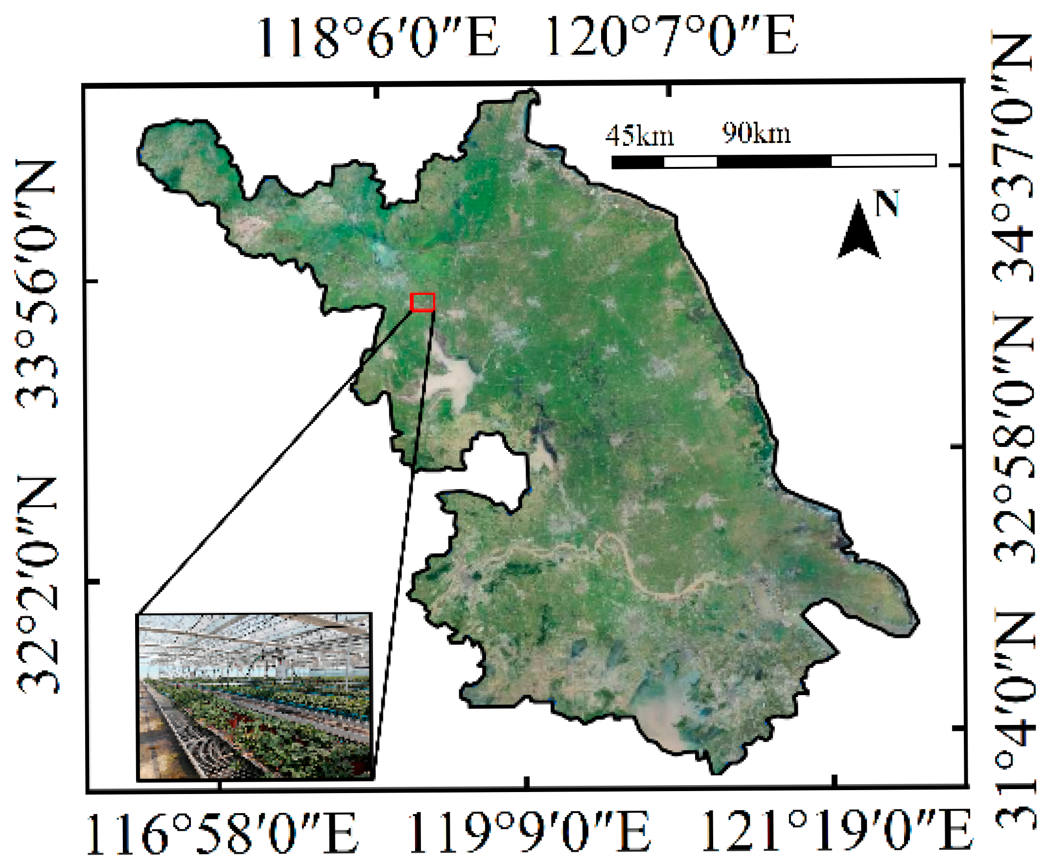
2.1. Experimental Materials

The salt stress experiment was conducted at Suqian Research Institute of Nanjing Agricultural University, Yanghe Town, Suqian City, Jiangsu Province, China (33°45′ N, 118°26′ E) from June to July 2024 (as shown in Figure 1). The average maximum and minimum temperatures at the experimental site in July were 32 and 24 °C, respectively. The experimental park covered an area of 52 mu, with 21 standardized multi-span greenhouses, a 50 m greenhouse, and a single span of 8 m.
Franti were used for seedling cultivation on the seedbed. The test soil was provided by Weifang Lurun Agricultural Technology Co., Ltd. (Weifang, China). The soil bulk density was 1.2 g/cm3, and the soil nutrient content (calculated based on the drying mechanism) was 0.68 g/L total nitrogen, 0.27 g/L phosphorus anhydride (P2O5), and 0.36 g/L potassium oxide (K2O). The diameter of the flowerpot, bottom diameter, and height were 15.6 cm, 11.0 cm, and 13.5 cm, respectively. Each pot was filled with 1 kg of soil. On 1 July 2024, healthy strawberry seedlings with seven fully expanded leaves were selected and transplanted into the flowerpots for planting, with one plant per pot, for a total of 100 plants. After the planting value was fixed, the seedlings were watered once and normal growth was maintained for 20 days. The management was conducted in accordance with the conventional management specifications of a local greenhouse.

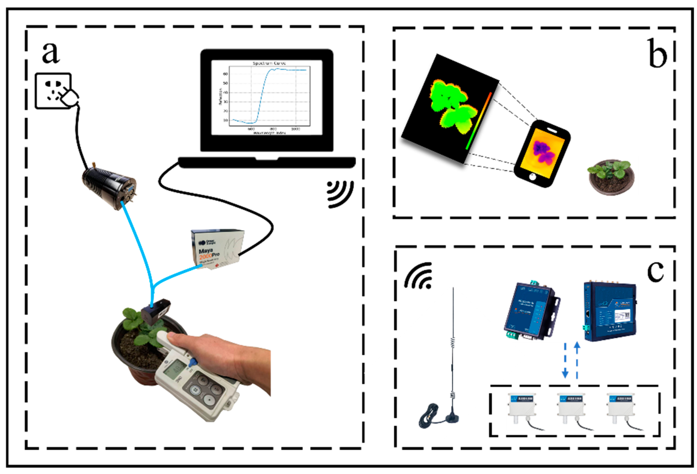
2.2. Experimental Equipment

The experiment utilized the following equipment:
Spectrometer: Ocean Optics Maya 2000Pro (Ocean Optics Inc., Orlando, FL, USA, 400–1000 nm range, 14 μm2 pixel size, 18 ms integration time);
Light source: Ocean Optics krypton-tungsten halogen (Ocean Optics Inc., Orlando, FL, USA, 360–2500 nm range);
SPAD instrument: SPAD-502 (Konica Minolta Inc., Tokyo, Japan) for measuring the chlorophyll content;
Temperature monitoring: Jinan UIoT system (USR IOT Tech. Ltd., Jinan, China, Lora wireless gateway, IO controller, and RS485 output temperature sensor);
Thermal infrared camera: FLIR ONE (Teledyne FLIR Inc., Wilsonville, OR, USA, 160 × 120 resolution, temperature range—20–400 °C).

2.3. Experimental Design

To enable the strawberry seedlings to adapt fully to the new cultivation environment, the experiment was started three weeks after the strawberry seedlings were planted. Four experimental groups were established for the salt stress experiment: S1 (0 mmol/L NaCl), S2 (50 mmol/L NaCl), S3 (100 mmol/L NaCl), and S4 (150 mmol/L NaCl). The experiment was conducted using a randomized block design with 25 samples for each treatment. For each sample, two leaves were selected and five data points were selected in the middle part of each leaf (avoiding the top, bottom, veins, and leaf edges) to collect the spectra as biological replicates.
The experiment was conducted from 8:00 to 18:00 daily, and five data points were collected for each young leaf every 3 min. Using the SPAD meter, the relative chlorophyll content was collected three times for each spectral point, and the results were averaged. Simultaneously, the FLIR ONE was used to obtain thermal infrared information from the leaves where the spectrum was collected, and the temperature region of interest (ROI) was extracted from the data points of the collected spectrum using FLIR TOOL (v4.1) software. Because the subsequent modeling depended on the accuracy of the test data, the spectrum collection point, SPAD sampling point, and extracted temperature area of interest needed to be consistent during the experiment. In addition, to measure the ambient temperature, the temperature sampling interval of the human–cloud system was set to 3 min. After data collection, the data were uploaded to the cloud platform quickly, and the cloud data were downloaded locally after the experiment. The test process is illustrated in Figure 2.

2.4. Experimental Methods

2.4.1. Spectral Data Acquisition and Calibration

The spectrum acquisition system was mainly composed of a back-illuminated high-sensitivity spectrometer, halogen light source, Y-type optical fiber, refined alloy steel probe, and computer. The three ports of the Y-type optical fiber were correctly connected to the halogen light source, spectrometer, and refined alloy steel probe according to the identification position. The probe had a 45° inclined measurement hole and a 90° vertical measurement hole. All spectra measured in this test were obtained using the 90° measurement hole. When the alloy steel probe was used vertically, it lightly touched the blade (not pressed).
After the test started, the spectrum acquisition device was connected as shown in the Figure 3, the halogen light source was preheated for 20 min, the knob on the halogen light source was adjusted to make the light source stable, Ocean View (v2.0) software was opened simultaneously, and the “Reflection Spectrum Measurement” mode was selected according to the settings. At this time, the halogen light source remained on, and the integration time was set to 12–20 μm according to the light intensity during measurement. According to the usage requirements, the bright spectrum only needed to exceed 80% of the maximum spectrum. The steel probe lightly touched the diffuse reflectance standard white board (PTFE material, Ocean Optics, Inc., Orlando, FL, USA), and the spectrum curve (bright spectrum) was saved. The spectrum was then turned off, the steel probe was lightly touched on the diffuse reflectance standard white board again, and the spectrum curve (dark spectrum, also called dark noise) was saved. The halogen light source was turned on again to correct the spectral curve, as shown in Figure 3.

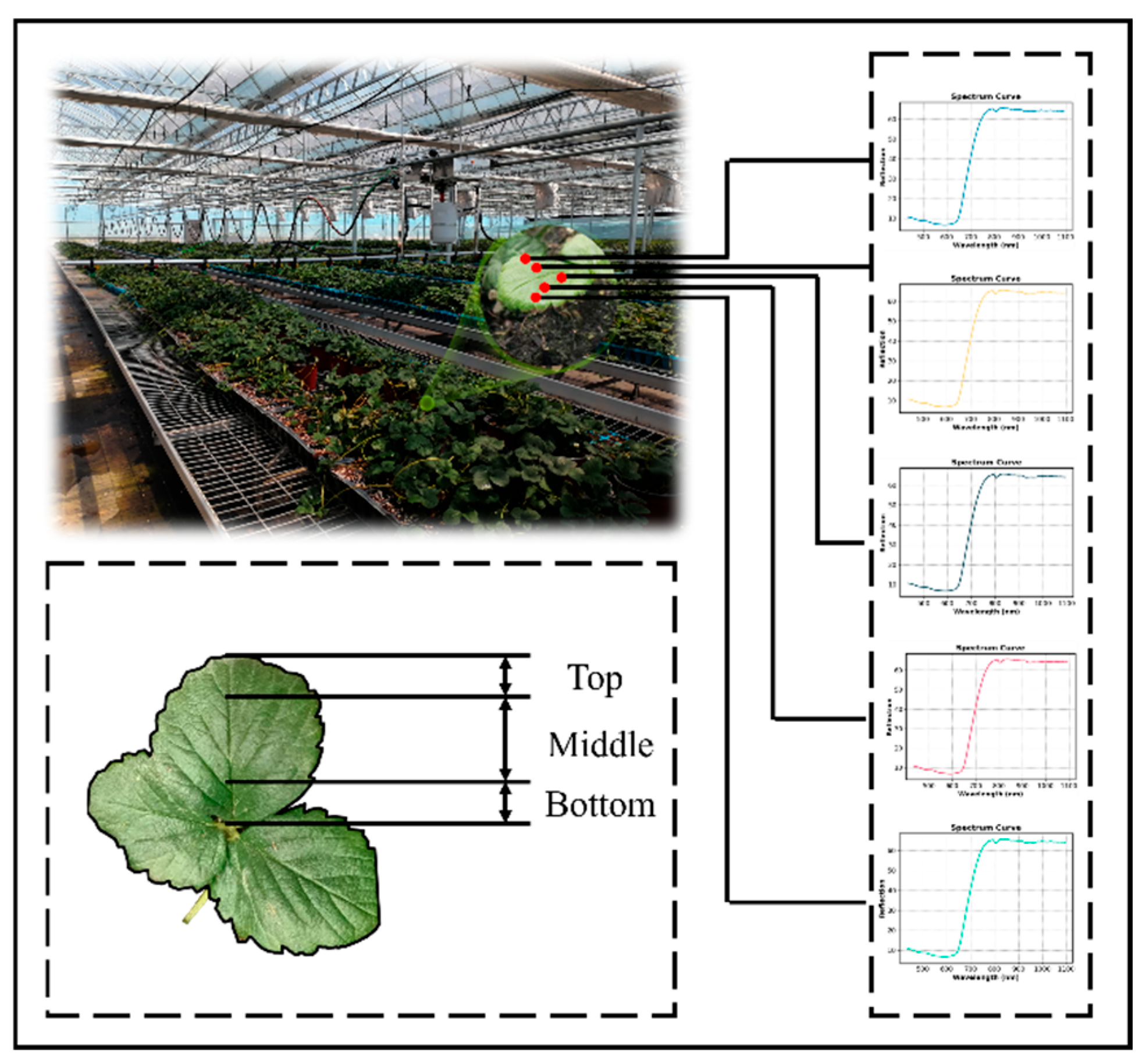
2.4.2. Spectral Data Extraction

Complete, healthy, and fully expanded strawberry leaves were selected for spectrum collection. The sampling data were primarily obtained in the middle of the leaves, avoiding the veins and edges. Five regions of interest were selected in each strawberry leaf for spectral data collection. The five spectral data points were then averaged using a script program, and the results were utilized as the sample data for the subsequent processing, as shown in Figure 4.

2.4.3. Relative Chlorophyll Content Collection

The relative chlorophyll content collection was synchronized with the spectral data, mainly relying on the SPAD-502 instrument. After the device was switched on, it was pressed for 2 s. When the machine made a “beep” sound, the measuring head was released to complete the self-test and spectral calibration of the machine. The leaf area was then clamped for collection in the leaf clamp of the SPAD instrument, pressed for 2 s and released, and the data were read. Each data point was sampled three times, and the results were averaged and recorded. Fifteen SPAD values were collected for each leaf and averaged to determine the relative chlorophyll content.

2.4.4. Leaf Temperature Extraction and Canopy Temperature Visualization

The high thermal resolution and universal interface of the FLIR ONE camera significantly improved the convenience of obtaining thermal imaging images. When using this device, we only needed to connect the interface of the FLIR ONE camera to the Type C female port of a mobile phone and use the FLIR APP to complete the acquisition of thermal imaging images. The leaf temperature was extracted from the same ROI as the relative chlorophyll content and spectral data. The temperature extraction process involved importing the captured thermal infrared image into FLIR Tool software and selecting a rectangular ROI with a size of 5 × 5 pixels to calculate the average temperature of the pixels in the boxed area.
Temperature visualization involved visualizing the canopy temperature of strawberry seedlings under salt stress, as shown in Figure 5. For a thermal infrared image, FLIR TOOL software was used to separate the RGB image and the temperature data file of the same size as the image. Each point in the temperature data file represented the temperature of a pixel, with a total of 19,200 thermal pixels (160 × 120 pixels). The separated RGB image and temperature data files were processed separately. For the RGB image, the strawberry leaf canopy mask was produced using color-space transformation, and denoising. The temperature data were normalized and the strawberry canopy mask was then nested in the preprocessed temperature data to obtain a grayscale temperature image. Finally, the display and dynamic changes in the canopy of strawberry seedlings under stress were realized using a pseudo-color display.
Because temperature measurement considerably depended on the measurement accuracy of the sensor, the accuracy of the temperature measurement is directly related to the accuracy of the subsequent modelling. The ROI selection, extraction of the ROI area temperature, and temperature visualization all depended on accurate temperature measurement. Therefore, in the laboratory, the canopy temperature measured and calculated using FLIR ONE was first calibrated. Specifically, five standard, thin steel sheets were placed in a climate chamber, and the temperature of the climate chamber was set at 40 °C for 20 min. The standard steel sheets were then taken out and left to cool at room temperature (16 °C). Thermal infrared images of the standard steel sheets were continuously collected at a sampling interval of 20 s for 8 min. In FLIR TOOL software, the square ROI tool was used to select the area and calculate its average temperature. Simultaneously, the segmentation algorithm mentioned in the temperature visualization process was used to segment the steel sheets and extract the temperature to verify the accuracy of the temperature fusion algorithm in calculating the canopy temperature.

2.5. Data Analysis

2.5.1. Spectral Data Preprocessing

The sorted spectral data were first preprocessed to eliminate noise and scattering effects and to highlight the effective information of the sample. Preprocessing can improve the quality of the spectral data and provide a more accurate benchmark for subsequent modelling and analysis. Common preprocessing methods include convolution smoothing, maximum–minimum normalization, standard normal correction (SNV), and multivariate scatter correction (MSC). For the preprocessed spectral data, the signal smoothness, signal-to-noise ratio, and correlation coefficient were compared to select the combination of preprocessing methods with the best effect.
S m o o t h n e s s = S t d ( d 2 I d λ 2 )
S N R = m e a n   ( S p e c t r u m ) s t d   ( n o i s e )
r i j = k = 1 m ( x i k x i ¯ ) ( x j k x j ¯ ) k = 1 m ( x i k x i ¯ ) 2 k = 1 m ( x j k x j ¯ ) 2
where, in (1), I is the spectral intensity, λ is the wavelength, d 2 I d λ 2 is the second-order derivative of the spectral curve, and Std is the standard deviation of the second-order derivative; in (2), mean (Spectrum) is the average intensity of the spectral signal, and std (noise) is the standard deviation of the noise; in (3), m is the number of wavelengths, x i k is the spectral intensity of sample i at wavelength k, x i ¯ is the average intensity of sample i at all wavelengths, x j k is the spectral intensity of sample j at wavelength k, and x j ¯ the average intensity of sample j at all wavelengths.
The signal smoothness was used to determine the smoothness stability of the signal by calculating the standard deviation of the second-order derivative of the spectral curve. The value range was [0, ∞). The smaller the value, the smoother the signal. The signal-to-noise ratio (SNR) was calculated as the average ratio of the signal to noise. The larger the value, the better. The correlation coefficient was that between each wavelength and the target value and had a value range of [–1, 1]. The closer the correlation coefficient to the either end, the better.

2.5.2. Wavelength Screening Method

In high-dimensional spectral data, important information about crops is often hidden due to the massive amount of data. To optimize the spectral features, screening the key wavelengths that best represent crop information has become the preferred strategy for researchers in the field of spectral analysis. In this study, we combined three common wavelength selection algorithms, Continuous Projection Algorithm (SPA), Competitive Adaptive Reweighting Algorithm (CARS), and Variable Importance Projection Algorithm (VIP), and selected representative wavelengths with reference to other studies, ultimately obtaining the spectral bands that best reflected the characteristics of leaf nutritional changes.

2.5.3. Model Establishment and Evaluation

In this study, two types of spectral models were established to predict and analyze the samples. The models of the first type utilized traditional machine learning methods, including the partial least-squares regression (PLSR), random forest, support vector regression (SVR), kernel ridge, K-nearest neighbor, and decision tree models. These models extract features from the spectral data for regression analysis. The models of the second type were one-dimensional (1D) convolutional neural network (1D-CNN) models based on deep learning. This type of model can automatically learn complex nonlinear features from spectral data. The traditional machine learning and 1D-CNN models simultaneously integrated the temperature information, thereby enhancing the interpretability and predictive ability of the spectral model. In this study, the prediction performance of the traditional spectral model was evaluated using the coefficient of determination (R2), root mean square error (RMSE), and relative percent difference (RPD), and the deep learning model was evaluated using the RMSE and mean absolute error (MAE). R2 was used to measure the linear correlation between model predictions and actual values. The closer the value is to 1, the better the model fits. The RMSE indicates the average error in the model prediction. The smaller the value, the higher the accuracy. The RPD can be used to measure the reliability of a model. An RPD value of less than 1.4 indicates that the model prediction ability is poor, 1.4–2.0 indicates that the model prediction is reliable, and greater than 2.0 indicates that the model prediction performance is excellent. The MAE is used as a measure of the difference between the predicted and true values in deep learning.
R 2 = 1 i = 1 n ( y i y i ^ ) 2 i = 1 n ( y i y ¯ ) 2
R M S E = 1 n i = 1 n ( y i y i ^ ) 2
R P D = 1 n i = 1 n ( y i y ¯ ) 2 R M S E
M A E = 1 n i = 1 n y i y i ^
In these formulas, y i , y i ^ , y ¯ , and n denote the i-th actual value, i-th predicted value, average of the actual values, and number of samples, respectively.
The data represent the arithmetic mean after three repetitions. SPSS27 was used for analysis of variance and Duncan’s multiple comparisons. Python3.9 was utilized for temperature visualization and model building. The PyTorch (v2.0.0) framework was used for deep learning. The computing platform CPU used was Intel i5-12400F, with 32.0 GB, and the GPU used was Nvidia 3060Ti. Origin was used for graphical drawing.

3. Results

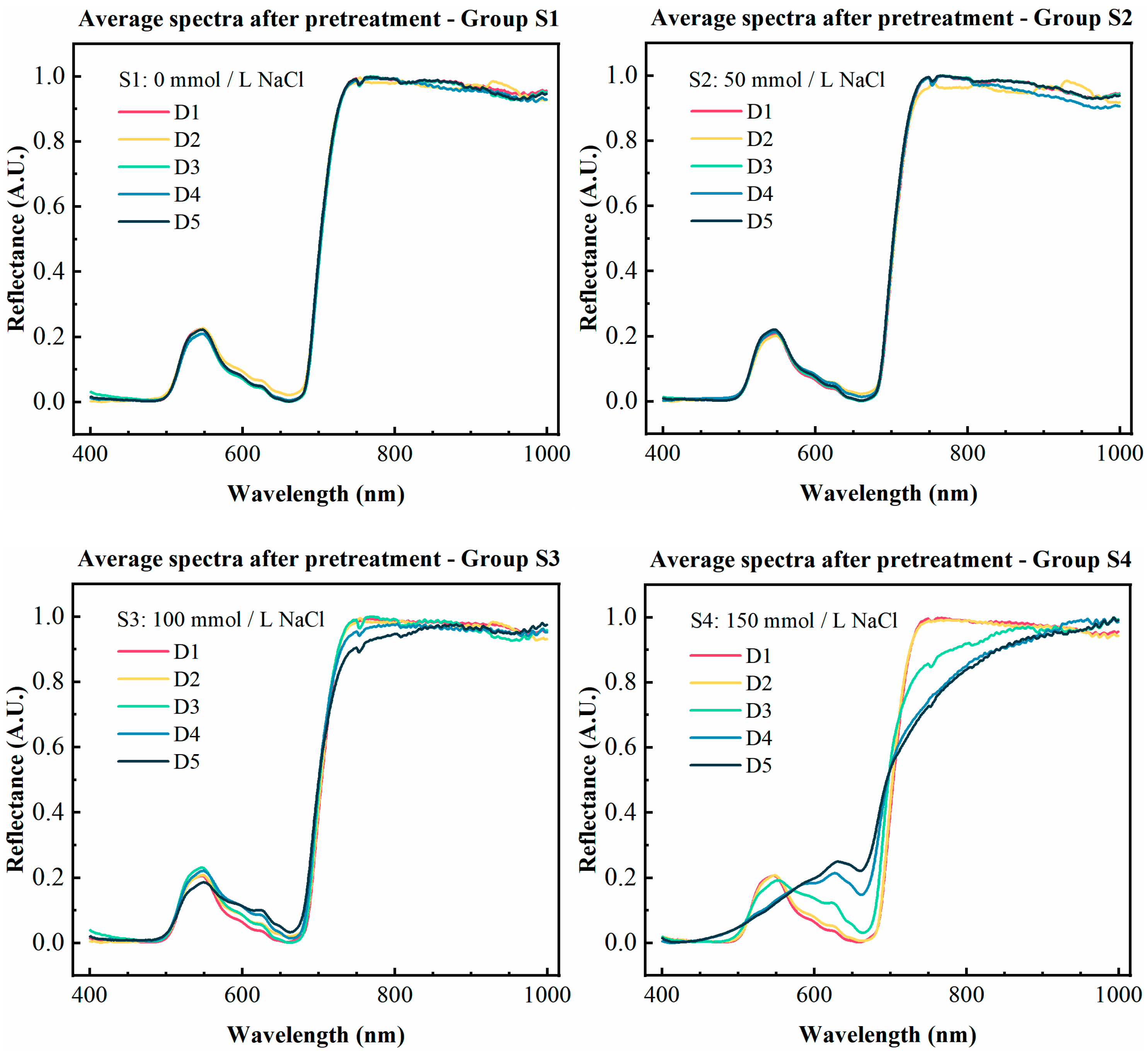
3.1. Spectral Preprocessing

Convolution smoothing and maximum–minimum normalization are essential basic steps in spectral data processing. The various preprocessing methods mentioned in this paper are based on convolution smoothing and normalization. Therefore, the differences between the methods in the subsequent steps were compared. Five preprocessing methods were used: (1) smoothing-normalization, (2) smoothing-normalization-SNV, (3) smoothing-normalization-MSC, (4) smoothing-normalization-MSC-SNV, and (5) smoothing-normalization-SNV-MSC. The results are summarized in Table 1.
The results indicate that using the SNV and processing methods in the preprocessing of the spectrum under salt stress increases the smoothness by an order of magnitude and reduces the SNR. Although the SNV can effectively deal with scattering interference, in practical applications, the sensitivity of the SNV to small noise introduces noise, increasing the SNR of the spectrum and decreasing the smoothness. In this study, only the smooth-normalized-MSC preprocessing method was used. Figure 6 shows the average spectra obtained after smooth-normalized-MSC preprocessing.
From the third day of the experiment, the spectral curves of salt stress treatment groups S3 and S4, especially the high-salt-concentration treatment group (S4), showed significant differences, which significantly impacted the physiological state of the strawberry seedlings. The spectral changes in the 600–900 nm band were particularly significant and mainly reflected the dual effects of salt stress on the plant chlorophyll and water dynamics. The red-light absorption peak at 650–680 nm gradually becomes passivated, which is mainly attributed to the decrease in chlorophyll content, and the spectral curves show upward trends in this band.
In addition, the red-edge region at 700–750 nm changes significantly, and the chlorophyll reflection peak shows a significant downward shift. This is because the degradation of chlorophyll weakens the red-edge displacement, which further reflects the deterioration in plant health. Simultaneously, salt stress considerably impacts the spectral characteristics in the near-infrared region (750–900 nm). The near-infrared reflection “platform area” of the strawberry seedlings almost completely disappears, indicating that salt stress affects not only the optical properties of chlorophyll but also the leaf tissue structure and the water reflection ability of the intercellular space.

3.2. Spectral Wavelength Screening

Spectral wavelength screening is an important method for reducing data dimension and discarding redundant information. Some differences existed between the different experimental scenarios. However, as the red-edge absorption peak (650–680 nm) and red-edge region (700–750 nm) are the most sensitive to changes in chlorophyll content, they are the most widely used in research related to plant physiological changes [46]. The wavelengths screened using the different methods in this study are listed in Table 2.
The SPA and CARS each screened out 10 characteristic bands, whereas the VIP algorithm screened out two continuous bands located in the red-edge region (700–750 nm) and the near-infrared key segment (760–900 nm). In this study, to optimize the spectral characteristics further and avoid the limitations of using a single method, the three screened bands were comprehensively analyzed and combined with the summary by Sanaeifar et al. [47] of characteristic wavelengths in plant salt stress; the characteristic bands with higher representativeness in each method were selected, and a new characteristic wavelength set was reconstructed [48]. The characteristic wavelengths finally selected were [564.08, 673.17, 699.59, 738.63, 753.23, 824.93, and 930.50], corresponding to seven characteristic bands.

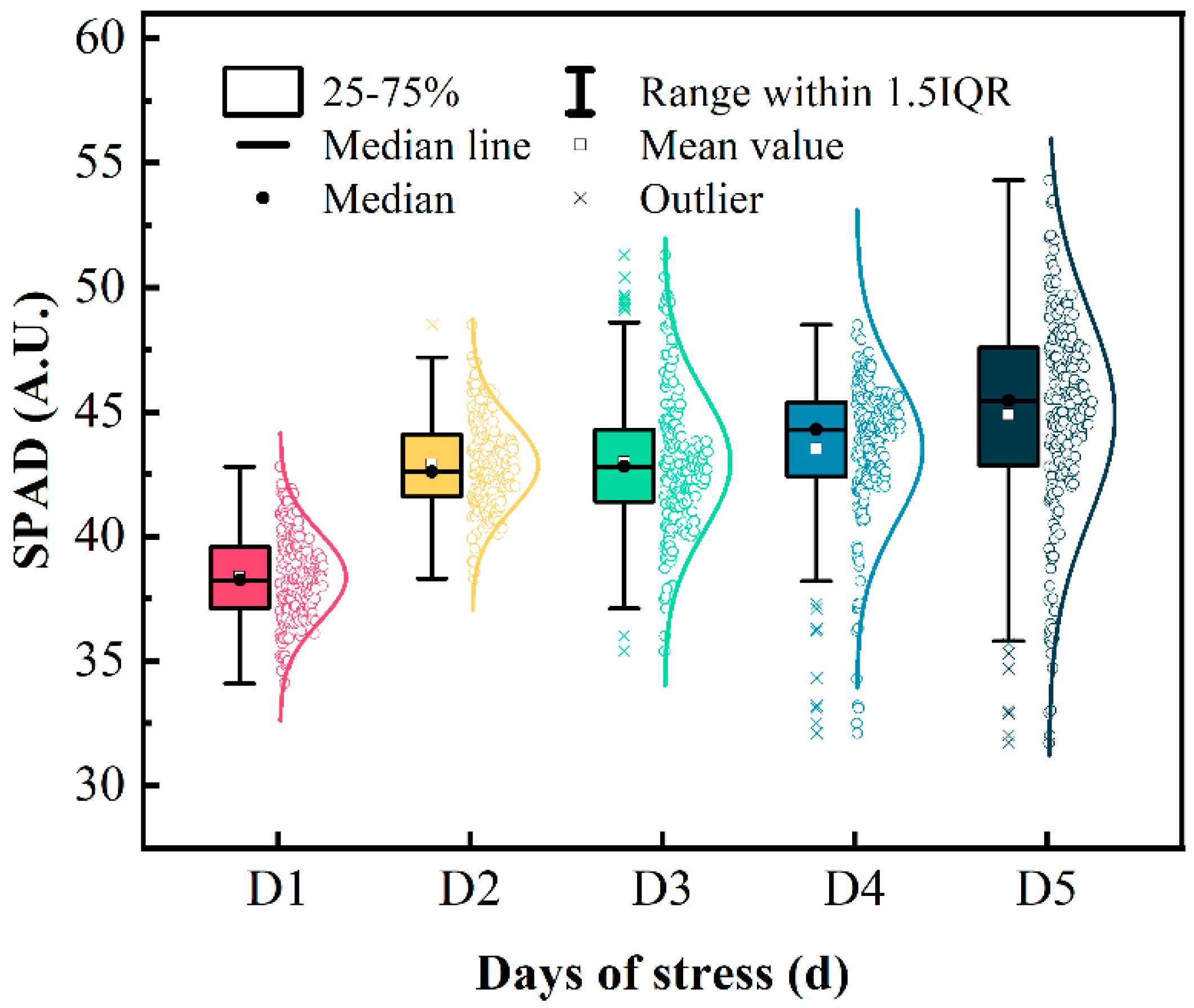
3.3. Relative Chlorophyll Content

Although overlaps were observed among certain treatments (e.g., S1 and S2; S1 and S3), the overall variation in the SPAD values still demonstrated a clear response to increasing salinity levels. In particular, a significant reduction in the SPAD was detected under the highest salt concentration (S4), a result that differed markedly from those obtained using the lower treatments. These findings suggested that, despite partial overlaps, the applied salinity gradient effectively induced physiological differences in the seedings (Table 3).
As a dimensionless parameter, the relative chlorophyll content SPAD has a wide range of applications in agronomic crop phenotyping. By statistically analyzing SPAD data, we can gain an in-depth understanding of the inherent structure of the data, select appropriate methods for subsequent modelling, and analyze emerging patterns to achieve a high degree of integration of crop phenotypic information. Figure 7 shows the distribution of and changes in the SPAD data during the experimental period.
Two basic observations can be made from Figure 7:
(1) The overall distribution is normal; however, the σ value of the SPAD is smaller in the early stage, indicating that the data are more concentrated. In the later stage, as the chlorophyll is severely damaged and the leaves become inactive, the SPAD concentration worsens, and the corresponding probability density curve is flatter.
(2) From the third day of salt stress exposure, the number of abnormal points exceeding 1.5 IQR in the SPAD data increased, which was closely related to chlorophyll destruction. In particular, on D5, the interquartile range of the box is higher than those of the other experimental groups, indicating that the relative chlorophyll content was considerably affected in the later period.

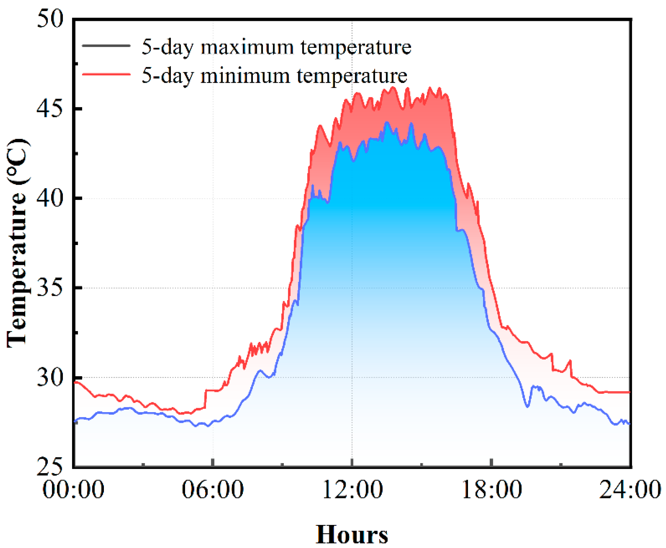
3.4. Visualization of Environmental Temperature Changes and Canopy Temperature

An increasing degree of salt stress leads to abnormal leaf temperatures. Simultaneously, the environmental temperature indirectly affects the leaves, thus affecting the physiological state of seedling leaves. The environmental monitoring temperatures are shown in Figure 8. From 8:00 to 18:00 daily, the average environmental temperature reached 38.84 °C, and the highest temperature occurred between 13:30 and 14:00 daily.
Dynamic changes in strawberry leaf temperature indirectly reflect the adaptability of seedlings to salt stress. As shown in Figure 9, the temperature of the main stem of the seedlings is higher than that of the leaves, whereas for a single leaf, the temperature at the petiole is the highest and gradually decreases in a diffuse manner along the main vein. The average canopy temperatures in groups S1 and S2 did not change significantly. During the stress period, the average canopy temperature increased by 0.2 °C and 0.6 °C in groups S1 and S2, respectively. The leaf temperature in S2 increased slightly only after D4. In contrast, for groups S3 and S4, as the salt stress worsened, the leaf temperature increased significantly. During the stress period, the average canopy temperature increased by 2.5 °C and 3.1 °C for groups S3 and S4, respectively. The accumulation of stress time further aggravated the effect of temperature increase. The average canopy temperature of S4 reached a maximum of 30.9 °C in D5.

3.5. Establishment of Spectrum-Relative Chlorophyll Content Model

3.5.1. Classical Machine Learning Method

The five classic machine learning methods are compared using the R2, RMSE, and RPD indicators in Table 4. For R2, a commonly used indicator in classic machine learning methods, the best model is the decision tree model processed by S1, and the R2 and the RPD are optimal in all models in this case. The best R2 value of the remaining three models appears in S1. Even for the PLSR model, the R2 index of S3 is only slightly higher than that of S1 (0.005), indicating that, for most experimental treatment groups, the increase in stress time decreases the accuracy of the model prediction results, showing a certain nonlinear response. Among all the models, the random frost model has the worst R2 performance under the four salt stress treatments, which could be owing to the complexity of the model.
When the five classic machine learning models are integrated with the ambient temperature (Table 5), the performance of R2 varies. However, only the performance of the Kernel Ridge model under different stress treatments is improved, indicating that Kernel Ridge can reflect the changes in ambient temperature during salt stress, particularly in S3, where the improvement rate in the R2 reaches 8.59%. When the five classic machine learning models are integrated with the leaf temperature (Table 6), the R2 values of 80% of the models are improved. The decision tree performs the best in the S3 process, with the greatest improvement in the R2 (32.3%). Simultaneously, for all experimental treatments, integrating fusion models PLSR and Kernel Ridge with the leaf temperature improves the R2 values of the models to varying degrees, extracts relevant features from the leaf temperature, and improves the prediction ability of the models.

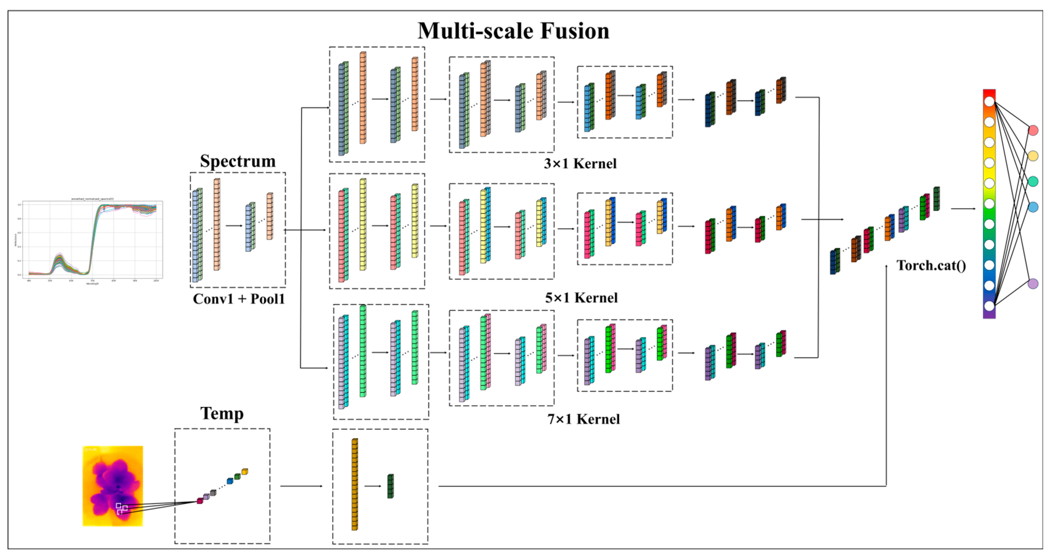
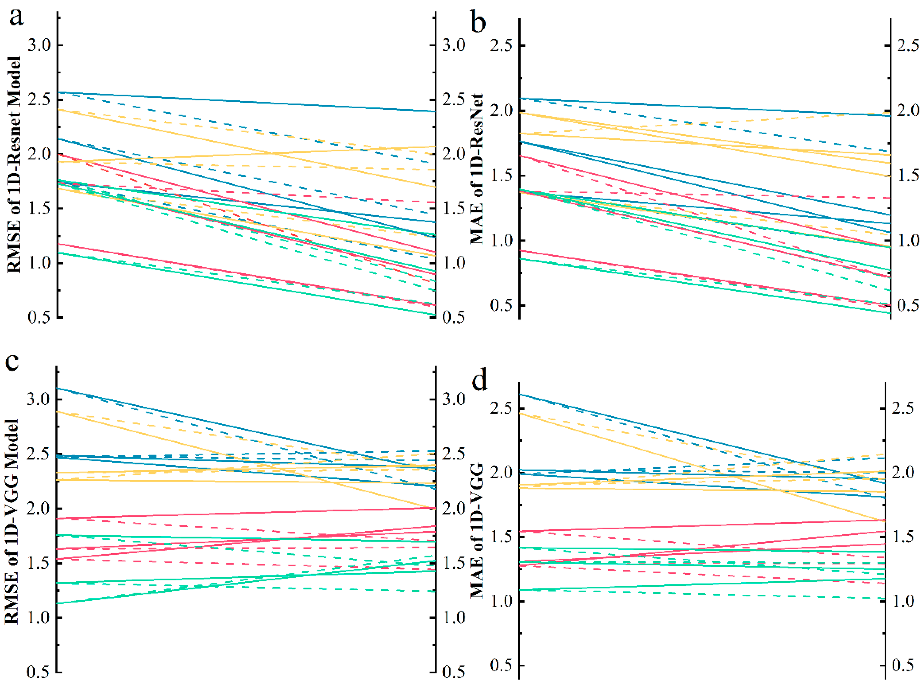
3.5.2. Building a Deep Learning Model

Three deep learning models were used to model directly the relationship between the model without preprocessing (normalization, MSC) and the relative chlorophyll content. The ambient and leaf temperatures were integrated to build the model. Because traditional CNN, ResNet, and VGG models are mainly for two-dimensional image data, feature extraction is determined by an n × n convolution kernel. During the extraction of 1D spectral data, the convolution kernel was set to n × 1 to improve the ability of the convolution kernel to extract spectral features. Figure 10 shows the process of the parallel extraction of spectral features using a 1D neural network.
As shown in Table 7, for the three deep learning network models, the 1D-ResNet model proposed based on the ResNet infrastructure has the best RMSE, and both the 1D-ResNet models integrating the ambient and leaf temperature can reduce the RMSE and MAE to varying degrees. Although the 1D-MSCNN and 1D-VGGNet models under most experimental treatments and the deep learning models that integrate temperature (ambient temperature or leaf temperature) can also improve the model’s prediction ability, the models similar to the 1D-VGGNet model when integrating the ambient temperature in S3 and S4 (1D-VGGNet + AT (S3) and 1D-VGGNet + AT (S4)) occasionally have higher RMSEs and MAEs for the prediction results than the 1D-VGGNet model (1D-VGGNet (S3) and 1D-VGGNet (S4)).
For both the 1D-MSCNN and 1D-VGGNet models, the integration of leaf temperature can effectively improve the prediction ability of the models. However, in the other models, the introduction of ambient temperature sometimes acts as noise, thereby reducing the RMSE and MAE. For example, the RMSE of the 1D-MSCNN + AT (S1) model under S1 treatment is 5.29% lower than that of 1D-MSCNN (S1), whereas the MAE of the 1D-VGGNet-AT (S3) model under the S3 treatment is 10.94% lower than that of 1D-VGGNet (S3).

4. Discussion

4.1. Comparison of Preprocessing Methods

After completing the smoothing–normalization preprocessing of the spectrum, the MSC and SNV preprocessing methods and their combinations were used. In particular, for a combination of the two methods, the order of the two algorithms directly affect the quality of the final spectral data [49,50]. The MSC algorithm is primarily used to correct the scattering effect of the spectrum and reduce the spectral changes caused by factors such as particle size and surface characteristics. The SNV algorithm was further normalized to reduce the baseline drift. The MSC-SNV algorithm sequence can first remove the scattering effect and then perform normalization. However, if the SNV-MSC algorithm sequence is used, the overall structure of the data changes, and noise and potentially useful information are eliminated. In this experiment, we tested the application of the SNV algorithm after MSC, which resulted in a sharp decrease in the SNR from 18.76 to 1.66. This drop was attributed to the nature of SNV, which standardizes each spectrum by removing its mean and scaling by its standard deviation, thereby reducing the overall signal amplitude relative to noise. Therefore, only the MSC algorithm module was used after smoothing–normalization preprocessing, and the SNV algorithm was not introduced.

4.2. Temperature Trend

Salt stress reduces the water absorption capacity of strawberries, causing stomatal closure and reduced transpiration, which increase the leaf temperature, affecting the photosynthetic efficiency and physiological functions of strawberries [51,52]. A similar trend was observed in the SPAD values under varying the salinity treatment, supporting the notion that salt stress adversely affects chlorophyll content, as also reported by Chen and Taibi [53,54]. Strawberries are low-growing creeping crops and their stolons play an important role in the growth process. During the collection of leaf temperature, ground radiation heat seriously affects the temperature of the stems because the height of strawberry stems from the ground does not exceed 10 cm in the early growth stage. Therefore, at all stages of stress, the temperature of the strawberry stems is high, and the temperature is the highest is near the central growth point. This is similar to the previous tomato canopy temperature monitoring results obtained by Yang et al. [55]; however, a tomato plant is tall and grows upright, and the impact of ground heat radiation on leaf temperature is mainly limited to old, bottom leaves. In contrast, the higher temperature observed in the central region of the strawberry leaves can be attributed to the fact that these leaves are not fully expanded. In this early developmental stage, the smaller surface area of the leaves leads to a greater tendency for heat accumulation due to limited airflow and reduced convective cooling. Once the leaves fully expand, the increased surface area facilitates better heat dissipation through enhanced interaction with the surrounding air, resulting in temperatures lower than those of the central, undeveloped leaves.
The leaves of strawberry seedlings gradually expand from the growth point, and the transport of nutrients and water also expands along the main veins to the surrounding areas. Therefore, heat is also expressed as expanding from the stem and petiole to the edge of the leaf. This temperature distribution reflects the unique thermal regulation mechanism of strawberry leaves during growth, particularly in the process of water and nutrient transport. The main veins typically accumulate more heat, whereas the peripheral region maintains a lower temperature due to its enhanced heat dissipation capacity. The edges of the strawberry leaves are irregularly serrated and fluffy. These features are conducive to improving the heat-dissipation capacity. Therefore, even in D4 and D5, when the stress was more severe (S4), the water transport in the strawberry body was obstructed somewhat; however, the temperature of the leaf near the outer edge of the leaf was still low [56,57,58].

4.3. Model Comparison

The application of classic machine learning models effectively builds a bridge between the spectra and relative chlorophyll content; is widely used in various plant studies, specifically in phenotypic studies of aspects such as the plant nitrogen and relative chlorophyll content; and can achieve relatively good results [59,60]. Owing to the high-dimensional characteristics of spectral data, complex data preprocessing is required to remove redundant information before constructing a spectrum-relative chlorophyll content model under salt stress conditions, which poses a challenge to automated phenotypic monitoring.
The predictive performance of the proposed spectral–temperature fusion model was consistent with the physiological trends observed under varying salt stress levels. Specifically, the performance metrics of the predictive model under low salinity conditions (S1, S2) were generally superior to those under high salinity levels (S3, S4). This difference may be attributed to several factors: Under low salt conditions, plants may exhibit more consistent physiological responses, enabling the model to capture the underlying patterns more accurately. In contrast, under high salt stress, the physiological responses of plants become more complex, involving a range of stress-induced processes such as ion toxicity and osmotic changes, which may increase the variability in the data and make accurately predicting the plant status more difficult. However, to enhance the physiological relevance of the model further, future studies could incorporate additional direct physiological and biochemical indicators, such as stomatal conductance, net photosynthesis, plant biomass, and other stress-related markers. These parameters could provide a more comprehensive understanding of how plants respond to salt stress, thus enabling the development of even more accurate and biologically grounded predictive models. Integrating these physiological metrics with spectral data could also help refine the model predictions and offer deeper insights into the underlying mechanisms of plant stress tolerance.
In the process of spectral modeling, deep learning approaches bypass traditional steps such as preprocessing and wavelength selection, which enhances the computational efficiency. However, this also introduces the challenge of dimensionality explosion, which necessitates careful handling of model complexity and feature selection. Based on the RMSE, 1D-ResNet achieved performance similar to that of the classic machine learning model. This is mainly attributed to the introduction of a residual module. The residual module effectively alleviates the gradient vanishing problem in the deep network by introducing jump connections and can better extract and capture important information from the data [61]. Although the multi-scale 1D-CNN model reduces the time cost of the model by parallel calculation of multiple convolution kernels, the residual module in 1D-ResNet constructs a “shortcut path” to allow information to bypass some layers, thereby avoiding problems such as overfitting or gradient explosion in the deep network during training. Therefore, the 1D-ResNet model shows high robustness and prediction accuracy [62].
The leaf temperature not only directly reflects the ambient temperature but also integrates the physiological and biochemical responses of plants to salt stress. Deep learning models that incorporate the ambient temperature or leaf temperature add a temperature dimension to explain the inversion of stress on the spectrum and relative chlorophyll content. The ambient temperature mainly affects the leaves indirectly, whereas the leaf temperature directly reflects the thermal state of the leaves. Therefore, in classical machine learning or deep learning models, most models that incorporate the leaf temperature can provide more accurate prediction results [63,64].
Different versions of both the ResNet and VGG models are provided for selection according to different task requirements. This study was based on the ResNet18 and VGG11 frameworks, which we improved for the spectral inversion task. We introduced a 1D convolution kernel to extract spectral features more effectively. Simultaneously, we attempted to introduce the 1D convolution kernel into models such as ResNet34, ResNet50, VGG13, and VGG16, as shown in Figure 11. Convolutional neural networks were originally primarily used in image recognition tasks to extract features from image data with complex structures [65]. Unlike image data, which often involve intricate spatial relationships and high-dimensional structures, spectral data are typically more structured and less complex. This inherent difference in data complexity suggests that simpler models may be equally, if not more, effective for spectral prediction tasks. The findings of this suggest that more complex deep learning architectures do not inherently improve spectral prediction accuracy. Conversely, well-designed models can more effectively extract relevant features and offer greater predictive capability. Future research may focus on simplifying commonly used architectures to accommodate spectral characteristics more effectively, potentially leading to more efficient and interpretable models for large-scale spectral data analysis.

5. Conclusions

In this study, we investigated the impact of salt stress on strawberry seedling growth in summer facility agriculture using multiple models to invert spectral data to estimate the relative chlorophyll content. The integration of multi-modal data enhances the predictive accuracy of plant nutritional status and can be adapted for precision agriculture practices. Future perspectives involve expanding the scope of this technique to other crops, refining the models with more comprehensive environmental factors, and incorporating additional direct physiological and biochemical indicators. The main conclusions are as follows.
(1) The spectral curves of groups S3 and S4 showed significant differences from the third day, specifically in the high-salt-concentration treatment group (S4), which had a significant impact on the physiological state of the strawberry seedlings.
(2) During the temperature visualization process, the stem temperature was the highest, followed by the petiole temperature. In the leaves, the temperature gradually decreased from the main vein to the leaf edge. In groups S3 and S4, the leaf temperature increased significantly with increasing salt stress. During the stress period, the average canopy temperature increased by 2.5 °C and 3.1 °C in groups S3 and S4, respectively, and the accumulation of stress time further aggravated this temperature increase effect. In S4, the average canopy temperature reached a maximum of 30.9 °C in D5.
(3) The impact of the ambient temperature on the performance of traditional machine learning models varied; however, the performance of the traditional machine learning model that incorporated leaf temperature improved by more than 80%. Among the deep learning models, 1D-ResNet18 + LT performed the best, with the RMSEs of groups S1, S2, S3, and S4 being 0.600, 0.625, 1.035, and 1.236, respectively, and the MAEs being 0.485, 0.511, 0.948, and 1.045, respectively. Future research may focus on simplifying commonly used architectures to accommodate spectral characteristics more effectively.

Author Contributions

Conceptualization, X.W. and H.Y.; methodology, X.Z.; software, Y.C.; validation, Y.S. and H.Y.; formal analysis, Z.W.; investigation, L.W.; resources, X.W.; data curation, W.L.; writing—original draft preparation, Y.S. and H.Y.; writing—review and editing, Y.S.; visualization, Z.W.; supervision, W.L.; project administration, X.W.; funding acquisition, X.W. All authors have read and agreed to the published version of the manuscript.

Funding

This research was funded by Jiangsu Province Modern Agricultural Machinery Equipment and Technology Promotion Project, grant number NJ2023-44 and Key technologies and Intelligent Equipment Research and Development for Efficient Production of Facility Strawberries, grant number CX(21)2006.

Data Availability Statement

The datasets used and/or analyzed during the current study are available from the corresponding author upon reasonable request.

Conflicts of Interest

The authors declare no conflicts of interest.

Abbreviations

The following abbreviations are used in this manuscript:
1D-CNNOne-dimensional convolutional neural network
ResNetResidual network
MSCNNMulti-scale convolutional neural network
IoTInternet of Things
MSCMultivariate scatter correction
SNVStandard normal correction
PLSRPartial least-squares regression
SVMSupport vector machine
SVRSupport vector regression
ATAmbient temperature
LTLeft temperature
R2Coefficient of determination
RMSERoot mean square error
RPDRelative percent difference
MAEMean absolute error
SNRSignal-to-noise ratio

References

  1. Food and Agriculture Organization of the United Nations (FAO). FAOSTAT: Crops and Livestock Products. 2024. Available online: https://www.fao.org/faostat/en/#data/QCL (accessed on 10 April 2025).
  2. IndexBox. World-Strawberries-Market Analysis, Forecast, Size, Trends and Insights Please mention the Source. Available online: https://www.indexbox.io/blog/strawberry-world-market-overview-2024 (accessed on 25 January 2025).
  3. Peng, Y.; Zhao, S.Y.; Liu, J.Z. Fused-Deep-Features Based Grape Leaf Disease Diagnosis. Agronomy 2021, 11, 2234. [Google Scholar] [CrossRef]
  4. Zhao, S.Y.; Peng, Y.; Liu, J.Z.; Wu, S. Tomato Leaf Disease Diagnosis Based on Improved Convolution Neural Network by Attention Module. Agriculture 2021, 11, 651. [Google Scholar] [CrossRef]
  5. Francisco, A.R.; Rosario, B.P.; Juan, M.B.; José, L.C. The Strawberry Plant Defense Mechanism: A Molecular Review. Plant Cell Physiol. 2021, 52, 1873–1903. [Google Scholar] [CrossRef]
  6. Coatsworth, P.; Gonzalez-Macia, L.; Collins, A.S.P.; Bozkurt, T.; Güder, F. Continuous monitoring of chemical signals in plants under stress. Nat. Rev. Chem. 2023, 7, 7–25. [Google Scholar] [CrossRef]
  7. Guo, J.; Yang, Z.; Karkee, M.; Jiang, Q.; Feng, X.P.; He, Y. Technology progress in mechanical harvest of fresh market strawberries. Comput. Electron. Agric. 2024, 226, 109468. [Google Scholar] [CrossRef]
  8. Singh, T.; Rajan, R.; Vamsi, T.; Kumar, A.; Ramprasad, R.R.; Gopichand, G.B.; Chundurwar, K. A Review on the Impact of Organic and Biofertilizer Amendments on Growth, Yield, and Quality of Strawberry. Int. J. Plant Soil Sci. 2023, 35, 147–158. [Google Scholar] [CrossRef]
  9. Wang, R.Y.; Yang, X.J.; Chi, Y.W.; Zhang, X.; Ma, X.Z.; Zhang, D.; Zhao, T.; Ren, Y.F.; Yang, H.Y.; Ding, W.J.; et al. Regulation of hydrogen rich water on strawberry seedlings and root endophytic bacteria under salt stress. Front Plant Sci. 2024, 15, 1497362. [Google Scholar] [CrossRef]
  10. Katel, S.; Mandal, H.R.; Kattel, S.; Yadav, S.P.S.; Lamshal, B.S. Impacts of plant growth regulators in strawberry plant: A review. Heliyon 2022, 8, e11959. [Google Scholar] [CrossRef]
  11. Lu, C.X.; Li, L.Y.; Liu, X.L.; Chen, M.; Wan, S.B.; Li, G.W. Salt stress inhibits photosynthesis and destroys chloroplast structure by downregulating chloroplast development-Related genes in Bobinia pseudoacacia Seedlings. Plants 2023, 12, 1283. [Google Scholar] [CrossRef]
  12. Turan, S.; Tripathy, B.C. Salt-stress induced modulation of chlorophyll biosynthesis during de-etiolation of rice seedlings. Physiol. Plant. 2014, 153, 477–491. [Google Scholar] [CrossRef]
  13. EI-Shal, R.M.; EI-Naggar, A.H.; EI-Beshbeshy, T.R.; Mahmoud, E.K.; EI-Kader, N.I.A.; Missaui, A.M.; Du, D.L.; Ghoneim, A.M.; EI-Sharkawy, M.S. Effect of nano-fertilizers on alfalfa plants grown under different salt stresses in hydroponic system. Agriculture 2022, 12, 1113. [Google Scholar] [CrossRef]
  14. Chen, Y.Y.; Wang, X.C.; Zhang, X.L.; Wang, D.Z.; Xu, X. A band selection method combining spectral color characteristics for estimating chlorophyll content of rice in different backgrounds. Spectrochim. Acta Part A. 2024, 24, 1386–1425. [Google Scholar] [CrossRef]
  15. Muhammad, A.; Zou, X.B.; Haroon, E.T.; Hu, X.T.; Allah, R.; Sajid, B.; Zhao, H. Near-infrared spectroscopy coupled chemometric algorithms for prediction of antioxidant activity of black goji berries (Lycium ruthenicum Murr.). Food Measure. 2018, 12, 2366–2376. [Google Scholar] [CrossRef]
  16. Fan, S.X.; Li, J.B.; Xia, Y.; Tian, X.; Guo, Z.M.; Huang, W.Q. Long-term evaluation of soluble solids content of apples with biological variability by using near-infrared spectroscopy and calibration transfer method. Postharvest Biol. Technol. 2019, 151, 79–87. [Google Scholar] [CrossRef]
  17. Ge, X.; Sun, J.; Lu, B.; Chen, Q.S.; Xun, W.; Jin, Y.T. Classification of oolong tea varieties based on hyperspectral imaging technology and BOSS-Light GBM model. J. Food Process. Eng. 2019, 42, e13289. [Google Scholar] [CrossRef]
  18. Sun, J.; Zhang, L.; Zhou, X.; Yao, K.S.; Tian, Y.; Nirere, A. A method of information fusion for identification of rice seed varieties based on hyperspectral imaging technology. J. Food Process. Eng. 2021, 44, e13797. [Google Scholar] [CrossRef]
  19. Elsayed, S.; EI-Hendawy, S.; Elsherbiny, O.; Okasha, A.M.; Elmetwalli, A.H.; Elwakeel, A.E.; Memon, M.S.; Ibrahim, M.E.M.; Ibrahim, H.H. Estimating Chlorophyll Content, Production, and Quality of Sugar Beet under Various Nitrogen Levels Using Machine Learning Models and Novel Spectral Indice. Agronomy 2023, 13, 2743. [Google Scholar] [CrossRef]
  20. Liu, C.H.; Yu, H.Y.; Liu, Y.C.; Zhang, L.; Li, D.; Zhang, J.H.; Li, X.K.; Sui, Y.Y. Prediction of Anthocyanin Content in Purple-Leaf Lettuce Based on Spectral Features and Optimized Extreme Learning Machine Algorithm. Agronomy 2024, 14, 2915. [Google Scholar] [CrossRef]
  21. Zhu, W.J.; Li, J.Y.; Li, L.; Wang, A.C.; Wei, X.H.; Mao, H.P. Nondestructive diagnostics of soluble sugar, total nitrogen and their ratio of tomato leaves in greenhouse by polarized spectra-hyperspectral data fusion. Int. J. Agric. Biol. Eng. 2020, 13, 189–197. [Google Scholar] [CrossRef]
  22. Zareef, M.; Arslan, M.; Hassan, M.M.; Ahmad, W.; Ali, S.; Li, H.H.; Yang, Q.O.; Wu, X.Y.; Hashim, M.M.; Chen, Q.S. Recent advances in assessing qualitative and quantitative aspects of cereals using nondestructive techniques: A review. Tends Food Sci. Technol. 2021, 116, 815–828. [Google Scholar] [CrossRef]
  23. Huang, Y.P.; Li, Z.A.; Bian, Z.C.; Jin, H.J.; Zheng, G.Q.; Hu, D.; Sun, Y.; Fan, C.L.; Xie, W.J.; Fang, H.M. Overview of Deep Learning and Nondestructive Detection Technology for Quality Assessment of Tomatoes. Foods 2025, 14, 286. [Google Scholar] [CrossRef]
  24. Xu, S.Z.; Xu, X.G.; Zhu, Q.Z.; Meng, Y.; Yang, G.J.; Feng, H.K.; Yang, M.; Zhu, Q.L.; Xue, H.Y.; Wang, B.B. Monitoring leaf nitrogen content in rice based on information fusion of multi-sensor imagery from UAV. Precis. Agric. 2023, 24, 2327–2349. [Google Scholar] [CrossRef]
  25. Wei, L.L.; Yang, H.S.; Niu, Y.X.; Zhang, Y.N.; Xu, L.Z.; Chai, X.Y. Wheat biomass, yield, and straw-grain ratio estimation from multi-temporal UAV-based RGB and multispectral images. Biosyst. Eng. 2023, 234, 187–205. [Google Scholar] [CrossRef]
  26. Yang, Z.Y.; Owen, T.A.; Cai, W.W.; Hasan, T. Miniaturization of optical spectrometers. Science 2021, 371, eabe0722. [Google Scholar] [CrossRef]
  27. Li, A.; Yao, C.H.; Xia, J.F.; Wang, H.J.; Cheng, Q.X.; Penty, R.; Fainman, Y.; Pan, S. Advances in cost-effective integrated spectrometers. Light Sci. Appl. 2022, 11, 174. [Google Scholar] [CrossRef]
  28. Yang, M.; Kim, T.Y.; Hwang, H.C.; Yi, S.K.; Kim, D.H. Development of a palm portable mass spectrometer. J. Am. Soc. Mass. Spectrom. 2008, 19, 1442–1448. [Google Scholar] [CrossRef]
  29. Ang, K.L.M.; Seng, J.K.P. Big Data and Machine Learning with Hyperspectral Information in Agriculture. IEEE Access. 2021, 9, 36699–36718. [Google Scholar] [CrossRef]
  30. Li, L.Q.; Xie, S.M.; Ning, J.M.; Chen, Q.S.; Zhang, Z.Z. Evaluating green tea quality based on multisensor data fusion combining hyperspectral imaging and olfactory visualization systems. J. Sci. Food Agric. 2019, 99, 1787–1794. [Google Scholar] [CrossRef]
  31. Guo, M.Q.; Wang, K.Q.; Lin, H.; Wang, L.; Cao, L.M.; Sui, J.X. Spectral data fusion in nondestructive detection of food products: Strategies, recent applications, and future perspectives. Compr. Rev. Food Sci. Food Saf. 2024, 23, e13301. [Google Scholar] [CrossRef]
  32. Dai, C.X.; Huang, X.Y.; Huang, D.M.; Lv, R.Q.; Sun, J.; Zhang, Z.C.; Ma, M.; Aheto, J.H. Detection of submerged fermentation of Tremella aurantialba using data fusion of electronic nose and tongue. J. Food Process. Eng. 2019, 43, e13002. [Google Scholar] [CrossRef]
  33. Ignat, T.; Shavit, Y.; Rachmilevitch, S.; Karnieli, A. Spectral monitoring of salinity stress in tomato plants. Biosyst. Eng. 2022, 217, 26–40. [Google Scholar] [CrossRef]
  34. Ma, X.X.; Zeng, X.Y.; Huang, Y.R.; Liu, S.H.; Yin, J.; Yang, G.F. Visualizing plant salt stress with a NaCl-responsive fluorescent probe. Nat. Protoc. 2024, 20, 902–933. [Google Scholar] [CrossRef]
  35. Zahir, S.A.D.M.; Omar, A.F.; Jamlos, M.F.; Azmi, M.A.M.; Muncan, J. A review of visible and near-infrared (Vis-NIR) spectroscopy application in plant stress detection. Sens. Actuators A 2022, 338, 113468. [Google Scholar] [CrossRef]
  36. Calzone, A.; Cotrozzi, L.; Lorenzini, G.; Nali, C.; Pellegrini, E. Hyperspectral Detection and Monitoring of Salt Stress in Pomegranate Cultivars. Agronomy 2021, 11, 1038. [Google Scholar] [CrossRef]
  37. Das, A.; Bhattacharya, B.K.; Setia, R.; Jayasree, G.; Das, B.S. A novel method for detecting soil salinity using AVIRIS-NG imaging spectroscopy and ensemble machine learning. ISPRS 2023, 200, 191–212. [Google Scholar] [CrossRef]
  38. Dinh, T.H.; Watanabe, K.; Takaragawa, H.; Nakabaru, M.; Kawamitsu, Y. Photosynthetic response and nitrogen use efficiency of sugarcane under drought stress conditions with different nitrogen application levels. Plant Prod. Sci. 2017, 20, 412–422. [Google Scholar] [CrossRef]
  39. Liu, F.H.; Wang, X.R.; Wang, B.; Xiao, F.; He, K.Q. Physiological response and drought resistance evaluation of Gleditsia sinensis seedings under drought-rehydration state. Nature 2023, 13, 19963. [Google Scholar] [CrossRef]
  40. Liu, B.; Asseng, S.; Wang, A.N.; Wang, S.H.; Tang, L.; Cao, W.X.; Zhu, Y.; Liu, L. L Modelling the effects of post-heading heat stress on biomass growth of winter wheat. Agric. For. Meteorol. 2017, 247, 476–490. [Google Scholar] [CrossRef]
  41. Kong, Y.; Masabni, J.; Niu, G. Temperature and Light Spectrum Differently Affect Growth, Morphology, and Leaf Mineral Content of Two Indoor-Grown Leafy Vegetables. Horticulturae 2023, 9, 331. [Google Scholar] [CrossRef]
  42. Santos, T.B.D.; Ribas, A.F.; Souza, S.G.H.; Budzinski, I.G.F.; Domingues, D.S. Physiological Responses to Drought, Salinity, and Heat Stress in Plants: A Review. Stress 2022, 2, 113–115. [Google Scholar] [CrossRef]
  43. Das, B.; Manohara, K.K.; Mahajan, G.R.; Sahoo, R.N. Spectroscopy Based Novel Spectral Indices, PCA– and PLSR–coupled Machine Learning Models for Salinity Stress Phenotyping of Rice. Spectrochim. Acta Part A. 2020, 229, 117983. [Google Scholar] [CrossRef]
  44. Blasch, E.; Pham, T.; Chong, C.Y.; Koch, W.; Leung, H.; Braines, D. Machine Learning/Artificial Intelligence for Sensor Data Fusion—Opportunities and Challenges. IEEE Access 2021, 26, 80–93. [Google Scholar] [CrossRef]
  45. Ahmad, U.; Nasirahmadi, A.; Hensel, O.; Marino, S. Technology and Data Fusion Methods to Enhance Site-Specific Crop Monitoring. Agronomy 2022, 12, 555. [Google Scholar] [CrossRef]
  46. Zhu, K.Y.; Sun, Z.G.; Zhao, F.H.; Yang, T.; Tian, Z.R.; Lai, J.B.; Zhu, W.X.; Long, B.J. Relating Hyperspectral Vegetation Indices with Soil Salinity at Different Depths for the Diagnosis of Winter Wheat Salt Stress. Remote Sens. 2021, 13, 250. [Google Scholar] [CrossRef]
  47. Sanaeifar, A.; Yang, C.; Guardia, M.D.L.; Zhang, W.K.; Li, X.L.; He, Y. Proximal hyperspectral sensing of abiotic stresses in plants. Sci. Total Environ. 2023, 861, 160652. [Google Scholar] [CrossRef]
  48. Wan, L.; Li, H.; Li, C.S.; Wang, A.C.; Yang, Y.H.; Wang, P. Hyperspectral Sensing of Plant Diseases: Principle and Methods. Agronomy 2022, 12, 1451. [Google Scholar] [CrossRef]
  49. Rinnan, A.; Berg, F.V.D.; Engelsen, S.B. Review of the most common pre-processing techniques for near-infrared spectra. TrAC. Trends Anal. Chem. 2009, 28, 1201–1222. [Google Scholar] [CrossRef]
  50. Jiao, Y.P.; Li, Z.C.; Chen, X.S.; Fei, S.M. Preprocessing methods for near-infrared spectrum calibration. J. Chem. 2020, 34, e3306. [Google Scholar] [CrossRef]
  51. Galli, V.; Messias, R.D.S.; Perin, E.C.; Borowski, J.M.; Bamberg, A.L.; Rombaldi, C.V. Mild salt stress improves strawberry fruit quality. Food Sci. Technol. 2016, 73, 693–699. [Google Scholar] [CrossRef]
  52. Ferreira, J.F.S.; Liu, X.; Suarez, D.L. Fruit yield and survival of five commercial strawberry cultivars under field cultivation and salinity stress. Sci. Hortic. 2019, 243, 401–410. [Google Scholar] [CrossRef]
  53. Chen, X.J.; Jiang, Y.; Cong, Y.D.; Liu, X.F.; Yang, Q.; Xing, J.Y.; Liu, H.Y. Ascorbic acid mitigates salt stress in tomato seedlings by enhancing chlorophyll synthesis pathways. Agronomy 2024, 14, 1810. [Google Scholar] [CrossRef]
  54. Taibi, K.; Taibi, F.; Abderrahim, L.A.; Ennajah, A.; Belkhodja, M.; Mulet, M.B. Effect of salt stress on growth, chlorophyll content, lipid peroxidation and antioxidant defence systems in Phaseolus vulgaris L. S. Afr. J. Bot. 2016, 105, 306–312. [Google Scholar] [CrossRef]
  55. Yang, H.L.; Wang, L.; Zhang, X.L.; Shi, Y.Y.; Wu, Y.; Jiang, Y.; Wang, X.C. Exploring optimal soil moisture for seedling tomatoes using thermal infrared imaging and chlorophyll fluorescence techniques. Sci. Hortic. 2025, 339, 113846. [Google Scholar] [CrossRef]
  56. Yu, L.; Wang, W.L.; Zhang, X.; Zheng, W.G. A Review on Leaf Temperature Sensor: Measurement Methods and Application. In Proceedings of the 9th IFIP WG 5.14 International Conference, Beijing, China, 27–30 September 2015. pp. 216–230. [CrossRef]
  57. Hernandez-Hierro, J.M.; Cozzolino, D.; Feng, C.H.; Rato, A.E.; Nogales-Bueno, J. Editorial: Recent Advances of Near Infrared Applications in Fruits and Byproducts. Front Plant Sci. 2022, 13, 858040. [Google Scholar] [CrossRef]
  58. Gates, D.M. Leaf Temperature and Transpiration. Agron. J. 1964, 53, 273–277. [Google Scholar] [CrossRef]
  59. Zahir, S.A.D.M.; Jamlos, M.F.; Omar, A.F.; Jamlos, M.A.; Mamat, R.; Muncan, J.; Tsenkova, R. Review—Plant nutritional status analysis employing the visible and near-infrared spectroscopy spectral sensor. Spectrochim. Acta Part A. 2024, 304, 123273. [Google Scholar] [CrossRef]
  60. Zhong, C.; Li, L.; Wang, Y.Z. Applications of chemical fingerprints and machine learning in plant ecology: Recent progress and future perspectives. Microchem. J. 2024, 206, 111447. [Google Scholar] [CrossRef]
  61. Luo, X.L.; Sun, C.J.; He, Y.; Zhu, F.L.; Li, X.L. Cross-cultivar prediction of quality indicators of tea based on VIS-NIR hyperspectral imaging. Ind. Crops Prod. 2023, 202, 117009. [Google Scholar] [CrossRef]
  62. Ji, W.; Zhai, K.L.; Xu, B.; Wu, J.W. Green Apple Detection Method Based on Multidimensional Feature Extraction Network Model and Transformer Module. J. Food Prot. 2025, 88, 100397. [Google Scholar] [CrossRef]
  63. Ozaki, Y. Infrared Spectroscopy—Mid-infrared, Near-infrared, and Far-infrared/Terahertz Spectroscopy. Anal. Sci. 2021, 37, 1193–1212. [Google Scholar] [CrossRef]
  64. Yin, C.G.; Luo, Z.Y.; Ni, M.J.; Cen, K.F. Predicting coal ash fusion temperature with a back-propagation neural network model. Fuel 1998, 77, 1777–1782. [Google Scholar] [CrossRef]
  65. Wu, Z.F.; Shen, C.H.; Hengel, A.V.D. Wider or Deeper: Revisiting the ResNet Model for Visual Recognition. Patt. Reco. 2019, 90, 119–133. [Google Scholar] [CrossRef]
Figure 1. Overview of the test site.
Agronomy 15 01275 g001
Figure 2. Experimental flow chart.
Agronomy 15 01275 g002
Figure 3. Data collection. (a) Spectrum collection, (b) blade temperature collection, (c) ambient temperature collection.
Agronomy 15 01275 g003
Figure 4. Spectral acquisition diagram.
Agronomy 15 01275 g004
Figure 5. Thermal infrared imaging method.
Agronomy 15 01275 g005
Figure 6. Average spectra after preprocessing.
Agronomy 15 01275 g006
Figure 7. SPAD data distribution during the test period.
Agronomy 15 01275 g007
Figure 8. Ambient temperature changes during the test period.
Agronomy 15 01275 g008
Figure 9. Changes in canopy temperature under different stresses. Each row represents the variation in canopy temperature under a different stress treatment (S1–S4) over the course of the stress period. D1 to D5 denote the days within the stress period, with temperatures indicated in the color bar ranging from 29.0 °C to 32.0 °C.
Agronomy 15 01275 g009
Figure 10. Multi-scale neural network structure.
Agronomy 15 01275 g010
Figure 11. Comparison of ResNet and VGG model results. Sub-figures (a,b) show the RMSE and MAE of the 1D-ResNet model, respectively, whereas sub-figures (c,d) correspond to the RMSE and MAE of the 1D-VGG model, respectively. In each sub-figure, the vertical line on the left represents the original ResNet model or VGG model and the vertical line on the right represents the evaluation result after fusion; the solid line in each sub-figure represents the fusion result of the model and environmental factors, and the dotted lines represents the fusion result with the leaf temperature; red, green, blue, and yellow represent the models with stress levels S1, S2, S3, and S4, respectively.
Agronomy 15 01275 g011
Table 1. Evaluation and comparison of different pretreatment methods.
Smooth-NormalizedSmooth-Normalized-SNVSmooth-Normalized-MSCSmooth-Normalized-MSC-SNVSmooth-Normalized-SNV-MSC
Smoothness 5.29 × e 8 2.84 × e 7 5.46 × e 8 2.84 × e 8 2.85 × e 7
SNR14.991.6618.761.662.19
r0.190.500.520.500.52
Table 2. Three different methods for screening spectral wavelengths.
Spectral Bands (nm)
SPA[400.0, 513.49, 639.74, 673.17, 686.36, 699.56, 721.11, 753.23, 930.94, 993.40]
CARS[500.73, 562.32, 564.08, 565.84, 652.93, 673.17, 696.0, 824.93, 830.21, 930.5]
VIP[736.9–740.37], [814.88–822.41]
Table 3. ANOVA results under different salinity levels.
S1S2S3S4
SPAD   ( mean   ± SD) 43.56   ± 1.37 a 43.37   ± 1.35 a 42.79   ± 1.32 b 40.06   ± 1.46 c
Note: The data in the table are presented as the mean ± standard deviation, with different lowercase letters indicating significant differences between treatments at the 0.05 significance level.
Table 4. Comparison of the results of classic machine learning methods.
ModelEvaluation IndicatorS1S2S3S4
PLSRR20.7410.6930.7470.659
RMSE1.2341.0641.6511.958
RPD1.9631.8041.9861.712
SVRR20.7380.7040.7630.706
RMSE1.2391.0441.5971.819
RPD1.9551.8382.0541.843
Kernel RidgeR20.7700.7070.7270.712
RMSE1.1631.0381.7151.800
RPD2.0831.8491.9121.862
Decision_treeR20.8070.6950.6820.777
RMSE1.0130.9871.5371.371
RPD2.2771.8111.7742.117
Random ForestR20.6870.6370.6250.651
RMSE1.3551.1572.0091.980
RPD1.7881.6591.6321.693
Table 5. Fusion of the classic machine learning models with the ambient temperature.
Model + ATEvaluation IndicatorsS1S2S3S4
PLSR + ATR20.7440.6900.7380.646
RMSE1.2261.0681.6781.995
RPD1.9761.7961.9541.680
SVR + ATR20.7270.7040.7570.725
RMSE1.2651.0441.6151.759
RPD1.9151.8382.0301.906
Kernel Ridge + ATR20.7830.7230.7890.722
RMSE1.1291.0101.5061.767
RPD2.1451.8992.1771.897
Decision_tree + ATR20.7930.7260.6760.778
RMSE1.1160.9361.5521.368
RPD2.2151.9101.7562.122
Random Forest + ATR20.6910.6510.6260.630
RMSE1.3471.1342.0042.039
RPD1.7981.6921.6361.644
Note: AT represents the ambient temperature, PLSR + AT represents the PLSR model fused with the ambient temperature, and the other models follow this naming convention.
Table 6. Fusion of the classic machine learning models with the leaf temperature.
Model + LTEvaluation IndicatorsS1S2S3S4
PLSR + LTR20.7670.7820.7680.713
RMSE1.1690.8951.5801.796
RPD2.0712.1432.0761.867
SVR + LTR20.7570.7610.7390.755
RMSE1.1950.9381.6751.661
RPD2.0272.0471.9572.018
Kernel Ridge + LTR20.7870.7740.7590.761
RMSE1.1190.9121.6091.639
RPD2.1642.1052.0382.045
Decision_tree + LTR20.7890.8130.8990.746
RMSE1.0630.7740.8641.462
RPD2.1702.3103.1541.986
Random Forest + LTR20.6990.6090.6640.721
RMSE1.3271.2001.9021.770
RPD1.8251.5991.7241.894
Note: LT represents the left temperature, PLSR + LT represents the PLSR model fused with the leaf temperature, and the other models follow this naming convention.
Table 7. Results of three deep learning networks and fusion models.
ModelEvaluation IndicatorS1S2S3S4
1D-MSCNNRMSE2.1422.4272.8492.856
MAE1.6831.9652.1082.288
1D-MSCNN
+ AT
RMSE2.2552.3142.7953.718
MAE1.7311.6642.1692.531
1D-MSCNN
+ LT
RMSE1.9222.1922.4822.541
MAE1.5471.6861.9702.010
1D-ResNetRMSE1.3051.3932.1031.993
MAE1.0361.1261.6881.656
1D-ResNet
+ AT
RMSE1.1390.8731.5401.125
MAE0.9640.7471.2540.994
1D-ResNet
+ LT
RMSE0.8770.9921.6921.452
MAE0.7880.7161.4041.253
1D-VGGNetRMSE1.7251.8562.1662.269
MAE1.3771.5741.7801.883
1D-VGGNet
+ AT
RMSE1.5371.7692.4142.382
MAE1.2401.4871.9742.006
1D-VGGNet
+ LT
RMSE1.3681.3662.1152.217
MAE1.0881.1201.7261.867
Note: AT represents the ambient temperature, LT represents the leaf temperature, 1D-MSCNN + AT represents the 1D-MSCNN model fused with the ambient temperature, 1D-MSCNN + LT represents the MSCNN model fused with the leaf temperature, and the other models follow this naming rule.
Disclaimer/Publisher’s Note: The statements, opinions and data contained in all publications are solely those of the individual author(s) and contributor(s) and not of MDPI and/or the editor(s). MDPI and/or the editor(s) disclaim responsibility for any injury to people or property resulting from any ideas, methods, instructions or products referred to in the content.

