Abstract
In recent years, the Yellow River Basin has experienced frequent extreme climate events, with an increasing intensity and frequency of droughts, exacerbating regional water scarcity and severely constraining agricultural irrigation efficiency and sustainable water resource utilization. The accurate estimation of reference crop evapotranspiration (ET0) is crucial for developing scientifically sound irrigation strategies and enhancing water resource management capabilities. This study utilized daily scale meteorological data from 31 stations across the Yellow River Basin spanning the period 1960–2023 to develop various machine learning models. The study constructed four machine learning models—random forest (RF), a Support Vector Machine (SVM), Gradient Boosting (GB), and Ridge Regression (Ridge)—using the meteorological variables required by the Priestley–Taylor (PT) and Hargreaves (HG) equations as inputs. These models represent a range of algorithmic structures, from nonlinear ensemble methods (RF, GB) to kernel-based regression (SVR) and linear regularized regression (Ridge). The objective was to comprehensively evaluate their performance and robustness in estimating ET0 under different climatic zones and drought conditions and to compare them with traditional empirical formulas. The main findings are as follows: machine learning models, particularly nonlinear approaches, significantly outperformed the PT and HG methods across all climatic regions. Among them, the RF model demonstrated the highest simulation accuracy, achieving an R2 of 0.77, and reduced the mean daily ET0 estimation error by 0.057 mm/day and 0.076 mm/day compared to the PT and HG models, respectively. Under drought-year scenarios, although all models showed slight performance degradation, nonlinear machine learning models still surpassed traditional formulas, with the R2 of the RF model decreasing marginally from 0.77 to 0.73, indicating strong robustness. In contrast, linear models such as Ridge Regression exhibited greater sensitivity to changes in feature distributions during drought years, with estimation accuracy dropping significantly below that of the PT and HG methods. The results indicate that in data-sparse regions, machine learning approaches with simplified inputs can serve as effective alternatives to empirical formulas, offering superior adaptability and estimation accuracy. This study provides theoretical foundations and methodological support for regional water resource management, agricultural drought mitigation, and climate-resilient irrigation planning in the Yellow River Basin.
1. Introduction
The Yellow River Basin, a vital agricultural and economic region in northern China, is increasingly facing severe challenges due to water scarcity and the frequent occurrence of drought events [1,2]. With the intensification of global climate change, this region has experienced greater variability in precipitation, as well as significant increases in the duration and frequency of extreme droughts [3]. These trends have intensified pressures on agricultural irrigation and ecological conservation, thereby threatening regional food production and the sustainable development of the socio-economic system [4]. Reference crop evapotranspiration (ET0), a key variable reflecting regional water cycles and agricultural irrigation demand, plays a critical role in optimizing water resource allocation, improving irrigation efficiency, and mitigating drought impacts [5,6]. Therefore, there is an urgent need to develop a high-precision ET0 estimation approach that is adaptable to varying climatic and drought conditions across the Yellow River Basin to support more effective regional water resource management.
The estimation of ET0 has undergone continuous development and refinement. The internationally accepted standard method is the Penman–Monteith (PM) equation recommended by the Food and Agriculture Organization (FAO) of the United Nations [7,8]. Originally proposed by Penman in 1948 and improved by Monteith in 1965, the method was officially adopted as the standard ET0 estimation model in 1998, known as the FAO-56 PM equation [9,10]. The PM equation is widely used across agriculture, ecology, and hydrology fields and serves as the benchmark for evaluating the performance of alternative ET0 estimation methods [9]. For instance, Sentelhas, et al. [11] applied the FAO PM equation in southern Ontario and found that even in the absence of wind speed and relative humidity data, the method still produced reasonably accurate ET0 estimates, supporting its use as a preferred alternative in data-sparse conditions. Córdova, et al. [12] applied the same method in the páramo ecosystems of the Ecuadorian Andes and found that while missing wind speed data had minimal impact on ET0 estimation, the absence of solar radiation or relative humidity data resulted in errors of up to 24% and 14%, respectively. When all meteorological variables except temperature were missing, the error exceeded 30%, highlighting the critical importance of high-quality meteorological data for ET0 estimation in mountainous regions. However, the PM method requires a comprehensive set of meteorological inputs—temperature, relative humidity, net radiation, and wind speed—which are often unavailable in many practical scenarios, especially in data-scarce regions, thus limiting its widespread applicability.
To address the high data demand of the PM equation, several simplified empirical models have been proposed. Among them, the Priestley–Taylor (PT) and Hargreaves (HG) equations are the most commonly used. The PT model simplifies the PM method by focusing solely on radiation components, replacing wind and other factors with empirical coefficients, making it more suitable for humid regions due to its simpler computation [13]. For example, Utset, et al. [14] compared ET0 estimates using PT and PM equations in maize fields in the Mediterranean region of Spain. They reported that under dry and windy conditions, the PT method significantly underestimated ET0, resulting in underestimation of actual crop evapotranspiration (ETc); however, it remained a viable option for irrigation decision-making when meteorological data were incomplete. The HG model is a temperature-based empirical method that estimates ET0 using only temperature range and solar radiation, making it particularly applicable in regions with limited meteorological data [15]. Valiantzas [16], using long-term data from 32 global meteorological stations, demonstrated that the HG method could yield reasonable ET0 estimates using temperature data alone. Moreover, incorporating relative humidity (RH) as an additional input improved estimation accuracy by 46%, suggesting that enhanced HG models could serve as alternatives in data-limited settings. Nonetheless, due to their simplified inputs—PT relying only on net radiation and temperature and HG depending primarily on temperature—these methods often exhibit low spatial stability and are susceptible to regional variations [17]. Specifically, PT underperforms in regions with substantial wind variation, while HG fails to capture the critical roles of radiation and wind in the evapotranspiration process, leading to large estimation errors in areas with significant temperature fluctuations [18]. These limitations hinder their applicability in diverse and climatically complex regions.
With the advancement of artificial intelligence technologies, machine learning methods have been increasingly applied to ET0 estimation [19,20]. Compared to empirical equations, machine learning (ML) models exhibit strong nonlinear fitting capabilities and can effectively capture complex interactions and synergies among multiple meteorological variables, making them particularly advantageous in areas with incomplete or low-quality data [21]. Additionally, most meteorological stations have accumulated multi-decade datasets (since the 1960s), providing sufficient training samples for ML models to learn the nonlinear relationships between ET0 and meteorological factors and to generalize well across different conditions. For example, Yong, et al. [22] employed artificial neural networks (ANN), decision forest regression (DFR), and light gradient boosting machine (LGBM) models to estimate ET0 in Malaysia’s East Coast Economic Region (ECER) using various combinations of meteorological variables. The results showed that both the LGBM and ANN achieved high estimation accuracy under limited data conditions, particularly when solar radiation was included, offering effective alternatives for agricultural water management. Wang and Yang [23] used XGBoost, CatBoost, and random forest (RF) models to estimate ET0 using data from 25 meteorological stations in Heilongjiang Province. Their findings revealed that ML methods are less dependent on complete datasets compared to traditional approaches, and performance can be significantly improved by tailoring models to regional climatic characteristics, providing new insights for optimizing agricultural irrigation. However, existing studies focusing on large spatial scales often fail to systematically evaluate the performance and adaptability of ML models across different climatic zones. The Yellow River Basin spans multiple climatic regions, each with distinct meteorological, vegetation, and hydrological characteristics. Therefore, the adaptability and stability of ML models across these regions remain to be thoroughly assessed. Additionally, over extended time periods, frequent drought years are common, yet previous studies have rarely explored the robustness of ML models in estimating ET0 under recurrent drought conditions.
In terms of machine learning model selection, Shi, et al. [24] conducted a meta-analysis on the fitting accuracy of various machine learning models in estimating ET0. The results indicated that among the 139 studies analyzed, RF, Gradient Boosting (GB), and Support Vector Machine (SVM) models were the most frequently used, with sufficient sample sizes and R2 values consistently ranging between 0.75 and 0.95. These models demonstrated stable predictive accuracy across studies. Therefore, RF, GB, and an SVM were selected as representative nonlinear machine learning models, while Ridge Regression (Ridge) was chosen as a linear benchmark for comparative analysis of simulation accuracy.
To address these gaps, this study compiled long-term meteorological observations from stations across the Yellow River Basin. A K-means clustering algorithm was employed to delineate climate zones, while the standardized precipitation evapotranspiration index (SPEI) is used to identify drought years. Accordingly, three nonlinear machine learning models, RF, GB, and the SVM, that have been shown in previous studies to exhibit relatively stable performance, along with Ridge as a baseline linear model, were constructed to evaluate their applicability and stability across different climatic zones and drought year conditions. This study further investigated the performance differences between these models and traditional empirical formulas. Ultimately, the study proposes a machine learning approach for ET0 estimation that is robust under limited meteorological data and adaptable to various climatic zones and drought conditions within the Yellow River Basin. This research holds both theoretical and practical significance for enhancing regional water resource management, optimizing agricultural drought response, and promoting the sustainable utilization of water resources.
2. Material and Methods
2.1. Study Area Overview
The Yellow River Basin is located in northern China, spanning from 95°53′ to 119°05′E and from 32°10′ to 42°50′N. It is the third-largest river basin in China. The basin’s topography is characterized by a west-to-east descending terrain, forming a step-like gradient from its source to the estuary. The highest elevation is found on the Qinghai–Tibet Plateau, while the lowest point lies at the Bohai Bay. The region exhibits highly diverse geomorphological features, including plateaus, basins, mountains, and plains. The upper reaches are dominated by cold mountainous terrain, the middle reaches primarily comprise the Loess Plateau, and the lower reaches consist mainly of alluvial plains. In recent years, the Yellow River Basin has undergone notable climatic changes, including a rising temperature trend, uneven precipitation distribution, and substantial interannual variability. Overall, precipitation decreases from east to west, with annual totals ranging from 700 to 1000 mm in the eastern part to generally less than 650 mm in the western regions. In some arid zones, annual precipitation is below 200 mm. The basin’s hydrological processes have been increasingly influenced by climate warming, resulting in more frequent extreme precipitation events and exacerbated spatial and temporal imbalances in water resource distribution. These imbalances are particularly pronounced in the middle and lower reaches, where water supply-demand conflicts are severe. Additionally, rising temperatures have led to increased evapotranspiration, further intensifying drought risks and posing challenges to agricultural production and ecosystem stability [1,2]. The Yellow River Basin supports over 13% of China’s agricultural production, particularly in wheat and maize cultivation. Its irrigation systems are vital for food security in northern China, making precise ET0 estimation critical for managing crop water requirements under climate variability.
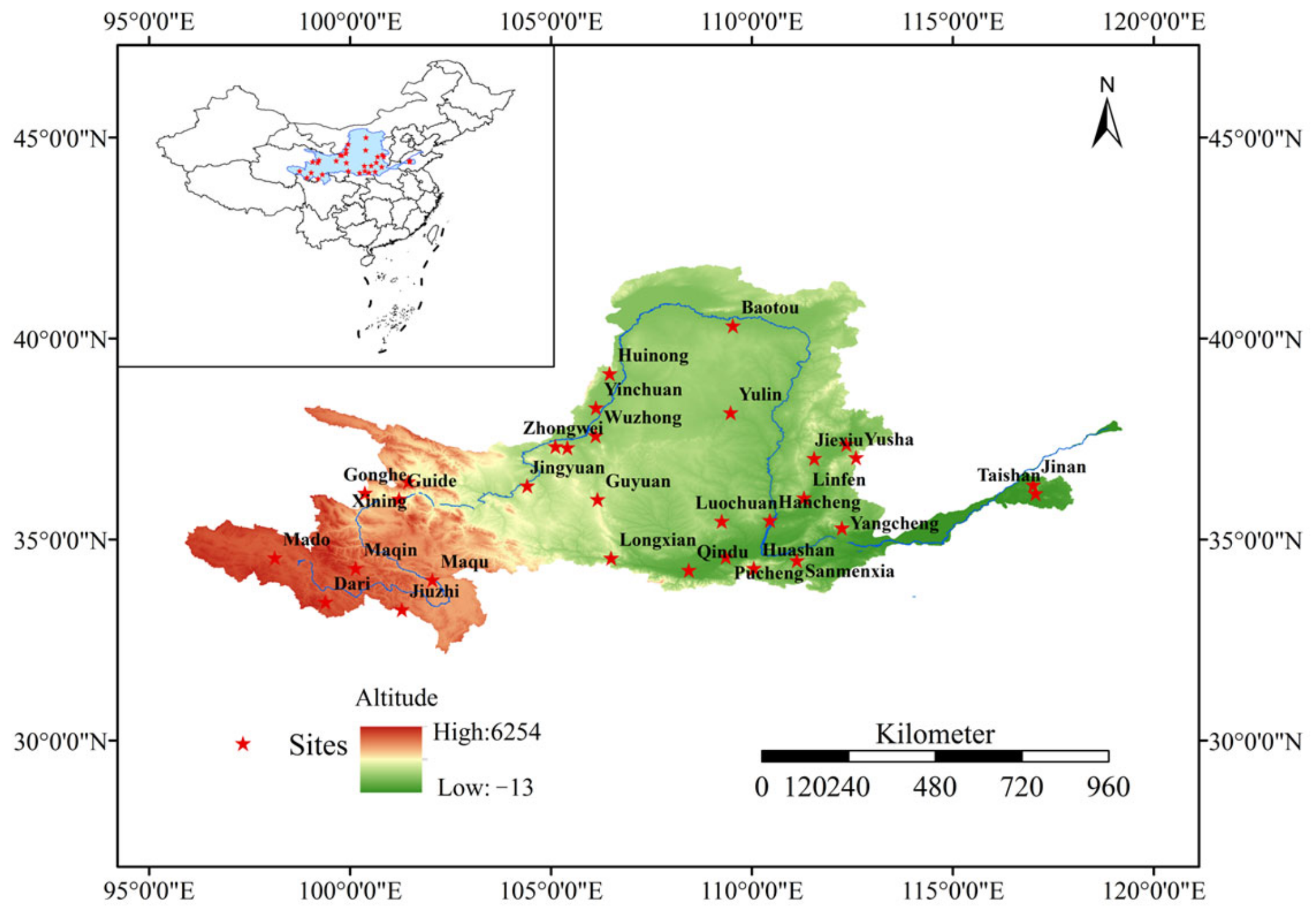
This study fully accounts for the topographic and climatic heterogeneity within the basin. A total of 31 meteorological stations were selected, covering the major provinces traversed by the Yellow River, including Qinghai, Gansu, Ningxia, Inner Mongolia, Shaanxi, Shanxi, Henan, and Shandong. These stations are representative of the upper and middle reaches of the basin (Figure 1), with detailed information provided in Table 1.
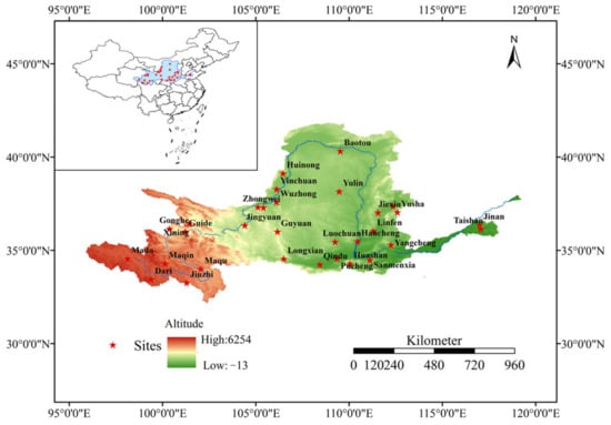
Figure 1.
Map of study area and representative meteorological stations.

Table 1.
Climatic zonation of meteorological stations in Yellow River Basin.
2.2. Data Acquisition and Preprocessing
2.2.1. Meteorological Data
This study obtained daily scale meteorological data for the period from 1 January 1960 to 31 December 2023 for the meteorological stations listed in Table 1 from the China Meteorological Data Service Center (http://data.cma.cn, accessed on 11 November 2024) [25]. The dataset includes daily maximum temperature (Tmax), minimum temperature (Tmin), mean temperature (Tmean), average wind speed at 2 m (WS), minimum wind speed, minimum relative humidity, average relative humidity (RH), and sunshine duration (SSH). The raw meteorological data were preprocessed by setting upper and lower threshold values for each variable based on historical meteorological records in the Yellow River Basin. A reasonable threshold method based on the 3σ rule was used to detect and remove outliers in the meteorological data. For each variable, values falling outside three standard deviations from the mean were considered abnormal and excluded. Short-term missing values (≤10 days) were filled using linear interpolation to ensure data continuity and completeness. Data segments with continuous missing values exceeding 10 days were removed to maintain the reliability of subsequent ET0 calculations and model training.
2.2.2. Climatic Zonation
In this study, an unsupervised learning method, K-means clustering, was employed to classify the meteorological stations within the Yellow River Basin. This method partitioned the dataset into K mutually exclusive clusters by minimizing the within-cluster variance. The core objective was to iteratively optimize cluster centroids such that the Euclidean distance between each data point and the centroid of its assigned cluster was minimized. K-means clustering effectively captured the natural distribution patterns within the data and enabled the reasonable grouping of meteorological stations based on key climatic variables [26]. Since climatic zonation required the integration of multiple meteorological factors, the K-means approach allowed for data-driven classification without relying on subjective rules, thereby enhancing the scientific rigor and objectivity of the zonation results.
The objective function of the K-means algorithm can be expressed as
In the objective function above, K denotes the number of clusters, represents the j-th data point, is the centroid of the i-th cluster, and refers to the set of data points belonging to cluster i. The term represents the squared Euclidean distance between a data point and its corresponding cluster centroid. To determine the optimal value of K, this study adopted the Elbow Method, which involves plotting the relationship between K and the within-cluster sum of squares (WCSS). As K increases, WCSS gradually decreases, but the rate of decrease slows down. The optimal K is identified at the “elbow point” of the curve, where the marginal gain in reduced WCSS begins to diminish. This approach ensures a balance between clustering performance and model complexity [27].
In this study, the long-term mean values of four key meteorological variables—Tmean, RH, WS, and SSH—from 31 meteorological stations across the Yellow River Basin were selected as input features for clustering. The detailed results of the climatic zonation are presented in Table 1.
2.2.3. Drought Year Identification
This study obtained monthly scale Standardized Precipitation–Evapotranspiration Index (SPEI) data for the Yellow River Basin from 1960 to 2023 via the Google Earth Engine platform (https://developers.google.com/earth-engine/datasets, accessed on 11 November 2024) [28]. The SPEI accounts for the combined effects of precipitation and evapotranspiration on drought conditions, making it a widely used tool for drought detection and monitoring [29]. For the purpose of this study, the 12-month-timescale SPEI (SPEI-12) was selected to reflect annual water surplus and deficit conditions. Spatial interpolation techniques were used to align the data with the selected meteorological stations within the basin. Based on previous research, years with an annual SPEI-12 value less than −1 were defined as dry years, while those with SPEI-12 ≥ −1 were considered non-dry years. This classification was used to distinguish between drought and non-drought years over the study period. The drought years for each climatic zone are listed in Table 2; all years not mentioned in the table are considered non-drought years.
Table 2.
Summary of dry years by climatic zone.
2.3. ET0 Calculation Method
2.3.1. Penman–Monteith Equation
The PM equation, recommended by the FAO as the standard method for calculating ET0 in FAO-56, is widely applied in agricultural and hydrological research. This method integrates both energy balance and aerodynamic components, allowing for the accurate simulation of the evapotranspiration process of reference crops [30]. The PM equation is expressed as follows:
In the equation, is the net radiation (MJ/(m2d)); is the soil heat flux (MJ·m2/d), which was set to 0 in this study as calculations were on a daily scale; is the wind speed at a 2 m height (m/s); is the saturation vapor pressure (kPa); is the actual vapor pressure (kPa); is the slope of the saturation vapor pressure–temperature curve (kPa/°C); is the psychrometric constant (kPa/°C); and is the mean air temperature (°C).
In this study, was estimated using measured sunshine duration, station latitude, and elevation, following the FAO-56 method [30]. Incoming solar radiation (Rs) was calculated using the Angstrom formula, with extraterrestrial radiation derived from astronomical parameters. The surface albedo (α) was fixed at 0.23 for reference crop surfaces. was set to zero on a daily timescale, consistent with FAO-56 recommendations. and the psychrometric constant were calculated from air temperature and pressure, with atmospheric pressure adjusted by station elevation. Importantly, wind speed measurements at all stations were obtained at 2.0 m, in accordance with the PM standard, thus eliminating the need for height conversion.
2.3.2. Priestley–Taylor and Hargreaves Equation
The Priestley–Taylor (PT) equation is a simplified version of the PM equation, which assumes that aerodynamic factors—specifically wind speed—have minimal impact on ET0. It is primarily applicable in humid regions or areas with negligible wind variability [31]. The PT equation is expressed as follows:
In the equation, is an empirical coefficient, typically assigned a value of 1.26.
The Hargreaves–Samani (HG) equation is a temperature-based empirical method that estimates ET0 using only diurnal temperature range and solar radiation. It is particularly suitable for data-scarce regions or areas lacking wind speed and humidity measurements [32]. The HG equation is expressed as follows:
In the equation, and represent the daily maximum and minimum air temperatures (°C), respectively. is the extraterrestrial radiation (MJ m−2 day−1), calculated based on the station’s latitude and the day of the year, following FAO-56 procedures [30].
2.3.3. Machine Learning Models
This study employed several regression-based machine learning models—RF, an SVM, GB, and Ridge—to estimate ET0 and to evaluate the applicability of machine learning approaches under varying climatic zones, cross-site settings, and drought conditions [33,34,35,36]. Among them, RF and GB are ensemble algorithms based on decision trees, capable of capturing complex nonlinear relationships with strong fitting capacity. The SVM employs kernel functions to model intricate nonlinear patterns in high-dimensional feature spaces. In contrast, Ridge is a linear model with L2 regularization, serving as a baseline to assess the limitations of linear structures. The inclusion of the Ridge model helped to isolate the contribution of nonlinearity to model accuracy, thereby enabling a clearer comparison of the relative advantages of other models. To ensure model stability and computational accuracy, all input features and target data were subjected to preprocessing.
First, the input features were selected to align with the meteorological variables required for calculating ET0 using the PT and HG equations. Specifically, models compared against the PT equation used Rn, Tmean, and RH as input variables, while models compared against the HG equation used Tmean, Tmax, Tmin, and extraterrestrial radiation (Ra). The ET0 values computed using the PM equation were used as the target variable (label). To eliminate the influence of differing units and to enhance model stability, all input and target data were normalized to a common scale, which also helped accelerate model convergence and improve predictive accuracy. The dataset was divided based on the previously defined climatic zones, with 70% used for training and 30% for validation to ensure regional representativeness. To minimize the impact of seasonal variability, data from all months were evenly sampled so that both training and validation sets captured the full spectrum of annual climatic fluctuations. Hyperparameters for each model were optimized using 10-fold cross-validation within each climatic zone, ensuring robust generalization and performance stability. To evaluate the generalization ability of the models, two strategies were employed in this study. Strategy 1 involved cross-site validation. Specifically, within each climatic zone, one meteorological station was alternately selected as the test set, while the remaining stations in the same zone were used for training. The models were trained using the previously determined optimal hyperparameters. This approach allowed for assessing the capability of different regression models to estimate ET0 across stations within the same climatic conditions, and to identify their respective strengths and limitations. Strategy 2 focused on drought applicability validation. To evaluate model performance under drought stress, a drought-year prediction experiment was conducted. For each climatic zone, data from all meteorological stations during a selected drought year (SPEI ≤ −1.0) were used as the test set, while data from non-drought years within the same zone were used for training. Again, models were trained using the optimized hyperparameters. This strategy enabled the assessment of each model’s ability to estimate ET0 under water-deficit conditions and its applicability in the context of climate change. By comparing the results of the cross-site and drought-year experiments, this study systematically evaluated the ET0 estimation performance of different machine learning models across various climatic zones and moisture conditions and explored the potential and applicability of machine learning approaches to improve ET0 estimation beyond traditional empirical methods.
2.4. Data Analysis and Model Evaluation
2.4.1. Data Analysis
This study performed statistical analyses of ET0 across different climatic zones and meteorological stations. Pearson’s correlation analysis was employed to quantify the linear relationships between ET0 and key meteorological variables, including Tmean, WS, RH, and SSH [37]. The Mann–Kendall (MK) test, a non-parametric trend detection method, was employed to identify statistically significant trends in the data [38]. Compared to traditional trend analysis techniques, the MK test does not assume any specific data distribution and is less sensitive to outliers, making it particularly suitable for analyzing ordinal or categorical time series. It quantitatively assesses the temporal trends of drought indices and other variables. In this study, the standard normal test statistic Z derived from the MK test was used to evaluate trend changes in hydrological indicators and soil moisture over specific periods. Values of ∣Z∣ equal to or exceeding 1.28, 1.64, and 2.32 corresponded to significance levels of 90%, 95%, and 99%, respectively, indicating increasingly strong evidence of statistically significant trends.
2.4.2. Model Evaluation
The coefficient of determination (R2), Root Mean Square Error (RMSE), and Mean Absolute Error (MAE) were used to evaluate model goodness-of-fit, error magnitude, and prediction stability, respectively [39]. The calculation formulas for these three metrics are as follows. Smaller values of the RMSE and MAE indicate better simulation performance, while larger R2 values indicate better simulation performance.
where and are the observed and predicted yield values, respectively; and are the mean values of the observed and predicted values, respectively; and is the number of samples.
3. Results
3.1. Trends in ET0 and Its Influencing Factors in the Yellow River Basin
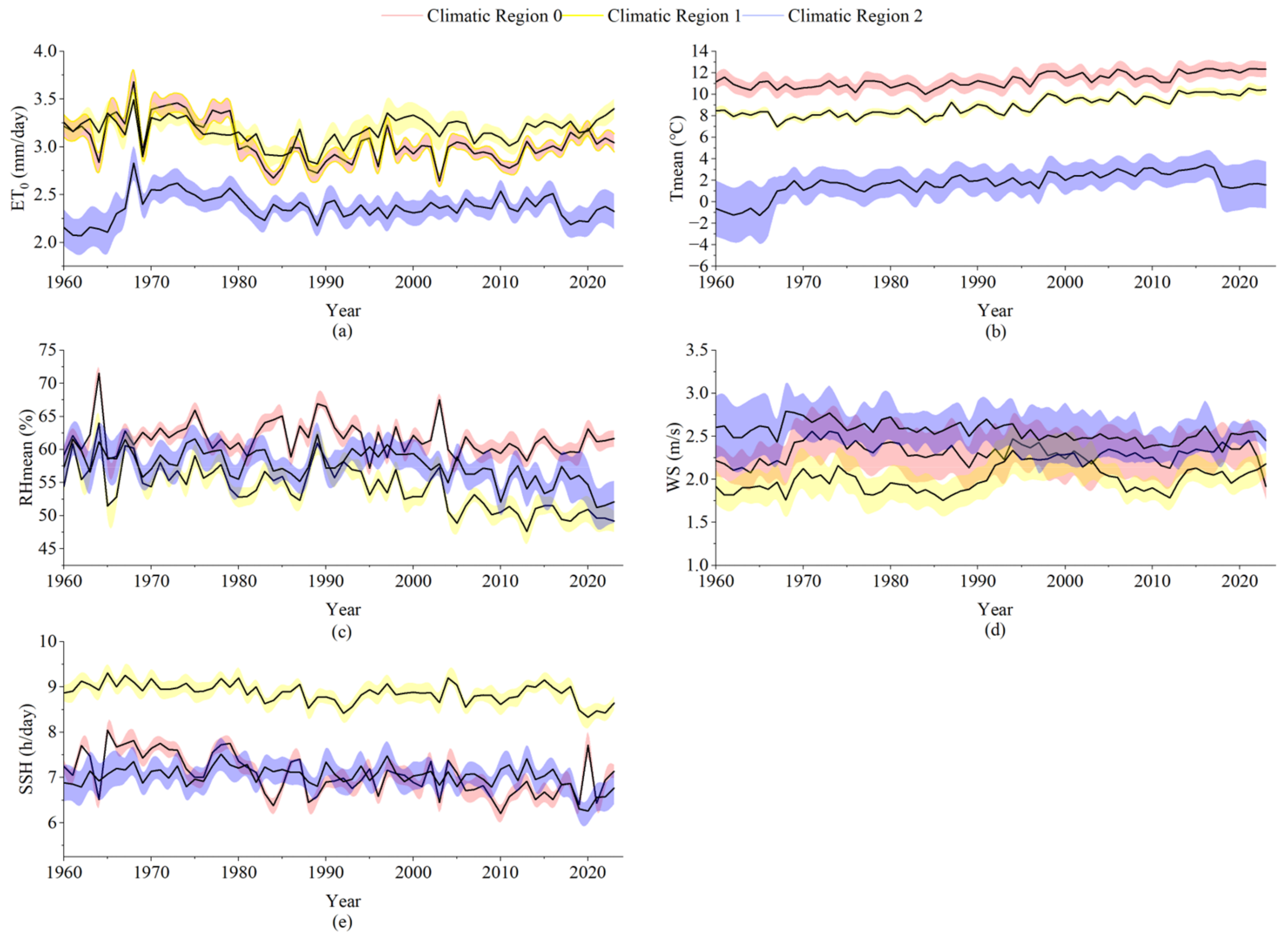
Figure 2 illustrates the interannual variation trends of the annual ET0 and its main influencing factors across different climatic zones in the Yellow River Basin from 1960 to 2023. As shown in Figure 2a, the average ET0 values in Climatic Zones 0 and 1 are consistently higher than those in Climatic Zone 2. The long-term average ET0 in Climatic Zone 0 is 3.05 mm/day, while in Climatic Zone 1 it is 3.17 mm/day, and in Climatic Zone 2, the average is only 2.37 mm/day. Figure 2b shows that the long-term average Tmean in Climatic Zones 0 and 1 is 11.31 °C and 8.89 °C, respectively, significantly higher than the 1.70 °C in Climatic Zone 2. This aligns well with the ET0 differences between the zones, indicating that Climatic Zone 2, due to its higher elevation and lower temperatures, has lower crop water evapotranspiration. Figure 2c,d show the variations in RH and WS. The three climatic zones exhibit minimal differences in these two factors, with long-term average RH values generally staying between 50 and 65%, and WS averaging between 2.0 and 2.5 m/s. Figure 2e illustrates the interannual trend of SSH. It can be observed that Climatic Zone 1 consistently shows significantly higher SSH throughout the entire time series, with a long-term average of 8.87 h/day, notably higher than the 7.06 h/day in Climatic Zone 0 and 7.02 h/day in Climatic Zone 2. This may be attributed to the geographic and climatic conditions in Climatic Zone 1, which is inland, has fewer clouds, and is at a moderate elevation, all of which enhance the potential evapotranspiration driven by solar radiation.
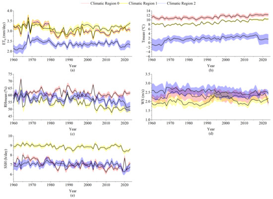
Figure 2.
Trends in ET0 and meteorological factors. Note: (a–e) represent the interannual variations of reference evapotranspiration, mean temperature, relative humidity, wind speed at 2 m, and sunshine duration in each climatic zone, respectively.
According to the Mann–Kendall (MK) trend test results for meteorological factors and ET0 from 1960 to 2023 in each climatic zone, as shown in Table 3, the Tmean in all three climatic zones shows a significant increasing trend, with Z-values of 6.10 (Climatic Zone 0), 7.34 (Climatic Zone 1), and 5.96 (Climatic Zone 2), all passing the 99% confidence level significance test. This indicates that the rise in temperature is a widespread climate change characteristic in the Yellow River Basin. Relative Humidity (RH) shows a significant decreasing trend in all three climatic zones, with Z-values of −1.62, −5.90, and −4.63, with Climatic Zone 1 showing the most significant decline. The trend of WS varies between climatic zones: Climatic Zone 0 shows a slight increase (Z = 0.17), Climatic Zone 1 exhibits a significant increase (Z = 2.71), while Climatic Zone 2 shows a decreasing trend (Z = −4.81). For SSH, all three climatic zones show a significant decreasing trend, with Z-values of −4.85, −3.81, and −2.18. As for ET0, the overall trend varies: Climatic Zones 0 and 2 show significant and slight decreases (Z = −2.39, −0.53), respectively, while Climatic Zone 1 shows a slight increase (Z = 0.18), although it did not pass the significance test. This suggests that the response of ET0 to climatic factor changes differs notably across climatic zones.
Table 3.
Mann–Kendall (MK) trend test for meteorological data and ET0 changes from 1960 to 2023.
3.2. Comparison of Machine Learning Models and PT Equation
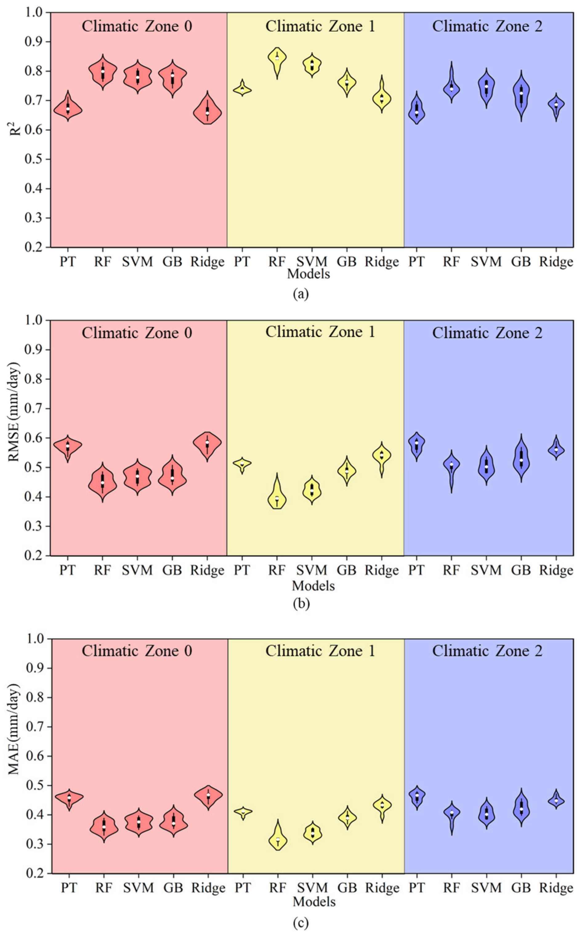
Figure 3 presents a comparison of the simulation accuracy between the PT empirical equation and several machine learning models (RF, SVR, GB, and Ridge) under Strategy 1 across three climatic zones. Overall, the PT model showed significant disadvantages in all climatic zones, with an average R2 of only 0.68, an RMSE of 0.57 mm/day, and an MAE of 0.45 mm/day. Compared to the RF, SVM, and GB machine learning models, the PT model’s R2 was lower by 0.09, and its RMSE and MAE were higher by 0.09 and 0.07, respectively. However, it was only 0.003 lower in R2 than the Ridge model, and both the RMSE and MAE were higher by 0.002 mm/day. This indicates that the relationship between ET0 and meteorological data is nonlinear, and the PT formula has weak nonlinear response capability, making it less suitable for estimation across multiple climatic conditions. From the perspective of climatic zone differences, the average R2 values of all models were higher in Climatic Zone 0, with the RF model performing the best, reaching an average R2 of 0.80. The accuracy of the SVM and GB models was slightly lower, while the Ridge model had the lowest accuracy with an R2 of 0.66. In Climatic Zones 1 and 2, the performance of all models slightly decreased, but the simulation accuracy of the machine learning methods still outperformed that of the PT model. It is evident that machine learning models offered superior error control, with the RF and SVM models consistently showing lower average errors across all climatic zones. Therefore, compared to the PT equation, the machine learning models demonstrated stronger fitting ability and stability across multiple climatic regions.
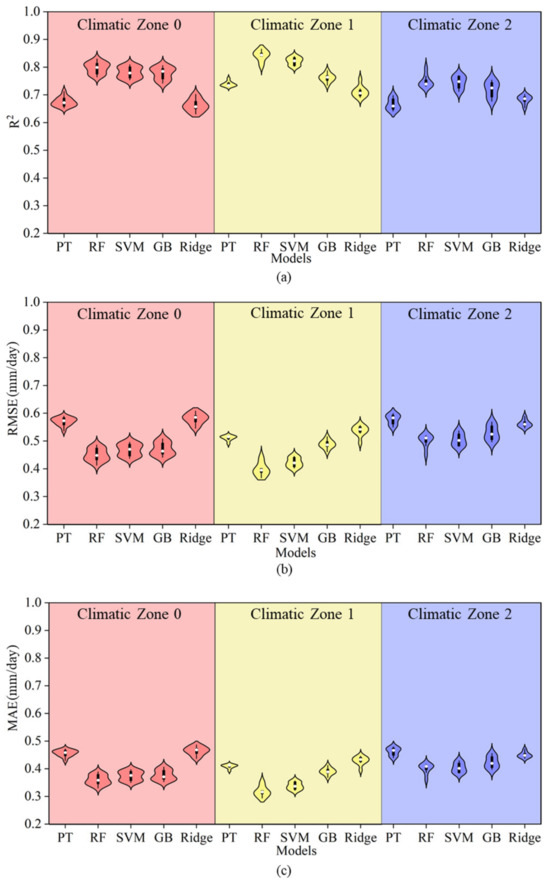
Figure 3.
A comparison of accuracy between the PT equation and machine learning models under Strategy 1. Note: Different colors in the figure represent different climatic zones. Panels (a–c) show the R2, RMSE, and MAE of each model under Strategy 1 within each climatic zone, respectively, along with comparisons to the PT model.
Figure 4 presents a comparison between the PT empirical equation and several machine learning models (RF, SVR, GB, and Ridge) under Strategy 2 in drought years. In this scenario, the PT model estimated an average R2 of 0.67, RMSE of 0.57 mm/day, and MAE of 0.46 mm/day for drought years. In comparison, the RF, SVM, and GB models exhibited an average R2 increase of 0.05 over the PT model, with the RMSE and MAE decreasing by 0.05 and 0.03, respectively, demonstrating higher precision. However, the Ridge model showed a decrease in the average R2 by 0.04, with the RMSE and MAE increasing by 0.03 and 0.02, respectively, compared to the PT model. Moreover, compared to Figure 3, the estimation accuracy of the PT model for ET0 in drought years did not change significantly, while the simulation accuracy of the machine learning models decreased by varying extents. The R2 of the RF and SVM models decreased by 0.04 compared to those in Strategy 1, and both the GB and Ridge models saw a decrease of 0.05.
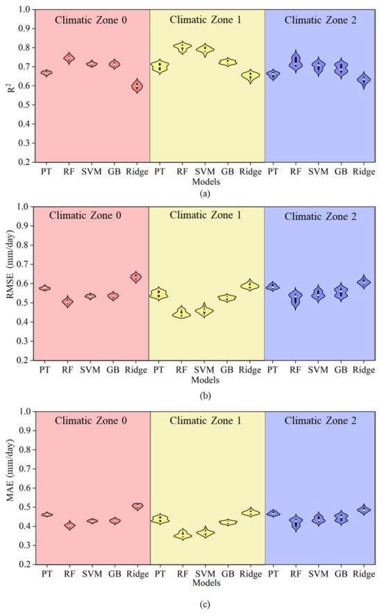
Figure 4.
A comparison of accuracy between the PT equation and machine learning models under Strategy 2. Note: Different colors in the figure represent different climatic zones. Panels (a–c) show the R2, RMSE, and MAE of each model under Strategy 2 within each climatic zone, respectively, along with comparisons to the PT model.
3.3. Comparison of Machine Learning Models and the HG Equation
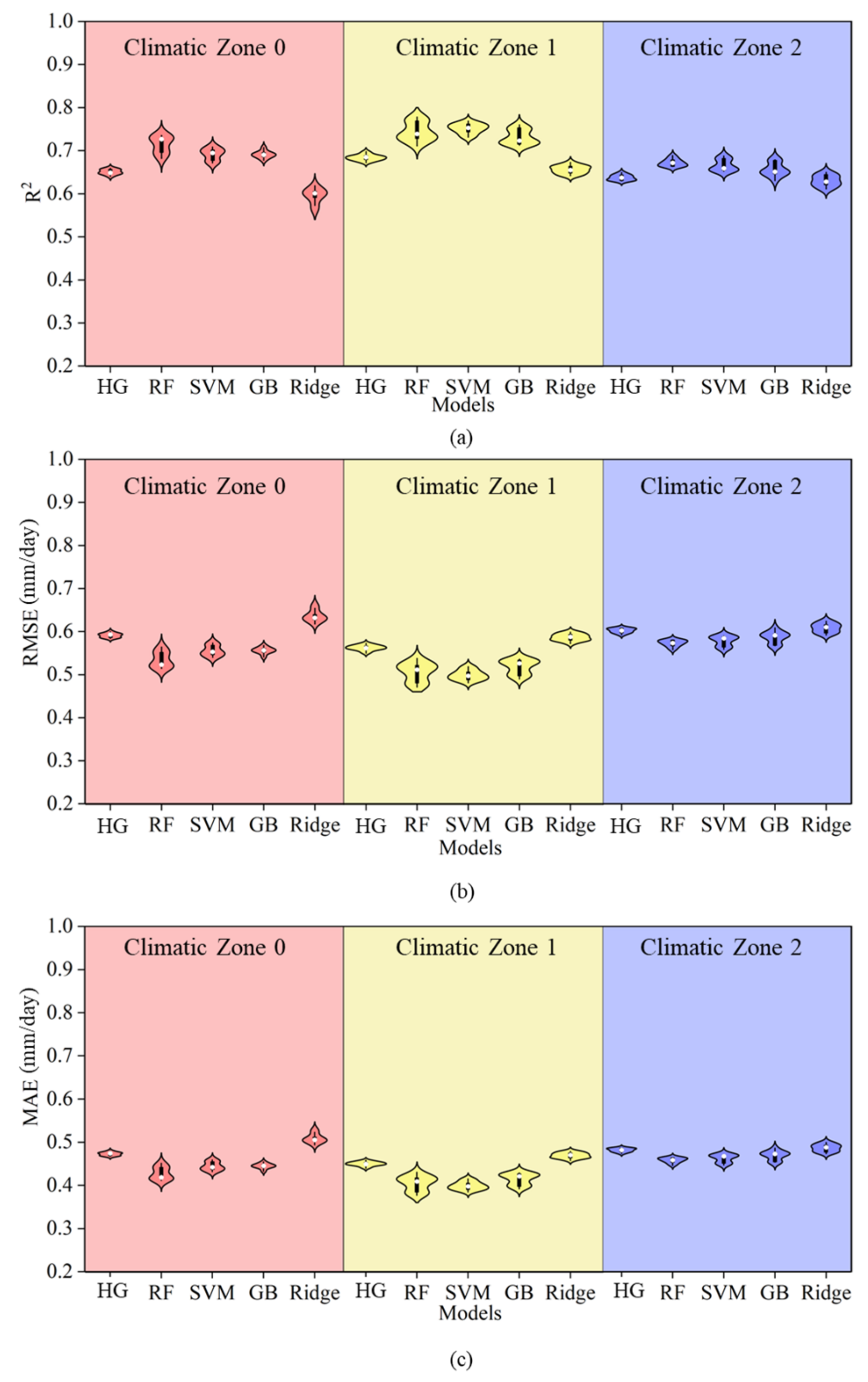
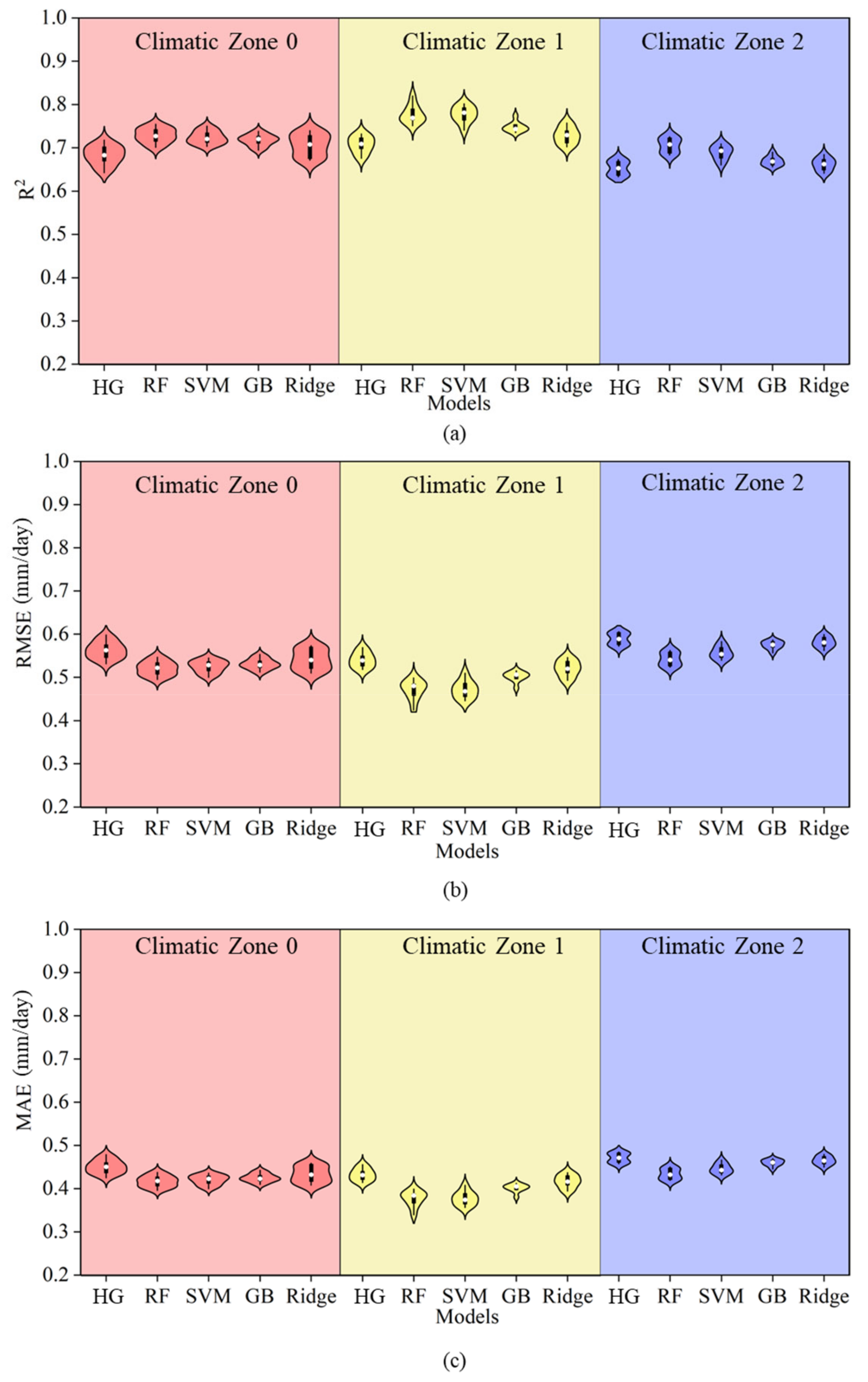
Figure 5 presents a comparison of the simulation accuracy between the HG empirical equation and several machine learning models (RF, SVR, GB, and Ridge) under Strategy 1 across three climatic zones. Among these, the HG model demonstrated the lowest simulation accuracy for ET0, with an average R2 0.04 lower than that of the RF, SVM, and GB machine learning models and an RMSE and MAE higher by 0.04 and 0.03, respectively. However, its R2 was only 0.02 lower than that of the Ridge model, while its RMSE and MAE are higher by 0.07 mm/day. This indicates that, similarly to the PT equation, the meteorological factors used in the HG formula also exhibited a nonlinear relationship with ET0, and the HG formula’s ability to respond to nonlinearity is weak, making it less suitable for estimation under these climatic conditions. In terms of climatic zone differences, the average R2 values of all models were higher in Climatic Zone 1, with the RF model performing the best, achieving an average R2 of 0.78. The precision of the SVM and GB models was slightly lower, while the Ridge model exhibited the lowest precision with an R2 of 0.73. In Climatic Zones 0 and 2, the performance of all models slightly declined, but the simulation accuracy of the machine learning methods remained superior to that of the HG model. This shows that, compared to the HG equation, the machine learning models—especially the nonlinear models—demonstrated stronger fitting ability and stability across multiple climatic regions.

Figure 5.
A comparison of accuracy between the HG equation and machine learning models under Strategy 1. Note: Different colors in the figure represent different climatic zones. Panels (a–c) show the R2, RMSE, and MAE of each model under Strategy 1 within each climatic zone, respectively, along with comparisons to the HG model.
Figure 6 presents a comparison between the HG empirical equation and several machine learning models (RF, SVR, GB, and Ridge) under Strategy 2 in drought years. In this scenario, the HG model estimated an average R2 of 0.66, RMSE of 0.58 mm/day, and MAE of 0.47 mm/day for drought years. In comparison, the RF, SVM, and GB models showed an average R2 increase of 0.05 over the HG model, with the RMSE and MAE decreasing by 0.04 mm/day and 0.03 mm/day, respectively, demonstrating higher precision. However, the Ridge model showed a decrease in average R2 by 0.03 compared to the PT model, with the RMSE and MAE increasing by 0.02 mm/day. Moreover, compared to that shown in Figure 5, the ET0 estimation accuracy of the HG model in drought years did not change significantly, while the simulation accuracy of the machine learning models decreased by varying extents. The R2 of the RF and SVM models decreased by 0.02 compared to those in Strategy 1, that of the GB model decreased by 0.01, and that of the Ridge model showed the largest decrease of 0.07.

Figure 6.
A comparison of accuracy between the HG equation and machine learning models under Strategy 2. Note: Different colors in the figure represent different climatic zones. Panels (a–c) show the R2, RMSE, and MAE of each model under Strategy 2 within each climatic zone, respectively, along with comparisons to the HG model.
Based on the evaluation results in Section 3.2 and Section 3.3, the random forest (RF) model consistently demonstrated superior performance under various climate zones and drought conditions. It achieved higher R2 and lower RMSE and MAE values compared to other machine learning models, indicating greater stability and generalization ability, especially in data-scarce or highly variable environments. Therefore, in the subsequent analysis, we selected the RF model as the representative machine learning method to compare it with traditional empirical models and evaluate its practical applicability under diverse climatic scenarios.
3.4. Error Between Simulated and Observed Values
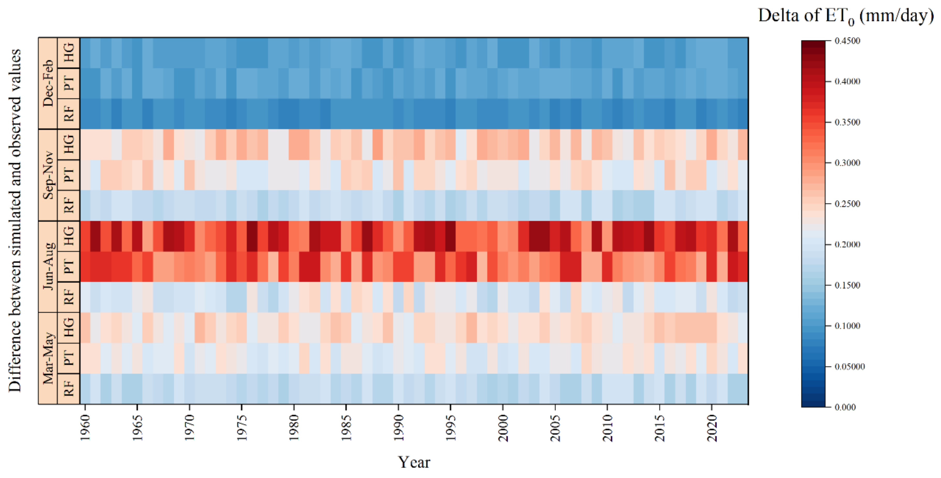
Figure 7 illustrates the dynamic variation in the differences between various ET0 estimation methods (RF, PT, and HG) and the standard values across different seasons from 1960 to 2023. Overall, the RF model showed smaller estimation deviations throughout the year compared to the PT and HG equations. The average annual deviation of ET0 estimated by the RF model was reduced by 0.057 mm/day and 0.076 mm/day compared to that of the PT and HG models, respectively, demonstrating better accuracy and stability. From a seasonal perspective, the period from June to August showed the most significant differences, with the annual average differences between the PT and HG models and the standard values being 0.328 mm/day and 0.366 mm/day, respectively. In contrast, the RF model significantly reduced the estimation bias during this season to 0.207 mm/day, decreasing by 0.121 mm/day and 0.159 mm/day compared to that of the PT and HG models, respectively. This highlights the RF model’s significant optimization ability for ET0 estimation during the peak evapotranspiration season with high temperatures. Conversely, during the winter months from December to February, the differences between the models and the standard values were the smallest. The annual average differences for RF, PT, and HG were 0.090 mm/day, 0.111 mm/day, and 0.108 mm/day, respectively, indicating that the ET0 variation was smaller in winter, and all models maintained high consistency.

Figure 7.
Dynamic variation in differences between various ET0 estimation methods and standard values for different seasons from 1960 to 2023.
4. Discussion
4.1. Comparison of ET0 Estimation Accuracy Under Strategy 1
Under Strategy 1, all machine learning models generally outperformed the traditional empirical formulas PT and HG in ET0 estimation accuracy across different climatic zones. Specifically, using the PM equation as a baseline, nonlinear models such as RF, the SVM, and GB achieved an average R2 of 0.77, with an RMSE and MAE of 0.49 mm/day and 0.38 mm/day, respectively, across the three climatic zones. In contrast, the PT model had an average R2 of only 0.68, with an RMSE and MAE of 0.57 mm/day and 0.45 mm/day, respectively. In comparison, the RF model increased R2 by 0.09 and reduced the RMSE and MAE by 0.08 mm/day and 0.07 mm/day, respectively, showing a clear advantage. The slightly weaker linear model, Ridge, had an R2 almost identical to that of the PT model (only differing by 0.003) but still exhibited smaller errors in the RMSE and MAE. The primary reason for this difference is the complex nonlinear relationship between ET0 and the input meteorological factors. As fixed-structure empirical formulas, both PT and HG models have limited expressive capability when facing interactions and changes in input variables [40]. Despite using the same input features as PT and HG formulas, the machine learning models constructed in this study, thanks to their nonlinear fitting abilities and stronger feature relationship modeling capabilities, could more effectively uncover hidden coupling relationships and nonlinear response processes between meteorological factors, thus providing higher-precision ET0 estimates under the same input conditions [41]. This result aligns with the findings of Feng, et al. [42] and Tabari, et al. [43]. This indicates that even when the feature dimensions are limited, the flexibility of the model structure and the fitting mechanism still play a significant role in ET0 estimation performance [44].
Additionally, compared to the PT model, the HG model performed slightly worse in this study. The average R2 of the HG model was 0.04 lower than that of PT, with the RMSE and MAE higher by 0.04 mm/day and 0.03 mm/day, respectively. This finding is consistent with the results of Chen, et al. [45]. A possible reason for this phenomenon is that the HG formula mainly relies on the diurnal temperature range and radiation empirical function, failing to accurately reflect ET0’s sensitivity to changes in radiation intensity. This is particularly true in regions with abundant sunshine but large temperature fluctuations, where estimation biases can be amplified. In contrast, while the PT formula also does not explicitly consider wind speed and humidity, it uses net radiation as the primary driving factor, which can more realistically represent the control of energy supply on evapotranspiration. Therefore, it performed slightly better in the study area [46]. Further analysis revealed that machine learning models based on the input variables required by the HG formula had an average R2 of about 0.73, which was higher than that of the HG formula itself but still lower than that of the machine learning models trained with PT input variables (average R2 of about 0.77). This suggests that even with machine learning methods, the representativeness and completeness of input factors still significantly influenced model performance.
In conclusion, nonlinear machine learning models, with their powerful feature learning and generalization capabilities, significantly improved ET0 estimation accuracy across multiple climatic regions. The selection of model input variables also played a crucial role, indicating that even within the same machine learning framework, the combination of meteorological factors could significantly affect model performance [47]. This conclusion is consistent with related findings from other regions and further validates the feasibility and superiority of using machine learning methods for ET0 estimation in regions with limited data quality and availability [48].
4.2. Impact of Drought Stress on Model Accuracy in ET0 Estimation
From the simulation results under Strategy 2, it is evident that the simulation accuracy of traditional empirical formulas, the PT and HG models, showed relatively small variation compared to in normal years, demonstrating a certain degree of robustness. Specifically, the R2 of the PT model decreased slightly from 0.68 under Strategy 1 to 0.67, a reduction of only 0.01, while the RMSE and MAE remained at 0.57 mm/day and 0.46 mm/day, with minimal changes. Similarly, the HG model maintained similar stability, with R2 increasing from 0.64 to 0.66, showing a slight recovery. The RMSE and MAE were 0.58 mm/day and 0.47 mm/day, respectively. This suggests that under drought stress, the PT and HG formulas, due to their simple computational structure and low dependence on input variables, were less affected by abnormal disturbances in meteorological factors, maintaining relatively consistent estimation capabilities [49].
In contrast, most machine learning models showed a noticeable decrease in estimation accuracy during drought years. The average R2 of the RF model decreased from 0.77 under Strategy 1 to 0.73, a decrease of 0.04. The R2 values of the SVR and GB models decreased by 0.04 and 0.05, respectively, showing more significant performance deterioration. The most noticeable decline was observed in the Ridge model, whose R2 decreased by 0.07 under drought conditions, while the RMSE and MAE increased by 0.07 mm/day and 0.06 mm/day, respectively. Its accuracy even fell below that of the PT and HG models in this scenario. This was mainly because the response mechanisms between meteorological variables changed during drought years, causing the relationships between variables learned during the training process to no longer apply to the drought context, thereby affecting the model’s generalization ability [50]. Especially for linear regression models like Ridge, their sensitivity to changes in input variable relationships is higher, and they lack the adaptability to non-typical climatic contexts [51]. In contrast, formulas like PT and HG, due to their fixed model structure and lack of reliance on data learning processes, are more robust under extreme conditions [52]. Moreover, during drought years, the increased variation in some meteorological factors could lead to a shift in the input feature distribution of machine learning models, affecting prediction performance. This is particularly true when the proportion of drought year samples in the training set is low, which can cause “generalization weakening” in the model [53].
Therefore, although machine learning models demonstrate higher accuracy under normal climatic conditions, their estimation ability faces some risk of decline under extreme drought scenarios. Improvements can be made by increasing the drought sample size, introducing more robust model structures, or adopting ensemble learning techniques. The results of this study highlight that when constructing regional-scale ET0 estimation models, drought response capability should be considered a key factor to improve the model’s applicability in the context of increasingly frequent extreme climate events in the future.
4.3. Uncertainty and Perspectives
Although this study systematically evaluated the applicability of various ET0 estimation models across different climatic zones and under drought conditions at the regional scale, there are still certain uncertainties that need to be addressed and expanded upon in future research. First, the estimation accuracy of machine learning models in drought years still requires improvement, particularly as some models exhibit significant performance degradation under extreme drought conditions. The main reason for this phenomenon is the limited number of samples during drought years, which prevents the models from fully learning the nonlinear response patterns of meteorological factors under water stress conditions during the training phase. Therefore, future research should focus on accumulating meteorological observation data from extreme climate event years and constructing a high-quality sample database covering a wider range of climatic backgrounds and drought intensities, thus enhancing the models’ adaptability to extreme conditions.
Secondly, this study primarily focused on ET0 as the estimation target, without extending further to the simulation and validation of actual evapotranspiration. It is influenced by multiple factors, such as crop type, management practices, and soil moisture conditions, and has more direct practical significance for agricultural water resource management. Therefore, future studies could build upon ET0 estimation by incorporating vegetation indices, crop coefficients (Kc), or actual crop observational data, enabling the dynamic conversion and estimation from ET0 to ETa, thereby enhancing the application value of the research findings.
In addition, although this study primarily evaluated the HG model as a temperature-based empirical reference, we acknowledge that other simplified models such as Turc and Jensen-Haise may provide complementary perspectives, especially in humid climate zones where solar radiation and humidity play a more significant role [54]. However, considering that the Yellow River Basin is predominantly semi-arid to arid, and the main focus of this study was on data-scarce and drought-prone regions, the HG and PT models were prioritized due to their relevance in such environments [55]. Nonetheless, we fully recognize the value of including other temperature- or radiation-based models for broader benchmarking. If deemed necessary, we are willing to incorporate additional simplified models such as the Turc or Jensen-Haise models in future work to further enhance the comprehensiveness of the model comparison.
5. Conclusions
This study focused on analyzing the differences in the applicability and variation characteristics of the models under different climatic zones and drought conditions. The machine learning models using the same meteorological variables as the PT and HG formulas generally exhibited higher estimation accuracy in most scenarios. Using the PM equation estimates as the benchmark, the nonlinear machine learning models (RF, SVR, GB) consistently outperformed the linear Ridge model, with the RF model performing the best across all climatic zones. Its R2 reached 0.77, significantly higher than that of the PT (R2 = 0.68) and HG (R2 = 0.64) models. The average annual ET0 estimation error was reduced by 0.057 mm/day and 0.076 mm/day compared to PT and HG, respectively, with the accuracy advantage being particularly significant during the high-temperature and high-evapotranspiration season from June to August. In the drought year scenario, the estimation accuracy of the PT and HG models remained stable, with R2 values of 0.67 and 0.66, respectively. However, the R2 of the machine learning models decreased by an average of 0.05, though they were still higher than those of the PT and HG models. The Ridge model, however, shows a 0.07 decrease in R2 for ET0 estimation in drought years, with accuracy lower than that of traditional empirical formulas. This indicates that the nonlinear machine learning models based on simplified meteorological factors exhibited good accuracy, applicability, and stability in ET0 estimation. The results of this study provide theoretical support and technical references for agricultural irrigation scheduling, water resource optimization, and drought risk early warning in the Yellow River Basin. This study is limited by its site-specific dataset and may not fully generalize to other regions or crops. Future work should expand to diverse agroecological zones and consider more variables to improve model robustness.
Author Contributions
J.Z.: Data curation; Formal analysis; Methodology; Writing—original draft. H.Z.: Supervision; Writing—original draft; Writing—review & editing. C.W.: Supervision; Writing—review & editing; Funding acquisition. All authors have read and agreed to the published version of the manuscript.
Funding
This work was supported by the 111 Project of China (No. D20015), which is gratefully acknowledged.
Data Availability Statement
Data will be made available on request.
Acknowledgments
The authors would like to give special thanks to the anonymous reviewers.
Conflicts of Interest
We declare that we have no financial and personal relationships with other people or organizations that can inappropriately influence our work, there is no professional or other personal interest of any nature or kind in any product, service and/or company that could be construed as influencing the position presented in, or the review of, the manuscript entitled.
References
- Li, L.; Liu, J.; Peng, Q.; Wang, X.; Xu, J.; Cai, H. Propagation process-based agricultural drought typology and its copula-based risk. Irrig. Drain. 2024, 73, 1496–1519. [Google Scholar] [CrossRef]
- Qin, C.; Guo, W.; Liu, Y.; Liu, Z.; Qiu, J.; Peng, J. A novel electrochemical sensor based on graphene oxide decorated with silver nanoparticles–molecular imprinted polymers for determination of sunset yellow in soft drinks. Food Anal. Methods 2017, 10, 2293–2301. [Google Scholar] [CrossRef]
- Kenawy, A.E.; Al-Awadhi, T.; Abdullah, M.; Ostermann, F.O.; Abulibdeh, A. A Multidecadal Assessment of Drought Intensification in the Middle East and North Africa: The Role of Global Warming and Rainfall Deficit. Earth Syst. Environ. 2025, 1–20. [Google Scholar] [CrossRef]
- Yang, Z.; Solangi, Y.A. Analyzing the relationship between natural resource management, environmental protection, and agricultural economics for sustainable development in China. J. Clean. Prod. 2024, 450, 141862. [Google Scholar] [CrossRef]
- Yan, H.; Acquah, S.J.; Zhang, J.; Wang, G.; Zhang, C.; Darko, R.O. Overview of modelling techniques for greenhouse microclimate environment and evapotranspiration. Int. J. Agric. Biol. Eng. 2021, 14, 1–8. [Google Scholar] [CrossRef]
- Zhang, C.; Li, L.; Yan, H.; Ou, M.; Akhlaq, M.; Zhang, W.; Huang, S. Calibration and validation of three evapotranspiration models in a tea field in the humid region of south-east China. Irrig. Drain. 2022, 71, 1254–1267. [Google Scholar] [CrossRef]
- Ippolito, M.; De Caro, D.; Cannarozzo, M.; Provenzano, G.; Ciraolo, G. Evaluation of daily crop reference evapotranspiration and sensitivity analysis of FAO Penman-Monteith equation using ERA5-Land reanalysis database in Sicily, Italy. Agric. Water Manag. 2024, 295, 108732. [Google Scholar] [CrossRef]
- Allen, R.G.; Pruitt, W.O.; Wright, J.L.; Howell, T.A.; Ventura, F.; Snyder, R.; Itenfisu, D.; Steduto, P.; Berengena, J.; Yrisarry, J.B. A recommendation on standardized surface resistance for hourly calculation of reference ETo by the FAO56 Penman-Monteith method. Agric. Water Manag. 2006, 81, 1–22. [Google Scholar] [CrossRef]
- Monteith, J.L. Evaporation and environment. Proc. Symp. Soc. Exp. Biol. 1965, 19, 205–234. [Google Scholar]
- Penman, H.L. Natural evaporation from open water, bare soil and grass. Proc. R. Soc. Lond. Ser. A Math. Phys. Sci. 1948, 193, 120–145. [Google Scholar]
- Sentelhas, P.C.; Gillespie, T.J.; Santos, E.A. Evaluation of FAO Penman–Monteith and alternative methods for estimating reference evapotranspiration with missing data in Southern Ontario, Canada. Agric. Water Manag. 2010, 97, 635–644. [Google Scholar] [CrossRef]
- Córdova, M.; Carrillo-Rojas, G.; Crespo, P.; Wilcox, B.; Célleri, R. Evaluation of the Penman-Monteith (FAO 56 PM) method for calculating reference evapotranspiration using limited data. Mt. Res. Dev. 2015, 35, 230–239. [Google Scholar] [CrossRef]
- Vakili, M.; Sabbagh-Yazdi, S.R.; Khosrojerdi, S.; Kalhor, K. Evaluating the effect of particulate matter pollution on estimation of daily global solar radiation using artificial neural network modeling based on meteorological data. J. Clean. Prod. 2017, 141, 1275–1285. [Google Scholar] [CrossRef]
- Utset, A.; Farre, I.; Martínez-Cob, A.; Cavero, J. Comparing Penman–Monteith and Priestley–Taylor approaches as reference-evapotranspiration inputs for modeling maize water-use under Mediterranean conditions. Agric. Water Manag. 2004, 66, 205–219. [Google Scholar] [CrossRef]
- Shi, W.; Zhang, X.; Xue, X.; Feng, F.; Zheng, W.; Chen, L. Analyzing Evapotranspiration in Greenhouses: A Lysimeter-Based Calculation and Evaluation Approach. Agronomy 2023, 13, 3059. [Google Scholar] [CrossRef]
- Valiantzas, J.D. Temperature-and humidity-based simplified Penman’s ET0 formulae. Comparisons with temperature-based Hargreaves-Samani and other methodologies. Agric. Water Manag. 2018, 208, 326–334. [Google Scholar] [CrossRef]
- Bishop, K.; Shanley, J.B.; Riscassi, A.; de Wit, H.A.; Eklöf, K.; Meng, B.; Mitchell, C.; Osterwalder, S.; Schuster, P.F.; Webster, J. Recent advances in understanding and measurement of mercury in the environment: Terrestrial Hg cycling. Sci. Total Environ. 2020, 721, 137647. [Google Scholar] [CrossRef]
- Sun, M.; Yuan, W.; Liu, N.; Jia, L.; Wu, F.; Huang, J.-H.; Wang, X.; Feng, X. Combined Impacts of Climate and Tree Physiology on Mercury Accumulation in Tropical and Subtropical Foliage and Robust Model Parametrization. Environ. Sci. Technol. 2025, 59, 1661–1672. [Google Scholar] [CrossRef]
- Dong, C.; Zhu, H.; Wang, J.; Yuan, H.; Zhao, J.; Chen, Q. Prediction of black tea fermentation quality indices using NIRS and nonlinear tools. Food Sci. Biotechnol. 2017, 26, 853–860. [Google Scholar] [CrossRef]
- Han, F.; Huang, X.; Teye, E. Novel prediction of heavy metal residues in fish using a low-cost optical electronic tongue system based on colorimetric sensors array. J. Food Process Eng. 2019, 42, e12983. [Google Scholar] [CrossRef]
- Sládek, D.; Marková, L.; Talhofer, V. Towards Sustainable Urban Mobility: Leveraging Machine Learning Methods for QA of Meteorological Measurements in the Urban Area. Sustainability 2024, 16, 5713. [Google Scholar] [CrossRef]
- Yong, S.L.S.; Ng, J.L.; Huang, Y.F.; Ang, C.K. Estimation of reference crop evapotranspiration with three different machine learning models and limited meteorological variables. Agronomy 2023, 13, 1048. [Google Scholar] [CrossRef]
- Wang, G.; Yang, Y. Quantitative evaluation of digital economy policy in Heilongjiang Province of China based on the PMC-AE index model. Sage Open 2024, 14, 21582440241234435. [Google Scholar] [CrossRef]
- Shi, H.; Luo, G.; Hellwich, O.; Xie, M.; Zhang, C.; Zhang, Y.; Wang, Y.; Yuan, X.; Ma, X.; Zhang, W. Evaluation of water flux predictive models developed using eddy-covariance observations and machine learning: A meta-analysis. Hydrol. Earth Syst. Sci. 2022, 26, 4603–4618. [Google Scholar] [CrossRef]
- Available online: http://data.cma.cn (accessed on 11 November 2024).
- Huan, J.; Cao, W.; Liu, X. A dissolved oxygen prediction method based on k-means clustering and the elm neural network: A case study of the Changdang Lake, China. Appl. Eng. Agric. 2017, 33, 461–469. [Google Scholar] [CrossRef]
- Likas, A.; Vlassis, N.; Verbeek, J.J. The global k-means clustering algorithm. Pattern Recognit. 2003, 36, 451–461. [Google Scholar] [CrossRef]
- Available online: https://developers.google.com/earth-engine/datasets (accessed on 11 November 2024).
- Lin, H.; Xu, P.T.; Sun, L.; Bi, X.k.; Zhao, J.w.; Cai, J.r. Identification of eggshell crack using multiple vibration sensors and correlative information analysis. J. Food Process Eng. 2018, 41, e12894. [Google Scholar] [CrossRef]
- Allen, R.G. Using the FAO-56 dual crop coefficient method over an irrigated region as part of an evapotranspiration intercomparison study. J. Hydrol. 2000, 229, 27–41. [Google Scholar] [CrossRef]
- Shuttleworth, W.J.; Calder, I.R. Has the Priestley-Taylor equation any relevance to forest evaporation? J. Appl. Meteorol. Climatol. 1979, 18, 639–646. [Google Scholar] [CrossRef]
- Talebmorad, H.; Ahmadnejad, A.; Eslamian, S.; Ostad-Ali-Askari, K.; Singh, V.P. Evaluation of uncertainty in evapotranspiration values by FAO56-Penman-Monteith and Hargreaves-Samani methods. Int. J. Hydrol. Sci. Technol. 2020, 10, 135–147. [Google Scholar] [CrossRef]
- Iranzad, R.; Liu, X. A review of random forest-based feature selection methods for data science education and applications. Int. J. Data Sci. Anal. 2024, 1–15. [Google Scholar] [CrossRef]
- Yu, S.; Ren, Y.; Wu, X.; Guo, P.; Li, Y. Dynamic pruning-based Bayesian support vector regression for reliability analysis. Reliab. Eng. Syst. Saf. 2024, 244, 109922. [Google Scholar] [CrossRef]
- Wijayanti, E.B.; Setiadi, D.R.I.M.; Setyoko, B.H. Dataset analysis and feature characteristics to predict rice production based on eXtreme gradient boosting. J. Comput. Theor. Appl. 2024, 1, 299–310. [Google Scholar] [CrossRef]
- Kelly, H.R.; Sreekumar, S.; Manee, V.; Cuomo, A.E.; Newhouse, T.R.; Batista, V.S.; Buono, F. Ligand-Based Principal Component Analysis Followed by Ridge Regression: Application to an Asymmetric Negishi Reaction. ACS Catal. 2024, 14, 5027–5038. [Google Scholar] [CrossRef]
- Cheng, J.; Sun, J.; Yao, K.; Dai, C. Generalized and hetero two-dimensional correlation analysis of hyperspectral imaging combined with three-dimensional convolutional neural network for evaluating lipid oxidation in pork. Food Control 2023, 153, 109940. [Google Scholar] [CrossRef]
- McLeod, A.I. Kendall rank correlation and Mann-Kendall trend test. R Package Kendall 2005, 602, 1–10. [Google Scholar]
- Ouyang, Q.; Zhao, J.; Pan, W.; Chen, Q. Real-time monitoring of process parameters in rice wine fermentation by a portable spectral analytical system combined with multivariate analysis. Food Chem. 2016, 190, 135–141. [Google Scholar] [CrossRef]
- Zhao, S.; Chen, Z.; Xiong, Z.; Shi, Y.; Saha, S.; Zhu, X.X. Beyond Grid Data: Exploring graph neural networks for Earth observation. IEEE Geosci. Remote Sens. Mag. 2024, 13, 175–208. [Google Scholar] [CrossRef]
- Niranjan, S.; Nandagiri, L. Effect of local calibration on the performance of the Hargreaves reference crop evapotranspiration equation. J. Water Clim. Change 2021, 12, 2654–2673. [Google Scholar] [CrossRef]
- Feng, Y.; Cui, N.; Zhao, L.; Hu, X.; Gong, D. Comparison of ELM, GANN, WNN and empirical models for estimating reference evapotranspiration in humid region of Southwest China. J. Hydrol. 2016, 536, 376–383. [Google Scholar] [CrossRef]
- Tabari, H.; Kisi, O.; Ezani, A.; Talaee, P.H. SVM, ANFIS, regression and climate based models for reference evapotranspiration modeling using limited climatic data in a semi-arid highland environment. J. Hydrol. 2012, 444, 78–89. [Google Scholar] [CrossRef]
- Rajput, J.; Singh, M.; Lal, K.; Khanna, M.; Sarangi, A.; Mukherjee, J.; Singh, S. Data-driven reference evapotranspiration (ET0) estimation: A comparative study of regression and machine learning techniques. Environ. Dev. Sustain. 2024, 26, 12679–12706. [Google Scholar] [CrossRef]
- Chen, Z.; Zhu, Z.; Jiang, H.; Sun, S. Estimating daily reference evapotranspiration based on limited meteorological data using deep learning and classical machine learning methods. J. Hydrol. 2020, 591, 125286. [Google Scholar] [CrossRef]
- Katul, G.G.; Oren, R.; Manzoni, S.; Higgins, C.; Parlange, M.B. Evapotranspiration: A process driving mass transport and energy exchange in the soil-plant-atmosphere-climate system. Rev. Geophys. 2012, 50. [Google Scholar] [CrossRef]
- Haider, S.T.; Ge, W.; Li, J.; Rehman, S.U.; Imran, A.; Sharaf, M.; Haider, S.M. An Ensemble Machine Learning Framework for Cotton Crop Yield Prediction Using Weather Parameters: A Case Study of Pakistan. IEEE Access 2024, 12, 124045–124061. [Google Scholar] [CrossRef]
- Bariş, M.; Tombul, M. A review on models, products and techniques for evapotranspiration measurement, estimation, and validation. Environ. Qual. Manag. 2024, 34, e22250. [Google Scholar] [CrossRef]
- Nandgude, N.; Singh, T.; Nandgude, S.; Tiwari, M. Drought prediction: A comprehensive review of different drought prediction models and adopted technologies. Sustainability 2023, 15, 11684. [Google Scholar] [CrossRef]
- Hao, Z.; Singh, V.P.; Xia, Y. Seasonal drought prediction: Advances, challenges, and future prospects. Rev. Geophys. 2018, 56, 108–141. [Google Scholar] [CrossRef]
- Fridley, J.D.; Vandermast, D.B.; Kuppinger, D.M.; Manthey, M.; Peet, R.K. Co-occurrence based assessment of habitat generalists and specialists: A new approach for the measurement of niche width. J. Ecol. 2007, 95, 707–722. [Google Scholar] [CrossRef]
- Shen, C.; Appling, A.P.; Gentine, P.; Bandai, T.; Gupta, H.; Tartakovsky, A.; Baity-Jesi, M.; Fenicia, F.; Kifer, D.; Li, L. Differentiable modelling to unify machine learning and physical models for geosciences. Nat. Rev. Earth Environ. 2023, 4, 552–567. [Google Scholar] [CrossRef]
- Briceno-Mena, L.A.; Arges, C.G.; Romagnoli, J.A. Machine learning-based surrogate models and transfer learning for derivative free optimization of HT-PEM fuel cells. Comput. Chem. Eng. 2023, 171, 108159. [Google Scholar] [CrossRef]
- Tan, L.; Zheng, K.; Zhao, Q.; Wu, Y. Evapotranspiration estimation using remote sensing technology based on a SEBAL model in the upper reaches of the Huaihe river basin. Atmosphere 2021, 12, 1599. [Google Scholar] [CrossRef]
- Shahid, M.; Khalid, S.; Bibi, I.; Bundschuh, J.; Niazi, N.K.; Dumat, C. A critical review of mercury speciation, bioavailability, toxicity and detoxification in soil-plant environment: Ecotoxicology and health risk assessment. Sci. Total Environ. 2020, 711, 134749. [Google Scholar]

Disclaimer/Publisher’s Note: The statements, opinions and data contained in all publications are solely those of the individual author(s) and contributor(s) and not of MDPI and/or the editor(s). MDPI and/or the editor(s) disclaim responsibility for any injury to people or property resulting from any ideas, methods, instructions or products referred to in the content. |
© 2025 by the authors. Licensee MDPI, Basel, Switzerland. This article is an open access article distributed under the terms and conditions of the Creative Commons Attribution (CC BY) license (https://creativecommons.org/licenses/by/4.0/).