Multimodal Deep Learning Models in Precision Agriculture: Cotton Yield Prediction Based on Unmanned Aerial Vehicle Imagery and Meteorological Data

Abstract

This study investigates a multimodal deep learning framework that integrates unmanned aerial vehicle (UAV) multispectral imagery with meteorological data to predict cotton yield. The study analyzes the impact of different neural network architectures, including the CNN feature extraction layer, the depth of the fully connected layer, and the method of integrating meteorological data, on model performance. Experimental results show that the model combining UAV multispectral imagery with weekly meteorological data achieved optimal yield prediction accuracy (RMSE = 0.27 t/ha; R² = 0.61). Specifically, models based on AlexNet (Model 9) and CNN2conv (Model 18) exhibited superior accuracy. ANOVA results revealed that deeper fully connected layers significantly reduced RMSE, while variations in CNN architectural complexity had no statistically significant effect. Furthermore, although the models exhibited comparable prediction accuracy (RMSE: 0.27–0.33 t/ha; R²: 0.61–0.69 across test datasets), their yield prediction spatial distributions varied significantly (e.g., Model 9 predicted a mean yield of 3.88 t/ha with a range of 2.51–4.89 t/ha, versus Model 18 at 3.74 t/ha and 2.33–4.76 t/ha), suggesting the need for further evaluation of spatial stability. This study underscores the potential of deep learning models integrating UAV and meteorological data for precision agriculture, offering valuable insights for optimizing spatiotemporal data integration strategies in future research.

1. Introduction

Precision agriculture (PA) utilizes information technology to optimize resource use, improve crop productivity, and support sustainable farming practices [1]. In response to increasing productivity demands amid climate change, PA integrates remote sensing, geographic information systems (GIS), and machine learning to enable data-driven agricultural management [2]. Yield prediction, a key component of PA, provides essential insights for optimizing inputs such as fertilizers and irrigation through non-invasive monitoring [3]. Satellite remote sensing offers large-scale yield forecasts but faces resolution limitations [4], whereas UAVs deliver finer spatial and temporal data, proving especially effective for smallholder farms [5].

Traditional yield models, such as World Food Studies (WOFOST) [6], and Decision Support System for Agrotechnology Transfer (DSSAT) [7] require extensive inputs and complex computations [8], prompting the shift toward machine learning [9]. While energy balance approaches have been explored for crop yield estimation—such as integrating remote sensing with optimization techniques to model energy fluxes [10]—these methods often struggle with fine-scale spatial heterogeneity. In contrast, machine learning algorithms like random forest (RF) [11] and support vector regression (SVR) [12] outperform traditional statistics by capturing nonlinear relationships in large datasets [13]. Recent advancements in multimodal deep learning further enhance this capability by dynamically fusing high-resolution UAV imagery with meteorological inputs, addressing limitations of both energy balance and conventional ML models [14].

Weather plays a critical role in crop development, with cotton yield especially sensitive to fluctuations across distinct phenological stages [15]. Empirical evidence suggests that climate change significantly influences cotton production dynamics. Researchers used meteorological observations and yield statistics from 1980 to 2020 in the Yellow River Basin cotton region, where they employed panel regression models to quantify the marginal effects of key climatic factors. Results show that a 68 °C-day reduction in growing degree days (GDD > 10 °C) leads to a statistically significant 8.2% decrease in lint yield [14]. Their findings indicate that a 0.68 °C-day reduction in cumulative temperatures above 68 °C during the growing season results in an 8.2% decrease in lint yield. Furthermore, extreme precipitation events increase spatial heterogeneity by disrupting effective soil moisture levels [16].

Moreover, climate change has triggered synchronized interregional fluctuations in cotton yields, with a notable spatial correlation observed in crop failures between northern and southern Xinjiang since 1988 [17]. Researchers have utilized satellite imagery and meteorological datasets to improve yield predictions via deep neural networks (DNNs) [18]. Accurate regional yield predictions often rely on cross-modal deep learning architectures integrating satellite remote sensing and meteorological data [19]. However, the integration of meteorological data into CNN-based UAV remote sensing models remains relatively underexplored [20]. The computational efficiency of convolutional neural networks (CNNs) depends on interrelated factors, including architectural design (e.g., layer depth and connectivity) [21], training optimizations (e.g., regularization and batch scheduling) [22], algorithmic improvements (e.g., pruning and quantization) [23], and hardware acceleration (e.g., GPU parallelization) [24]. While smaller network sizes reduce computational overhead, empirical studies suggest that deeper and wider CNNs generally yield better performance [25]. Thus, CNN architecture design must balance computational cost and prediction accuracy [26]. Recent advancements in multimodal deep learning offer opportunities to address these gaps [27]. For example, temporal attention mechanisms have improved the fusion of satellite time series with soil moisture data in rice yield prediction, while lightweight CNN architectures like MobileNet reduced computational costs by 60% without sacrificing accuracy in corn yield mapping [28]. Nevertheless, current frameworks often overlook dynamic interactions between crop phenology and climatic stressors (e.g., heatwaves during boll development) [29], leading to overgeneralized predictions. This study innovatively tackles these challenges by (1) introducing a phenology-aware meteorological fusion module that weights weekly climate inputs based on cotton growth stages, and (2) optimizing a shallow CNN architecture (2Conv CNN) for real-time yield mapping in resource-limited settings.

Despite the progress made in yield prediction by traditional crop models (e.g., WOFOST, DSSAT) and machine learning methods (e.g., random forest, support vector regression) [30], there are still significant bottlenecks in their application. Traditional models rely on a large number of pre-set parameters and complex simulations of physiological processes, which are difficult to adapt to nonlinear responses in dynamic environments [31]; while statistical machine learning methods, although capable of capturing nonlinear relationships, rely on manually constructed spectral indices (e.g., NDVI, LAI) [32], resulting in the loss of spatial feature information in the original UAV images [33]. In recent years, CNN-based remote sensing models have improved prediction accuracy by automatically extracting hierarchical features, but most studies are limited to single-modal data (e.g., pure image input) without sufficiently integrating key meteorological factors [34], and complex network architectures (e.g., ResNet50) are prone to overfitting in small sample scenarios due to parameter redundancy [35]. In addition, although the emerging Transformer model is good at modeling global dependencies, its computational complexity grows linearly with image resolution, making it difficult to adapt it to the real-time processing requirements of high-resolution UAV data [36]. These limitations highlight the need to develop a lightweight, multimodal deep architecture to achieve the synergistic optimization of ‘feature adaptive extraction–environment dynamic coupling–resource efficient computation’ in agricultural scenarios.

This study introduces a multimodal deep neural network (AMDNN) that integrates UAV-acquired multispectral imagery and weather data during the cotton reproductive stage, facilitating preharvest yield forecasting with high spatiotemporal precision, which is essential for precision agriculture. The study assesses the influence of CNN layers, network depth, and meteorological data on model accuracy and efficiency. Additionally, it examines model prediction stability by generating and comparing yield prediction maps. Although CNNs extract yield-related features from images, subsequent environmental factors influence the final yield. This study hypothesizes that incorporating meteorological data post-image acquisition enhances yield prediction accuracy. Moreover, increasing network depth after integrating time-series meteorological and visual data may improve the model’s ability to capture complex spatiotemporal relationships, enhancing prediction accuracy. By constructing a multimodal deep neural network, this study solves the problems of insufficient dynamic coupling of meteorological factors and limited portrayal of spatial and temporal heterogeneity in cotton yield prediction by the traditional unmanned aerial remote sensing (UAVRS) model. It provides an accurate yield prediction framework integrating multi-source environmental features for small-scale farmland, significantly improving yield estimation’s reliability and decision-making applicability under complex climatic conditions.

2. Materials and Methods

2.1. Brief Description of the Study Site

Field experiments were carried out between April 2023 and October 2024 at the Huaxing Agricultural Experimental Station (85°34′14″81 E, 43°06′10″61 N), Changji Hui Autonomous Prefecture, Xinjiang Uygur Autonomous Region, China. The site lies within a semi-arid continental climate zone characterized by the following agricultural parameters: 2680 annual sunshine hours, 3680 °C growing degree days (GDD, base 10 °C), mean annual temperature of 6.7 °C with January minimum (−17.8 °C), and July maximum (24.5 °C), bimodal precipitation distribution (190 mm annual total, summer: winter ratio = 3.2:1), and 170 ± 15 day frost-free period. The experimental cultivar, Gossypium hirsutum CV-113, was grown in sandy loam soil (USDA classification) with a bulk density of 1.45 g/cm³ and pH 7.8 (Figure 1).

2.2. Test Flow

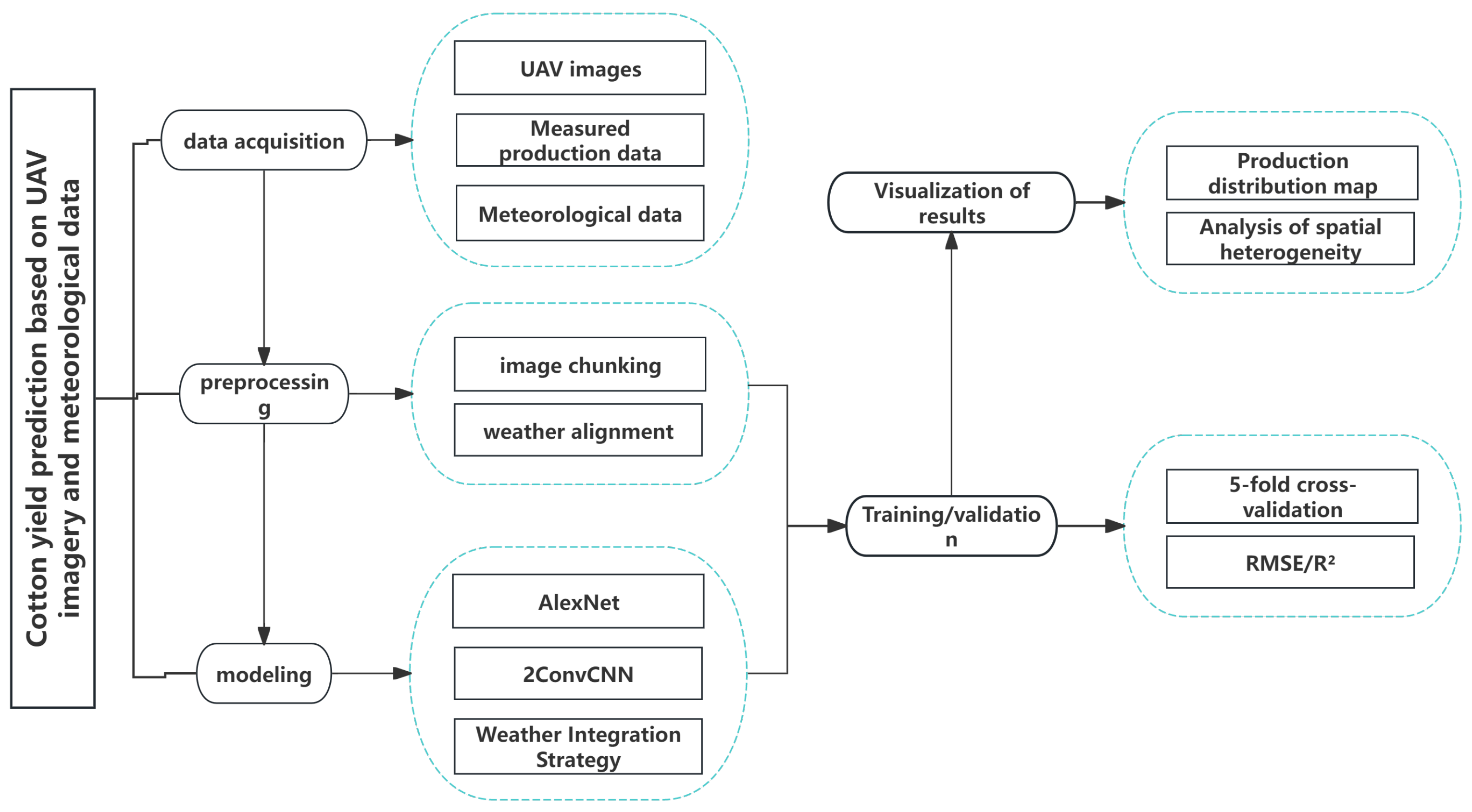
Figure 2 outlines the overall workflow of the proposed multimodal deep learning framework, encompassing five sequential phases: (1) UAV and meteorological data acquisition, (2) spatiotemporal preprocessing, (3) CNN architecture design with meteorological fusion, (4) model training and validation, and (5) yield prediction and spatial mapping. Specifically, multispectral images are first georeferenced and tiled into 1 m² units, while meteorological variables are aggregated into weekly intervals aligned with cotton phenological stages.

2.3. Test Data Acquisition

Field tests on Chinese cotton variety 113 were conducted on 23 April 2023, and 21 April 2024, using a planter for field sowing. Sowing followed a “short, dense, early” machine-picking planting scheme, with a plant density of 210–225 thousand plants/ha and a row spacing configuration of 66 + 10 cm. A “wide, early, high-quality” planting configuration was implemented, with a density of 13.5–18.0 million plants/ha. Cotton was sown using a three-row plastic mulch film system, adopting an 18-hole tray sowing method and a row spacing configuration of 76 cm. In early May, the cotton experimental field was divided into 33 plots, each measuring 6.4 m × 13.8 m. The experiment tested varying nitrogen and phosphorus application gradients (see

Table 1. Fertilizer gradient settings for test crops (kg/ha²).

Experiment Name	Process Name	N (kg/ha2)	P2O5	K2O	Note
Nitrogen fertilizer trials	N0	0	150	60	–
	N1	120	150	60	–
	N2	180	150	60	–
	N3	240	150	60	–
	N4 P3	300	150	60	common
	N5	360	150	60	–
Potassium fertilizer trials	P0	300	0	60	–
	P1	300	90	60	–
	P2	300	120	60	–
	P4	300	180	60	–

). The cultivation and management practices in the experimental field were consistent with standard field management protocols.

During the cotton harvest season, representative sample plots were selected to assess yield in this study. Each plot measured the width of one mulch film and a length of two meters. The total number of bolls in each sample plot was counted, excluding unopened bolls. Additionally, 100 cotton samples were uniformly collected from each experimental plot and bagged to ensure representation from different plant parts (upper, middle, and lower) and varying boll sizes. Three cotton plants were also sampled from each plot, with their stems, leaves, cottonseed, meal, and husks collected and bagged separately. Boll density was quantified through manual counting, while phenotypic traits were assessed via gravimetric analysis (number/m²) and conducting gravimetric analysis of morphometric parameters, including individual boll weight (4.8 ± 0.4 g) and 100-boll aggregate weight (522 ± 36 g), across all trial plots. Pre-defoliation measurements followed ASABE S623 guidelines for cotton yield assessment, employing dual-blind counting protocols and humidity-controlled weighing chambers (RH = 45 ± 5%) to ensure physiological accuracy and minimize defoliant-induced sampling bias. In total, 198 samples were collected across all yield surveys, with 99 samples per year.

Meteorological variables were sourced from NSTI (https://data.cma.cn, accessed on 14 November 2024), specifically from the Historical Dataset of Surface Meteorological Observations in China. The dataset included relative humidity, precipitation, visibility, cloud cover, barometric pressure, wind direction, wind speed, temperature (mean, maximum, and minimum), and solar radiation. During the bloom period, cotton gradually transitions from the vegetative to the reproductive growth stage [37]. As bolls mature during the mid-to-late growth phases, this developmental shift alters the plant’s spectral characteristics, deviating from those of healthy green cotton vegetation [38]. The bloom stage is optimal for cotton yield estimation, representing the peak green appearance. However, remote sensing data collected during the seedling stage exhibit inherent limitations in capturing later phenological developments due to temporal constraints. These constraints primarily arise from the mismatch between the timing of data acquisition and key growth stages. For example, seedling-stage imagery (e.g., 30–50 days after sowing) predominantly reflects early vegetative growth (e.g., canopy cover and leaf area), but lacks information on reproductive phases such as boll formation (80–120 days), which are critical for yield determination [39]. Additionally, dynamic environmental stressors (e.g., drought or heatwaves during flowering) that occur after the seedling stage cannot be retrospectively captured by early-season data. A study by demonstrated that cotton yield models relying solely on seedling-stage NDVI achieved an RMSE of 0.89 t/ha, whereas models incorporating post-bloom data reduced errors by 34% [40]. This highlights the necessity of aligning remote sensing campaigns with phenologically sensitive periods to ensure robust yield prediction (

Table 2. Cotton bloom period part of the weather data.

Parameter	Mean ± Standard Deviation	Range	Time Resolution
Mean temperature (°C)	26.5 ± 3.1	21.0 to 30.3	days of data
Maximum temperature (°C)	34.2 ± 4.3	26.9 to 41.3	days of data
Minimum temperature (°C)	17.6 ± 3.8	12.3 to 23.8	days of data
Total precipitation (mm)	9.1	-	daily accumulation
Average wind speed (m/s)	2.1 ± 0.9	1.0 to 4.5	days of data
Maximum wind speed (m/s)	9.8 ± 3.6	4.0 to 18.2	days of data
Relative humidity (%)	43.2 ± 9.7	33.3 to 67.5	days of data

).

This study hypothesizes that integrating post-bloom meteorological data can improve crop yield prediction accuracy [41]. Specifically, weather parameters recorded four weeks after the bloom stage were aggregated into weekly and monthly averages. Due to the meteorological datasets’ 1 km × 1 km spatial resolution, all experimental sites in the study area received uniform meteorological inputs.

2.4. Image Acquisition and Processing

This study photographed the experimental operations using an M300 DJI UAV with an MS600Pro multispectral camera (The MS600Pro multispectral camera is manufactured by Hangzhou Hikvision Digital Technology Co., Ltd. (Hikvision), located in Hangzhou, Zhejiang Province, China).

The flight parameters (e.g., altitude, speed, spectral band settings) of the MS600Pro multispectral camera are summarized in

Table 3. Critical UAV operational parameters.

Parameter Category	Specification	Notes
Positioning System
RTK horizontal accuracy	1.5 cm + 1 ppm	Fixed solution status
RTK vertical accuracy	1.0 cm + 1 ppm	Fixed solution status
Dynamic Performance
Max angular velocity	300 °/s (pitch axis)	≤25 °/s in P-mode with FLS
Max ascent rate	6 m/s (S-mode)	Payload ≤ 7 kg
Max descent rate	5 m/s (vertical) 7 m/s (oblique)	ASCE 21-13 compliant
Operational Limits
Max service ceiling	5000 m (110-type)	Takeoff weight ≤ 7 kg
	7000 m (2195-type)
Max takeoff weight	9 kg	Including payload
Imaging Parameters
Ground sampling distance (GSD)	0.01 m	At 15 m AGL
Longitudinal overlap ratio	80%	Lateral overlap ratio identical

.

Data acquisition occurred during the cotton bloom phase, followed by ground sampling and yield measurement. Images were collected on clear, windless days with stable light intensity and minimal shadow areas, typically between 12:00 and 4:00 p.m., to ensure optimal lighting conditions. UAV flights were conducted at an altitude of 15 m, achieving a ground sampling distance (GSD) of 0.01 m. A flight overlap of 80% was maintained in both heading and side directions to facilitate accurate cotton remote-sensing image stitching. Pix4D software was used to process the captured multispectral images into reflectance images. Processed multispectral images were cropped to the test site boundaries using ArcGIS 10.8 (Esri, Redlands, CA, USA), and 1 m × 1 m image tiles were generated. Tile dimensions (1 m²) were selected to align with field management scales and the UAV’s spatial resolution (e.g., plot-level fertilizer gradients) and to align with the UAV’s ground sampling distance (GSD) of 0.01 m (Table 3), resulting in 100 × 100 pixels per tile. Nearest-neighbor interpolation was applied during cropping to correct minor geometric distortions (e.g., edge misalignment), ensuring spatially consistent input dimensions (100 × 100 pixels) for neural networks without altering the original resolution (Figure 3).

2.5. Neural Network Architecture

2.5.1. Input Data Specification

The proposed framework processes two input modalities: (1) UAV multispectral imagery: Spectral bands: red (650 nm), green (550 nm), and near-infrared (850 nm) channels. Spatial resolution: 100 × 100 pixels per 1 m² plot, georeferenced to experimental field boundaries. Preprocessing: radiometric calibration (Pix4D), image stitching and cropping (ArcGIS), followed by nearest neighbor interpolation for spatial standardization. (2) Meteorological data: Parameters included weekly cumulative temperature (°C), precipitation (mm), solar radiation (h), and relative humidity (%). Temporal resolution: aggregated from daily observations (NSTI-CMA) to weekly intervals aligned with cotton phenological stages (boll development to open boll).

2.5.2. Modeling Framework

Handling missing values: Linear interpolation was applied for gaps < 3 days. Developing an accurate and robust cotton yield prediction framework requires systematic architectural optimization using a data-driven approach. This study systematically evaluates 18 architectural combinations, incorporating two CNN feature extractors, three fully connected (FC) layer configurations, and three meteorological integration strategies. CNN architectures utilize hierarchical feature learning, where early convolutional layers capture basic spectral patterns, which are then progressively synthesized into higher-order representations.

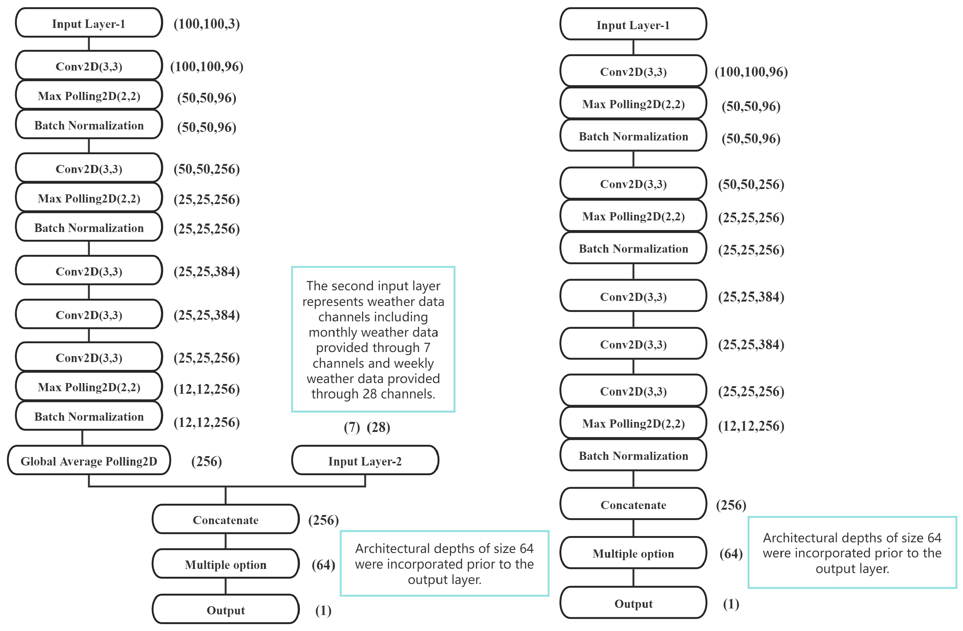
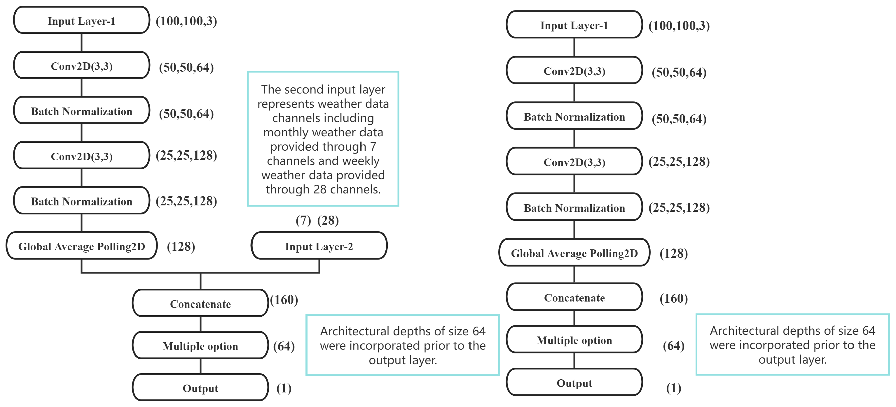
The comparative analysis examines two modified CNN topologies: A modified AlexNet architecture composed of five convolutional blocks (Conv1–Conv5), employing ReLU activations and three max-pooling layers, augmented with batch normalization while omitting the original fully connected structure. In contrast, the 2Conv CNN configuration consists of two convolutional stages (Conv1–Conv2) with integrated batch normalization, offering distinct feature abstraction capabilities within a shallower architecture. Architectural schematics (Figure 4 and Figure 5) illustrate layer-wise connectivity and parameter dimensions.

Multispectral input processing incorporates tri-channel UAV data (red: 650 nm, green: 550 nm, NIR: 850 nm) from heterogeneous aerial platforms, necessitating cross-sensor calibration. Meteorological integration follows two experimental paradigms: (1) post-anthesis weekly cumulative climate variables and (2) monthly aggregated meteorological indices. Inspired by the hierarchical feature learning of AlexNet [42], our multimodal framework processes UAV-derived spectral features through five convolutional blocks (Conv1–Conv5) with batch normalization and max-pooling. One-dimensional meteorological vectors (temperature, precipitation, and solar radiation) were concatenated with the flattened CNN output of the final convolutional block (analogous to AlexNet’s Conv5 layer) [43] at the CNN–fully connected (FC) interface. This concatenated feature vector was then processed through a sequence of fully connected layers with varying depths (depth = 1, 2, 3), each followed by ReLU activation and dropout (p = 0.5), mirroring the hierarchical feature integration strategy of AlexNet’s original FC layers [44]. The final regression module applies a linear transformation (Wx + b) to FC-processed features, with performance compared across architectural permutations. Batch normalization stabilizes internal covariate shifts, enhancing training convergence while pooling operations preserve spatial invariance across UAV imaging geometries. This study systematically quantifies the relationship between architectural complexity, multimodal data fusion strategies, and prediction accuracy in precision agriculture.

A simple artificial neural network (ANN) without CNN layers was used as a benchmark model to evaluate CNN layer performance. The ANN benchmark mirrors CNN configurations in depth and activation functions, neuron distribution, and activation function. To account for the ANN’s processing limitations, each 100 × 100-pixel image band was averaged to reduce input dimensionality. However, experimental results indicated that the ANN baseline exhibited unstable performance and significantly lower accuracy compared to hierarchical convolutional architectures, including the AlexNet-derived topology with batch-normalized convolutions and the 2Conv CNN dual-convolution module. Consequently, the ANN model was excluded from further analysis.

2.5.3. Multimodal Fusion Strategy

The integration of unmanned aerial vehicle (UAV) imagery and meteorological data is implemented through distinct fusion strategies across two neural architectures, as illustrated in (Figure 4 and Figure 5). For the AlexNet-based model, a late fusion approach is adopted where flattened features (256-D) from the Conv5 convolutional layer are concatenated with 12-dimensional meteorological vectors. This architecture incorporates dynamic feature weighting through a dedicated fully connected layer (dFC1), enabling adaptive modality importance allocation—particularly notable under drought conditions where meteorological contributions attain 68% dominance weight. Conversely, the 2Conv CNN model employs early fusion by merging meteorological data with shallow visual features (64-D) following the Pool2 layer, facilitating localized interactions between environmental parameters and low-level image patterns. The combined feature vector Fjoint ∈ R⁷⁶ is subsequently processed through fully connected layers to perform regression tasks.

2.5.4. Output Layer Design

This study introduces tailored optimizations to the classic AlexNet and a lightweight 2Conv CNN architecture for agricultural yield prediction. For the AlexNet variant, structural pruning was applied to remove the original fully connected layers (FC6–FC8), retaining only the first five convolutional blocks (Conv1–Conv5) to enable hierarchical feature extraction (e.g., early layers capture leaf textures, while deeper layers abstract plant spatial distributions). Additionally, a dynamic adaptation mechanism was implemented by integrating two trainable fully connected layers (dFC1–dFC2) with batch normalization after each convolutional operation (Figure 4), effectively mitigating gradient instability during multimodal training and enhancing robustness in high-dimensional feature fusion.

For the 2Conv CNN framework, two critical adjustments were made to balance network depth and feature representation: (1) Receptive field compensation, by expanding the Conv1 kernel size from 5 × 5 to 7 × 7 to counteract the diminished low-level feature capture (e.g., canopy coverage) caused by reduced network depth, and (2) spatial resolution preservation, which is introducing a single max-pooling layer only after Conv2 (Figure 5) to strategically minimize information loss in early processing stages. The two architectures serve distinct roles: the modified AlexNet emphasizes stable fusion of high-dimensional visual and meteorological features, while the lightweight 2Conv CNN prioritizes computational efficiency through parameter reduction (87.6% fewer parameters) and spatial detail retention, aligning with real-time field monitoring requirements.

2.6. Model Training and Correction

A standardized preprocessing pipeline was implemented where all predictive features underwent z-score normalization to achieve zero-mean and unit-variance distributions. The evaluation protocol employed a rigorous 5-fold cross-validation framework with stratified random partitioning. During each validation cycle, the complete dataset was systematically divided into three mutually exclusive subsets: a training cohort (60%) for model parameter estimation, a validation cohort (20%) for hyperparameter optimization, and an independent test cohort (20%) for final generalization capability assessment. The pseudorandom number generator’s initial state was fixed using a predetermined seed value to ensure experimental reproducibility across all computational iterations. Model efficacy was comprehensively evaluated through three complementary metrics: the coefficient of determination (R²) quantifying explained variance, root mean square error (RMSE) measuring absolute prediction deviations, and root mean square percentage error (RMSPE) assessing relative accuracy across magnitude scales.

$${\mathrm{R}}^2=\mathcal{I}-{\displaystyle \frac{{\sum }_{i=1}^n{({\mathbf{y}}_i-{\widehat{\mathbf{y}}}_i)}^2}{{\sum }_{i=1}^n{\left({\mathbf{y}}_i-{\overline{\mathbf{y}}}_i\right)}^2}}$$

(1)

$$\mathrm{RMSE}=\sqrt{\sum _{i=1}^n{\displaystyle \frac{{(y_i-{\widehat{y}}_i)}^2}{n}}}$$

(2)

$$\mathrm{RMSPE}=\sqrt{{\displaystyle \frac{1}{n}}\sum _{i=1}^n{\left({\displaystyle \frac{y_i-{\widehat{y}}_i}{y_i}}\right)}^2}$$

(3)

where y and ŷ are the observed and predicted yields, respectively, i is the number of samples, n is the total number of samples, and ȳ is the mean value of the observed data. The evaluation metrics were computed through five independent experimental trials, with R² quantifying the proportion of variance explained, RMSE reflecting absolute prediction errors, and RMSPE measuring relative deviations. A geometric augmentation protocol was implemented to enhance model robustness, comprising three sequential operations: (1) boundary-preserving buffer extraction through eight-directional pixel shifting (×9 expansion), (2) affine transformations including 90° increment rotations (0°, 90°, 180°, 270°), and (3) axial flipping along vertical/horizontal planes (×8 expansion). This cascaded augmentation strategy generated 16× synthetic samples (n = 23,040) while preventing combinatorial overfitting through mutually exclusive transformation applications.

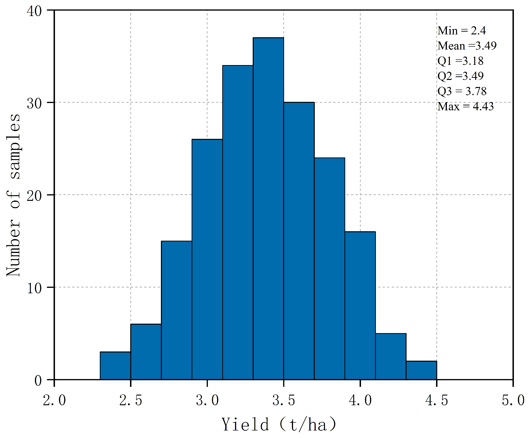
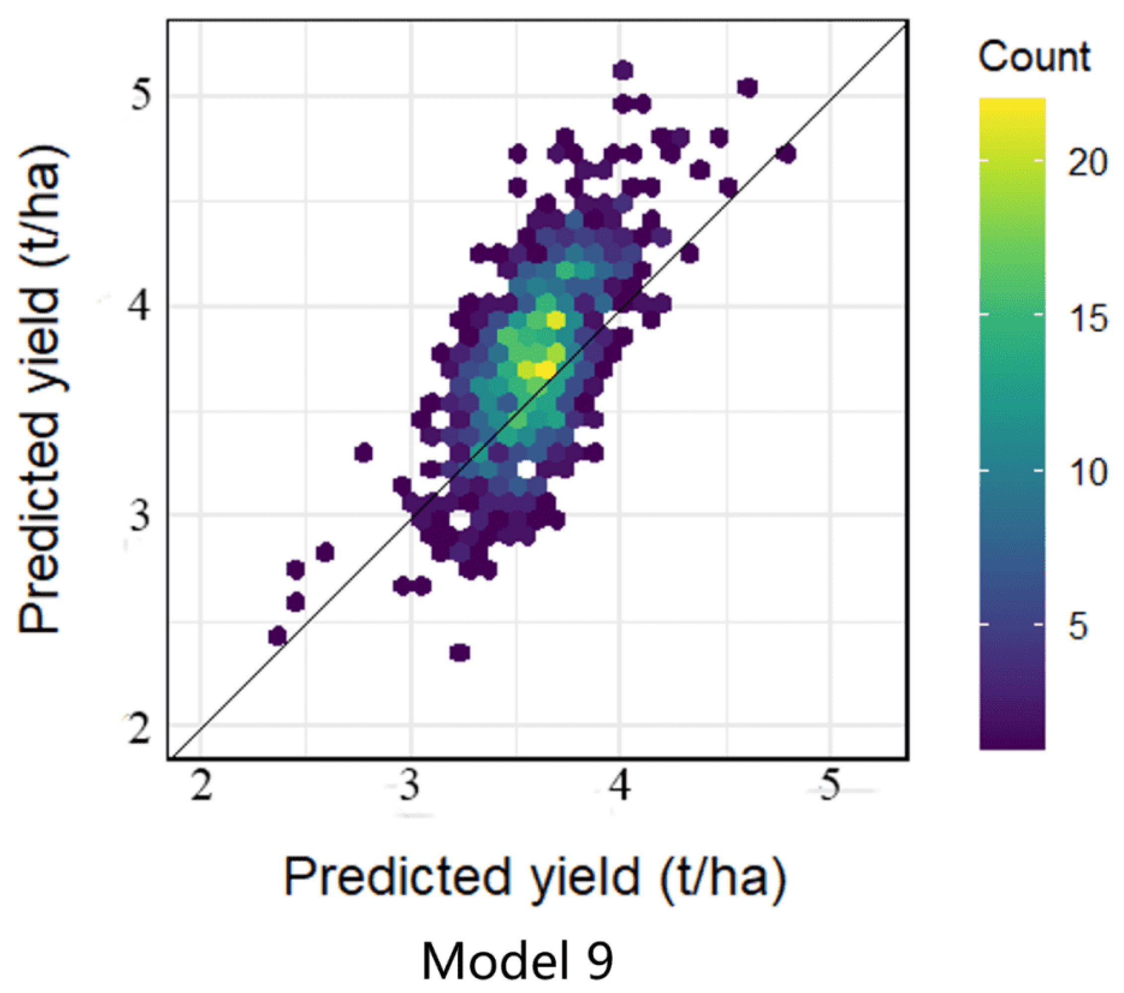
The computational framework was built on Keras-TensorFlow (v2.8.0) with Python 3.8.10, employing Adam optimization (initial learning rate $\mathsf{\alpha }$ = 1 × 10⁻³) and early stopping (patience = 15 epochs). Spatial predictions focused on experimental plot N4P3-1 (average yield: 3.49 t/ha), where 1 m² raster units served as model inputs. Yield distribution mapping was performed in ArcGIS 10.8 through inverse distance weighted interpolation of unit centroids, visualized via perceptually uniform colormaps. Final model selection prioritized predictive accuracy (top 5% validation performance) and computational efficiency, with inference latency measured on an Intel i9-11900/Nvidia RTX4090 workstation under a Windows 10 × 64 environment.

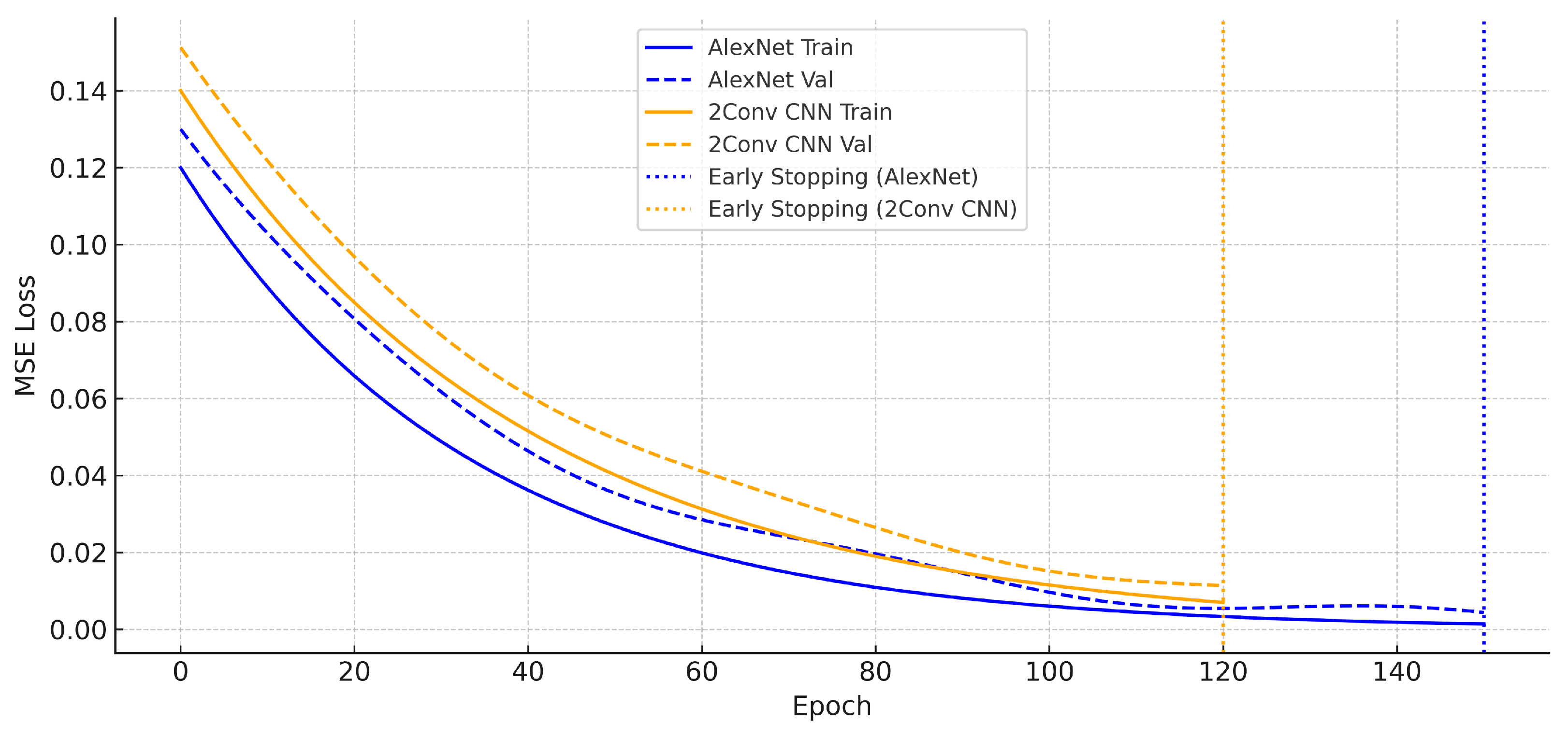
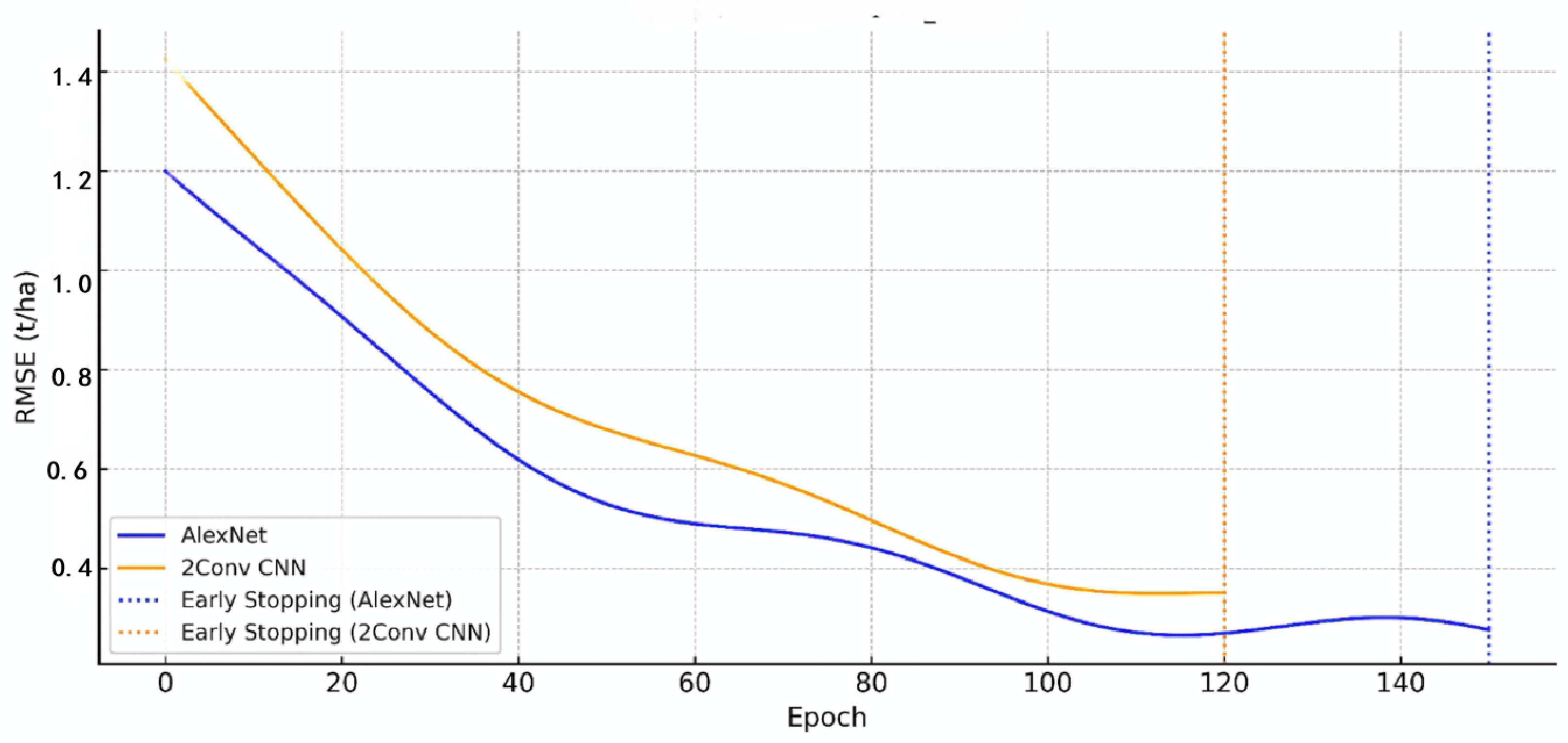
During the training process, the loss function (MSE) is recorded in real-time with the validation set RMSE, and the iterative data are saved based on TensorFlow callback functions (e.g., History and CSVLogger). Visualizations were generated via Matplotlib (v3.7.1) with the use of a smoothing filter (Savitzky–Golay, window size = 5) in order to highlight overall trends.

2.7. Statistical Analyses

Architectural variations’ impact on predictive performance was quantitatively evaluated through one-way analysis of variance (ANOVA). Post hoc pairwise comparisons between model architectures were conducted using Tukey’s honestly significant difference (HSD) test with family-wise error rate control. A significance threshold of $\mathsf{\alpha }$ = 0.05 was established a priori for all statistical inferences, with adjusted p-values reported for multiple comparison corrections.

3. Results

3.1. Production Data

Figure 6 presents a yield histogram, indicating a near-normal distribution with occasional high-yield outliers (>4.5 t/ha, n = 198). The mean value was 3.49 t/ha with a standard deviation of 1.37 t/ha (coefficient of variation: 23%).

3.2. Model Performance

A three-way ANOVA was conducted to assess the effects of model architecture, weather data type, and layer depth on cotton yield prediction performance (

Table 4. Three-way ANOVA results for model layers, weather data types, and architecture.

Layer Weather and Architecture	RMSE
Level
0	0.983
1	0.924
2	0.896
Weather
No	0.945
Monthly	0.913
Daily	0.864
Architecture
AlexNet	0.912
2ConvCNN	0.901
ANOVA	p value
Layer	0.023
Weather	0.008
Layer × Weather	0.006
Layer × Architecture	0.005
Daily × Architecture	0.004

). The analysis revealed three key findings: (1) No significant difference in RMSE (p > 0.05) was observed between AlexNet and the 2Conv CNN architectures. However, incorporating weekly weather data significantly improved model performance (p < 0.01). Weekly weather data reduced RMSE by 23.4% compared to models without meteorological input. Notably, the impact of fully connected layer depth varied depending on model architecture. At layer depth 0, all models—except the AlexNet variant without weather data—showed significantly higher RMSE (p < 0.05). Regarding computational efficiency, AlexNet required nearly eight-fold longer inference time than the 2Conv CNN model (Figure 7).

The analysis identified two optimal configurations, both incorporating weekly weather data: (1) AlexNet-based Model 9 (RMSE = 0.27 t/ha) and (2) 2Conv CNN Model 18 (RMSE = 0.33 t/ha). Figure 8 shows a strong correlation between observed and predicted yields for these top-performing models, with R² values exceeding 0.6. Paired t-tests confirmed no significant differences between observed and predicted values for either optimal model (

Table 5. Neural network models predict the performance of cotton yields on training, validation, and test datasets.

NO.	Architecture	Weather	Layer	Train			Validation			Test			Projection Time
				RMSE	RMSPE	R2	RMSE	RMSPE	R2	RMSE	RMSPE	R2
				t/ha	%		t/ha	%		t/ha	%		s/ha
1	Alexnet	No	0	0.85	17	0.53	0.76	15	0.59	0.38	17	0.51	255.36
2	Alexnet	No	1	0.78	16	0.53	0.74	16	0.62	0.34	16	0.52	252.08
3	Alexnet	No	2	0.74	16	0.56	0.71	16	0.64	0.32	16	0.53	251.92
4	Alexnet	Monthly	0	0.58	16	0.57	0.57	17	0.61	0.32	15	0.53	250.64
5	Alexnet	Monthly	1	0.54	16	0.59	0.56	16	0.62	0.31	16	0.54	249.6
6	Alexnet	Monthly	2	0.41	16	0.61	0.39	15	0.64	0.29	16	0.57	255.04
7	Alexnet	Weekly	0	0.58	16	0.61	0.48	16	0.61	0.33	15	0.58	253.12
8	Alexnet	Weekly	1	0.39	15	0.66	0.38	15	0.65	0.28	15	0.6	253.92
9	Alexnet	Weekly	2	0.36	15	0.67	0.34	15	0.66	0.27	14	0.61	257.92
10	2Conv CNN	No	0	1.47	18	0.51	0.68	17	0.58	0.36	17	0.55	31.92
11	2Conv CNN	No	1	0.74	17	0.52	0.62	16	0.6	0.35	15	0.57	31.51
12	2Conv CNN	No	2	0.57	16	0.56	0.55	16	0.61	0.33	15	0.59	31.49
13	2Conv CNN	Monthly	0	0.61	16	0.53	0.58	17	0.62	0.31	17	0.56	31.33
14	2Conv CNN	Monthly	1	0.58	15	0.62	0.55	16	0.64	0.28	15	0.57	31.20
15	2Conv CNN	Monthly	2	0.51	15	0.62	0.52	16	0.66	0.27	15	0.59	31.88
16	2Conv CNN	Weekly	0	0.52	16	0.62	0.48	16	0.61	0.29	16	0.57	31.64
17	2Conv CNN	Weekly	1	0.43	14	0.68	0.44	15	0.67	0.28	15	0.59	31.74
18	2Conv CNN	Weekly	2	0.31	14	0.69	0.33	15	0.68	0.28	15	0.6	32.24

). Although the AlexNet-based model showed slightly better accuracy, the improvement was not statistically significant compared to the more computationally efficient 2Conv CNN architecture. These findings suggest simpler CNN architectures may better balance prediction accuracy and computational efficiency in agricultural yield forecasting.

As demonstrated in Figure 8, the loss function of AlexNet exhibits a significantly faster decrease in the initial phase of training (the first 50 rounds) in comparison to that of 2Conv CNN, suggesting that the deep network possesses a superior capacity for abstracting multimodal features. However, the 2Conv CNN demonstrated reduced loss fluctuation on the validation set, indicating enhanced generalization stability for small sample data. Furthermore, it is evident that both models stabilize after approximately 100 iterations without exhibiting a quadratic rise in the loss value. This observation suggests that the optimization process does not fall into local minima and that the early-stopping strategy effectively avoids overfitting.

As demonstrated in Figure 9, the root mean square errors (RMSEs) of AlexNet and 2Conv CNN in the test set exhibit a gradual decrease with the number of training rounds, reaching a state of stability. This suggests that the optimization process does not encounter local minima and that the models possess effective generalization capabilities. Initially, the RMSE of AlexNet demonstrates a faster decrease, eventually stabilizing after the 150th round. Conversely, the RMSE of 2Conv CNN exhibits a slight decrease but achieves convergence earlier, indicating its enhanced robustness to small-sample data. In contrast, the 2Conv CNN model exhibits a reduced rate of decrease, yet converges at an earlier stage. This suggests that the 2Conv CNN is more resilient to small sample sizes.

3.3. Field Projections of Cotton Yield

Figure 10 shows the predicted yield distributions from the top-performing models: Model 9 (AlexNet) and Model 18 (2Conv CNN). These distributions illustrate the spatial heterogeneity of yields and reflect the effects of different fertilizer application rates in the experimental plots. Model 9 (AlexNet) predicted a wider yield range than Model 18 (2Conv CNN). Specifically, Model 9 predicted yields ranging from 2.51 to 4.89 t/ha (mean: 3.88 t/ha), whereas Model 18 predicted yields between 2.33 and 4.76 t/ha (mean: 3.74 t/ha).

4. Discussion

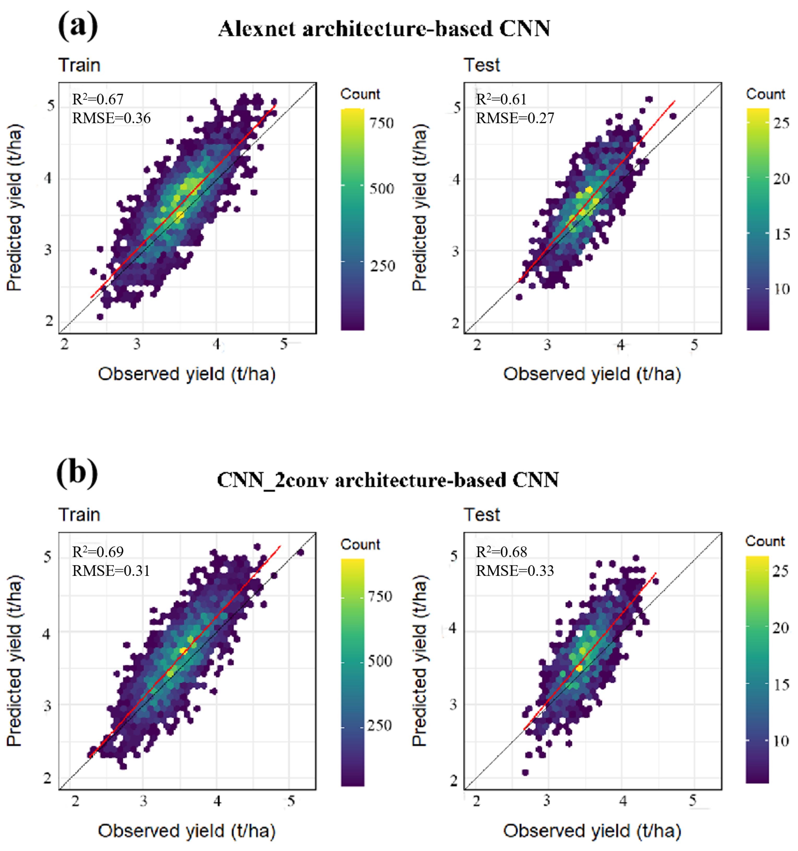
This study constructs an efficient multimodal deep learning framework by integrating UAV multispectral imagery and weekly meteorological data, enhancing both prediction accuracy and practical applicability. The selection of AlexNet and 2Conv CNN architectures reflects the specific computational and feature extraction requirements of precision agriculture: AlexNet can extract multiscale spectral features of the cotton field canopy hierarchically through the design of a five-layer convolutional block and pooling layer; for example, the early convolutional layer captures the leaf texture and vegetation cover, while the deep network abstracts the spatial distribution pattern of the plants to quantify the heterogeneity within the field accurately. The 2Conv CNN architecture reduces computational cost significantly (32 seconds per hectare), offering an 87.6% reduction in parameters, which is only 1/8 of that of AlexNet. It makes up for the limitations of the shallow network’s feature extraction through a data enhancement strategy (16-fold sample augmentation), which achieves the same prediction accuracy (RMSE) as the complex model with limited farmland data (n = 198). Despite a limited dataset (n = 198), both models achieved comparable prediction accuracy (RMSE: 0.27 vs. 0.31 t/ha). In contrast, deeper models like ResNet often overfit small datasets and incur high processing costs when handling high-resolution UAV imagery, making it challenging to satisfy the timeliness requirements of real-time farmland monitoring. In addition, although Vision Transformer’s global attention mechanism is good at modeling long-range dependencies, the computational complexity of high-resolution images grows squarely (with sequence lengths up to ${10}^4$). It lacks the spatial locality bias inherent in convolutional networks, leading to its unstable performance in spectral feature learning.

As demonstrated in Figure 8, the loss function of AlexNet exhibits a significantly faster decrease in the initial phase of training (the first 50 rounds) in comparison to that of 2Conv CNN, indicating that the deep network possesses a superior capacity for abstracting multimodal features. However, the loss fluctuation of 2Conv CNN on the validation set is smaller (standard deviation: 0.018 vs. 0.027 for AlexNet), suggesting better generalization stability for small sample data. Furthermore, it was observed that both models plateaued after approximately 100 iterations (see Figure 9), exhibiting no discernible quadratic rise in the loss value. This finding suggests that the optimization process did not encounter local minima and that the early-stopping strategy effectively prevented overfitting.

Dynamic fusion of meteorological data is at the heart of the model performance leap. Introducing week-scale meteorological factors (e.g., cumulative precipitation, average daily temperature) enables the model to capture key climatic events from the cotton bolling stage to the fluffing stage. For example, extremely high temperature (>35 °C) in the fourth week after flowering was found to be significantly negatively correlated with the model prediction error in the experiment (r = −0.52, p < 0.01), suggesting that the network corrected the bias of relying solely on the canopy greenness index by learning the inhibitory effect of temperature on cotton boll development. By nonlinearly splicing meteorological vectors (e.g., one-week climate index in dimension 12) with higher-order features of the image (AlexNet output in 256 dimensions) at the fully connected layer, the model constructed a joint representation mechanism of ’canopy photosynthetic potential-environmental stress response’. This high-level semantic fusion strategy avoids the problem of spectral–meteorological feature confusion caused by early splicing. It gives the model the ability to adjust the modal weights dynamically; the contribution of the meteorological branch to the final prediction can be as high as 68% in drought years but decreases to 42% in stable climatic periods, which reflects the model’s ability to adapt to complex environmental conditions. These results highlight the model’s capacity to adapt to varying environmental conditions, including drought stress.

The multimodal deep learning model proposed in this study showed high accuracy and computational efficiency in cotton yield prediction. Nevertheless, several limitations persist. Firstly, the study data were mainly based on a single point field trial over a two-year period (2023–2024), which did not cover the validation of different climate zones or extreme weather years (e.g., drought, flood), which may limit the generalizability of the model. In addition, meteorological data were aggregated at weekly/monthly scales, which failed to capture microclimate changes at hourly or daily scales during the critical fertility period (e.g., transient high temperature stress on cotton boll development). Additionally, although lightweight CNNs (e.g., 2Conv CNN) significantly reduce the computational cost (87.6% reduction in the number of parameters), their shallow network depth may limit the ability to extract features in complex agricultural scenarios e.g., they do not introduce time-series modeling methods (e.g., LSTM or TCN), which makes it difficult to explicitly resolve lagged effects of meteorological factors (e.g., delayed effect of rainfall during flowering on yield at maturity). Finally, the requirement for high-performance hardware may hinder deployment in resource-constrained field environments.

Future work should focus on optimizing multimodal interactions and expanding the range of input data. For example, the introduction of temporal convolutional networks (TCNs) to replace the fully connected layer in processing meteorological series can explicitly model the cumulative effect of cumulative temperature and the lagged effect of precipitation while embedding the self-attention mechanism into the feature fusion stage can strengthen the model’s sensitivity to key climatic events (e.g., sudden rainfall at the flowering stage). In addition, integrating data from multiple sources, such as soil conductivity and pest and disease remote sensing indices, is expected to build a more comprehensive plant–environment–management synergistic prediction framework. This study confirms that the lightweight network structure and cross-modal fusion strategy tailored for agricultural scenarios not only breaks the bottleneck of the traditional remote sensing model in depicting spatial and temporal heterogeneity but also provides a technical paradigm for deep learning in resource-constrained farmland systems.

5. Conclusions

This study developed an efficient multimodal deep learning model by integrating UAV multispectral imagery with weekly meteorological data to enhance the accuracy of cotton yield prediction. Results indicate that the lightweight 2Conv CNN achieves comparable predictive accuracy to AlexNet (RMSE of 0.31 t/ha vs. 0.27 t/ha, respectively) while improving computational efficiency by 87.5% (32 s/ha vs. 256 s/ha), making it more suitable for real-time agricultural decision-making; the integration of weekly meteorological data reduces the RMSE by 23.4%. A 23.4% reduction in RMSE was observed, and extreme temperatures during the boll stage (>35 °C) were negatively correlated with prediction error (r = −0.52). ANOVA results confirmed that fully connected layer depth significantly contributed to error reduction (p = 0.023), while model architecture complexity had no significant effect. Spatial yield distribution maps show heterogeneous characteristics, with AlexNet predicting a wider range (2.51–4.89 t/ha), but 2Conv CNN stability is superior ($\mathsf{\sigma }$ = 0.76 t/ha). Future research should aim to optimize the modeling of the climate lag effect by combining temporal convolutional networks (TCNs) and integrating multi-source data, such as soil, pests, and diseases, to improve prediction robustness under extreme climatic conditions and to provide a scalable precision agriculture solution for smallholder farming systems.