An Analysis of Uncertainties in Evaluating Future Climate Change Impacts on Cotton Production and Water Use in China

Abstract

Global Climate Models (GCMs) are a primary source of uncertainty in assessing climate change impacts on agricultural production, especially when relying on limited models. Considering China’s vast territory and diverse climates, this study utilized 22 GCMs and selected three representative cotton-producing regions: Aral (northwest inland region), Wangdu (Yellow River basin), and Changde (Yangtze River basin). Using the APSIM model, we simulated climate change effects on cotton yield, water consumption, uncertainties, and climatic factor contributions. Results showed significant variability driven by different GCMs, with uncertainty increasing over time and under radiation forcing. Spatial variations in uncertainty were observed: Wangdu exhibited the highest uncertainties in yield and phenology, while Changde had the greatest uncertainties in ET (evapotranspiration) and irrigation amount. Key factors affecting yield varied regionally—daily maximum temperature and precipitation dominated in Aral; precipitation was a major negative factor in Wangdu; and maximum temperature and solar radiation were critical in Changde. This study provides scientific support for developing climate change adaptation measures tailored to cotton production across different regions.

1. Introduction

1.1. Climate Projection Models and Their Uncertainties

Global Climate Models (GCMs) are tools used to project future climate changes based on historical climate observation data, capable of simulating climate variations across different spheres of the Earth. These climate projection models carry inherent uncertainties which manifest in several ways: (i) model structure and parameterization: these include limitations intrinsic to the model structure, parameterization schemes, assumptions, and calibration processes [1,2]; (ii) idealized conditions: the models are built under idealized conditions and thus struggle to accurately simulate the impacts of human activities, geographical locations, and atmospheric environments. Different GCMs exhibit varying performances across distinct regions [3]. In site-specific climate change projections, GCMs are employed to drive process-based models for assessing the effects of climate change [4,5]. However, discrepancies arise due to the varying temporal and spatial resolutions among different GCMs, leading to errors. Recent advancements in high-resolution regional modeling and downscaling techniques have significantly enhanced the ability to capture fine-scale climatic and environmental processes. Over the past five years, deep learning approaches have emerged as transformative tools for subgrid-scale parameterization and spatial downscaling [6,7]. These innovations highlight the shift toward physics-informed deep learning frameworks that combine high-resolution remote sensing inputs with computational efficiency. Ensemble methods further mitigate structural uncertainties by aggregating outputs from multiple General Circulation Models (GCMs) [8,9]. GCM selection and bias correction critically influence climate impact assessments, with ensemble mean projections often outperforming individual models [10]. Consequently, a common approach to reduce these errors and uncertainties in a given study area is to utilize an ensemble of multiple GCMs [2,11]. This ensemble method emphasizes the importance of integrating multiple models to enhance the reliability and accuracy of climate projections, thereby mitigating the uncertainties associated with individual models.

1.2. Application of Crop Models for Future Climate Impact Assessment

Crop models are extensively employed for assessing the impacts of future climate changes on crop production and formulating corresponding agricultural measures, offering a time-efficient and cost-effective approach. Integrating process-based crop models with climate models has been widely adopted by scholars globally. Due to variations in the applied crop models, climate models, and regional conditions, simulations of cotton yield and water consumption exhibit notable differences. For instance, Li et al. [12] conducted field experiments in central-eastern Texas, utilizing the APSIM model to simulate the impact of climate change on cotton yield and water use efficiency, revealing significant declines in both metrics under future climate scenarios. Luo et al. [13] simulated climate change and cotton water consumption across nine cotton-growing regions in eastern Australia using the CSIRO OZCOT model, indicating increased temperatures and precipitation, with irrigated cotton yields improving by 0–25% and water consumption rising by 0–4%. Chen et al. [14] combined the RZWQM2 model with six global climate models to predict the effects of climate change on cotton yield and water requirements in the Cele Oasis, Xinjiang, showing that lint cotton yields would increase by 5.6% and 4.5% under the RCP4.5 and RCP8.5 scenarios, respectively, during 2041–2060, while water requirements would decrease by 7.5% and 10.3%. Rahman et al. [15] used the CROPGRO-Cotton model to predict future climate impacts on cotton production in Pakistan, demonstrating mean seed cotton yield decreases of 12% and 30% under the RCP 8.5 scenario. In these studies focusing on cotton production projection within research areas, employing multiple climate models and scenarios is a common strategy to reduce errors and uncertainties. However, over 80% of studies focus on single regions, neglecting comparative analyses across agroecological zones [16].

1.3. Impacts of Climate Change on Cotton Growth and Water Consumption

Climate change exerts multifaceted impacts on cotton production through dynamic interactions between atmospheric, hydrological, and biological factors. The primary mechanisms manifest through two key drivers: temperature elevation and CO₂ concentration increase, with water availability serving as a critical mediating factor [17,18,19]. Rising temperatures accelerate cotton’s phenological development, compressing its growth cycle [20,21]. While this thermal acceleration might theoretically enhance growth rates, practical outcomes reveal significant trade-offs. Extreme heat events disrupt reproductive processes, inducing boll shedding and yield reduction through physiological stress [22,23,24]. Recent studies have highlighted the adverse effects of heatwaves on cotton production. Extreme temperatures during flowering and boll development stages significantly reduced fiber quality and yield [24,25]. Furthermore, heatwaves not only shorten the growing season but also increase the risk of premature shedding of cotton bolls, leading to lower productivity [18,26]. Concurrently, elevated temperatures amplify evapotranspiration demands [13], exacerbating water scarcity, particularly in arid production regions.

Elevated atmospheric CO₂ concentrations counteract thermal stresses through distinct physiological mechanisms. By enhancing ribulose-1,5-bisphosphate carboxylase/oxygenase (Rubisco) activity, CO₂ enrichment improves photosynthetic carbon assimilation rates while simultaneously reducing stomatal aperture and transpirational water loss [27,28]. This dual effect promotes dry matter accumulation in cotton plants, particularly under water-limited conditions, as demonstrated by a 12–18% increase in biomass production in free-air CO₂ enrichment (FACE) experiments [29]. However, the compensatory capacity of CO₂ fertilization is constrained by co-limiting factors: nutrient deficiencies (e.g., nitrogen) can reduce photosynthetic gains by 40–60%, while water scarcity thresholds determine whether CO₂-induced water savings translate to yield benefits [30,31]. Experimental evidence suggests that CO₂ enrichment may offset 10–30% of yield losses caused by moderate warming, but this mitigation potential diminishes under extreme heat (>35 °C) or prolonged drought, highlighting its context-dependent nature. Furthermore, the climatic effect is different, as shown by the research on a global scale [16,32,33]. For example, studies have found that irrigated cotton production benefits from CO₂ effects and is less vulnerable to climate change, whereas rainfed production in Africa and India shows higher sensitivity to varying climate conditions [16].

Process-based crop models reveal the emergent outcomes of interacting climate drivers, challenging single-factor predictions. The GOSSYM model simulations for Mississippi cotton systems demonstrated that CO₂ enrichment alone increased yields by 10% through enhanced photosynthesis, yet concurrent warming (+3 °C) and precipitation variability (−15%) reversed this gain, resulting in a net 9% yield decline [34]. Similarly, LPJmL model projections for 2050 showed that excluding CO₂ effects led to a 14% yield reduction from climate change, whereas incorporating CO₂ fertilization reversed this trend, projecting a 6% net increase [16]. These results are in agreement with multi-model syntheses indicating that CO₂ benefits dominate under moderate warming (+2 °C) but are negated by extreme heatwaves exceeding crop thermal thresholds [35,36]. Such findings underscore the necessity of integrating dynamic CO₂, temperature, and precipitation interactions, region-specific cultivar adaptations, and stochastic extreme event modules in predictive frameworks to avoid systematic underestimation of climate risks.

1.4. Objective of the Study

This study seeks to improve climate impact assessments of cotton production in China by addressing the existing gaps through three key approaches: First, we utilize 22 General Circulation Models (GCMs) of Coupled Model Intercomparison Project Phase 6 (CMIP6) across four Shared Socioeconomic Pathways (SSPs)—SSP1-2.6, SSP2-4.5, SSP3-7.0, and SSP5-8.5—to generate probabilistic projections that comprehensively capture the uncertainty space of future climate scenarios. This approach provides a robust foundation for understanding the range of potential climate impacts on cotton yields. Second, we focus on China’s three major cotton-producing regions—the northwest inland region, the Yellow River basin, and the Yangtze River basin—to identify region-specific vulnerabilities and adaptation needs. By analyzing these distinct agroecological zones, we aim to provide targeted insights for climate-resilient cotton production. Third, we quantify the relative contributions of key climatic factors—temperature, radiation, CO₂ concentration, and precipitation—to yield variability, offering a detailed understanding of the drivers of cotton productivity under changing climate conditions. Together, these advancements aim to inform sustainable agricultural practices and policy decisions in the face of climate uncertainty.

2. Materials and Methods

2.1. Study Area

The northwest inland region, Yellow River basin, and Yangtze River basin are China’s foremost cotton-growing regions. The northwest inland region, characterized by an arid climate with an annual precipitation of 15–380 mm, receives 2600–3400 h of annual sunshine, fostering significant day–night temperature variations. This supports a frost-free period of 170–230 days and accumulated temperatures ≥10 °C, ideal for drought-resistant cotton varieties. Average annual temperatures range from 7 °C to 14 °C. The Yellow River basin offers a more balanced climate, with 500–1000 mm of rainfall annually, ensuring a frost-free period of 180–230 days. Accumulated temperatures here support full cotton growth cycles, with mean annual temperatures of 12–15 °C and April-to-October averages of 19–22 °C. Annual sunshine is approximately 1900–2900 h, accommodating medium and early-maturing cotton types. The Yangtze River basin, distinguished by abundant annual rainfall (1000–1600 mm), provides a lengthy frost-free period of 227–278 days and high accumulated temperatures that are beneficial for rapid plant development. Annual temperatures range from 14 °C to 17 °C, averaging 22.5 °C during the main growing season (April to October). This region experiences 1200–2500 h of annual sunshine, supporting diverse, high-yielding, and quality cotton varieties. These three key regions demonstrate how varied climatic conditions can optimize cotton cultivation across China.

We selected three representative sites: Aral Station (Irrigation Experiment Station of the First Agricultural Division) for the northwest inland region, Wangdu Station (Baoding Irrigation Experiment Station) for the Yellow River basin, and Changde Station (National Meteorological Station) for the Yangtze River basin. The geographical locations of these study areas are shown in Figure 1.

Aral Station (40°33′ N, 81°16′ E, 1012.2 m a.s.l.) is located in the southern Xinjiang Uygur Autonomous Region, characterized by a warm temperate extreme continental arid desert climate with an average annual temperature of 11.4 °C and annual precipitation of 49 mm. The region experiences high evaporation and low precipitation, relying on irrigation from surrounding mountain glacier/snowmelt water. The soil is predominantly alluvial, with light sandy textures and significant salinization. Due to abundant sunlight and irrigation resources, the Xinjiang Cotton Region has become China’s primary long-staple cotton production base, accounting for over 90% of national cotton production in 2022.

Wangdu Station (38°41′ N, 115°08′ E, 40.09 m a.s.l.) is situated in Wangdu County, Hebei Province, within a piedmont plain depression at the terminus of an alluvial fan. It features a typical warm temperate semi-humid monsoon climate with an average annual temperature of 11.8 °C, wind speed of 2 m/s, precipitation of 507.5 mm, and 2580 annual sunshine hours. The growing season coincides with the periods of rain and heat. The brown loamy soil contains 1.24% organic matter, with available nitrogen (48.64 mg·kg⁻¹), phosphorus (17.46 mg·kg⁻¹), and potassium (95.05 mg·kg⁻¹). According to the China Statistical Yearbook (2023), Hebei Province had a cotton planting area of 116,100 hm² in 2022, representing 3.87% of the national total and ranking second only to Xinjiang.

Changde Station (29°03′ N, 111°41′ E, 35 m a.s.l.) lies in northwestern Hunan Province, a transitional central-to-north subtropical monsoon humid climate zone with plains, mountains, and hills. The region has an average annual temperature of 16.7 °C and annual rainfall of 1200–1900 mm. Cotton cultivation is concentrated in four northern counties (Anxiang, Lixian, Nan, and Huarong), covering approximately 64,600 hm² in 2022.

These three sites were selected for their high cotton yields and significant planting area proportions within their respective regions, making them representative of China’s three major cotton production zones.

2.2. Brief Introduction of APSIM-COTTON

APSIM (Agricultural Production Systems Simulator) is an agricultural production systems simulator developed by CSIRO (the Commonwealth Scientific and Industrial Research Organisation, Canberra, Australia) and APSRU (the Queensland Government’s Agricultural Production Systems Research Group, Queensland, Australia). The effects of climate, genotype, soil, and agricultural management practices on crop production can be modeled [37]. Since its establishment in 1996, the model has evolved from a planting system model to an agro-ecosystem model. APSIM provides a basic framework that includes biophysical modules, management modules, data input and output modules, and simulation engines that drive the simulation process and control all information exchanges between individual modules, allowing data to be exchanged between them. APSIM takes the soil module as the core and simulates crop growth and development through coupling with the crop module, which is its unique advantage over other crop models. APSIM has a strong ability to simulate the adjustment of crop planting structures, crop growth and development, yield prediction, and water resource management for different planting methods under various soil conditions in different climatic zones. As one of the models in the APSIM series, the APSIM-COTTON model is not only sensitive to yield changes and economic risks under extreme environmental conditions but can also simulate soil production potential under the influence of decision management practices such as cotton rotation and intercropping. The APSIM-COTTON, featuring a relatively simple mechanistic approach, enables precise assessment of the effects of climatic variations, soil conditions, and management practices on the present and projected productivity of cotton cultivation systems.

The APSIM-COTTON model mainly involves three modules: crop, soil, and management [12,38]. Among them, the crop module is mainly used to simulate cotton development and yield formation, including parameters related to crop varieties such as lint percentage, respiratory constant, leaf area growth rate, etc. The soil module primarily includes processes such as soil water balance and the transport and transformation of nitrogen, phosphorus, etc. The soil water module involves a series of processes such as precipitation, evapotranspiration, irrigation, runoff, and drainage. The management module facilitates user customization of variables, access to system-defined parameters, and redefinition of the simulation process in accordance with specific agricultural production scenarios. Key components of this module encompass sowing, irrigation, fertilization, harvesting, and other essential management practices.

The model setup used mainly for sowing and irrigation rules is outlined as follows: A 5-day running mean temperature exceeding 10 °C was used to indicate the time to start sowing, because it resulted in the lowest probability of low temperatures halting crop growth after emergence. Irrigation was set at 100 mm before sowing, and automatic irrigation occurred subsequently, except within 40 days of sowing (during seedling) and less than 10 days after the first boll opening. Automatic irrigation was triggered when the fraction of available soil water fell to 0.5 and finished when it reached 1.0. The wetting depth was set to 60 cm. At sowing, 150 kg N/ha was applied as urea and 50 kg N/ha was applied during every subsequent irrigation. To stabilize the effect of water and fertilizer application on the simulation results, the same rules for irrigation and fertilizer application were used in the baseline and future scenarios.

2.3. Data Resources

2.3.1. Meteorological Data

Historical climate data, including daily precipitation (mm), sunshine duration (hours), maximum temperature (°C), minimum temperature (°C), and other meteorological indices from 1961 to 2012, were obtained from the China Meteorological Science Data Sharing Service Network (CMDSSS) (https://data.cma.cn/data/, accessed on 1 January 2013). Sunshine duration data were subsequently converted into solar radiation (MJ·m⁻²) using the method proposed by Brock [39]. Historical data from the three national standard meteorological stations—Aral Station (ID: 51730, 40°33′ N, 115°08′ E, 1012.2 m a.s.l.), Wangdu Station (ID: 54607, 38°41′ N, 115°08′ E, 40.09 m a.s.l.), and Changde Station (ID: 57662, 29°03′ N, 111°41′ E, 35 m a.s.l.)—were employed to downscale GCM (Global Climate Model) outputs.

For future climate projections, data from the Coupled Model Intercomparison Project Phase 6 (CMIP6) dataset, encompassing 22 Global Climate Models (GCMs), were utilized (available at https://aims2.llnl.gov/search/, accessed on 1 January 2019).

Table 1. Information of the 22 Global Climate Models (GCMs) applied in the study.

Number	Code	Name	Institution	Country	Spatial Resolution (°)
1	ACC1	ACCESS-CM2	CSIRO-ARCCSS-BoM	Australia	1.2 × 1.8
2	ACC2	ACCESS-ESM1-5	CSIRO	Australia	1.2 × 1.8
3	BCC	BCC-CSM2-MR	BCC	China	1.1 × 1.1
4	Can1	CanESM5	CCCMA	Canada	2.8 × 2.8
5	Can2	CanESM5-CanOE	CCCMA	Canada	2.8 × 2.8
6	CNR1	CNRM-ESM2-1	CNRM-CERFACS	France	1.4 × 1.4
7	CNR2	CNRM-CM6-1	CNRM-CERFACS	France	1.4 × 1.4
8	CNR3	CNRM-CM6-1-HR	CNRM-CERFACS	France	0.5 × 0.5
9	ECE1	EC-Earth3-Veg	EC-Earth-Consortium	EU	0.7 × 0.7
10	ECE2	EC-Earth3	EC-Earth-Consortium	EU	0.7 × 0.7
11	FGOA	FGOALS-g3	CAS	China	2.3 × 2.0
12	GFD	GFDL-ESM4	NOAA-GFDL	US	1.0 × 1.3
13	GISS	GISS-E2-1-G	NASA-GISS	US	2.0 × 2.5
14	INM1	INM-CM4-8	INM	Russia	1.5 × 2.0
15	INM2	INM-CM5-0	INM	Russia	1.5 × 2.0
16	LPSL	IPSL-CM6A-LR	LPSL	France	1.3 × 2.5
17	MIR1	MIROC6	MIROC	Japan	1.4 × 1.4
18	MIR2	MIROC-ES2L	MIROC	Japan	2.7 × 2.8
19	MPI1	MPI-ESM1-2-HR	MPI-M	Germany	0.9 × 0.9
20	MPI2	MPI-ESM1-2-LR	MPI-M	Germany	1.9 × 1.9
21	MTIE	MRI-ESM2-0	MIR	Japan	1.1 × 1.1
22	UKES	UKESM1-0-LL	MOHC	UK	1.3 × 1.9

provides detailed information on these GCMs. This study selected four representative climate scenarios from the GCMs based on the Intergovernmental Panel on Climate Change (IPCC) Special Report on Emissions Scenarios: SSP5-8.5 (high-emissions scenario), SSP3-7.0 (high-emissions scenario), SSP2-4.5 (medium-emissions scenario), and SSP1-2.6 (low-emissions scenario).

The GCM data were downscaled by Deli Liu, a researcher at the Wagga Wagga Agricultural Research Institute, Department of Primary Industries (DPI), Australia. This downscaled dataset employs the NWAI-WG statistical downscaling method [40]. Through this method, data from three stations were spatially and temporally downscaled to generate daily station climate data. Initially, the monthly General Circulation Model (GCM) data were downscaled to site-specific monthly data by integrating spatial interpolation with bias correction techniques, calibrated against observational data spanning from 1961 to 2010. Subsequently, the refined site-specific monthly data were disaggregated into daily data using an enhanced version of the WGEN weather generator [41]. The downscaled GCM (Global Climate Model) outputs were formatted according to the APSIM meteorological data specifications to generate text files compatible with crop model operations.

2.3.2. Soil Data

The physical properties of a continuous soil layer are characterized by a set of parameters, including bulk density (g cm⁻³), air-dry water content (mm mm⁻¹), wilting point (mm mm⁻¹), field capacity (mm mm⁻¹), saturated water content (mm mm⁻¹), pH value, and soil particle composition. With the exception of the wilting point—estimated by the crop model—all other soil parameters were determined experimentally through a sampling approach. Soil profiles were analyzed across a 2 m depth, with increments of 15 cm for the 0–30 cm layer and 30 cm for the 30–200 cm layer in Aral and Wangdu.

For Changde, bulk density and particle size distribution data were obtained from a representative section of China’s national soil database (https://soil.geodata.cn/, accessed on 1 January 2024). Other pertinent soil parameters were estimated using the SPAW model [42], based on bulk density and particle size distribution. Detailed parameter values are provided in

Table 2. Soil parameters in the profiles.

	Depth	Bulk Density	Air-Dry Water Content	Wilting Point	Field Capacity	Saturated Water Content
	cm	g·cm−3	mm·mm−1	mm·mm−1	mm·mm−1	mm·mm−1
Aral	0–15	1.200	0.060	0.080	0.280	0.350
	15–30	1.200	0.060	0.120	0.300	0.380
	30–60	1.400	0.060	0.150	0.320	0.410
	60–90	1.490	0.060	0.080	0.280	0.350
	90–120	1.560	0.060	0.080	0.280	0.350
	120–150	1.470	0.060	0.080	0.280	0.350
	150–180	1.470	0.060	0.080	0.280	0.350
Wangdu	0–15	1.470	0.060	0.119	0.274	0.425
	15–30	1.460	0.059	0.119	0.273	0.448
	30–60	1.390	0.050	0.109	0.264	0.444
	60–90	1.510	0.060	0.109	0.274	0.430
	90–120	1.510	0.058	0.097	0.272	0.430
	120–150	1.553	0.055	0.097	0.269	0.414
	150–180	1.510	0.065	0.097	0.313	0.430
Changde	0–12	1.470	0.050	0.090	0.365	0.445
	12–25	1.480	0.059	0.090	0.365	0.442
	25–65	1.490	0.060	0.115	0.300	0.410
	65–100	1.510	0.062	0.115	0.290	0.400

.

2.3.3. Crop Data

To enhance the applicability of the APSIM-COTTON model for localization studies in Aral, Wangdu, and Changde, model parameters were calibrated and validated using our field experimental data collected from Aral in 2011 and 2012 and Wangdu in 2019 and 2020. The experiment was designed based on the conventional agricultural practices of local farmers, adhering to their preferred time of sowing and harvesting, row spacing, irrigation, fertilization, etc. The observation items included the phenology, morphology (e.g., LAI, plant height, number of leaves, squares, bolls, etc.), yield, and dry matter distribution, as well as soil moisture characteristic parameters and soil moisture dynamics. For detailed experimental setups and parameter calibration procedures, please refer to Yang et al. [38] and Wang et al. [43].

The validation results from Aral are shown in Figures S1 and S2 and Table S1 in the Supplementary Materials. The key crop growth indicators included the leaf area index (LAI), square number, green bolls number, open bolls number, and dry matter weight of biomass. The determination coefficient (R²) value for the open bolls number was higher than those for the square number and bolls number. The R² values for all parts exceeded 0.7, with normalized root mean square errors (NRMSEs) ranging between 0.2 and 0.4085, indicating reliable morphological simulations in Aral. Figure S2 also demonstrates the goodness of fit between the simulated and observed dry matter of different plant parts in Aral. Except for the dry matter weight of leaves, the R² values of stem, bolls, etc., exceeded 0.8, confirming strong agreement between the model simulation and field observations.

The validation results in Wangdu are shown in Figures S3 and S4 and Table S2. The R² between simulated and observed values ranged from 0.70 to 0.99 (excluding green bolls number), while the NRMSE ranged from 0.21 to 2.24. The simulated lint cotton yield was 1125.1 kg·hm⁻², while the observed one was 1397.8 kg·hm⁻². The close agreement between the simulated and experimental values demonstrates the model’s reliability in simulating cotton production.

For Changde, calibration was conducted based on aggregated statistical data and literature-derived information. The selection of cultivar-specific parameters and agricultural management practices primarily relied on field trial results and local cotton farmers’ established practices while acknowledging potential limitations in broader representativeness. The calibrated model parameters for the three locations are summarized in

Table 3. Cotton variety parameters for the three sites for APSIM-COTTON.

Parameter	Unit	Description	Wangdu	Aral	Changde
	Percent_l	Percent of lint	43	41	36
Scboll	g/Boll	Seed cotton per boll	3.8	5.5	5
Respcon		Respiration constant	0.01593	0.02500	0.02306
Sqcon		Rate of squaring in thermal time	0.0181	0.021	0.0116
Fcutout		Constant relating timing of cutout to boll load	0.5411	0.4789	0.4789
Flai		Ratio of leaf area per site	0.52	0.87	0.87
DDISQ	°C·d	Thermal time between emergence and the first square	402	380	450
TIPOUT		Tipping out time	52	75	52
FRUDD(8)	°C·d	Thermal time for each cotton fruiting stage	50, 169, 329, 356, 499, 642, 857, 1099	50, 180, 380, 400, 570, 630, 900, 1115	50, 250, 330, 420, 512, 610, 820, 1050
BLTME(8)		Fraction of boll development in one day	0, 0, 0, 0.07, 0.21, 0.33, 0.55, 1	0, 0, 0, 0.07, 0.21, 0.33, 0.55, 1	0, 0, 0, 0.07, 0.21, 0.33, 0.55, 1
Dlds_max		Maximum LAI growth rate	0.12	0.10	0.23
Rate_emergence		Rate of emergence	1	1	1.2
Popcon		Plant population constant	0.03633	0.3633	0.03633
Fburr		Ratio of seed cotton to seed cotton and burr per boll	1.23	1.23	1.73
ACOTYL	mm2	Area of cotyledons	525	525	525
RLAI		Growth rate of leaf area with water stress before squaring	0.01	0.01	0.01

.

2.4. Statistical Method

2.4.1. Multiple Linear Regression

Multiple linear regression (MLR) was employed to analyze the relationship between cotton yield and factors including solar radiation, minimum temperature, maximum temperature, precipitation, and CO₂ concentration over the period of 1961–2100. The MLR equation used in this study is formulated as follows:

$$Y_c=aR+b{T}_{min}+c{T}_{max}+dP+eC$$

(1)

where Yc represents cotton yield (kg ha⁻¹), and R, T_min, T_max, P, and C denote the normalized values of solar radiation (MJ m⁻²), minimum temperature (°C), maximum temperature (°C), rainfall (mm), and CO₂ concentration (mmol L⁻¹) during the growth period, respectively. The coefficients a, b, c, d, and e represent the regression coefficients for each corresponding variable.

2.4.2. Contribution Percentage

The contribution percentage of each meteorological factor—solar radiation, minimum temperature, maximum temperature, precipitation, and CO₂ concentration—to cotton yield was quantified based on the regression coefficients obtained from the multiple regression equation. The contribution rate was calculated using the following formula:

$$n_1={\displaystyle \frac{\left|a\right|}{\left|a\right|+\left|b\right|+\left|c\right|+\left|d\right|+\left|e\right|}}$$

$$n_2={\displaystyle \frac{\left|b\right|}{\left|a\right|+\left|b\right|+\left|c\right|+\left|d\right|+\left|e\right|}}$$

$$n_5={\displaystyle \frac{\left|e\right|}{\left|a\right|+\left|b\right|+\left|c\right|+\left|d\right|+\left|e\right|}}$$

(2)

where $n_1{,n}_2{,\dots n}_5$ refer to the contribution percentage of R, $T_{min}$, $T_{max}$, $P$, $C$, and $Y_c$.

3. Results

3.1. Evaluation of GCMs After Statistical Downscaling

The Taylor diagrams provided assess the performance of various models in simulating three meteorological factors—radiation, precipitation, and temperature—at three different locations: Aral, Wangdu, and Changde (Figure 2). The analysis reveals distinct patterns in model performance across these factors and locations.

In Aral, the correlation coefficients (CCs) between simulated and observed temperatures exceeded 0.9 for the models BCC, Can2, INM1, MITE, and UKES. Meanwhile, the normalized standard deviations (Norm SDs) for ACC2, BCC, Can1, Can2, CNR1, INM1, and MTIE were below 0.3. Overall, the four models—BCC, Can2, INM1, and MTIE—demonstrated the strongest performance in simulating temperatures in Aral. For precipitation, the CNR3 model exhibited a significantly higher CC compared to other models, which generally fell below 0.8. When evaluating solar radiation, the majority of models produced lower CCs (only FGOA and MPI1 exceeded 0.80) between simulated and observed values compared to temperature and precipitation.

In Wangdu, the Can2 model significantly outperformed other models in temperature simulations, achieving a CC of 0.93 and Norm SD of 0.01. For solar radiation in Wangdu, the CNR2 and ECE1 models demonstrated strong performance, with CCs exceeding 0.9, while the BCC and CNR3 models exhibited lower CCs of 0.78 and 0.75, respectively. Other models showed only moderate accuracy in replicating observed solar radiation patterns in Wangdu. Turning to precipitation in Wangdu, the ACC1, ACC2, and IPSL models achieved CCs greater than 0.9, with ACC2 and IPSL further distinguished by low Norm SD values of 0.13 and 0.28, respectively, underscoring their superior performance in simulating precipitation in this region. Overall, the evaluation of the 22 GCMs revealed notable variability in their ability to accurately model temperature, solar radiation, and precipitation specifically for Wangdu.

In Changde, regarding temperature, the GFD2, INM1, and INM2 models achieved a CC exceeding 0.9 and a Norm SD below 0.3, indicating their strong performance in temperature simulations. For solar radiation, both the BCC and INM2 models demonstrated CCs greater than 0.9 and Norm SDs below 0.2, showcasing robust accuracy in replicating observed solar radiation patterns. In contrast, precipitation simulations revealed mixed results: while the ACC2, BCC, and MIR1 models achieved relatively high CCs, their Norm SDs were notably larger, suggesting reduced precision. Overall, the INM2 model emerged as the top performer in Changde, consistently delivering high CCs and low Norm SDs across temperature and solar radiation metrics.

3.2. Change of Climate for the Three Sites

For daily maximum air temperature (Tmax), under the lower radiative forcing scenarios (SSP1-2.6 and SSP2-4.5), Changde exhibited the largest increase (5.97% to 14.55%), followed by Aral (6.16% to 14.13%), while Wangdu showed the smallest increase (5.43% to 13.21%). Under the higher radiative forcing scenarios (SSP3-7.0 and SSP5-8.5), the percentage increase for Aral was the highest (6.12% to 26.25%), followed by that for Changde (5.04% to 25.41%), with Wangdu recording the smallest increase (4.23% to 22.45%). The detailed results can be found in Table S1 of the Supplementary Materials.

For daily minimum air temperature (T_min), the percentage increase at all three stations was greater than that for T_max. Among them, Aral experienced the most significant increase (30.21% to 129.48%), followed by Wangdu (18.28% to 70.43%), while Changde had the smallest increase (8.22% to 33.87%). The detailed results can be found in Table S1 of the Supplementary Materials.

Regarding solar radiation, the Aral region exhibited a decreasing trend across most scenarios, with variations ranging from −0.23% to −4.56%. Conversely, both the Wangdu and Changde regions showed an increasing trend in solar radiation, except under the SSP3-7.0 scenario. Notably, the percentage increase in solar radiation was more pronounced in Changde (1.69% to 13.75%) compared to Wangdu (0.39% to 9.56%). The detailed results can be found in Table S2 of the Supplementary Materials.

With respect to precipitation, projections indicated an overall increase at all stations. Among these, Changde was projected to experience the smallest increase in precipitation, with a range of 3.18% to 21.50%. For Wangdu, the precipitation across all scenarios for the 2030s and throughout the periods under the SSP1-2.6 scenario was expected to surpass that of Aral. However, in the other three scenarios, excluding the 2030s, the percentage increase in precipitation in Wangdu (22.14% to 50.79%) was generally smaller than that in Aral (26.91% to 46.06%). The detailed results can be found in Table S2 of the Supplementary Materials.

3.3. Change of the Phenology and Uncertainty

The sowing dates at the three sites were observed to occur earlier compared to the baseline period, with advancements ranging from 1.7 to 16.8 days in Aral, 0.9 to 14.7 days in Wangdu, and 3.8 to 10.7 days in Changde (Figure 3). This trend towards earlier sowing was more pronounced with increasing radiative forcing and time progressing. Uncertainty caused by different GCMs also escalated with higher levels of radiative forcing and time passing. However, the response varied by location:

(1) For Aral, minimal inter-period differences were noted under the lower radiative forcing scenarios (SSP1-2.6 and SSP2-4.5). Conversely, under higher forcing scenarios (SSP3-7.0 and SSP5-8.5), the mean reduction in sowing days and variation (uncertainty) among different GCMs for the 2070s and 2090s was considerably greater than for the 2030s and 2050s. (2) In Wangdu, the mean sowing date and variation in the 2030s showed little deviation from the baseline year. However, the changing magnitude of the sowing date increased progressively with each subsequent two-decade period in SSP2-4.5, SSP3-7.0, and SSP5-8.5. The uncertainty increased with time passing in SSP5-8.5, but the same trend was not found in other scenarios. However, in all scenarios, the uncertainty in the 2090s was greater than in the other periods. (3) In Changde, the sowing day was significantly earlier than that in baseline in all scenarios and periods. The inter-period variations in the future were obvious in most scenarios except SSP1-2.6. The uncertainty in the 2050s and 2070s (especially for the 50% interquartile range) was greater than in other periods in most scenarios (except SSP2-4.5).

The analysis of uncertainty among the three sites indicates that the variations in Wangdu and Changde were greater than in Aral in most periods and scenarios. However, in the 2090s of SSP3-7.0 and SSP5-8.5, Aral was greater than Wangdu and Changde.

For the boll opening day, all three sites experienced an earlier onset compared to the baseline year, with the greatest advancement observed in Aral, followed by Wangdu, and the least in Changde. Under the SSP1-2.6 scenario, the mean differences in the boll opening stage across the four two-decade periods were minimal. However, under the other three scenarios (SSP2-4.5, SSP3-7.0, and SSP5-8.5), the advancement in the boll opening date increased with both the passage of time and the increase in radiative forcing. The uncertainty in the boll opening day generally increased from 2030 to 2090, especially under higher-emissions scenarios (SSP5-8.5). Aral showed higher uncertainty compared to Wangdu and Changde.

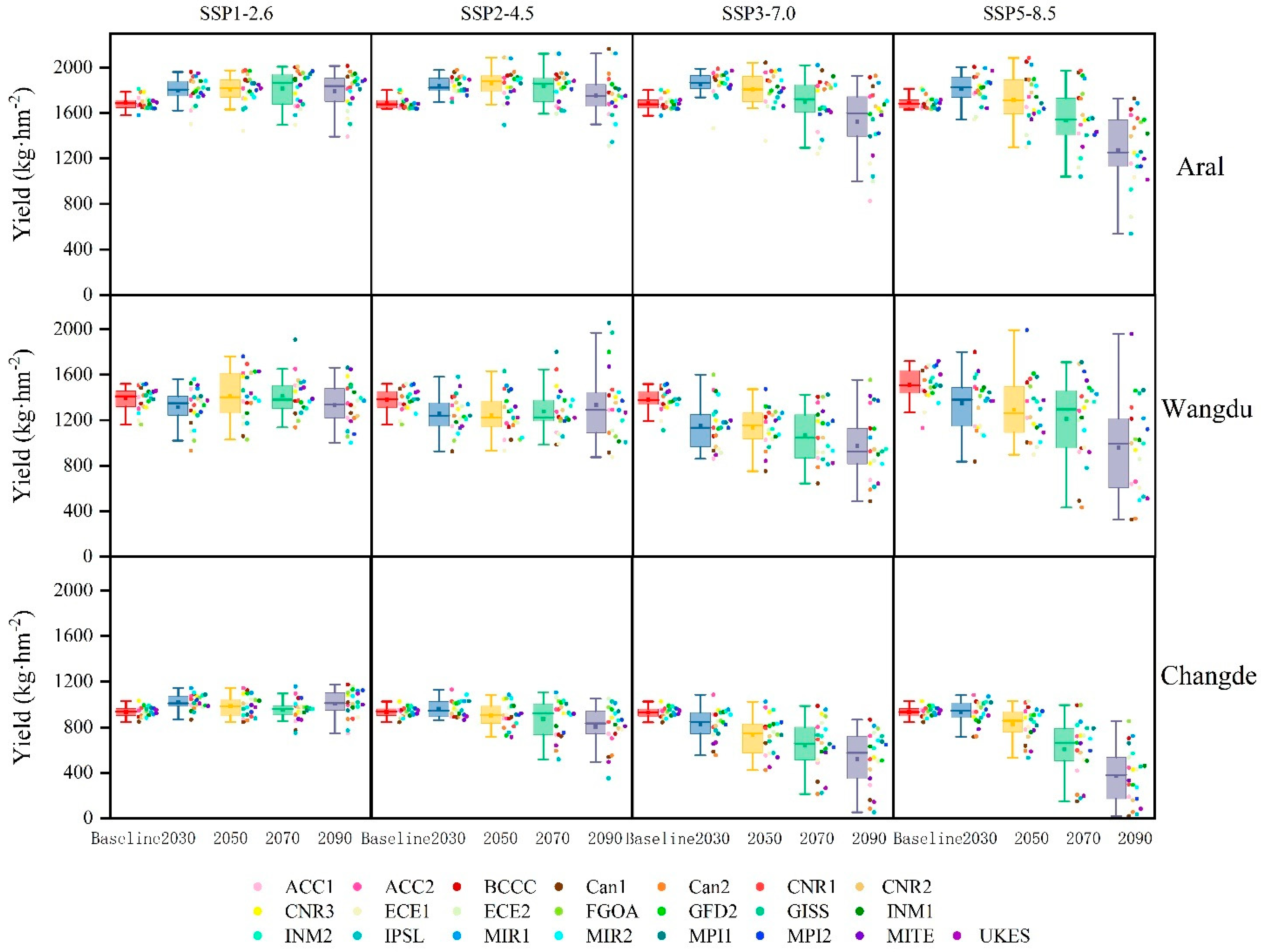
3.4. Change of the Yield and Uncertainty

In Aral, the yield under the SSP1-2.6 and SSP2-4.5 scenarios showed an increase of 3% to 10.6% compared to the baseline period (1690.7 kg·hm⁻²) (Figure 4). Under the higher radiative forcing scenarios SSP3-7.0 and SSP5-8.5, the yield initially increased before decreasing, leading to reductions of 11.6% and 24.5%, respectively, by the 2090s.

In Wangdu and Changde, cotton yields exhibited minimal differences across decades under the low radiative forcing scenarios (SSP1-2.6 and SSP2-4.5) (Figure 4). However, under high radiative forcing scenarios, there was a trend towards reduced yields. Specifically, under the SSP5-8.5 scenario, by the 2090s, yields decreased by 432.5 kg·hm⁻² in Wangdu and 562.2 kg·hm⁻² in Changde relative to their respective baseline periods (1392.3 kg·hm⁻² and 936.1 kg·hm⁻²). The uncertainty in yield predictions generally increased from the baseline to 2090, especially under higher-emissions scenarios (SSP5-8.5). Wangdu showed the greatest uncertainty, followed by Aral and Changde. Certain models (e.g., CNR1, CNR2) consistently showed higher uncertainty across all sites and scenarios.

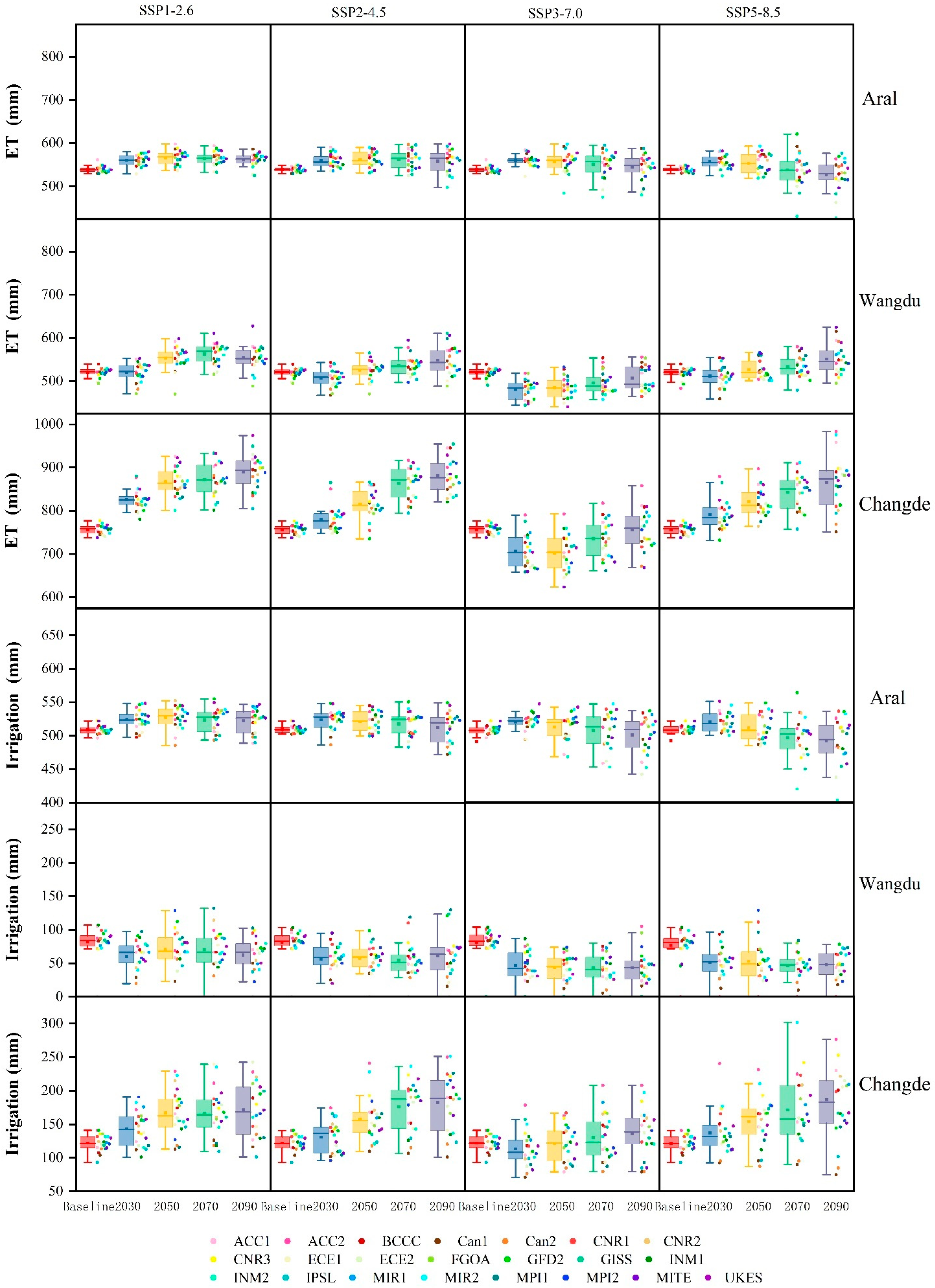
3.5. Change of the Water Use and Uncertainty

In Aral, the rate of ET in the future was slightly higher than at the baseline in most scenarios, and there was little difference or a slight decrease over time (Figure 5). However, in Wangdu, the ET increased with time in most scenarios, and the ET projections were all greater than that at the baseline, except in SSP3-7.0. In Changde, the increasing trend was more obvious, except in SSP3-7.0, in which the ET projection was less than the baseline. Among the three sites, Changde exhibited the highest uncertainty in the GCMs, followed by Wangdu, while Aral showed the least.

The irrigation amount in Aral in most future scenarios was greater than at the baseline, except in SSP5-8.5, and decreased with time. In Wangdu, it was less than at the baseline and the difference among the future periods was small. However, there was an increasing trend in Changde and the difference among periods was larger than that in Aral and Wangdu. The uncertainty of the GCMs was greatest in Changde, followed by Wangdu, and smallest in Aral.

3.6. Contribution of Climatic Factors to Cotton Yield

Through correlation analysis of 4400 simulation results from 100 years, 22 GCMs, and 4 scenarios at each site, the relationships between cotton yield and five major climate factors were determined (

Table 4. Coefficients of multiple linear regression analysis of cotton yield and climatic factors in Aral, Wangdu, and Changde.

	Scenario	Radiation	Max T	Min T	Precipitation	[CO2]	R2
	SSP1-2.6	0.12 ***	−0.2 ***	0.04	0.2 ***	0.19 ***	0.76
	SSP2-4.5	0.04 **	−0.18 ***	0.18 ***	0.03	0.09 ***	0.74
Aral	SSP3-7.0	0.07 ***	−0.42 ***	0.37 ***	0.005	−0.02	0.67
	SSP5-8.5	0.1 ***	−6.47	−4.73	10.73	−0.15 ***	0.56
	All	0.09 ***	−0.32 ***	0.45 ***	0.15 ***	−0.19 ***	0.71
	SSP1-2.6	0.23 ***	−0.21 ***	0.22 ***	−0.94 ***	0.02	0.61
	SSP2-4.5	0.22 **	−0.16 **	0.12 **	−0.87 ***	0.03	0.55
Wangdu	SSP3-7.0	0.15 ***	0.02	−0.08	−0.8 ***	0.003	0.46
	SSP5-8.5	0.13 ***	−0.02	−0.11 *	−1.04 ***	0.04	0.48
	All	0.21 ***	−0.10 ***	0.11 ***	−1.11 ***	−0.03	0.57
	SSP1-2.6	0.37 ***	−0.24 ***	0.15 ***	−0.27 ***	0.003	0.49
	SSP2-4.5	0.41 ***	−0.54 ***	0.05	−0.31 ***	0.04 *	0.51
Changde	SSP3-7.0	0.42 ***	−0.73 ***	−0.11	−0.42 ***	0.08 **	0.48
	SSP5-8.5	0.49 ***	−0.84 ***	0.01	−0.26 ***	−0.15 ***	0.45
	All	0.51 ***	−0.71 ***	0.19 ***	−0.27 ***	−0.22 ***	0.43

Note: Significance levels are denoted as follows: *** indicates p < 0.001, ** indicates p < 0.01, and * indicates p < 0.05.

). Generally, across all sites, cotton yield showed a significant positive correlation with solar radiation and a negative correlation with maximum daily temperature. The relationship with minimum daily temperature was positive under most scenarios, and especially in the low radiative forcing scenarios. The relationship with precipitation varied by site: it was positively correlated in Aral and negatively correlated in Wangdu and Changde. Cotton yield was positively correlated with CO₂ concentration in most scenarios, except for in Aral under the SSP3-7.0 and SSP5-8.5 scenarios, and in Changde under the SSP5-8.5 scenario, where a negative correlation was observed. In terms of the R² values of the regression equations under different scenarios, as radiative forcing increases, leading to greater weather variability and higher uncertainty, there is a tendency for R² to decrease. Among different locations, the R² value was highest in Alar, followed by Wangdu, and lowest in Changde.

The contribution of different climatic factors to cotton yield varied across regions (

Table 5. Contribution of climatic factors to the cotton yield in Aral, Wangdu, and Changde.

	Scenario	Radiation	Max T	Min T	Precipitation	[CO2]
Aral	SSP1-2.6	16.57%	26.14%	5.26%	26.52%	25.51%
	SSP2-4.5	7.88%	34.97%	34.71%	5.86%	16.57%
	SSP3-7.0	8.37%	47.28%	41.94%	0.54%	1.87%
	SSP5-8.5	0.46%	29.17%	21.31%	48.39%	0.67%
Wangdu	SSP1-2.6	14.35%	12.94%	13.54%	58.02%	1.15%
	SSP2-4.5	15.49%	11.45%	8.79%	61.96%	2.30%
	SSP3-7.0	14.43%	1.60%	7.24%	76.38%	0.35%
	SSP5-8.5	9.95%	1.60%	8.33%	77.23%	2.88%
Changde	SSP1-2.6	35.56%	22.82%	15.03%	26.30%	0.29%
	SSP2-4.5	30.13%	41.46%	3.91%	22.97%	2.97%
	SSP3-7.0	23.99%	41.46%	6.13%	24.07%	4.35%
	SSP5-8.5	27.95%	47.97%	0.76%	15.00%	8.31%

). In Aral, the daily maximum temperature, daily minimum temperature, and precipitation were the most significant contributors to yield. Under the SSP2-4.5 and SSP3-7.0 scenarios, the maximum and minimum temperatures had the greatest impact on cotton yield in Aral, with the maximum temperature exerting a negative influence of −34.97% and −47.28%, respectively, while the minimum temperature had a positive effect of 34.71% and 41.94%. Under the SSP1-2.6 and SSP5-8.5 scenarios, the precipitation during the growing season became the most influential factor, contributing 26.52% and 48.39%, respectively.

In Wangdu, precipitation was the dominant factor affecting yield across all four scenarios, with a consistently negative impact. The contribution of precipitation decreased from −58.02% under the low radiative forcing scenario (SSP1-2.6) to −77.23% under the high radiative forcing scenario (SSP5-8.5).

In Changde, the maximum temperature and solar radiation were the primary factors influencing cotton yield. The contribution of the maximum temperature was negative, ranging from −22.82% under the lowest radiative forcing scenario (SSP1-2.6) to −47.97% under the highest radiative forcing scenario (SSP5-8.5). Solar radiation had a positive impact, with contributions of 35.56%, 30.13%, 23.99%, and 27.95% across the four scenarios, respectively.

4. Discussion

4.1. Strength and Limitation of the Study

This study utilized 22 Global Climate Models (GCMs) from the CMIP6 ensemble and multiple scenarios to assess the impact of future climate change on cotton growth and water consumption. Compared to previous studies, our approach significantly reduces uncertainties and errors in simulations. The following discussion will explore the main findings and their implications from various perspectives, incorporating additional literature to support our conclusions.

Previous research has often focused on a single cotton-growing region and used a limited number of GCMs for analysis, leading to significant uncertainties [44]. By employing 22 GCMs and multiple scenarios, this study captures the complexity and diversity of climate change more comprehensively. Multi-model ensembles not only help reduce biases from individual models but also better reflect regional climate characteristics. For instance, across representative cotton-growing regions such as Aral, Wangdu, and Changde, we observed significant differences in how various climatic factors affect cotton yield and water consumption. This multi-model approach provides a more reliable scientific basis for future agricultural adaptation strategies [1,11].

Despite the advantages of our multi-model ensemble approach, there are still limitations. Firstly, climate models inherently contain uncertainties, especially in predicting extreme weather events [45,46]. Secondly, the environmental conditions, including climate, soil properties, and water availability, exhibit significant spatial heterogeneity even within the same cotton-growing region [47,48]. This spatial variability implies that data collected from a single site may not adequately represent the broader agricultural landscape, potentially limiting the possibility to generalize findings across different climates and soil types within the region. Thirdly, despite their widespread application in climate impact assessments, crop models exhibit several limitations when evaluating future climate scenarios [49]. One major constraint is the incomplete representation of complex plant physiological processes under extreme weather conditions, particularly regarding heat stress responses and CO₂ fertilization effects [50]. Current models often fail to adequately capture the non-linear interactions between temperature, water availability, and crop growth, potentially leading to inaccurate yield projections. Finally, compared with the raw data directly from GCMs, the statistically downscaled data may disrupt the temporal coherence of actual model outputs, thereby limiting the capability to simulate realistic sequences of climatic conditions and potentially affecting the accuracy of agricultural impact assessments.

4.2. Differences in the Response to Climate Change in Different Regions

The heterogeneous impacts of climate change on cotton production across Aral, Wangdu, and Changde underscore the critical role of regional climatic baselines, agroecological contexts, and socioeconomic factors in shaping adaptive outcomes. While this study identifies distinct patterns in yield, phenology, evapotranspiration (ET), and irrigation demands, broader implications emerge when contextualizing these findings within the global agricultural climate literature, revealing both alignment with and divergence from established theories.

The contrasting yield trends, with a moderate increase in Aral under low radiative forcing versus severe declines in Wangdu and Changde under high radiation forcing scenarios, reflect a complex interplay among climatic factors. Similar patterns have been observed in other semi-arid regions, where moderate warming initially enhances photosynthesis but excessive heat disrupts reproductive stages [17,51]. However, the pronounced yield losses in Wangdu and Changde under SSP5-8.5 align with projections for regions with high baseline temperatures, where marginal increases in heatwaves disproportionately reduce crop productivity [52].

The advancement of sowing and boll opening dates is consistent with global observations of climate-driven phenological acceleration [53]. Studies in semi-arid regions, such as Asia, report similar phenological shifts due to warming temperatures [20,54]. However, the magnitude of these shifts varies regionally, with higher uncertainty under extreme scenarios (SSP5-8.5), consistent with findings in other cotton-growing regions [13]. The minimal inter-period differences under low forcing scenarios in Aral contrast with studies in temperate regions, where even modest warming accelerates phenology [55].

The stability of ET in Aral despite rising temperatures challenges conventional models predicting increased ET under warming [56]. This anomaly may reflect reduced crop duration due to earlier maturity, a phenomenon documented in wheat systems [57,58]. Conversely, the rising ET in Changde corresponds to projections for humid regions, where higher vapor pressure deficits amplify water loss [59]. The divergent irrigation trends—declining in Wangdu but rising in Changde—highlight the dual role of ET and precipitation. The significant increase and greater variability in rainfall in Wangdu have led to heightened uncertainty in cotton production, suggesting that future climate change strategies in Wangdu should focus on enhanced water resource management.

4.3. Dominant Climate Drivers and Regional Specificity

The dominance of maximum temperature in Aral and solar radiation in Changde is consistent with global frameworks categorizing arid regions as temperature limited and humid regions as radiation limited [60,61,62]. However, the strong negative contribution of precipitation in Wangdu (−77% under SSP5-8.5) contrasts with studies in African semi-arid zones, where temperature often supersedes precipitation as a yield limiter [63]. Similar patterns are observed globally, where intense monsoon or summer rains disrupt cotton growth through multiple pathways. In the North China Plain, waterlogging caused by heavy rainfall suppresses root development and photosynthetic efficiency, leading to yield losses [64]. Excessive rainfall during flowering and boll formation stages increases boll shedding by up to 30% due to physical damage and nutrient leaching [65]. The positive correlation between minimum temperature and yield in Aral under low forcing scenarios parallels findings in Australian cotton systems, where nighttime warming extends frost-free periods [66], yet this benefit diminishes under extreme warming, highlighting threshold-based responses.

The regional disparities in climate responses demand context-specific adaptations. In Aral, breeding programs targeting heat-tolerant cultivars could mitigate yield losses, while Wangdu’s water scarcity necessitates investments in drip irrigation and rainwater harvesting. Changde’s radiation-driven systems may benefit from agroforestry to optimize light interception. Critically, these strategies must address compounding uncertainties by leveraging advances in climate-smart agriculture and decentralized governance frameworks. Future research should prioritize transdisciplinary collaborations to bridge the gap between model projections and on-ground realities, ensuring resilience in a warming world.

Model uncertainty, quantified through Taylor diagrams and GCM ensemble spread, varied spatially. For instance, Wangdu exhibited the highest yield uncertainty (e.g., large variability under SSP5-8.5), attributed to its sensitivity to precipitation shifts and poor GCM performance in simulating rainfall (e.g., UKES’s low CC of 0.32 in Wangdu). Changde’s ET projections showed the largest inter-GCM spread (e.g., 723 mm-985 mm under SSP5-8.5 in the 2090s), reflecting the challenges in capturing solar radiation trends (e.g., BCC’s high CC of 1.00 vs. INM1′s poor performance). These results underscore the need for region-specific model selection. For example, the FGOA model (CC > 0.95 for radiation in Aral) should be prioritized for arid regions, while ACC1 and ACC2 (CC > 0.90 for precipitation in Wangdu) is better suited for semi-humid zones.

5. Conclusions

Under scenarios characterized by increased temperatures and precipitation at all sites, and elevated solar radiation in Wangdu and Changde and decreased solar radiation in Aral, cotton yields exhibited a declining trend under high radiative forcing conditions. Specifically, yields in Aral, Wangdu, and Changde dropped under the SSP5-8.5 scenario by 2090. ET increased in most periods and locations, especially in Wangdu, where it increased by 108.7 mm in the 2090s under the SSP5-8.5 scenario. Meanwhile, irrigation requirements decreased in Wangdu due to higher rainfall, but increased in Changde and Aral due to elevated ET demands. The variability in outcomes driven by different GCMs contributed significantly to the overall uncertainty of the results. Specifically, the variation in yield and phenology was highest in Wangdu, while Changde exhibited the largest uncertainties in ET and irrigation amount.

The relationship between cotton yield and climatic factors was quantitatively analyzed. In most scenarios, cotton yields at all three sites exhibited a significant positive correlation with growing season solar radiation. Conversely, yields showed a strong negative correlation with maximum temperature. The impact of CO₂ concentration was non-linear; at lower CO₂ levels (e.g., 450 ppm), yields increased due to fertilization effects. However, under high CO₂ concentrations (e.g., 850 ppm), yield reductions were significant due to temperature and precipitation stresses outweighing CO₂ benefits. In Wangdu and Changde, cotton yields displayed a significant negative correlation with precipitation, likely due to waterlogging risks. In contrast, Aral’s yields positively correlated with precipitation, reflecting its arid baseline conditions where water availability is growth limiting.

References

1. Semenov, M.A.; Stratonovitch, P. Use of multi-model ensembles from global climate models for assessment of climate change impacts. Clim. Res. 2010, 41, 1–14. [Google Scholar] [CrossRef]
2. Di Virgilio, G.; Ji, F.; Tam, E.; Nishant, N.; Evans, J.P.; Thomas, C.; Riley, M.L.; Beyer, K.; Grose, M.R.; Narsey, S.; et al. Selecting CMIP6 GCMs for CORDEX dynamical downscaling: Model performance, independence, and climate change signals. Earths Future 2022, 10, e2021EF002625. [Google Scholar] [CrossRef]
3. Wang, H.M.; Chen, J.; Xu, C.Y.; Zhang, J.; Chen, H. A framework to quantify the uncertainty contribution of GCMs over multiple sources in hydrological impacts of climate change. Earths Future 2020, 8, e2020EF001602. [Google Scholar] [CrossRef]
4. Lun, Y.; Liu, L.; Cheng, L.; Li, X.; Li, H.; Xu, Z. Assessment of GCMs simulation performance for precipitation and temperature from CMIP5 to CMIP6 over the Tibetan Plateau. Int. J. Climatol. 2021, 41, 3994–4018. [Google Scholar] [CrossRef]
5. Anwar, M.R.; Wang, B.; Liu, D.L.; Waters, C. Late planting has great potential to mitigate the effects of future climate change on Australian rain-fed cotton. Sci. Total Environ. 2020, 714, 136806. [Google Scholar] [CrossRef] [PubMed]
6. Kumar, S.; Mukhopadhyay, P.; Balaji, C. A machine learning based deep convective trigger for climate models. Clim. Dyn. 2024, 62, 8183–8200. [Google Scholar] [CrossRef]
7. Vosper, E.; Watson, P.; Harris, L.; McRae, A.; Santos-Rodriguez, R.; Aitchison, L.; Mitchell, D. Deep learning for downscaling tropical cyclone rainfall to hazard-relevant spatial scales. J. Geophys. Res. 2023, 128, e2022JD038163. [Google Scholar] [CrossRef]
8. Gholami, H.; Lotfirad, M.; Ashrafi, S.M.; Biazar, S.M.; Singh, V.P. Multi-GCM ensemble model for reduction of uncertainty in runoff projections. Stoch. Environ. Res. Risk Assess. 2023, 37, 953–964. [Google Scholar] [CrossRef]
9. Sun, L.; Lan, Y.; Jiang, R. Using CNN framework to improve multi-GCM ensemble predictions of monthly precipitation at local areas: An application over China and comparison with other methods. J. Hydrol. 2023, 623, 129866. [Google Scholar] [CrossRef]
10. Kim, E.; Kim, T.; Mun, T.; Shin, S.-W.; Lee, M.; Cha, D.-H.; Chang, E.-C.; Ahn, J.-B.; Min, S.-K.; Kim, J.-U.; et al. Multimodel GCM-RCM ensemble-based projections of tropical cyclone activities over CORDEX East Asia domain. Clim. Dyn. 2025, 63, 143. [Google Scholar] [CrossRef]
11. Ahmed, K.; Sachindra, D.A.; Shahid, S.; Iqbal, Z.; Nawaz, N.; Khan, N. Multi-model ensemble predictions of precipitation and temperature using machine learning algorithms. Atmos. Res. 2020, 236, 104806. [Google Scholar] [CrossRef]
12. Li, Z.; Menefee, D.; Yang, X.; Cui, S.; Rajan, N. Simulating productivity of dryland cotton using APSIM, climate scenario analysis, and remote sensing. Agric. For. Meteorol. 2022, 325, 109148. [Google Scholar] [CrossRef]
13. Luo, Q.; Bange, M.; Johnston, D.; Braunack, M. Cotton crop water use and water use efficiency in a changing climate. Agric. Ecosyst. Environ. 2015, 202, 126–134. [Google Scholar] [CrossRef]
14. Chen, X.; Qi, Z.; Gui, D.; Gu, Z.; Ma, L.; Zeng, F.; Li, L. Simulating impacts of climate change on cotton yield and water requirement using RZWQM2. Agric. Water Manag. 2019, 222, 231–241. [Google Scholar] [CrossRef]
15. Rahman, M.H.u.; Ahmad, A.; Wang, X.; Wajid, A.; Nasim, W.; Hussain, M.; Ahmad, B.; Ahmad, I.; Ali, Z.; Ishaque, W.; et al. Multi-model projections of future climate and climate change impacts uncertainty assessment for cotton production in Pakistan. Agric. For. Meteorol. 2018, 253–254, 94–113. [Google Scholar] [CrossRef]
16. Jans, Y.; von Bloh, W.; Schaphoff, S.; Müller, C. Global cotton production under climate change—Implications for yield and water consumption. Hydrol. Earth. Syst. Sc. 2021, 25, 2027–2044. [Google Scholar] [CrossRef]
17. Lobell, D.B.; Sibley, A.; Ivan Ortiz-Monasterio, J. Extreme heat effects on wheat senescence in India. Nat. Clim. Change 2012, 2, 186–189. [Google Scholar] [CrossRef]
18. Han, W.; Liu, S.; Wang, J.; Lei, Y.; Zhang, Y.; Han, Y.; Wang, G.; Feng, L.; Li, X.; Li, Y.; et al. Climate variation explains more than half of cotton yield variability in China. Ind. Crop. Prod. 2022, 190, 115905. [Google Scholar] [CrossRef]
19. Li, Y.; Li, N.; Javed, T.; Pulatov, A.S.; Yang, Q. Cotton yield responses to climate change and adaptability of sowing date simulated by AquaCrop model. Ind. Crop. Prod. 2024, 212, 118319. [Google Scholar] [CrossRef]
20. Wang, Z.; Chen, J.; Xing, F.; Han, Y.; Chen, F.; Zhang, L.; Li, Y.; Li, C. Response of cotton phenology to climate change on the North China Plain from 1981 to 2012. Sci. Rep. 2017, 7, 6628. [Google Scholar] [CrossRef]
21. Li, N.; Li, Y.; Biswas, A.; Wang, J.; Dong, H.; Chen, J.; Liu, C.; Fan, X. Impact of climate change and crop management on cotton phenology based on statistical analysis in the main-cotton-planting areas of China. J. Clean. Prod. 2021, 298, 126750. [Google Scholar] [CrossRef]
22. Lesk, C.; Anderson, W. Decadal variability modulates trends in concurrent heat and drought over global croplands. Environ. Res. Lett. 2021, 16, 055024. [Google Scholar] [CrossRef]
23. Virka, G.; Snidera, J.L.; Chee, P.; Jespersen, D.; Pilon, C.; Rains, G.; Roberts, P.; Kaur, N.; Ermanis, A.; Tishchenko, V. Extreme temperatures affect seedling growth and photosynthetic performance of advanced cotton genotypes. Ind. Crop. Prod. 2021, 172, 114025. [Google Scholar] [CrossRef]
24. Liu, S.; Zhang, W.; Shi, T.; Li, T.; Li, H.; Zhou, G.; Wang, Z.; Ma, X. Increasing exposure of cotton growing areas to compound drought and heat events in a warming climate. Agric. Water Manag. 2025, 308, 109307. [Google Scholar] [CrossRef]
25. Guo, C.; Bao, X.; Sun, H.; Zhu, L.; Zhang, Y.; Zhang, K.; Bai, Z.; Zhu, J.; Liu, X.; Li, A.; et al. Optimizing root system architecture to improve cotton drought tolerance and minimize yield loss during mild drought stress. Field Crop. Res. 2024, 308, 109305. [Google Scholar] [CrossRef]
26. Zhang, T.; Xie, Z.; Zhou, J.; Feng, H.; Zhang, T. Temperature impacts on cotton yield superposed by effects on plant growth and verticillium wilt infection in China. Int. J. Biometeorol. 2024, 68, 199–209. [Google Scholar] [CrossRef] [PubMed]
27. Kimball, B.A.; LaMorte, R.L.; Seay, R.S.; Pinter, P.J.; Rokey, R.R.; Hunsaker, D.J.; Dugas, W.A.; Heuer, M.L.; Mauney, J.R.; Hendrey, G.R.; et al. Effects of free-air CO2 enrichment on energy balance and evapotranspiration of cotton. Agric. For. Meteorol. 1994, 70, 259–278. [Google Scholar] [CrossRef]
28. Fatima, Z.; Ahmed, M.; Hussain, M.; Abbas, G.; Ul-Allah, S.; Ahmad, S.; Ahmed, N.; Ali, M.A.; Sarwar, G.; Haque, E.u.; et al. The fingerprints of climate warming on cereal crops phenology and adaptation options. Sci. Rep. 2020, 10, 18013. [Google Scholar] [CrossRef]
29. Chun, J.A.; Wang, Q.; Timlin, D.; Fleisher, D.; Reddy, V.R. Effect of elevated carbon dioxide and water stress on gas exchange and water use efficiency in corn. Agric. For. Meteorol. 2011, 151, 378–384. [Google Scholar] [CrossRef]
30. Amthor, J.S. Effects of atmospheric CO2 concentration on wheat yield: Review of results from experiments using various approaches to control CO2 concentration. Field Crop. Res. 2001, 73, 1–34. [Google Scholar] [CrossRef]
31. Long, S.P.; Ainsworth, E.A.; Leakey, A.D.B.; Nösberger, J.; Ort, D.R. Food for thought: Lower-than-expected crop yield stimulation with rising CO2 concentrations. Science 2006, 312, 1918–1921. [Google Scholar] [CrossRef]
32. Demeke, B.W.; Rathore, L.S.; Mekonnen, M.M.; Liu, W. Spatiotemporal dynamics of the water footprint and virtual water trade in global cotton production and trade. Clean. Prod. Lett. 2024, 7, 100074. [Google Scholar] [CrossRef]
33. Farooq, M.A.; Chattha, W.S.; Shafique, M.S.; Karamat, U.; Tabusam, J.; Zulfiqar, S.; Shakeel, A. Transgenerational impact of climatic changes on cotton production. Front. Plant Sci. 2023, 14, 987514. [Google Scholar] [CrossRef] [PubMed]
34. Reddy, K.R.; Doma, P.R.; Mearns, L.O.; Boone, M.Y.L.; Hodges, H.F.; Richardson, A.G.; Kakani, V.G. Simulating the impacts of climate change on cotton production in the Mississippi Delta. Clim. Res. 2002, 22, 271–281. [Google Scholar] [CrossRef]
35. Adhikari, P.; Ale, S.; Bordovsky, J.P.; Thorp, K.R.; Modala, N.R.; Rajan, N.; Barnes, E.M. Simulating future climate change impacts on seed cotton yield in the Texas High Plains using the CSM-CROPGRO-Cotton model. Agric. Water Manag. 2016, 164, 317–330. [Google Scholar] [CrossRef]
36. Rezaei, E.E.; Webber, H.; Asseng, S.; Boote, K.; Durand, J.L.; Ewert, F.; Martre, P.; MacCarthy, D.S. Climate change impacts on crop yields. Nat. Rev. Earth Environ. 2023, 4, 831–846. [Google Scholar] [CrossRef]
37. Keating, B.A.; Carberry, P.S.; Hammer, G.L.; Probert, M.E.; Robertson, M.J.; Holzworth, D.; Huth, N.I.; Hargreaves, J.N.G.; Meinke, H.; Hochman, Z.; et al. An overview of APSIM, a model designed for farming systems simulation. Eur. J. Agron. 2003, 18, 267–288. [Google Scholar] [CrossRef]
38. Yang, Y.; Yang, Y.; Han, S.; Macadam, I.; Liu, D.L. Prediction of cotton yield and water demand under climate change and future adaptation measures. Agric. Water Manag. 2014, 144, 42–53. [Google Scholar] [CrossRef]
39. Brock, T.D. Calculating solar radiation for ecological studies. Ecol. Model. 1981, 14, 1–19. [Google Scholar] [CrossRef]
40. Liu, D.L.; Zuo, H. Statistical downscaling of daily climate variables for climate change impact assessment over New South Wales, Australia. Clim. Change 2012, 115, 629–666. [Google Scholar] [CrossRef]
41. Richardson, C.W.; Wright, D.A. WGEN: A model for generating daily weather variables. U.S. department of agriculture. Agric. Res. Serv. 1984, ARS-8, 83. [Google Scholar]
42. Saxton, K.E.; Rawls, W.J. Soil water characteristic estimates by texture and organic matter for hydrologic solutions. Soil Sci. Soc. Am. J. 2006, 70, 1569–1578. [Google Scholar] [CrossRef]
43. Wang, K.; Yang, Y.M.; Yang, Y.H.; Liu, D.L.; Chen, L. Evaluation of the effect of future climatic change on Hebei cotton production and water consumption using multiple GCMs. Chin. J. Eco-Agric. 2023, 31, 845–857. [Google Scholar]
44. Kuang, N.; Hao, C.; Liu, D.; Maimaitiming, M.; Xiaokaitijiang, K.; Zhou, Y.; Li, Y. Modeling of cotton yield responses to different irrigation strategies in Southern Xinjiang Region, China. Agr. Water Manag. 2024, 303, 109018. [Google Scholar] [CrossRef]
45. Liang, X.-Z. Extreme rainfall slows the global economy. Nature 2022, 601, 193–194. [Google Scholar] [CrossRef]
46. Fu, J.; Jian, Y.; Wang, X.; Li, L.; Ciais, P.; Zscheischler, J.; Wang, Y.; Tang, Y.; Müller, C.; Webber, H.; et al. Extreme rainfall reduces one-twelfth of China’s rice yield over the last two decades. Nat. Food 2023, 4, 416–426. [Google Scholar] [CrossRef] [PubMed]
47. Yang, X.; Chen, F.; Lin, X.; Liu, Z.; Zhang, H.; Zhao, J.; Li, K.; Ye, Q.; Li, Y.; Lv, S.; et al. Potential benefits of climate change for crop productivity in China. Agric. For. Meteorol. 2015, 208, 76–84. [Google Scholar] [CrossRef]
48. Guo, L.; Zhang, F.; Chan, N.W.; Shi, J.; Tan, M.L.; Kung, H.-T.; Zhang, M.; Qiao, Q. Interactions of climate, topography, and soil factors can enhance the effect of a single factor on spring phenology in the arid/semi-arid grasslands of China. J. Clean. Prod. 2024, 473, 143556. [Google Scholar] [CrossRef]
49. Pasley, H.; Brown, H.; Holzworth, D.; Whish, J.; Bell, L.; Huth, N. How to build a crop model. A review. Agron. Sustain. Dev. 2022, 43, 2. [Google Scholar] [CrossRef]
50. Lobell, D.B.; Hammer, G.L.; McLean, G.; Messina, C.; Roberts, M.J.; Schlenker, W. The critical role of extreme heat for maize production in the United States. Nat. Clim. Change 2013, 3, 497–501. [Google Scholar] [CrossRef]
51. Chen, H.; Yue, Y.; Jiang, Q. Temporal and spatial patterns of extreme heat on wheat in China under climate change scenarios. Environ. Exp. Bot. 2024, 226, 105938. [Google Scholar] [CrossRef]
52. Parker, L.E.; McElrone, A.J.; Ostoja, S.M.; Forrestel, E.J. Extreme heat effects on perennial crops and strategies for sustaining future production. Plant Sci. 2020, 295, 110397. [Google Scholar] [CrossRef]
53. Piao, S.; Liu, Q.; Chen, A.; Janssens, I.A.; Fu, Y.; Dai, J.; Liu, L.; Lian, X.; Shen, M.; Zhu, X. Plant phenology and global climate change: Current progresses and challenges. Glob. Change Biol. 2019, 25, 1922–1940. [Google Scholar] [CrossRef] [PubMed]
54. Schierhorn, F.; Hofmann, M.; Adrian, I.; Bobojonov, I.; Müller, D. Spatially varying impacts of climate change on wheat and barley yields in Kazakhstan. J. Arid Environ. 2020, 178, 104164. [Google Scholar] [CrossRef]
55. Richardson, A.D.; Keenan, T.F.; Migliavacca, M.; Ryu, Y.; Sonnentag, O.; Toomey, M. Climate change, phenology, and phenological control of vegetation feedbacks to the climate system. Agric. For. Meteorol. 2013, 169, 156–173. [Google Scholar] [CrossRef]
56. Jung, M.; Reichstein, M.; Ciais, P.; Seneviratne, S.I.; Sheffield, J.; Goulden, M.L.; Bonan, G.; Cescatti, A.; Chen, J.; de Jeu, R.; et al. Recent decline in the global land evapotranspiration trend due to limited moisture supply. Nature 2010, 467, 951–954. [Google Scholar] [CrossRef]
57. Asseng, S.; Ewert, F.; Martre, P.; Rötter, R.P.; Lobell, D.B.; Cammarano, D.; Kimball, B.A.; Ottman, M.J.; Wall, G.W.; White, J.W.; et al. Rising temperatures reduce global wheat production. Nat. Clim. Change 2014, 5, 143–147. [Google Scholar] [CrossRef]
58. Khan, A.; Ahmad, M.; Ahmed, M.; Iftikhar Hussain, M. Rising atmospheric temperature impact on wheat and thermotolerance strategies. Plants 2020, 10, 43. [Google Scholar] [CrossRef] [PubMed]
59. Pan, N.; Feng, X.; Fu, B.; Wang, S.; Ji, F.; Pan, S. Increasing global vegetation browning hidden in overall vegetation greening: Insights from time-varying trends. Remote Sens. Environ. 2018, 214, 59–72. [Google Scholar] [CrossRef]
60. Hu, T.; Zhang, X.; Khanal, S.; Wilson, R.; Leng, G.; Toman, E.M.; Wang, X.; Li, Y.; Zhao, K. Climate change impacts on crop yields: A review of empirical findings, statistical crop models, and machine learning methods. Environ. Modell. Softw. 2024, 179, 106119. [Google Scholar] [CrossRef]
61. Li, N.; Yao, N.; Li, Y.; Chen, J.; Liu, D.; Biswas, A.; Li, L.; Wang, T.; Chen, X. A meta-analysis of the possible impact of climate change on global cotton yield based on crop simulation approaches. Agric. Syst. 2021, 193, 103221. [Google Scholar] [CrossRef]
62. Yanagi, M. Climate change impacts on wheat production: Reviewing challenges and adaptation strategies. Adv. Resour. Res. 2024, 4, 89–107. [Google Scholar]
63. Baethgen, W.E. Climate risk management for adaptation to climate variability and change. Crop Sci. 2010, 50, S-70–S-76. [Google Scholar] [CrossRef]
64. Wang, X.; Li, X.; Gu, J.; Shi, W.; Zhao, H.; Sun, C.; You, S. Drought and waterlogging status and dominant meteorological factors affecting maize (Zea mays L.) in different growth and development stages in Northeast China. Agronomy 2023, 13, 374. [Google Scholar] [CrossRef]
65. Tariq, M.; Yasmeen, A.; Ahmad, S.; Hussain, N.; Afzal, M.N.; Hasanuzzaman, M. Shedding of fruiting structures in cotton: Factors, compensation and prevention. Trop. Subtrop. Agroecosyst. 2017, 20, 251–262. [Google Scholar] [CrossRef]
66. Welsh, J.M.; Taschetto, A.S.; Quinn, J.P. Climate and agricultural risk: Assessing the impacts of major climate drivers on Australian cotton production. Eur. J. Agron. 2022, 140, 126604. [Google Scholar] [CrossRef]
Figure 1. Geographical locations of the three sites.
Agronomy 15 01209 g001
Figure 2. Taylor diagram of solar radiation, precipitation, and temperature from 22 GCMs for the three sites (CC is the correlation coefficient, and NormSD is the normalized standard deviation).
Agronomy 15 01209 g002
Figure 3. Predicted cotton phenology simulated by 22 GCMs under SSP1-2.6, SSP2-4.5, SSP3-7.0, and SSP5-8.5 climate scenarios in Aral, Wangdu, and Changde. The box-plots depict the 10th, 25th, 50th, 75th, and 90th percentiles. DOY is the day of the year; DAE is the day after emergence.
Agronomy 15 01209 g003
Figure 4. Predicted cotton yield simulated by 22 GCMs under SSP1-2.6, SSP2-4.5, SSP3-7.0, and SSP5-8.5 climate scenarios in Aral, Wangdu, and Changde. The box-plots depict the 10th, 25th, 50th, 75th, and 90th percentiles.
Agronomy 15 01209 g004
Figure 5. Prediction of cotton water use simulated by 22 GCMs under SSP1-2.6, SSP2-4.5, SSP3-7.0, and SSP5-8.5 climate scenarios in Aral, Wangdu, and Changde. The box-plots depict the 10th, 25th, 50th, 75th, and 90th percentiles.
Agronomy 15 01209 g005