Effect of Irrigation Amount on Cotton Growth and Optimization of Irrigation Regime Using AquaCrop in Southern XinJiang

Abstract

The cotton-growing region in Southern Xinjiang is plagued by perennial drought and water scarcity, and there is a lack of research on the irrigation mechanism for the “one film, three tubes, four rows” new model of dry sowing and wet emergence of cotton. Therefore, this experiment explores the optimal irrigation regime for cotton under the “one film, three tubes, four rows” planting model in Southern Xinjiang, where a two-year field plot experiment was conducted. Three irrigation levels (W1: 360 mm, W2: 450 mm, W3: 540 mm) were set, with three replications each, to study the effects of different irrigation amounts on cotton growth, soil water content (SWC), irrigation water productivity (IWP), water productivity (WP), and yield (Y). Additionally, the AquaCrop model was used to optimize the irrigation regime. The results showed that irrigation amount significantly affected cotton growth, with plant height, stem diameter, and leaf area index following the order of W3 > W2 > W1. Compared to W1 and W2 treatments, the final biomass (B) and average SWC in the W3 treatment increased by 32.71%, 19.59% and 8.26%, 3.23%, respectively. The seed cotton yield under the W3 treatment was significantly higher than other treatments, being 6575.91 kg/ha in 2023 and 7252.16 kg/ha in 2024. IWP and WP were inversely related to irrigation amount. After two years of data calibration and validation, the model showed good simulation performance for canopy cover (CC), B, WP, and Y (with a concordance index d ≥ 0.904 and a coefficient of determination R² ≥ 0.846). Among the 11 simulated irrigation scenarios (ranging from 360 to 660 mm in 30 mm increments), yield increased with irrigation amount but began to decline slowly beyond 570 mm, peaking at 7.45 t/ha, with IWP and WP being 1.307 kg/m³ and 1.294 kg/m³, respectively. Considering both water conservation and yield increase, an irrigation level or amount of 570 mm under the one-film, three-pipe, four-row planting pattern for dry sowing, wet emergence cotton in Southern Xinjiang can achieve good yields, benefiting the sustainable production of the local cotton industry.

1. Introduction

Southern Xinjiang holds a significant position in the cotton industry of Xinjiang and even China. The mechanization of cotton sowing and harvesting has been progressively implemented, alongside the widespread adoption of the “dry sowing and wet seedling emergence” technique to maximize crop yield and water productivity [1]. However, arid regions face challenges such as low precipitation, high evaporation, unsustainable groundwater exploitation, and inefficient irrigation practices, leading to declining cotton yields and constraints on industry development [2,3].

To further enhance water productivity and promote sustainable cotton production, optimizing planting patterns and irrigation regimes has become a research priority. Planting patterns profoundly influence cotton growth, development, and yield. Historically, the “one film with six rows” (66 + 10 cm wide-narrow row) pattern was widely used for mechanized harvesting in Xinjiang. While this pattern demonstrated high and stable yields, it resulted in elevated impurity rates during mechanical harvesting, adversely affecting fiber quality [4]. Hu et al. [5] found that the “one film with three rows” (76 cm equidistant spacing) pattern accelerated cotton growth, improved radiation use efficiency, and maintained high yields, showing promising potential for broader adoption. Compared to the six-row pattern, equidistant spacing reduces planting density and enhances light-heat resource utilization and soil fertility. In Alar City of Southern Xinjiang, the three-row pattern combined with a 37.5 mm irrigation level or amount was shown to promote cotton growth and increase yield [6]. Conversely, studies also revealed that the compact “one film with four rows” (66 + 10 cm) pattern achieved higher yields while balancing ventilation and light penetration. This pattern exhibited superior comprehensive yield and quality compared to the three- and six-row patterns, highlighting the necessity for rational planting configurations [7]. However, research on the “three drip lines with four rows per film” system remains limited, particularly regarding corresponding irrigation strategies. Given regional variations in environmental conditions and field management practices, developing localized limited irrigation strategies requires region-specific data. Investigating crop responses to water stress at different growth stages holds practical significance for optimizing irrigation scheduling [8,9].

Agricultural production faces substantial uncertainties and risks, particularly in arid regions. Utilizing predictive tools to analyze crop growth patterns is essential for mitigating these risks. AquaCrop, a crop-water productivity model developed by the Food and Agriculture Organization (FAO), evaluates crop yield variations under diverse water conditions. Initially designed for staple crops like wheat, maize, and rice, the model has been extended to simulate cotton, potatoes, soybeans, tomatoes, and others [10,11,12]. Studies confirm AquaCrop’s applicability for optimizing irrigation regimes in arid regions, improving yield and water productivity (WP) by converting water productivity into biomass through harvest index calculations, requiring minimal input parameters while ensuring accuracy [13,14]. Zhang et al. [15] demonstrated the model’s high accuracy (R² > 0.65, d > 0.89) in simulating cotton irrigation under saline conditions in lowland plains, revealing a quadratic relationship between crop evapotranspiration, yield, and WP, thus emphasizing irrigation’s critical role in sustainable cotton production. A field experiment by Wang et al. [16] in Southern Xinjiang confirmed AquaCrop’s reliability in simulating drip-irrigated cotton under plastic mulch, suggesting that a 495 mm irrigation level or amount with delayed sowing could enhance water productivity while maintaining stable yields.

Currently, the majority of cotton experiments in Southern Xinjiang center around traditional planting patterns such as one film, three tubes, and six rows, along with one film, three tubes, and three rows. However, there is a shortage of research regarding suitable irrigation regimes under the one film, three tubes, and four rows pattern, as well as an evaluation of the applicability of the AquaCrop model in Tumushuke City. This study focuses on dry-sown and wet-emerged cotton in Southern Xinjiang. Through low, medium, and high irrigation treatments, combined with AquaCrop model calibration and validation using 2023 and 2024 experimental data, we conducted multi-scenario simulations to identify the optimal irrigation regime for the “three drip lines with four rows per film” system, aiming to support sustainable cotton production in this region.

2. Materials and Methods

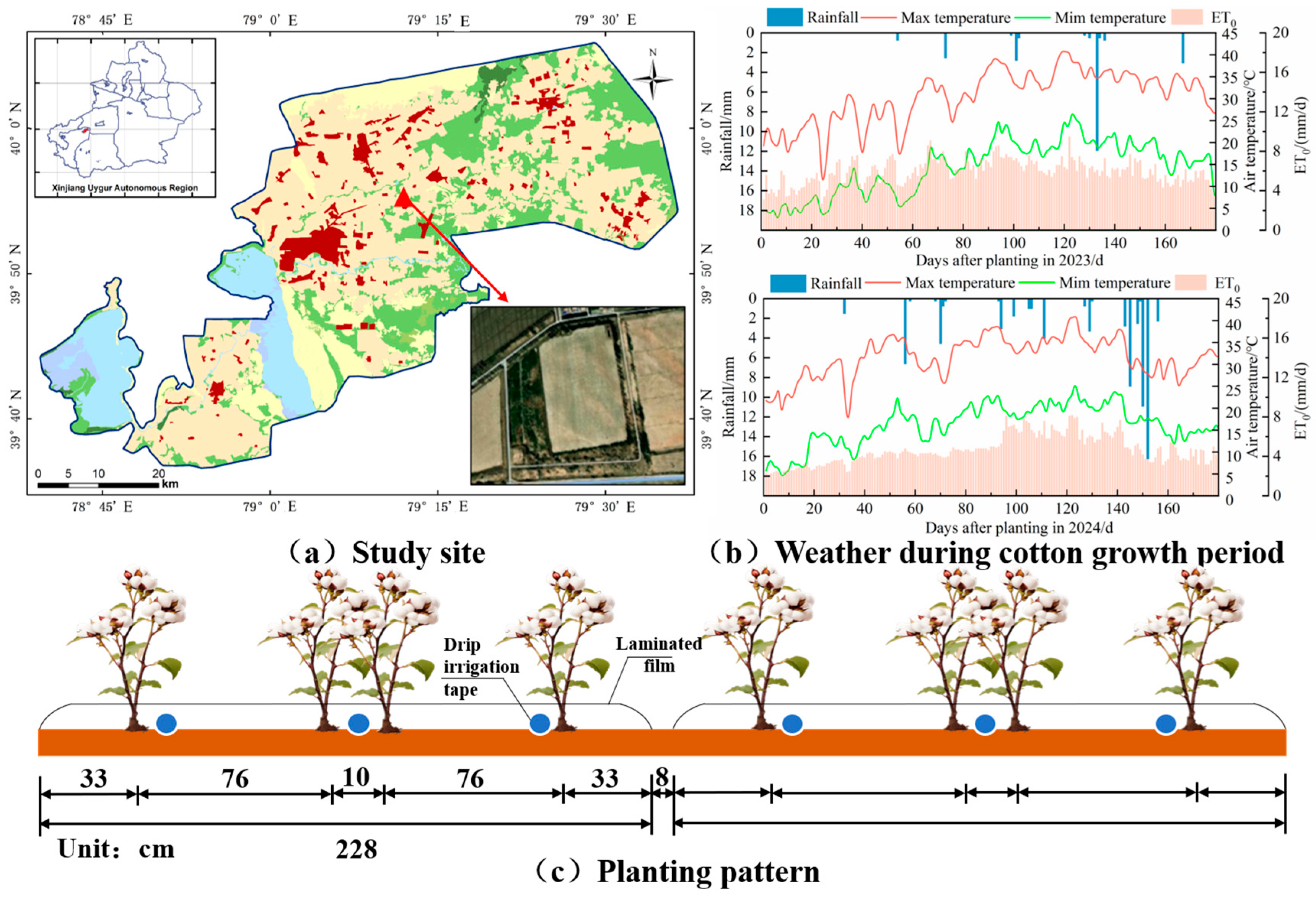
2.1. Overview of the Experimental Site

The experiment is located in the original seed production area of the 44th Regiment in Tumushuke City, Southern Xinjiang, which belongs to a temperate extreme arid desert climate, at an altitude of 1096 m. The temperatures for 2023 and 2024 were 13.13 °C and 16.74 °C, respectively, with precipitation during the growing season being 25.4 mm and 77.47 mm. The soil is sandy loam, with organic matter in the topsoil (0–20 cm) measuring 14.24 g/kg, available phosphorus at 10.96 mg/kg, available potassium at 43.84 mg/kg, and total nitrogen at 1.22 g/kg, with no influence from groundwater. The location of the experiment and the meteorological data for cotton during the growing seasons of 2023 and 2024 are shown in Figure 1a,b.

2.2. Experimental Design

The experiment was conducted from March to October in 2023 and 2024, using the cotton variety “Tahe No. 2”. The planting model implemented was one film, three pipes, and four rows (76 cm + 10 cm + 76 cm), with a drip irrigation method under the film. Integrated mechanical operations were used for sowing, mulching, and laying the drip irrigation tape, with a drip tape diameter of 16 mm, a spacing of 30 cm between emitters, a flow rate of 2.8 L/h, and a working pressure of 0.1 Mpa. Based on the local irrigation level of 600 mm, three irrigation levels are set: 360 mm (W1, 60%), 450 mm (W2, 75%), and 540 mm (W3, 90%). Each treatment was replicated three times, using a randomized block design, resulting in a total of 9 experimental plots, each with an area of 138.6 m² (60 m × 2.28 m), and a theoretical planting density of 11.68 × 104 plants/hm². The fertilization amount is based on the local level, with the total fertilization during the growth period being 750 kg/ha of urea, 161 kg/ha of diammonium phosphate, and 501 kg/ha of potassium fulvic acid. Specific fertilization measures are shown in

Table 1. Irrigation system in cotton growing period.

Cotton Growth Period	Duration of the Growth Period/ Month. Day–Month. Day		Irrigation Date/ Month. Day		Treatment/mm			Fertilizer Yield/(kg/hm2)
	2023	2024	2023	2024	W1	W2	W3	N	P	K
Emergence stage	03.24–04.20	03.27–04.24	03.24	03.27	11.5	11.5	11.5	0.0	0.0	0.0
			03.30	04.02	15.0	15.0	15.0	0.0	0.0	0.0
			04.17	04.20	30.0	30.0	30.0	0.0	0.0	0.0
Seedling stage	04.23–05.24	04.25–05.26	05.10	05.15	30.4	39.4	48.4	37.0	5.0	10.0
			06.02	06.04	30.4	39.4	48.4	40.0	5.0	23.0
Bud stage	05.25–06.23	05.27–06.21	06.12	06.13	30.4	39.4	48.4	40.0	5.0	23.0
			06.25	06.23	30.4	39.4	48.4	100.0	21.0	65.0
Florescence	06.24–07.14	06.22–07.12	07.02	06.30	30.4	39.4	48.4	100.0	21.0	65.0
			07.09	07.07	30.4	39.4	48.4	100.0	21.0	65.0
			07.16	07.14	30.4	39.4	48.4	100.0	21.0	65.0
Boll season	07.15–08.09	07.13–8.05	07.23	07.21	30.4	39.4	48.4	100.0	21.0	65.0
			07.30	07.28	30.4	39.4	48.4	100.0	21.0	65.0
Batting	08.10–10.07	08.06–09.26	08.13	08.11	30.4	39.4	48.4	33.0	20.0	55.0
Total	198 d	184 d	-	-	360.0	450.0	540.0	750.0	161.0	501.0

. The specific layout is shown in Figure 1c.

The dry sowing and wet emergence method for cotton involved an initial irrigation of 112.5 m³/hm², followed by 150 m³/hm² after 7 days, and 300 m³/hm² after 25 days. Before sowing, the base fertilizer applied included 375 kg/hm² of diammonium phosphate, 300 kg/hm² of urea, and 120 kg/hm² of potassium humate. In 2023, sowing, topping, and harvesting were conducted on 23 March, 16 July, and 7 October, respectively, while in 2024, these activities took place on 26 March, 2 July, and 26 September. After emergence, fertilization during the growing period was carried out using a “one water, one fertilizer” approach, with a total of 10 irrigations. The fertilizers used were urea (containing 46% N), diammonium phosphate (containing 64% P), and potassium humate (containing 55% K). The irrigation amount for each plot is controlled by a water meter and ball valve. Water-soluble fertilizers are weighed using balance and poured into a fertilization tank for irrigation. The physical properties of the soil in the experimental area are shown in

Table 2. Physical properties of soil in experimental area.

Soil Depth (cm)	Soil Bulk Density (g/cm3)	Field Capacity (g/g)	Saturated Water Content (g/g)	Clay Particles (%)	Powder Granules (%)	Sand Grain (%)	Wilting Coefficient (g/g)
0–20	1.45	0.21	0.28	17.80	30.85	51.35	0.07
20–40	1.46	0.22	0.31	20.68	27.23	52.09	0.08
40–60	1.48	0.24	0.32	20.53	27.35	52.12	0.10
60–80	1.51	0.24	0.29	19.52	25.93	54.55	0.09
80–100	1.51	0.22	0.28	19.62	24.21	56.17	0.08

, and the specific irrigation design is detailed in Table 1. Other field management practices were consistent with local standards.

2.3. Determination Items and Methods

2.3.1. Cotton Growth Index

For plant height, stem diameter, and leaf area index (LAI): After establishing the seedlings, 5 representative plants from each treatment were marked. Measurements were taken 45 days after cotton sowing using a tape measure and calipers, with measurements conducted every 7 days. For the selected plants, the length and width of the leaves were measured with a tape measure, and the leaf area was calculated using the empirical coefficient formula (length × width × 0.75). The formula for leaf area index is:

$$\mathrm{LAI}={\displaystyle \frac{{\mathrm{S}}_{\mathrm{LA}}{ \times S}_D}{\mathrm{10,000}}},$$

(1)

In the formula: S_LA represents the total leaf area of a single cotton plant, in m²/plant; S_D is the planting density, in plants/hm².

Above-ground dry biomass (B): The drying method was used, with samples taken once during each growth period. In each replicate treatment, 5 uniformly growing plants were selected, and the above-ground parts were cut and placed in an oven. They were subjected to a heat treatment at 105 °C for 0.5 h, followed by drying at 85 °C until a constant weight was achieved, after which they were cooled and weighed.

Canopy cover (CC): This can be calculated from the leaf area index, with the calculation formula being [17].

$$\mathrm{CC}=1.005{\left(1 - {\mathrm{e}}^{-0.6\mathrm{LAI}}\right)}^{1.2}$$

(2)

2.3.2. Soil Moisture Content

One day after each irrigation during the growth period, use a soil auger to collect soil samples between the membranes for each treatment, repeating the process three times. The drying method is used for measurement, with soil sampling depths of 10, 20, 30, 40, 50, 60, 70, 80, 90, and 100 cm. The formula for calculating moisture content is:

$$\mathrm{SWC}={\displaystyle \frac{{\mathrm{m}}_1-{\mathrm{m}}_2}{{\mathrm{m}}_2-{\mathrm{m}}_0}}\times 100\%,$$

(3)

In the formula: SWC is the gravimetric moisture content (%); m₀ is the mass of the aluminum box (g); m₁ is the total weight of the wet soil and the aluminum box (g); m₂ is the total weight of the dry soil and the aluminum box (g).

2.3.3. Yield and Composition

During the cotton flowering period, the yield of cotton is measured at the end of the season. For each treatment plot, a representative area of 4.56 m² (2.28 m × 2 m) with balanced growth is designated. Randomly selected cotton plants are sampled, and 100 cotton bolls are picked from the upper, middle, and lower layers in a ratio of 3:4:3. These bolls are weighed using an electronic balance (0.01 g), and the number of bolls per unit area, total plant count, hundred-boll weight, and single-boll weight are recorded. The actual harvested plant density is calculated, and the yield of standard seed cotton is converted for each plot based on the treatment area.

2.3.4. Irrigation Water Productivity

The calculation formula for irrigation water productivity (IWP, kg/m³), water productivity (WP, kg/m³) is:

$$\mathrm{IWP} ={\displaystyle \frac{\mathrm{Y}}{\mathrm{I}}}$$

(4)

$$\mathrm{W}\mathrm{P}=0.1{\displaystyle \frac{\mathrm{Y}}{{\mathrm{E}\mathrm{T}}_{\mathrm{a}}}}$$

(5)

$$ETa=P+I-D-\mathsf{\Delta }S-R$$

(6)

In the formula: Y represents the seed cotton yield, in kg/hm²; I represents the irrigation water amount during the whole growth period; ETa is the evapotranspiration amount; ΔS is the change in soil moisture before sowing and after harvest; P is the precipitation amount; D is the deep percolation; R is the runoff. All units are in mm (in this test area, the groundwater depth is relatively deep and the surface evaporation is strong, so both D and R are 0).

2.4. AquaCrop Model Introduction (Ver7.1)

2.4.1. Model Theory

The AquaCrop model is a model specifically designed to simulate crop growth, yield, and water productivity. The core principle of this model lies in accurately simulating the water balance and growth process of cotton, and then predicting the yield performance of cotton under different irrigation amounts and related management conditions, so as to explore the optimal irrigation amount for dry sowing and wet emergence cotton under the planting pattern. The model maintains soil water balance by quantifying water inputs (precipitation, irrigation) and outputs (evapotranspiration, deep percolation, surface runoff). The governing equation is expressed as:

$$\mathsf{\Delta }S=P+I-ET-D-R$$

(7)

In the formula: ΔS is the change amount of soil moisture, P is the precipitation amount, I is the irrigation amount, ET is the evapotranspiration amount, D is the deep seepage, and R is the runoff (the groundwater depth in the test area is relatively deep, and surface evaporation is intense, so both D and R are 0).

The model simulates crop growth by calculating the biomass accumulation (B, t/ha) and normalized water productivity (WP*, g/m²) of the crop. Firstly, the model uses the canopy cover (CC) curve to simulate the process of crop growth, development, and senescence, which is mainly determined by the initial CC (CC₀), canopy growth coefficient (CGC), maximum CC (CC_x), and canopy decline coefficient (CDC). The daily transpiration of the crop (Tc, mm/day) is separated from the reference evapotranspiration (ET₀, mm/day), and the calculation formula of the T_c value is:

$${\mathrm{T}}_{\mathrm{c}}={\mathrm{C}\mathrm{C}}^{\ast }\times {\mathrm{K}}_{\mathrm{c}\mathrm{T}\mathrm{r},\mathrm{x}}\times {\mathrm{E}\mathrm{T}}_0$$

(8)

In the formula, CC* is the actual canopy cover (%); K_cTr,x is the maximum transpiration coefficient of the crop under the condition of full irrigation and complete cover.

Then, AquaCrop uses the normalized water productivity to convert the crop transpiration into above-ground biomass as in Formula (9). The crop grain yield (Y, t/ha) is estimated from the final above-ground biomass and the harvest index (HI, %) as in Formula (10).

$$\mathrm{B}={\mathrm{W}\mathrm{P}}^{\ast }\times \sum {\mathrm{T}}_c$$

(9)

$$\mathrm{Y}={\mathrm{f}}_{\mathrm{H}\mathrm{I}}\times {\mathrm{H}\mathrm{I}}_0\times \mathrm{B}$$

(10)

In the formula, f_HI is the water stress coefficient of the harvest index, and HI₀ is the reference harvest index (%).

Soil water stress affects canopy cover development, root zone expansion, leads to stomatal closure, reduction of crop transpiration rate, pollination failure, changes the harvest index, and even triggers early canopy senescence. When the soil water stored in the root zone is lower than the threshold level, soil water stress will affect the above processes.

2.4.2. Meteorological Data

The data are provided by the Tumushuke Municipal Meteorological Bureau, mainly including the minimum (lmin) and maximum (lmax) temperatures, precipitation, solar radiation, and average wind speed, etc., and the parameters are adjusted according to the Penmen–Monteith formula recommended by the FAO to enable the model to calculate the reference crop evapotranspiration (ET₀) by itself. The meteorological data are shown in Figure 1.

2.4.3. Crop Data

The AquaCrop version 7.1 model itself provides a series of physiological parameters covering most typical crops, including cotton. Research on the calibration and application of the AquaCrop model by FAO over the years has shown that some parameters within the model do not change with geographical location, crop planting time, or field management practices, and these parameters are referred to as conservative parameters. Therefore, when conducting simulation calibration work, conservative parameters can be directly adopted from the calibration recommended values in the AquaCrop model manual. However, the remaining non-conservative parameters need to be localized and adjusted. The method is based on Xishan S and others [18], using the “trial and error method” combined with measured data for calibration. First, calibrate cotton canopy growth, then calibrate above-ground biomass, and finally, adjust the harvest index HI0 according to cotton yield. The final determined parameters are detailed in

Table 3. The main parameters of the Aquacrop model.

Argument	Item	Value	Unit
CC0	lnitial canopy cover	1	%
CCx	Maximum canopy cover	90	%
KcTR	Maximum canopy cover	1.1	-
Zx	Maximum root depth	0.6	m
Rexshp	Maximum root depth	0.5	cm/d
HI0	Reference yield index	38	%
Tbase	Base temperature	15	°C
Tupper	Ceiling temperature	35	°C
CGC	Canopy growth coefficient	10	%/d
CDC	Canopy attenuation coefficient	9	%/d
Kcbx	Crop coefficient when crop canopy is intact and not aged	1.03	-
Pexpupper	Upper limit of influence of water stress on canopy growth	0.3	-
Pexplower	Lower limit of influence of water stress on canopy growth	0.6	-
Eceupper	Upper threshold of salt effect on crop growth	4	dS/m
Ecelower	Lower threshold of salinity effect on crop growth	15	dS/m

.

2.4.4. Soil Data

The main parameters include soil texture, field capacity at each layer, saturated water content, permanent wilting point, and bulk density. The physicochemical properties were obtained through institutional testing and field measurements. These parameters are input into the model to generate a soil data file. The soil physical property parameters for the experimental site are presented in Table 2.

2.4.5. Field Data

Field data encompass irrigation schedules and field management practices, including crop irrigation regimes (number of irrigations, irrigation dates, and irrigation levels or amounts—detailed in Table 1), irrigation method (drip irrigation), soil fertility (moderate fertility), ground cover status (plastic film mulch), absence of surface runoff, and weed growth. These parameters were compiled to generate irrigation files representing three distinct irrigation regimes.

2.4.6. Model Evaluation

The AquaCrop model outputs were evaluated using field trial data from 2023 and 2024 through five statistical metrics. The field experiment data in 2023 are used to calibrate the key parameters of the AquaCrop model, while the data in 2024 are used to verify the simulation accuracy of the model: Root Mean Square Error (RMSE), Normalized Root Mean Square Error (NRMSE), Index of Agreement (d), Coefficient of Determination (R²), and Relative Error (RE), calculated via Equations (11)–(15). Lower values of NRMSE, RMSE, and RE indicate higher model accuracy. The Index of Agreement (d) approaching 1 demonstrates enhanced model precision with positive variable correlation, while approaching −1 reflects improved precision with negative correlation. Empirical studies generally consider R² > 0.8 as the threshold for reliable crop simulation modeling.

$$RMSE=\sqrt{{\displaystyle \frac{1}{n}}{\sum }_{i=1}^n{\left(P_i-O_i\right)}^2}$$

(11)

$$NRMSE={\displaystyle \frac{\sqrt{\frac{1}{n}{\sum }_{i=1}^n{(P_i-O_i)}^2}}{O_m}}\times 100$$

(12)

$$d=1-{\displaystyle \frac{{\sum }_{i=1}^n{(P_i-O_i)}^2}{{\sum }_{i=1}^n{\left(\right|P_i-O_m|+|O_i-O_m\left|\right)}^2}}$$

(13)

$$R^2=1-{\displaystyle \frac{{\int }_{i=1}^n\sum {(O_i-P_i)}^2}{{\int }_{i=1}^n\sum {(O_i-O_m)}^2}}$$

(14)

$$RE={\displaystyle \frac{O_i-P_i}{O_i}}\times 100$$

(15)

In the formula, n is number of observations; Pi is model-predicted value for the i-th observation; Oi is corresponding observed value; Om is mean of observed values.

2.4.7. Simulation Scenario Setting

Utilizing the calibrated parameters, multi-scenario simulations of the AquaCrop model were conducted. Meteorological data are output as a two-year average in a .CLI file, with field management set according to 2024. The total irrigation amount was set within the range of 360–660 mm with a gradient of 30 mm, establishing 11 irrigation scenarios, namely, I = 360, 390, 420, 450, 480, 510, 540, 600, 630, 660 mm, generating 11 irrigation management files .MAN. Other input parameters remain unchanged. These simulations aimed to determine the optimal irrigation regime through comprehensive analysis of water-saving effects and yield enhancement objectives.

2.5. Data Processing and Analysis

Data organization uses Excel 2023, plotting is conducted with Origin 2022 software, and significance analysis is conducted using SPSS 27 software.

3. Results

3.1. Effects of Different Irrigation Rates on Cotton Growth

Figure 2 shows the dynamic changes in cotton plant height, stem diameter, and LAI under different irrigation levels or amounts during the experimental period of two years, all of which had significant effects (p < 0.05). Under the same irrigation level or amount, the height and stem diameter of cotton rapidly increased as the growth cycle progressed, reaching a gradually stable state during the flowering period (90 days after sowing). During the stable growth stage of cotton, in 2023, the plant heights were as follows: 88.1 cm for treatment W1, 93.5 cm for treatment W2, and 102.3 cm for treatment W3; the stem diameters were, respectively, 11.3 mm for treatment W1, 12.5 mm for treatment W2, and 13.8 mm for treatment W3. The plant height of treatment W3 increased by 16.11% and 9% compared with treatments W1 and W2, respectively; the stem diameter increased by 22.12% and 10.4%. In 2024, the plant heights were, respectively, 97.4 cm for treatment W1, 103.8 cm for treatment W2, and 109.2 cm for treatment W3; the stem diameters were: 13.4 mm for treatment W1, 15.2 mm for treatment W2, and 17.5 mm for treatment W3. The plant height of treatment W3 increased by 12.11% and 5.2% compared with treatments W1 and W2, respectively; the stem diameter increased by 30.6% and 15.13%. The LAI changes exhibited a unimodal curve, reaching their peak at 115 days after sowing in both 2023 and 2024, with significant increases observed across treatments. The above analysis indicates that under the “one film, three pipes, four rows” planting model, high-level irrigation can significantly promote the growth and development of cotton.

3.2. Effects of Different Irrigation Amounts on Soil Gravimetric Moisture Content

As shown in Figure 3, the amount of irrigation affects the spatiotemporal distribution soil moisture in the 0–100 cm soil layer of cotton fields. The trend of soil moisture content changes is basically consistent throughout the growth period for all treatments. When irrigation amount increases, the soil’s moisture retention capacity is enhanced. As the growth period progresses, soil moisture content first increases and then decreases vertically, with minor differences in moisture content between treatments in the deeper layers (60–100 cm) and significant differences in the middle layers (30–60 cm). In 2023, the average soil moisture content in the 0–100 cm layer under treatment W3 was 7.11% and 3.52% higher than those under treatments W1 and W2, respectively. In 2024, the average soil moisture content under treatment W3 was 0.5% and 3.43% higher than those under treatments W1 and W2, respectively. From the mid-bud stage (80 days after sowing) onwards, as the root system grows and distributes, moisture is mainly stored in the middle soil layer, and at this time, the irrigation amount significantly affects cotton growth by increasing soil moisture content, with treatment W3 showing significantly higher soil moisture than treatments W1 and W2. After the late boll stage (124 days after sowing), the water demand of cotton decreases, and the overall soil moisture content in all treatments gradually declines. In summary, the soil moisture retention capacity under treatment W3 is superior to that under W1 and W2, aiding in water absorption and growth in the cotton root zone.

3.3. Effects of Different Irrigation Rates on Seed Cotton Yield, IWP, and WP

The effects of different irrigation amounts on the irrigation water productivity, yield and its composition of cotton are shown in

Table 4. WP, IWP, yield, and composition of cotton under different irrigation levels or amounts.

Year	Treatment	Number of Bolls per Plant/Piece	Single Boll Weight/g	Number of Harvested Plants × 104 Plant/ha	Seed Cotton Yield /(kg/ha)	WP (kg/m3)	IWP (kg/m3)
2023	W1	9.11 ± 0.1 c	5.62 ± 0.08 c	10.13 ± 0.11 c	5186.38 ± 102.98 c	1.40 ± 0.03 c	1.44 ± 0.04 c
	W2	9.35 ± 0.06 b	5.87 ± 0.09 b	10.38 ± 0.09 b	5697.01 ± 129.77 b	1.28 ± 0.01 b	1.27 ± 0.02 b
	W3	9.67 ± 0.12 a	6.32 ± 0.16 a	10.76 ± 0.09 a	6575.91 ± 134.45 a	1.23 ± 0.02 a	1.22 ± 0.01 a
2024	W1	9.82 ± 0.15 c	6.15 ± 0.12 c	9.04 ± 0.15 c	5459.53 ± 78.95 c	1.42 ± 0.03 c	1.52 ± 0.01 c
	W2	10.24 ± 0.9 b	6.38 ± 0.07 b	9.45 ± 0.11 b	6173.80 ± 156.11 b	1.36 ± 0.01 b	1.37 ± 0.01 b
	W3	10.62 ± 0.11 a	6.87 ± 0.14 a	9.94 ± 0.16 a	7252.16 ± 142.59 a	1.32 ± 0.03 a	1.34 ± 0.02 a

Note: 1. The data are presented as ‘mean ± standard error’. 2. Differences denoted by distinct lowercase letters within the same column are considered statistically significant at p < 0.05.

. The quantity of irrigation water exerts a highly significant promoting influence on the seed cotton yield (p < 0.01), and the seed cotton yield ascends with the augmentation of the irrigation amount. Among these, the seed cotton yield of treatment W3 is the highest. In 2023, it is 6575.91 kg/hm², and in 2024, it is 7252.16 kg/hm². Compared with the W1 and W2 treatments, it has increased by 26.79%, 15.43% and 32.84%, 17.47%, respectively, in the two years. Among them, the cotton boll weight per boll, the number of bolls per plant, and the number of harvested plants all show significance, and the W3 treatment performs the best in both years. IWP and WP first decrease with the increase in the irrigation level. In the two years, the W3 treatments are 1.22 kg/m³, 1.34 kg/m³ and 1.23 kg/m³, 1.32 kg/m³, respectively, which are averagely reduced by 13.46%, 2.96% and 9.48%, 3.36% compared with the W1 and W2 treatments. The above analysis shows that the cotton yield under the W3 treatment is the highest, while IWP and WP only decrease slightly.

3.4. Model Simulation and Evaluation

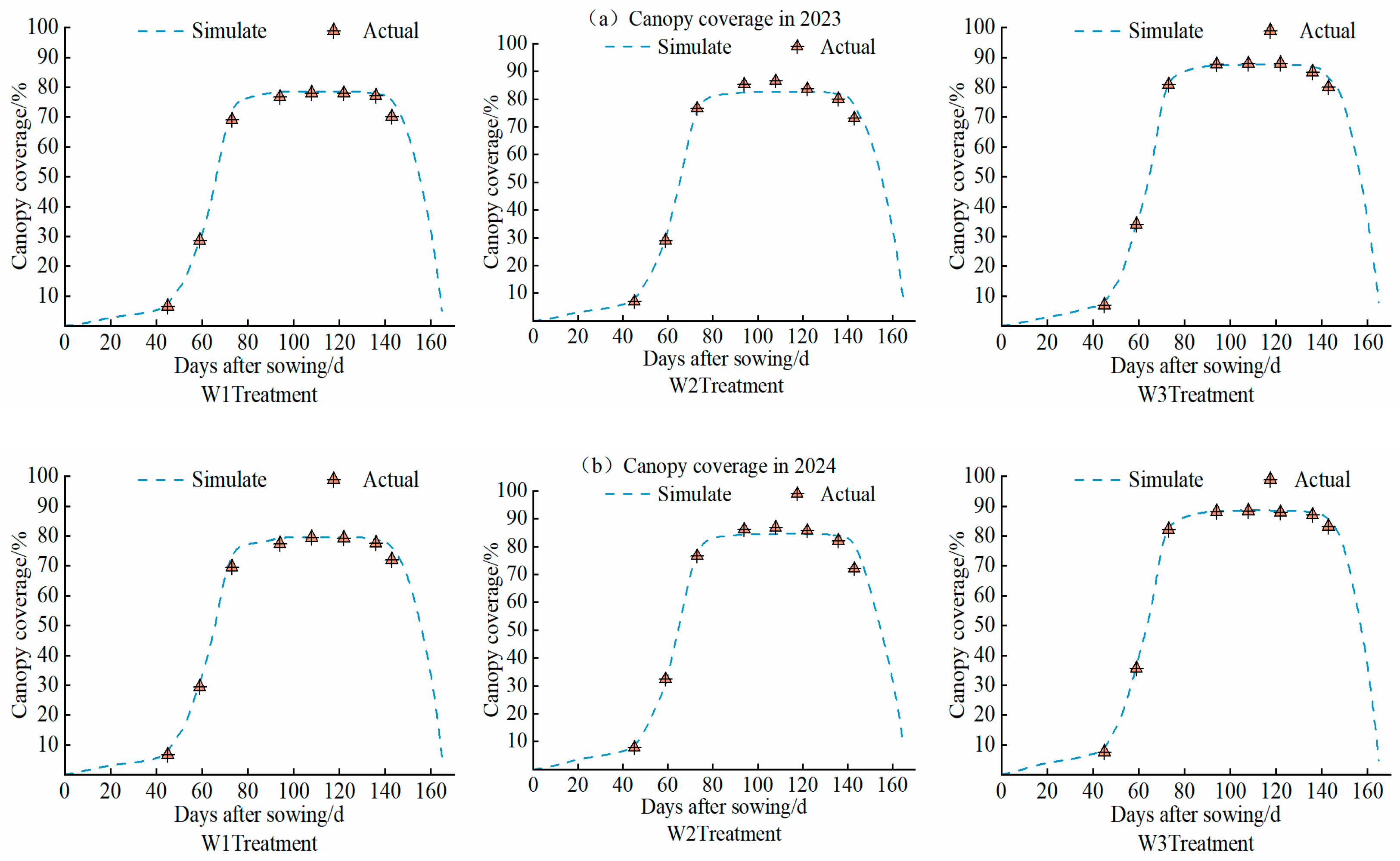
3.4.1. Canopy Cover

The accuracy of the model’s simulation results was evaluated using two years of data on cotton canopy cover, biomass, and yield, as shown in

Table 5. Accuracy evaluation of simulation results under different treatments of AquaCrop model.

Year	Index	Treatment	RMSE	NRMSE (%)	d	R2	RE (%)
2023	Canopy Cover (%)	W1	6.18	13.36	0.955	0.978	−1.27
		W2	4.14	15.60	0.967	0.982	4.33
		W3	3.42	8.27	0.988	0.976	1.52
	Biomass (t/hm2)	W1	0.39	12.24	0.915	0.934	−2.06
		W2	1.26	23.58	0.954	0.895	−3.65
		W3	1.03	15.98	0.928	0.903	−7.50
	WP (kg/m3)	-	0.23	5.85	0.924	0.915	0.37
	Yield (t/hm2)	-	0.71	10.24	0.933	0.912	5.11
2024	Canopy Cover (%)	W1	7.42	15.08	0.961	0.981	−1.35
		W2	5.57	11.45	0.972	0.967	2.42
		W3	4.11	9.22	0.984	0.984	1.22
	Biomass (t/hm2)	W1	2.54	10.46	0.921	0.964	−3.82
		W2	1.86	18.25	0.904	0.923	−4.70
		W3	1.14	13.41	0.942	0.931	−6.42
	WP (kg/m3)	-	0.12	5.33	0.933	0.881	1.02
	Yield (t/hm2)	-	0.79	8.35	0.941	0.923	4.27

. In the simulation of canopy cover, the W3 treatment had the best simulation accuracy over the two years, while the simulation accuracy for W1 and W2 was lower but still within an acceptable range. For each treatment, d ≥ 0.955, R² ≥ 0.967, and −1.35 ≤ RE ≤ 4.33, indicating excellent simulation accuracy of the module. The changes in canopy cover are shown in Figure 4. Before 45 days after sowing, the growth of canopy cover was slow. Subsequently, thanks to the dry sowing and wet emergence technique and sufficient water and fertilizer supply, canopy development accelerated, reaching a peak in canopy cover before 80 days and maintaining it for about 60 days. After 140 days, as the cotton aged, the canopy cover declined. The analysis shows that the simulation trend for each treatment was consistently in line with the measured trend throughout the growth period.

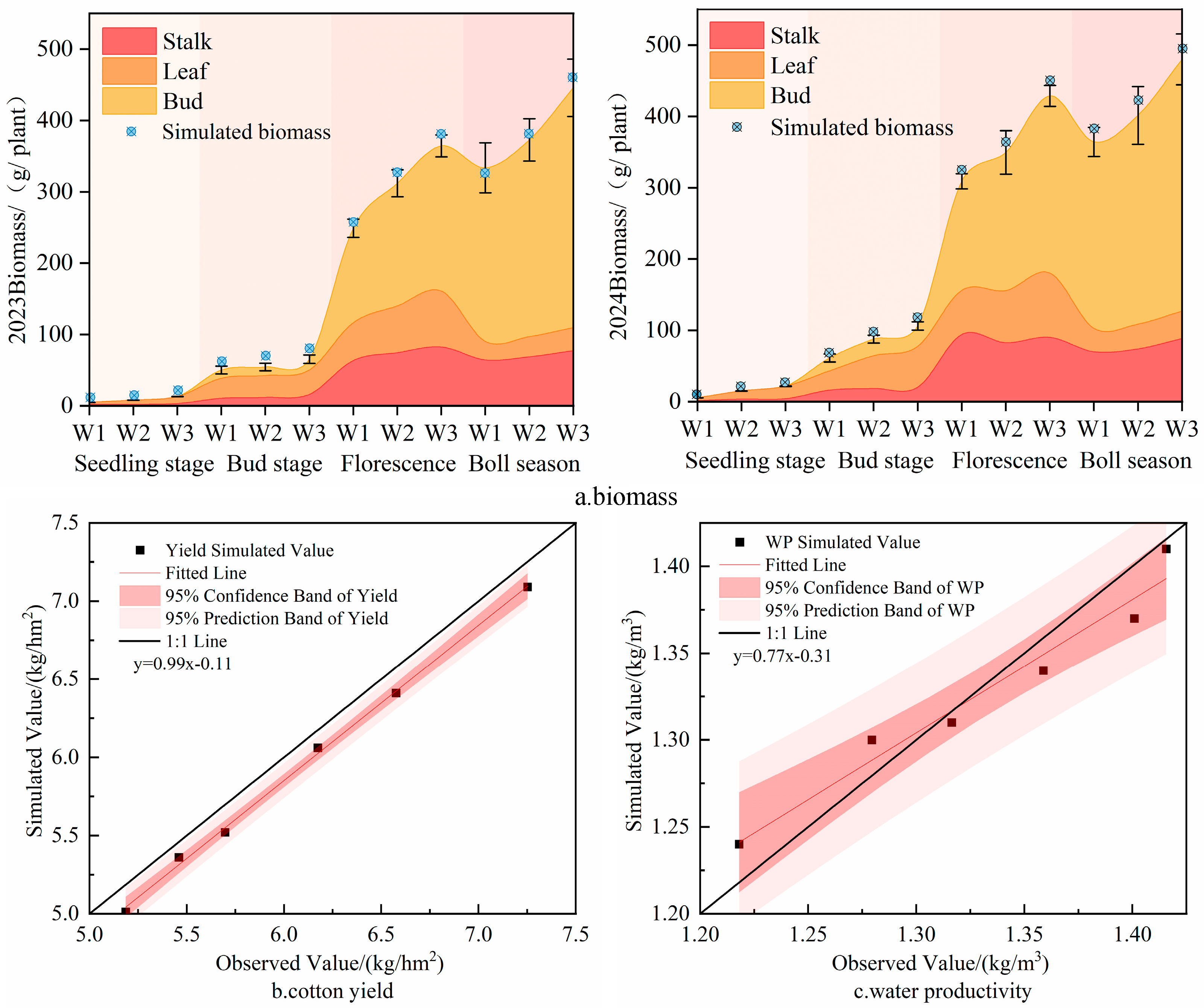
3.4.2. Biomass, Yield, and WP

The irrigation amount has a significant impact on the dry matter accumulation in different organs of cotton. In each growth stage of cotton over the two-year period, the order of above-ground dry matter mass and yield for each irrigation treatment is: W3 > W2 > W1, as depicted in Figure 5. Under varying irrigation treatments, the dry matter mass of cotton increases as the growth period progresses. It accumulates rapidly from the budding stage to the flowering stage and then stabilizes at the boll stage. Regarding the composition and distribution of dry matter, there are significant differences (p < 0.05) between the reproductive organs (buds) and the vegetative organs (stems and leaves) among the W1 and W2 treatments and the W3 treatment. With the increase in irrigation water amount, the dry matter accumulation in the reproductive organs gradually rises, and the leaves within the vegetative organs account for the major portion of the dry matter accumulation. During the flowering and boll stage, cotton attains the maximum dry matter mass under the W3 treatment. In 2023, it is 445.7 g/plant, which is 33.62% and 19.6% higher than the dry matter masses under the W1 and W2 treatments, respectively, at the same time. In 2024, it is 479.9 g/plant, which is 31.8% and 19.55% higher than the dry matter masses under the W1 and W2 treatments, respectively, at the same time. When comparing the dry matter mass simulated by the model with the measured value, there is no obvious disparity in each treatment. The accuracy assessment reveals values such as d ≥ 0.904, R² ≥ 0.895, −7.5% ≤ RE ≤ −2.06, 0.39 t/hm² ≤ RMSE ≤ 2.54 t/hm², and 10.46% ≤ NRMSE ≤ 23.58%.

The yield simulation values of each treatment are slightly lower than the measured values (R² = 0.912 in 2023, d = 0.933, and R² = 0.923 in 2024, d = 0.941), the error RE is less than 5.11%, and the gap is not obvious. The RE and NRMSE of WP are less than 1.02% and 5.85, which is better than the yield simulation accuracy. Therefore, the AquaCrop model has good applicability in the local area and can be used to simulate the dry matter mass, yield, and WP of cotton under different irrigation levels.

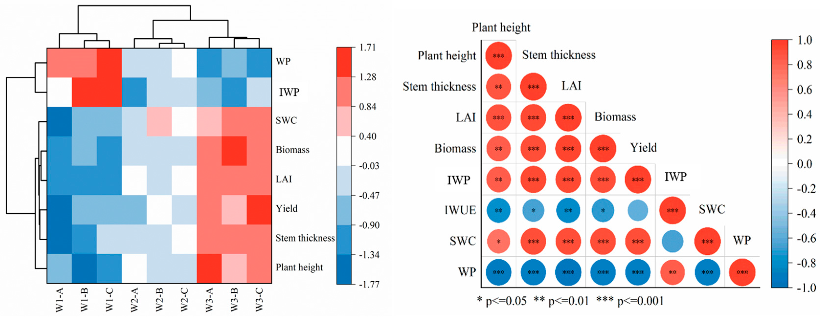
3.4.3. Heatmap Analysis

In order to compare the correlations between all indicators and treatments and determine the optimal combination, heat maps with hierarchical clustering and correlation heat maps were generated. As shown in Figure 6, it indicates the correlations among multiple growth and productivity indicators of cotton under different irrigation level treatments (W1, W2, W3) and their three repetitions (A, B, C). Under the low irrigation level, there is a significant negative correlation between cotton growth and yield, which indicates that under deficit irrigation conditions, these growth indicators may be affected by water limitations, while high-level irrigation significantly improves cotton growth and output. There is a significant positive correlation between WP and IWP, which shows that under sufficient water conditions, the improvement of water productivity contributes to the increase in water productivity. There is a significant positive correlation among plant height, stem diameter, LAI, biomass, and yield, and this relationship may reflect the synergistic effect of cotton growth, which promotes the efficiency of photosynthesis and the accumulation of biomass, and thereby increases the yield. There is a very significant positive correlation between SWC and WP, which indicates that the increase in soil water content may improve water productivity, which may be because sufficient water supply helps the growth and yield formation of plants. From the analysis, it can be obtained that high-level irrigation will strongly promote the growth and production of cotton in the arid area of Southern Xinjiang.

3.4.4. Multi-Scenario Simulation

Model scenario simulation can achieve a wider range of test results under limited test data and resources, saving human resources and time. After the calibration and evaluation of the AquaCrop model, 11 kinds of irrigation levels or amounts were simulated with a gradient of 30 mm to explore the cotton irrigation system that accurately realizes water-saving and yield-increasing. Figure 7 shows that with the increase in irrigation level or amount, the yield shows a trend of “increase—sharp increase—slow decrease”, and the IWP shows a trend of “decrease—slow decrease—sudden decrease”; when the irrigation amount is below 480 mm, the growth rate of seed cotton yield is relatively small, and between 480 mm and 570 mm, the seed cotton yield increases significantly, which may be because within this irrigation range, the water supply reaches the critical point that meets the cotton growth demand, thereby significantly promoting photosynthesis and growth rate; after exceeding 570 mm, the yield begins to decrease slightly and tends to be stable. Obviously, under the irrigation level or amount of 570 mm, the cotton yield reaches the highest value of 7.45 × 10³ kg/hm², and at this time, the IWP and WP reach the critical value of slow decrease, which are 1.307 kg/m³ and 1.294 kg/m³, respectively. Considering the irrigation cost and yield comprehensively, in the arid area of Southern Xinjiang, it is recommended to use the irrigation scheme with an irrigation level or amount of 570 mm to achieve sustainable agricultural production.

4. Discussion

4.1. The Impact of Different Irrigation Amounts on Cotton Growth and Soil

In arid regions, adjusting crop planting structures and optimizing water resource management are of great significance for the sustainable development of oases [19,20]. Different irrigation amounts significantly affect the growth of dry-sown and wet-harvested cotton. The low water supply in the W1 treatment inhibited the accumulation during the early nutritional stage of cotton, leading to an earlier reproductive growth period, which resulted in insufficient development of the cotton and reduced dry matter quality accumulation [21]. As the irrigation amount increased, the height, stem diameter, and leaf area of the cotton showed significant improvement. The growth advantage of cotton plants under the W3 treatment was most pronounced during the growth period, possibly because the higher water supply improved the moisture status of the plants, resulting in a larger leaf area index (LAI), thereby promoting photosynthesis and the synthesis and accumulation of dry matter [22]. The flowering and boll period is an important growth stage where nutritional and reproductive growth advance together, and sufficient water supply is necessary to ensure dry matter accumulation and yield formation [23]. Research on the dynamic distribution of soil moisture in field drip irrigation is of great significance for determining irrigation amounts and saving water while increasing yield [24]. The distribution of soil moisture after irrigation in the field showed that the moisture content in the 0–40 cm soil layer under the W3 treatment was closer to the field capacity, providing better soil moisture conditions for the growth during the cotton bud and flowering periods. However, Bi Wenping et al. [25] argued that 125% of the irrigation water requirement could not improve the soil moisture content in the root zone, and excessive irrigation could lead to strong transpiration, reducing soil moisture content. This discrepancy may be due to different soil structures, planting models, and meteorological influences in the experimental area compared to the results of this experiment. Throughout the entire growth period of cotton, high irrigation promoted the vertical movement of soil moisture, especially during the flowering and boll period, where the moisture retention effect in the 30–60 cm soil layer was significant. Reasonable irrigation is beneficial for the growth of cotton root systems to improve yield.

Improving water productivity and crop yield is key to the effective utilization of agricultural resources. Liu et al. [26] found that limited irrigation can enhance cotton moisture, but if the irrigation depth is too low, although a higher water productivity can be achieved, it will significantly reduce crop yield. Irrigation can improve the effectiveness of fertilization and the ability to absorb nutrients. Under all irrigation levels, the W3 treatment had the best single boll weight, number of bolls per plant, and cotton plant density, resulting in the highest seed cotton yield, which is beneficial for the stable development of local cotton production. This is consistent with the findings of Zhang Jun et al. [27] who indicated that a 60 mm irrigation level or amount is the optimal drip irrigation strategy, and reasonably increasing the irrigation amount can effectively improve yield while maintaining a negligible decline in irrigation water productivity (IWP). This may be because, under high-level irrigation, cotton grows vigorously, rapidly accumulating dry matter, resulting in a high final accumulation, with more branches and leaves extending, leading to a larger canopy cover area, which increases the shading area on the soil and suppresses the intense evaporation effect in Southern Xinjiang. This aligns with the research results of Li et al. [28]. From the analysis, it can be concluded that under the one film, three pipes, and four rows narrow-wide row model, a 540 mm irrigation level or amount can achieve high yield. Future research could include treatments with one film, six rows, and one film, three rows planting models to further explore the response of cotton growth to irrigation systems under different planting models.

4.2. Optimization of Irrigation Regimes Based on the AquaCrop Model

The article conducts research on the dry sowing with wet irrigation cotton experiment in 2023, calibrates the crop and irrigation parameters of the AquaCrop model, and introduces five different evaluation indicators. It analyzes the simulation results and the experimental data in 2024 to test the simulation accuracy of the model. A comprehensive comparison of the simulation effects of crop growth under different irrigation levels or amounts reveals that high-level irrigation can narrow the gap between simulated and measured values, which is consistent with the conclusions of Song Xishan et al. [18]. For canopy cover and biomass simulation, the former has better simulation accuracy than the latter, with canopy cover simulation values and measured values for each treatment having R² ≥ 0.967 and d ≥ 0.955, and the trend consistent with measured values, aligning with Amir et al. [29]. Simulated dry matter quality is satisfactory before the flowering stage but higher than measured values afterward, possibly due to strong evaporation, extreme temperature changes, and low precipitation in Tumushuke City during summer. The AquaCrop model simulates cotton dry matter quality in Tumushuke City higher during the flowering stage, but the yield simulation effect is better, with d being 0.933 and NRMSE being 10.24% in 2023, and d being 0.941 and NRMSE being 8.35% in 2024. Wang Xingpeng et al. [30] optimized the cotton irrigation system using AquaCrop in Aral City, Southern Xinjiang, with yield d and NRMSE being 0.84 and 14.02%, respectively, indicating minor deviations from actual observed values but satisfactory simulation accuracy. WP simulation results match actual test results. Analysis shows that the AquaCrop model can accurately simulate cotton canopy cover, biomass, WP, seed cotton yield, and their variation processes in Tumushuke City, Southern Xinjiang. Considering the large diurnal temperature differences and climate change instability in Southern Xinjiang, it is anticipated that the model can improve biomass and yield simulation results through multiple calibrations and temperature compensation [31].

Preliminary field trial results on irrigation system optimization indicate significant impacts of different irrigation levels or amounts on cotton growth and irrigation water productivity. After comprehensively considering IWP and yield output, the optimal irrigation treatment is W3. Subsequently, 11 different irrigation scenarios are simulated and analyzed based on the AquaCrop model, enhancing the study’s broad applicability and repeatability [32]. Model evaluation results show that when the irrigation level or amount reaches 480 mm, cotton yield begins to increase significantly, peaking at 570 mm; at this irrigation level, water productivity reaches a critical point of decline, maximizing seed cotton yield. However, further increasing irrigation amounts results in yield not increasing but instead declining and stabilizing. This phenomenon indicates that excessive irrigation may increase water stress, leading to a decrease in seed cotton yield. This is consistent with the simulation results of Juan Y et al. [33]. The study found that when applying drip irrigation technology in arid regions of the northwest, the yield increases with the increase in the total irrigation amount. However, when it exceeds a certain specific amount, the yield begins to decline, indicating that there is a threshold for the irrigation amount when achieving the optimal yield. Considering irrigation costs and yield benefits, the study recommends an irrigation scheme of 570 mm in arid regions of Southern Xinjiang. Appropriately increasing irrigation levels or amounts can not only maximize cotton yield but also have significant advantages in water conservation; this is consistent with the simulation results of Tingting J et al. [34], where high water irrigation in arid areas more significantly improves crop yield. Reasonable irrigation management strategies contribute to the sustainability of agricultural production, reduce resource waste and lower production costs, conform to the principles of a circular economy, and promote the coordinated development of agricultural production and the ecological environment. Through AquaCrop model simulation and field trial evaluation, aiming at water conservation and yield increase, it is recommended that for the dry sowing and wet emergence cotton cultivation in Southern Xinjiang under the planting mode of one film with three tubes and four rows, the irrigation system of 570 mm should be adopted. The research results will help scientifically manage cotton planting in arid regions of Southern Xinjiang, promoting sustainable agricultural development.

5. Conclusions

This study in the arid regions of Southern Xinjiang investigated the effects of different irrigation levels or amounts on the growth of cotton using a one-film, three-pipe, four-row planting method and soil moisture content. Based on AquaCrop simulations and evaluations, the results indicate the following:

(1)

High-level irrigation is beneficial for promoting the growth and development of cotton in arid areas, accumulating dry matter, and thereby increasing yield. The IWP and WP treatments showed W1 > W2 > W3, while yield exhibited W3 > W2 > W1. With the goal of achieving high yield while ensuring water conservation, the W3 treatment was optimal, averaging 1.28 kg/m³, 1.27 kg/m³, and 6914.04 kg/ha over two years.

(2)

Under drip irrigation with film cover, high-level irrigation effectively preserves moisture in the 30–60 cm soil layer of cotton fields. Compared to W1 and W2 treatments, the W3 treatment increased SWC by 8.26% and 3.23%, which is conducive to root absorption and growth development of cotton.

(3)

The AquaCrop model can accurately simulate the canopy cover, biomass, WP, yield, and their variation processes of cotton in saline-alkali land in Tumshuk City, Southern Xinjiang. Based on 11 scenario simulations using the AquaCrop model, as irrigation levels or amounts increase, WP and IWP show an inverse relationship, while yield initially increases and then slowly declines. Combining field data and simulation results, with the goals of water conservation and yield increase, it is recommended that in Southern Xinjiang, for dry sowing with wet irrigation cotton under the planting pattern of one film, three tubes, and four rows, a 570 mm irrigation regime should be used.

References

1. Ding, Y.; Ma, J.; Zhang, J.; Bai, Y.; Cui, B.; Hao, X.; Fu, G.; Zheng, M.; Ding, B. Response of photosynthesis, population physiological indexes, and yield of cotton in dry areas to the new technology of “dry sowing and wet emergence”. Front. Plant Sci. 2024, 15, 1487832. [Google Scholar] [CrossRef]
2. Cui, Y.S.; Wang, F.; Sun, J.S.; Han, Q.S.; Wang, J.L.; Li, N. Effects of irrigation regimes on the variation of soil water and salt and yield of mechanically harvested cotton in Southern Xinjiang, China. Chin. J. Appl. Ecol. 2018, 29, 3634–3642. [Google Scholar] [CrossRef]
3. Wu, F.; Tang, Q.; Zhang, L.; Cui, J.; Tian, L.; Guo, R.; Wang, L.; Chen, B.; Zhang, N.; Ali, S.; et al. Reducing Irrigation and Increasing Plant Density Enhance Both Light Interception and Light Use Efficiency in Cotton under Film Drip Irrigation. Agronomy 2023, 13, 2248. [Google Scholar] [CrossRef]
4. Cui, Y.; Gao, Z.; Yang, B. Quality analysis of different mechanical harvesting cotton planting patterns. J. Chin. Agric. Mech. 2016, 37, 235–240. [Google Scholar] [CrossRef]
5. Hu, L.; Pan, X.; Wang, X.; Hu, Q.; Wang, X.; Zhang, H.; Xue, Q.; Song, M. Cotton photosynthetic productivity enhancement through uniform row-spacing with optimal plant density in Xinjiang, China. Crop Sci. 2021, 61, 2745–2758. [Google Scholar] [CrossRef]
6. Wang, L.; Liu, G.; Ning, H.; Han, Q.; Xv, X.; Wang, X.; Li, X. Effects of Different Planting Patterns and Irrigation Quota on Cotton Growth and Yield. J. Irrig. Drain. 2023, 42, 16–23. [Google Scholar] [CrossRef]
7. Li, J.; Wu, P.; Xiao, S.; Cui, J.; Zhang, J. Effects of cotton planting modes with machine picking on defoliation and fiber quality of different plant types. J. Irrig. Drain. 2019, 37, 82–88. [Google Scholar]
8. Shukr, H.H.; Pembleton, K.G.; Zull, A.F.; Cockfield, G.J. Impacts of Effects of Deficit Irrigation Strategy on Water productivity and Yield in Cotton under Different Irrigation Systems. Agronomy 2021, 11, 231. [Google Scholar] [CrossRef]
9. Maucieri, C.; Borin, M.; Morbidini, F.; Pogačar, T.; Flajšman, M.; Ghinassi, G.; Verdi, L.; Dalla Marta, A.; Ferrise, R. Projecting the impacts of climate change on soybean production and water requirements using AquaCrop model. Eur. J. Agron. 2025, 165, 127538. [Google Scholar] [CrossRef]
10. Silvia, L.; Wilfredo, B.; Leonardo, V.; Carlo, N.; Anna, D.M.; Carmelo, M. Modelling the response of tomato on deficit irrigation under greenhouse conditions. Sci. Hortic. 2024, 326, 112770. [Google Scholar]
11. Zeeshan, S.S.; Xurong, M.; Buchun, L.; Yuan, L. Assessment of the AquaCrop Model under different irrigation scenarios in the North China Plain. Agric. Water Manag. 2021, 257, 107120. [Google Scholar]
12. Linker, R.; Ioslovich, I. Assimilation of canopy cover and biomass measurements in the crop model AquaCrop. Biosyst. Eng. 2017, 162, 57–66. [Google Scholar] [CrossRef]
13. Jorge, A.-B.; Coulibaly, S.; Baki, G.; Luís, C.J.; Abdalla, D.; Baptiste, M.J.; Dalla, M.A. Using AquaCrop as a decision-support tool for improved irrigation management in the Sahel region. Agric. Water Manag. 2023, 287, 108430. [Google Scholar]
14. Ahmadi, S.H.; Mosallaeepour, E.; Kamgar-Haghighi, A.A.; Sepaskhah, A.R. Modeling Maize Yield and Soil Water Content with AquaCrop Under Full and Deficit Irrigation Managements. Water Resour. Manag. 2015, 29, 2837–2853. [Google Scholar] [CrossRef]
15. Zhang, J.; Li, K.; Gao, Y.; Feng, D.; Zheng, C.; Cao, C.; Sun, J.; Dang, H.; Hamani, A.K. Evaluation of saline water irrigation on cotton growth and yield using the AquaCrop crop simulation model. Agric. Water Manag. 2022, 261, 107355. [Google Scholar] [CrossRef]
16. Wang, H.; Li, G.; Xu, X.; Huang, W.; Zhao, Z.; Gao, Y.; Wang, X. Assessing the Sustainability of Cotton Production under Climate Change Based on the AquaCrop Model. Chin. J. Agrometeorol. 2023, 44, 588–598. [Google Scholar]
17. Hsiao, T.C.; Heng, L.; Steduto, P.; Rojas-Lara, B.; Raes, D.; Fereres, E. AquaCrop—The FAO Crop Model to Simulate Yield Response to Water: III. Parameterization and Testing for Maize. Agron. J. 2009, 101, 448–459. [Google Scholar] [CrossRef]
18. Song, X.; Cao, H.; He, Z.; Ding, B.; Yao, N. Applicability of the Aquacrop model in optimization of irrigation and salt leaching schedule during the reproductive period of cotton in Northern Xinjiang of China. Trans. Chin. Soc. Agric. Eng. 2023, 39, 111–122. [Google Scholar]
19. Liu, Y.; Gui, D.; Chen, X.; Liu, Q.; Zeng, F. Sap flow characteristics and water demand prediction of cash crop in hyper-arid areas. Agric. Water Manag. 2024, 295, 108767. [Google Scholar] [CrossRef]
20. Yao, H.; Zhang, Y.; Yi, X.; Zuo, W.; Lei, Z.; Sui, L.; Zhang, W. Characters in light-response curves of canopy photosynthetic use efficiency of light and N in responses to plant density in field-grown cotton. Field Crops Res. 2017, 203, 192–200. [Google Scholar] [CrossRef]
21. Wang, N.; Feng, K.; Nan, H.; Cong, A.; Zhang, T. Effects of Combined Application of Organic Manure and Chemical Fertilizer Ratio on Water and Nitrogen Use Efficiency of Cotton Under Water Deficit. Sci. Agric. Sin. 2023, 56, 1531–1546. [Google Scholar]
22. Hui, Z.; Kai, Z.; Bing, C.; Chuan, Y.; Ping, L. Effects of different irrigation rates on cotton growth and yield formation in Xinjiang. Arid Zone Res. 2022, 39, 1976–1985. [Google Scholar] [CrossRef]
23. Zheng, J.; Li, Z.; Zhang, Y.; Yang, Y.; Chen, G.; Luo, X. Effects of applying water and nitrogen on soil inorganic nitrogen distribution and yield in cotton at stage of flowering and bolling. J. Huazhong Agric. Univ. 2023, 42, 105–112. [Google Scholar] [CrossRef]
24. Du, K.; Qiao, Y.; Zhang, Q.; Li, F.; Li, Q.; Liu, S.; Tian, C. Modeling Soil Water Content and Crop-Growth Metrics in a Wheat Field in the North China Plain Using RZWQM2. Agronomy 2021, 11, 1245. [Google Scholar] [CrossRef]
25. Bi, W.; Lin, D.; Mao, X. Two-dimensional transport of soil water, heat and salt with mulched drip irrigation under brackish water in cotton fields and appropriate irrigation schedule in southern Xinjiang of China. Trans. Chin. Soc. Agric. Eng. 2024, 40, 155–168. [Google Scholar]
26. Liu, X.; Liu, J.; Huang, C.; Liu, H.; Meng, Y.; Chen, H.; Ma, S.; Liu, Z. The impacts of irrigation methods and regimes on the water and nitrogen utilization efficiency in subsoiling wheat fields. Agric. Water Manag. 2024, 295, 108765. [Google Scholar] [CrossRef]
27. Zhang, J.; Wang, X.; Cui, X.; Li, A.; Zhao, L.; Hu, T. Effects of irrigation amount and nitrogen synergists on yield and utilization of water and fertilizer of summer maize. Agric. Res. Arid Areas 2024, 42, 123–132+168. [Google Scholar] [CrossRef]
28. Li, N.; Shi, X.; Zhang, H.; Shi, F.; Zhang, H.; Liang, Q.; Hao, X.; Luo, H.; Wang, J. Optimizing irrigation strategies to improve the soil microenvironment and enhance cotton water productivity under deep drip irrigation. Agric. Water Manag. 2024, 305, 109095. [Google Scholar] [CrossRef]
29. Amir, A.; Naghi, Z.A.; Mohammadreza, N.S.; Parviz, R.M.; Mahdi, G.S. Simulation of saffron growth using AquaCrop model with high-resolution measured data. Sci. Hortic. 2024, 324, 112569. [Google Scholar]
30. Wang, X.; Jiang, F.; Wang, H.; Cao, H.; Yang, Y.; Gao, Y. Irrigation Scheduling Optimization of Drip-irrigated without Plastic Film Cotton in South Xinjiang Based on Aqua Crop Model. Trans. Chin. Soc. Agric. Mach. 2021, 52, 293–301+335. [Google Scholar]
31. Chao, Z.; Jiying, K.; Min, T.; Wen, L.; Dianyuan, D.; Hao, F. Improving maize growth and development simulation by integrating temperature compensatory effect under plastic film mulching into the AquaCrop model. Crop J. 2023, 11, 1559–1568. [Google Scholar]
32. Tang, P.; Li, N.; Li, M.; Zhang, F.; Fu, Q.; Xu, Y.; Liu, D. Rice irrigation water efficiency improvement: An AquaCrop-based optimization modeling approach. Eur. J. Agron. 2023, 148, 126867. [Google Scholar] [CrossRef]
33. Yin, J.; Yang, Y.; Eeswaran, R.; Yang, Z.; Ma, Z.; Sun, F. Irrigation scheduling for potatoes (Solanum tuberosum L.) under drip irrigation in an arid region using AquaCrop model. Front. Plant Sci. 2023, 14, 1242074. [Google Scholar] [CrossRef] [PubMed]
34. Jiang, T.; Sun, S.; Li, Z.; Li, Q.; Lu, Y.; Li, C.; Wang, Y.; Wu, P. Vulnerability of crop water footprint in rain-fed and irrigation agricultural production system under future climate scenarios. Agric. For. Meteorol. 2022, 326, 109164. [Google Scholar] [CrossRef]
Figure 1. Test site location, cotton growing season weather, and planting pattern diagram.
Agronomy 15 01101 g001
Figure 2. Error band line chart of plant height, stem diameter, and leaf area index over time under different irrigation levels or amounts.
Agronomy 15 01101 g002
Figure 3. Graph of 0–100 cm soil water content (SWC) over time under different irrigation amounts.
Agronomy 15 01101 g003
Figure 4. Simulation and measurement of cotton canopy cover under different irrigation levels or amounts.
Agronomy 15 01101 g004
Figure 5. Simulation results of cotton biomass, yield, and WP under different irrigation levels for 2023–2024.
Agronomy 15 01101 g005
Figure 6. The variables of the clustering heat map and the correlation heat map include water productivity (WP), irrigation water productivity (IWP), soil water content (SWC), biomass (Biomass), leaf area index (LAI), yield (Yield), stem thickness (Stem thickness), and plant height (Plant height). The color gradient indicates the strength and direction of the correlation; red indicates a positive correlation and blue indicates a negative correlation. The depth of the color reflects the strength of the correlate.
Agronomy 15 01101 g006
Figure 7. Scenario simulation results and fitting of cotton yield, IWP, and WP under different irrigation levels or amounts.
Agronomy 15 01101 g007