Federated LeViT-ResUNet for Scalable and Privacy-Preserving Agricultural Monitoring Using Drone and Internet of Things Data

Abstract

Precision agriculture is necessary for dealing with problems like pest outbreaks, a lack of water, and declining crop health. Manual inspections and broad-spectrum pesticide application are inefficient, time-consuming, and dangerous. New drone photography and IoT sensors offer quick, high-resolution, multimodal agricultural data collecting. Regional diversity, data heterogeneity, and privacy problems make it hard to conclude these data. This study proposes a lightweight, hybrid deep learning architecture called federated LeViT-ResUNet that combines the spatial efficiency of LeViT transformers with ResUNet’s exact pixel-level segmentation to address these issues. The system uses multispectral drone footage and IoT sensor data to identify real-time insect hotspots, crop health, and yield prediction. The dynamic relevance and sparsity-based feature selector (DRS-FS) improves feature ranking and reduces redundancy. Spectral normalization, spatial–temporal alignment, and dimensionality reduction provide reliable input representation. Unlike centralized models, our platform trains over-dispersed client datasets using federated learning to preserve privacy and capture regional trends. A huge, open-access agricultural dataset from varied environmental circumstances was used for simulation experiments. The suggested approach improves on conventional models like ResNet, DenseNet, and the vision transformer with a 98.9% classification accuracy and 99.3% AUC. The LeViT-ResUNet system is scalable and sustainable for privacy-preserving precision agriculture because of its high generalization, low latency, and communication efficiency. This study lays the groundwork for real-time, intelligent agricultural monitoring systems in diverse, resource-constrained farming situations.

1. Introduction

Agriculture has long served as the foundation of societal development and human progress. Over time, it has evolved dramatically, from using rudimentary tools by early farmers to adopting sophisticated digital technologies in today’s smart farming. One of the most impactful developments in recent years is precision agriculture, which leverages data to understand and respond to variability in soil and crop conditions [1]. This approach helps farmers to use resources more efficiently, reduce environmental impact, and boost productivity.

Traditional agricultural methods like manual pest inspection and widespread pesticide spraying are becoming increasingly inadequate [2]. These methods are time-consuming and labor-intensive and pose risks to ecosystems and human health. As agriculture faces rising challenges such as pest outbreaks, climate variability, soil degradation, and water scarcity [3], there is a growing need for intelligent, automated systems to support sustainable and resilient farming. This is where unmanned aerial vehicles (UAVs) are making a real difference. Using high-resolution cameras—ranging from RGB to multispectral and thermal—UAVs can rapidly scan large fields and capture detailed information that ground-level surveys often miss [4,5].

Alongside UAVs, remote sensing techniques have introduced powerful tools like the NDVI and SAVI, which provide early signals of crop stress, disease, and nutrient deficiency [6]. When these time-series data are analyzed over time, they can help to predict crop growth stages and potential yield. Yet, even with these advancements, many challenges persist. Monitoring the interaction of various factors—such as soil moisture, temperature, pest density, and plant canopy—is complex [7]. For example, while increased soil moisture may benefit plant growth, it might also create favorable conditions for pests and diseases. Addressing such interdependencies requires more than just data—it demands intelligent models that can understand and adapt to these relationships.

Detecting pests early remains particularly difficult. Pests often appear in small, localized patches and are easy to miss. Their behaviors vary by species and region, making early classification even more challenging. However, recent progress in imaging and machine learning has opened up new possibilities for automating pest detection and classification, reducing the need for manual inspection [8]. At the same time, accurately forecasting yields has become a key goal in precision agriculture, helping farmers to plan resource use, storage, and market logistics. When trained on vegetation indices, soil parameters, and climate data, machine learning models can produce yield predictions that are both timely and reliable.

An emerging solution in this evolving landscape is federated learning (FL), which enables collaborative model training across multiple decentralized sources while keeping the raw data local [9]. This approach eliminates the need to transfer sensitive agricultural data to a central server, thereby enhancing both privacy and scalability. This decentralized training approach protects sensitive information and adapts well to the natural variability found across farms, crops, and climates. When combined with UAV-based systems, FL enables the creation of intelligent models that are location-aware and privacy-preserving.

Recent studies have shown that UAVs can track temperature changes, monitor soil conditions, and identify pest activity in real time [10]. By integrating machine learning, these systems enable precision-driven actions—such as applying pesticides only where needed or adjusting irrigation in specific zones—significantly reducing their environmental footprint. This convergence of drone technology, sensor networks, artificial intelligence, and federated learning marks a transformative shift in agriculture, paving the way for smarter, more sustainable practices that enhance productivity while preserving natural resources.

Motivation and Contributions: While recent research has explored deep learning for agricultural monitoring, many existing approaches fall short in terms of scalability, privacy, and the ability to handle heterogeneous sensor data in distributed environments. To address these gaps, we introduce a novel framework combining efficient deep learning, federated training, and adaptive feature selection tailored for UAV-driven agricultural analytics.

In this work, we propose Federated LeViT-ResUNet, a hybrid model that combines LeViT’s lightweight transformer-based feature extractor with the pixel-level segmentation power of ResUNet. To enhance interpretability and efficiency, we introduce a dynamic relevance and sparsity-based feature selector (DRS-FS) that focuses the model’s attention on the most meaningful inputs. Our federated framework enables model training directly on distributed edge devices—such as drones or on-site farm systems—while ensuring that sensitive data remain local and private. We train and evaluate the system using a large, open-access agricultural dataset with annotated segmentation masks and bounding boxes. Our experimental analysis shows that the proposed model achieves high accuracy, robust performance under varying environmental conditions, and better generalization than several state-of-the-art hybrid architectures.

The key contributions of this study are as follows:

• LeViT-ResUNet Hybrid Architecture: A lightweight, accurate model that blends LeViT’s efficient transformer backbone with ResUNet’s detailed segmentation for UAV-based agricultural monitoring.
• Federated Learning Integration: A decentralized training mechanism that supports privacy, scalability, and cross-regional adaptability in data-rich agricultural environments.
• Dynamic Feature Selection: A novel DRS-FS module that improves model focus and reduces overhead by selecting the most contextually relevant features.
• Comprehensive Preprocessing Framework: A robust pipeline that includes spectral normalization, noise removal, spatial–temporal alignment, and hierarchical feature fusion to ensure high-quality inputs.
• Advancing Sustainable Agriculture: By leveraging thermal and multispectral UAV data, the proposed framework enables continuous and precise monitoring of crop health, pest presence, and soil dynamics, supporting environmentally responsible farming practices in alignment with global sustainability objectives.

The remainder of this paper is structured as follows. Section 2 provides a comprehensive overview of recent advancements in UAV-assisted agricultural monitoring and federated learning approaches. Section 3 introduces the proposed system, detailing the model architecture, preprocessing pipeline, and feature engineering strategies. Section 4 presents the experimental setup, analyzes performance outcomes, and compares the proposed method with existing solutions. Lastly, Section 5 summarizes the key findings and discusses potential directions for future research and real-world deployment.

2. Related Work

Precision agriculture has significantly progressed with the integration of unmanned aerial vehicles (UAVs), machine learning (ML), and deep learning (DL). These technologies have enhanced crop health assessment, pest identification, soil analysis, and yield forecasting. This section reviews the latest advances in deep learning architectures, key methodologies, and open challenges in the field. A summary of these works, including techniques used, objectives, and limitations, is provided in Table 1.

DL models have been increasingly used in agriculture to analyze crop images, detect nutrient deficiencies, and identify diseases. Convolutional neural networks (CNNs) have demonstrated high accuracy in detecting pests and diseases in leaf and fruit images [11], leveraging their spatial learning capability to infer plant health. Despite their effectiveness, CNNs typically require large annotated datasets and exhibit limited adaptability to changing field conditions. To address computational efficiency, pre-trained models such as ResNet50 have been adopted for feature extraction in agricultural imagery [12]. ResNet’s residual connections allow for efficient processing with minimal overhead, making it suitable for detecting crop stress and classifying vegetation types. However, its generalization across diverse crop types remains challenging, prompting the exploration of transfer learning in agricultural research.

Hybrid approaches combining DL and traditional ML methods have also gained traction. For instance, ref. [13] fused CNN-based features with classifiers like random forests and support vector machines to evaluate crop health based on image features and sensor data. While effective, these methods often demand meticulous dataset preparation and annotated training samples, limiting their real-world applicability. Innovative techniques such as infrared thermal imaging and 3D-3T models were applied to monitor transpiration in citrus trees [14], offering insights into water stress and canopy health. Despite the utility of thermal imaging as a non-invasive diagnostic tool, its integration with sensor data remains critical for holistic plant health assessment.

The DenseNet model was explored in [15] for nutrient deficiency detection in black gram plants, utilizing dense connections to improve feature reuse and accuracy. However, the lack of comprehensive soil and nutrient datasets limited its applicability. Transformer architectures also show promise in agriculture. In [16], a vision transformer (ViT) was used to segment UAV-captured images, effectively distinguishing crop types and pest-infected regions through long-range attention. Nevertheless, its computational demands make real-time deployment in large-scale fields difficult, suggesting a need for lightweight alternatives like MobileViT.

Models like YOLO have seen considerable use for object detection in aerial imagery. In [17], YOLOv4 achieved a 95% mAP in detecting rice ears, though object overlap in dense canopies posed a challenge. Similarly, YOLOv2 detected green mangoes with 86.4% mAP in [18] but required advanced preprocessing to handle lighting and resolution variations. Temporal models such as BiLSTM were employed in [19] for yield prediction based on time-series data, excelling in sequential crop growth analysis but facing scalability challenges with larger datasets. DenseNet was also used in [20] for tobacco plant classification; while feature reuse improved accuracy, dependency on annotated data restricted performance in resource-constrained settings.

Further advancements in segmentation have introduced hybrid and attention-based architectures. AM-SegNet [21] achieved fast and accurate segmentation by combining lightweight convolution blocks with a novel attention mechanism. Although designed for additive manufacturing, its architectural insights are valuable for agricultural image segmentation tasks, especially in UAV-based monitoring. Edge-aware transformer hybrids have also shown the ability to handle noisy or partially occluded data. Our proposed LeViT-ResUNet follows this direction by integrating LeViT’s global attention with ResUNet’s fine-grained segmentation, enhanced by DRS-FS for sparse feature optimization and federated learning for decentralized training.

To address centralized data limitations, federated learning (FL) has gained interest in agricultural AI research [22,23]. FL facilitates collaborative model training across multiple devices or farms, preserving data privacy and supporting region-specific adaptations. While federated averaging enables parameter sharing for scalable deployment, computational complexity remains a concern for real-time field use. DL-based pest detection using ResNet was examined in [24], achieving good results in controlled environments but suffering from generalization issues due to annotated data dependency. A hybrid BiLSTM approach for yield forecasting was presented in [25], capturing temporal trends but limited scalability. ResNeXt, evaluated in [26], showed effectiveness in banana plant detection, though it lacked generalizability across crop types. Transformer-based ViT analysis of olive trees in [27] demonstrated strong performance, yet irregular tree structures remained problematic.

Table 1. Summary of deep learning and federated learning techniques in precision agriculture.

Ref.	Technique Used	Objective Achieved	Limitations
CNN and Transfer Learning Models
[11]	CNNs	Detected crop pests and diseases through spatial image feature analysis.	Required large datasets; sensitive to environmental variability; limited scalability in dynamic conditions.
[12]	ResNet50	Extracted high-level features for identifying crop stress and classifying vegetation.	Lacked generalization for diverse crop types; required domain-specific transfer learning.
[13]	CNN with SVM and RF	Classified crop health by combining CNN-based feature extraction with sensor data classifiers.	Relied on manual preprocessing and labeled data; limited practical deployment.
[15]	DenseNet	Identified nutritional deficiencies in black gram using feature reuse and dense connectivity.	Limited access to comprehensive soil and nutrient datasets constrained analysis.
[20]	DenseNet	Classified tobacco plants with improved accuracy using dense feature reuse.	Dependent on annotated data; limited in resource-constrained environments.
[28]	DenseNet	Performed plant identification using dense connections for effective feature learning.	Annotated data requirements limited scalability across diverse regions.
Transformer-Based and Attention Models
[16]	Vision Transformer (ViT)	Segmented crops and detected pests from UAV imagery using long-range feature dependencies.	High computational complexity; limited real-time scalability for large-scale fields.
[27]	ViT	Modeled long-range dependencies in UAV imagery of olive trees for structural analysis.	Struggled with irregular tree canopies and environmental variability.
YOLO-Based Detection Models
[17]	YOLOv4	Detected rice ears in aerial imagery with high accuracy (mAP 95%).	Overlapping targets in dense fields reduced precision.
[18]	YOLOv2	Detected green mangoes with an mAP of 86.4% using UAV imagery.	Sensitive to lighting conditions and dependent on high-resolution inputs.
RNN and Sequential Analysis Models
[19]	BiLSTM with Spatial Analysis	Forecasted yield by capturing temporal dependencies in crop growth patterns.	Scalability issues for large time-series datasets.
[25]	BiLSTM with Spatial Analysis	Predicted crop yield through spatio-temporal relationship modeling.	Limited scalability for broader regional applications.
Federated Learning and Hybrid Architectures
[22]	Federated Learning (FL)	Enabled decentralized training with enhanced privacy and adaptability.	Computational overhead limited real-time usability.
[29]	FL with Federated Averaging	Aggregated models across regions to support scalable training.	High computational demands affected deployment feasibility.
[24]	ResNet (within FL context)	Identified pest-infected areas in UAV imagery with robust accuracy.	Relied on labeled datasets; generalization remained a challenge.
[26]	ResNeXt	Detected banana plants using feature-augmented ResNeXt architecture.	Further validation is required across crop types and regions.
[30]	ResXceNet-HBA	Hybrid ResNet–Xception model with Adaptive Depthwise Separable Convolutions for stress detection.	Strong performance but high computational cost and data annotation dependency.

Table 1. Summary of deep learning and federated learning techniques in precision agriculture.

Ref.	Technique Used	Objective Achieved	Limitations
CNN and Transfer Learning Models
[11]	CNNs	Detected crop pests and diseases through spatial image feature analysis.	Required large datasets; sensitive to environmental variability; limited scalability in dynamic conditions.
[12]	ResNet50	Extracted high-level features for identifying crop stress and classifying vegetation.	Lacked generalization for diverse crop types; required domain-specific transfer learning.
[13]	CNN with SVM and RF	Classified crop health by combining CNN-based feature extraction with sensor data classifiers.	Relied on manual preprocessing and labeled data; limited practical deployment.
[15]	DenseNet	Identified nutritional deficiencies in black gram using feature reuse and dense connectivity.	Limited access to comprehensive soil and nutrient datasets constrained analysis.
[20]	DenseNet	Classified tobacco plants with improved accuracy using dense feature reuse.	Dependent on annotated data; limited in resource-constrained environments.
[28]	DenseNet	Performed plant identification using dense connections for effective feature learning.	Annotated data requirements limited scalability across diverse regions.
Transformer-Based and Attention Models
[16]	Vision Transformer (ViT)	Segmented crops and detected pests from UAV imagery using long-range feature dependencies.	High computational complexity; limited real-time scalability for large-scale fields.
[27]	ViT	Modeled long-range dependencies in UAV imagery of olive trees for structural analysis.	Struggled with irregular tree canopies and environmental variability.
YOLO-Based Detection Models
[17]	YOLOv4	Detected rice ears in aerial imagery with high accuracy (mAP 95%).	Overlapping targets in dense fields reduced precision.
[18]	YOLOv2	Detected green mangoes with an mAP of 86.4% using UAV imagery.	Sensitive to lighting conditions and dependent on high-resolution inputs.
RNN and Sequential Analysis Models
[19]	BiLSTM with Spatial Analysis	Forecasted yield by capturing temporal dependencies in crop growth patterns.	Scalability issues for large time-series datasets.
[25]	BiLSTM with Spatial Analysis	Predicted crop yield through spatio-temporal relationship modeling.	Limited scalability for broader regional applications.
Federated Learning and Hybrid Architectures
[22]	Federated Learning (FL)	Enabled decentralized training with enhanced privacy and adaptability.	Computational overhead limited real-time usability.
[29]	FL with Federated Averaging	Aggregated models across regions to support scalable training.	High computational demands affected deployment feasibility.
[24]	ResNet (within FL context)	Identified pest-infected areas in UAV imagery with robust accuracy.	Relied on labeled datasets; generalization remained a challenge.
[26]	ResNeXt	Detected banana plants using feature-augmented ResNeXt architecture.	Further validation is required across crop types and regions.
[30]	ResXceNet-HBA	Hybrid ResNet–Xception model with Adaptive Depthwise Separable Convolutions for stress detection.	Strong performance but high computational cost and data annotation dependency.

DenseNet’s effective feature reuse was leveraged again in [28] for tobacco identification, albeit constrained by the need for fully annotated datasets. While these systems are often cost-efficient, the requirement for high-resolution imagery limits scalability. As discussed in [29], FL approaches provide decentralized learning with improved flexibility but add computational load. A hybrid model, ResXceNet-HBA [30], integrated ResNet, Xception, and adaptive depthwise convolutions for accurate crop stress evaluation. Achieving 98.5% accuracy, the model excelled in feature calibration but required comprehensive annotated data and faced real-time deployment challenges, with a processing time of 50.9 s.

Emerging innovative agriculture frameworks are also incorporating IoT and cloud computing. In [31], an IoT-enabled ML-DL hybrid was proposed for anomaly detection but struggled with data heterogeneity and processing complexity across expansive networks. An edge–fog–cloud architecture was introduced to address energy concerns in [32], minimizing energy consumption and network strain. However, its multi-tier infrastructure demands restrict deployment in low-resource environments. Data security is another concern: UAV-transmitted agricultural data are vulnerable to cyberattacks like DDoS or tampering, which can disrupt irrigation or pesticide plans [33]. Models like CLCAN are essential for real-time threat detection to ensure system reliability and scalability in operational settings.

Recent improvements in U-Net-based segmentation with attention mechanisms offer further insights. AM-SegNet [34] was developed for real-time semantic segmentation in manufacturing, achieving 96% accuracy and a sub 4 ms inference time. While initially designed for X-ray imaging, its lightweight, attention-driven structure is highly relevant for real-time drone-based agricultural applications, reinforcing the architectural foundations of our Resunet-based design.

Table 1 offers a clear overview of how different deep learning and federated learning methods have been used in precision agriculture, highlighting their unique advantages and the challenges that they face in practical applications. Moreover, ML and DL have significantly advanced precision agriculture by enhancing pest detection, crop classification, and yield prediction. However, the continued dependence on annotated datasets, limitations in environmental generalization, and computational demands remain significant barriers. Our proposed model builds upon these insights, addressing these gaps with lightweight architecture, federated learning for privacy-aware training, and adaptive feature selection to enhance efficiency and scalability in real-world agricultural settings.

3. Proposed System Model

Improving precision agriculture using federated learning, sophisticated deep learning models, and data obtained by drones is the goal of the proposed methodology’s complete framework, LeViT-ResUNet. Drones capture high-resolution RGB, multispectral, and thermal pictures, while IoT sensors gather soil and environmental data. Noise reduction, spatial and temporal alignment, spectral normalization, and novel feature selection and extraction methods like DRS-FS and CID-FD are used in preprocessing. Preprocessing methods enhance and turn raw data into organized, high-quality characteristics. LeViT’s lightweight transformer extracts global features and ResUNet’s encoder–decoder structure with skip connections segments pixels. The model accurately detects insect hotspots, crop health changes, and soil moisture anomalies. Federated learning helps to solve agricultural dataset privacy and scalability issues by providing decentralized model training across several clients without data centralization. The feature responsiveness index (FRI) and temporal dependency consistency (TDC) assess system resilience. Figure 1 shows the proposed drone-based innovative farming framework.

The process focuses on data privacy, segmentation accuracy, and real-time, large-scale agricultural field monitoring. The following sections explain preprocessing, model architecture, federated learning integration, and performance assessment measures.

3.1. Dataset Acquisition and Structuring

This study utilizes a publicly available dataset from Wageningen, Netherlands—an internationally recognized hub for agricultural innovation and precision farming research [35]. The dataset, curated by a collaboration of academic institutions and agronomic experts, provides a rich and diverse foundation for agricultural modeling. While we did not collect these data ourselves, we rely on the comprehensive documentation provided by the creators to ensure the reproducibility and reliability of our analysis. Data acquisition involved a combination of aerial and ground-based platforms. High-resolution RGB and multispectral imagery (including red, green, red-edge, and near-infrared bands) were captured using DJI Phantom 4 Pro UAVs equipped with MicaSense RedEdge-MX cameras (DJI, Shenzhen, China). Thermal images were obtained through FLIR Vue Pro R sensors, while Decagon GS3 soil sensors recorded key parameters such as soil temperature, pH, and moisture content. Ambient environmental conditions—temperature, humidity, wind speed, and rainfall—were logged via HOBO weather stations deployed throughout the field plots. GPS integration across all devices ensured accurate spatio-temporal synchronization of the data.

The dataset reflects multiple crop development stages and captures real-world environmental variability. After the acquisition, raw data underwent preprocessing, including image normalization, noise filtering, and spatial–temporal alignment. The structured dataset integrates synchronized drone imagery, sensor measurements, GPS coordinates, timestamps, and agronomic metadata to create a holistic representation of field conditions.

Key extracted features include vegetation indices like the NDVI and SAVI, chlorophyll content, canopy coverage, insect density, and leaf area index. Ground truth annotations—such as pixel-level segmentation masks and bounding boxes for pests and weeds—support supervised learning tasks across various crop types, including wheat, maize, and soybean. Including varied insect species enhances the dataset’s applicability to diverse agricultural contexts. The dataset’s development involved close collaboration with regional agronomists to simulate realistic federated learning conditions. Each participating field site represents distinct climatic conditions, pest activity levels, and crop profiles, enabling a robust evaluation of decentralized learning strategies. For transparency and reproducibility, the complete dataset is available through Kaggle. A detailed breakdown of the categorized dataset features is presented in

Table 2. Categorized overview of dataset features.

Category	Feature	Description
1. Image and Spatial Data
RGB Images	High-resolution RGB	Captured via drone-mounted cameras
Multispectral Images	Red, green, NIR bands	Used for vegetation index calculation
Thermal Images	Field heat maps	Detects temperature stress and anomalies
Temporal Images	Time-series imagery	Tracks crop development over time
GPS Coordinates	Spatial tagging	Geo-locates each image and sensor reading
Field Boundaries	Geo-plots	Helps to separate fields and manage local variability
Elevation	DEM data	Used to analyze slope and water flow
2. Vegetation and Crop Health Indices
NDVI	Vegetation index	Indicates plant health based on reflectance
SAVI	Soil-adjusted NDVI	Compensates for bare soil in NDVI
Chlorophyll Content	Crop vigor	Indicator of photosynthetic activity
Leaf Area Index (LAI)	Canopy size	Estimates biomass and coverage
Canopy Coverage	Vegetation density	Percent of ground covered by plants
Crop Stress Indicators	Stress markers	Identifies drought/nutrient deficiency zones
3. Environmental and Weather Data
Temperature	Ambient	Weather-driven growth impact
Humidity	Relative humidity	Crop and soil microclimate control
Rainfall	Precipitation levels	Used for irrigation planning
Wind Data	Speed/direction	Supports spray drift analysis and risk prediction
4. Soil Condition Data
Soil Moisture	Field sensors	Key for irrigation scheduling
Soil pH	Acidity/alkalinity	Impacts nutrient availability
Organic Matter	Fertility measure	Soil quality for crop support
5. Pest, Weed, and Yield Indicators
Pest Hotspots	Infestation zones	Locations with pest activity
Weed Coverage	Competing flora	Impacts yield potential
Pest Damage	Crop impact patterns	Helps to prioritize interventions
Crop Growth Stage	Lifecycle phase	Tracks crop maturity across fields
Expected Yield	Forecast (kg/ha)	AI-based yield prediction based on sensor fusion
6. Ground Truth and Annotation Metadata
Crop Type Labels	Categorical	Ground truth crop identities
Segmentation Masks	Annotated regions	Used for training segmentation models
Bounding Boxes	Object detection	Regions containing pests/weeds
Temporal Annotations	Time labels	Used for modeling phenology
7. Terrain and Irrigation Attributes
Slope and Aspect	Field shape	Affects water retention and erosion
Water Flow Patterns	Drainage direction	Irrigation management
Drainage Features	Ditches/pipes	Supports water optimization

.

3.2. Preprocessing, Balancing, and Feature Engineering

Preprocessing transforms raw, multimodal agricultural data into a structured, analytically resilient format for downstream modeling. This research used a semi-structured tabular dataset using drone-acquired pictures and ground-based sensor readings, which are prone to noise and distortion. We implemented a multi-stage preparation pipeline to maintain data integrity and consistency among dispersed federated clients [32,33,34]. Sensor calibration drift, UAV-induced motion blur, and atmospheric interference like changeable cloud cover and uneven lighting are addressed during raw data sanitization. Gaussian spatial filters reduced high-frequency noise while keeping edge features. After that, Sobel-based edge improvement sharpened vegetation boundaries in thermal and multispectral bands prone to blurring and lag artifacts. When shadows or clouds partly covered imagery, a masking step removed pixels outside physiologically realistic reflectance limits [35]. These exclusions prevent irregular pixel values from propagating vegetation index calculation mistakes like those from the NDVI and SAVI.

The dataset then underwent targeted missing data imputation. Using regression-based approaches, missing data from sensor occlusion, transmission gaps, or dropout were interpolated along the temporal axis [36]. With exact timestamped sensor logs and agronomic development phases, our interpolation maintained physiological validity across time series. After these data quality stages, we implemented proprietary spectral normalization. To account for light fluctuation and hardware-level discrepancies between sensor platforms, the dynamic range of RGB, NIR, and thermal bands was standardized across all recordings [32]. The normalization procedure (described in Equation (1)) enables consistent spectral scaling in diverse environments. This layered preprocessing technique denoises temporally coherent, spatially aligned, and spectrally standardized feature representations for the LeViT-ResUNet model. For model stability, federated learning situations need harmonized input distributions across varied client contexts, making this rigor crucial.

$$\mathrm{Normalized}\mathrm{Value}={\displaystyle \frac{Z_{kl}-{\nu }_l}{{\lambda }_l}}$$

(1)

The equation uses $Z_{kl}$ to represent the raw spectral value at pixel $k,l$ for a band, and ${\nu }_l$ and ${\lambda }_l$ to represent the mean and standard deviation of the spectral values for band l. This equation sets each pixel’s value according to its band’s mean and standard deviation, eliminating bias from external influences like sunshine and sensor fluctuations. The data remain consistent and comparable even when photographs were taken under varied settings.

Normalizable datasets undergo spatial alignment. Field boundaries and photos are georeferenced using this step. Geographic elements like canopy coverage, soil moisture levels, and insect hotspots are more reliable since the tabular data retain the GPS coordinates of each drone flight, which aligns the photos with their geographical locations. Temporal alignment guarantees that the images appropriately depict the crop’s development phases and environmental changes. Interpolating missing data points and ordering time-series data in a tabular style achieve this. The alignment compensates for seasonal crop health, insect activity, and weather fluctuations to preserve temporal dynamics throughout the dataset. Finally, the tabular dataset undergoes feature extraction and dimensionality reduction. PCA [36,37,38,39,40] and ICA [41,42] minimize feature space while keeping crucial information for crop health and environmental monitoring. The dataset will include the most relevant attributes, resulting in more accurate analysis and prediction.

Each preprocessing level refines tabular data, as outlined in Algorithm 1. Data were initially raw and noisy, and became more apparent after noise reduction removed extraneous characteristics. Data were organized by place and time via spatial and temporal alignment, while spectral normalization provided band consistency. Finally, feature extraction and dimensionality reduction were compact and valuable and prepared the data for this study. This extensive preprocessing prepared the information for the model, enabling precise crop health monitoring and pest identification.

Algorithm 1 Enhanced Preprocessing Pipeline for Multimodal Agricultural Data.

1: Input: Tabular dataset $\mathcal{D}$ with rows containing drone-acquired RGB/multispectral/thermal images, sensor values, GPS coordinates, and timestamps 2: Output: Preprocessed dataset ${\mathcal{D}}_{\mathrm{pre}}$ 3: Hyperparameters: 4: $\alpha$: Spatial filter kernel size (e.g., $3\times 3$ Gaussian) 5: $\beta$: Spectral normalization threshold 6: $\gamma$: Temporal interpolation window size 7: $\theta$: PCA variance retention threshold (e.g., 95%) 8: Step 1: Noise Reduction (Spatial Filtering) 9: for each image $I_i$ in $\mathcal{D}$ do 10:    Apply Gaussian filter with kernel size $\alpha$ to smooth $I_i$ 11:    Enhance vegetation edges using Sobel/edge sharpening 12: end for 13: Step 2: Spectral Normalization 14: for each pixel $Z_{kl}$ in each image $I_i$ do 15:    Normalize spectral band values to range $[0,1]$ using min-max scaling 16:    Remove pixels with spectral noise above threshold $\beta$ 17: end for 18: Step 3: Spatial Alignment using GPS 19: for each row $r_j$ in $\mathcal{D}$ do 20:    Retrieve GPS coordinates $({\mathrm{lat}}_j,{\mathrm{lon}}_j)$ 21:    Register $I_j$ to the geospatial map using bilinear warping 22:    Align crop regions, pest hotspots, and canopy layers 23: end for 24: Step 4: Temporal Alignment 25: for each field plot f in dataset do 26:    Sort associated rows by timestamp t 27:    while any missing $t_k$ in sequence do 28:      Apply linear interpolation within window $\gamma$ to estimate missing entries 29:    end while 30:    Construct time-series cube for each pixel location $(x,y,t)$ 31: end for 32: Step 5: Feature Extraction and Dimensionality Reduction 33: Construct feature matrix $\mathcal{X}\in {\mathbb{R}}^{n\times d}$ from all preprocessed rows 34: Apply PCA to $\mathcal{X}$, retaining components that explain $\theta$% variance 35: Apply ICA to PCA-reduced features to separate independent sources 36: Select top-k features relevant to vegetation health, pest pressure, and soil variability 37: Output: Return ${\mathcal{D}}_{\mathrm{pre}}$ with reduced, aligned, and enhanced features for downstream modelling

After gathering and preparing the dataset, tasks were preprocessed in order to clean, balance, and prepare them for model training. This section describes the data balance, feature selection, and feature modification used to improve the dataset, followed by a unique feature generation technique that develops new features from existing ones.

3.2.1. Data Balancing Method

In many machine learning applications, including agricultural monitoring, datasets have a class imbalance, where healthy crops and pest infestations are under-represented. This imbalance arises from the unequal distribution of healthy vs. pest-infested regions in agricultural datasets. To avoid biased learning, we implement adaptive oversampling with local variability adjustment (AOLVA), which ensures balanced representation across spatial zones and periods. The dataset is balanced using a unique adaptive oversampling with local variability adjustment (AOLVA) approach. This strategy ensures that minority classes are represented proportionally to their geographical and temporal environment by tailoring the oversampling process to each class’s local variability. The process starts by detecting minority class under-representation. Instead of globally averaging the dataset, synthetic samples are created using local data features when these areas are discovered. The minority–majority sample size ratio determines the number of samples necessary for each class. Equation [43] determines the minority class’s new sample count:

$$\mathrm{New}\mathrm{Samples}=max\left({\displaystyle \frac{M_{\mathrm{minority}}}{M_{\mathrm{majority}}}}\times M_{\mathrm{majority}},M_{\min }\right)$$

(2)

This formula describes the present sample sizes of the majority class ($M_{\mathrm{majority}}$) and the minority class ($M_{\mathrm{minority}}$). The defined threshold $M_{\min }$ is the smallest number of examples that the minority class needs to ensure effective learning.

This approach ensures that the dataset is balanced in terms of both geographical and temporal dimensions, which improves the model’s ability to learn from all classes without bias.

3.2.2. Feature Selector Method

Identifying and choosing the dataset’s most critical properties is crucial for analysis. We employ the dynamic relevance and sparsity-based feature selector (DRS-FS) to reduce computational overhead and improve interpretability. It prioritizes features consistently correlating with target variables across regions and crop cycles. The DRS-FS technique comprises dynamic relevance scoring founded on temporal and spatial coherence, with a sparsity-based selection that eliminates redundant and extraneous information. The relevance of each characteristic is assessed by analyzing its correlation with the target variable across different temporal and spatial contexts. Sparsity is enforced using a penalty term in feature selection, as shown in the following equation [44]:

$$R_{\mathrm{feature}}=\sum _t\sum _s\left({\displaystyle \frac{\left|\mathrm{Corr}\right(F_{s,t},Y_{s,t}\left)\right|}{1+\alpha ·|F_{s,t}|}}\right)$$

(3)

Each feature’s relevance score is represented by $R_{\mathrm{feature}}$. The correlation between $F_{s,t}$ at time t and spatial location s with the target variable Y is represented by $\mathrm{Corr}(F_{s,t},Y_{s,t})$. Features with higher dimensionality or redundant information are penalized by $\alpha$.

3.2.3. Feature Extraction and Feature Transformation

After determining the proper qualities, further features are constructed to illuminate crop health, environmental conditions, and pest control. To enrich spatial–temporal dependencies, we generate hybrid features through contextual interaction-driven feature development (CID-FD), capturing interactions between vegetation indices (NDVI, SAVI) and pest indicators across geolocations and growth stages. According to contextual interaction-driven feature development (CID-FD), mixing spatial and temporal feature interactions might provide new valuable features. The CID-FD technique considers neighboring pixel values and changes over time to determine feature interactions. The following equation [45] blends pest infestation data with vegetative health markers like the NDVI to enhance crop health analysis.

$$F_{\mathrm{new}}=\sum _{i,j}\left({\gamma }_{ij}·{\mathrm{NDVI}}_{i,j}·{\mathrm{Pest}}_{i,j}\right)$$

(4)

$F_{\mathrm{new}}$ represents the new feature, whereas ${\gamma }_{ij}$ provides a weighting factor based on the spatial and temporal closeness of pixels $i,j$. The words ${\mathrm{NDVI}}_{i,j}$ and ${\mathrm{Pest}}_{i,j}$ refer to NDVI and pest data at pixel $i,j$. This approach creates features that encapsulate feature values and their interactions with spatial and temporal components. The CID-FD approach captures complex feature dependencies to improve model prediction power and analysis.

Regarding the feature transformation approach, in order to standardize inputs across clients and enhance the model’s learning capacity, we apply a hierarchical feature fusion and transformation (HFFT) pipeline. It performs multi-scale normalization, smoothing, and the nonlinear enhancement of features. The hierarchical HFFT approach refines features using various transformation methods. This multi-stage technique captures linear and nonlinear correlations by scaling, smoothing, and nonlinearly transforming chosen characteristics. The initial step of HFFT is scaling features by range, then smoothing to eliminate temporal fluctuations. The final transformation, a nonlinear mapping, improves characteristics using a transformation function [46]:

$$F_{\mathrm{transformed}}=\left({\displaystyle \frac{F_{\mathrm{original}}}{1+exp(-\delta ·F_{\mathrm{original}})}}\right)$$

(5)

The modified feature is represented by $F_{\mathrm{transformed}}$ in this equation, whereas the original feature before transformation is denoted by $F_{\mathrm{original}}$. The parameter $\delta$ controls the nonlinear transformation steepness. The HFFT approach captures linear trends and complicated, nonlinear interactions in the dataset via hierarchical transformations. This method optimizes characteristics for future modeling, improving predicted accuracy.

The stages of the flow are shown by Algorithm 2, and, to make sure that the dataset is ready for effective learning and high-performance analysis in the LeViT-ResUNet system, it goes through a thorough refinement process that includes data balance, feature selection, feature generation, and feature transformation procedures collectively. All federated clients must undergo these pre-learning procedures to guarantee that their data representations are balanced, of good quality, and enhanced with semantic information. Ensuring that the LeViT obtains spatially coherent, noise-free, and domain-relevant inputs improves the global model’s generalizability and increases segmentation accuracy and convergence across scattered nodes. Before entering the LeViT module, raw drone and IoT data undergo preprocessing and balancing as described in Section 3.2, ensuring uniform feature representation.

3.3. LeViT-ResUNet Architecture and Inference Flow

This architecture is preceded by comprehensive preprocessing, data balancing, and feature engineering stages (detailed in Section 3.1, Section 3.2 and Section 3.3) to ensure input quality for the LeViT-ResUNet system. This work proposes LeViT-ResUNet, a deep-learning architecture for agricultural drone surveillance categorization. In this technique, LeViT, a lightweight transformer-based architecture for efficient feature extraction, is combined with ResUNet, a sophisticated pixel-level semantic segmentation model. The idea is to combine these designs to produce a computationally efficient system that processes complicated agricultural drone data. Distributed model training using federated learning lets the model learn from data from numerous sources while protecting data privacy. Farm, drone, and sensor data make this integration essential for agricultural monitoring. The proposed FL-based LeViT-ResUNet architecture is shown in Figure 2.

Algorithm 2 Enhanced Pipeline: Data Balancing, Feature Selection, Development, and Transformation.

1: Input: Raw tabular agricultural dataset ${\mathcal{D}}_{\mathrm{raw}}$ with multimodal features (multispectral, thermal, NDVI, pest levels, etc.) 2: Output: Refined and transformed dataset ${\mathcal{D}}_{\mathrm{refined}}$ for LeViT-ResUNet training 3: Hyperparameters: 4: $\alpha$: Regularization constant in DRS-FS to penalize irrelevant features 5: ${\gamma }_{ij}$: Spatial-temporal weighting factor for composite feature construction 6: $\delta$: Slope control for non-linear transformation 7: $M_{\min }$: Minimum threshold for balanced class instances 8: Step 1: Adaptive Oversampling with Location and Variance Awareness (AOLVA) 9: for each class label $C_k$ in dataset do 10:    Compute sample count $M_k$ and identify underrepresented minority classes 11:    Estimate target synthetic samples using: $${\mathrm{NewSamples}}_k=max\left({\displaystyle \frac{M_k}{M_{\max }}}·M_{\max },M_{\min }\right)$$ 12:    Use KDE-based or SMOTE-like local feature space interpolation to synthesize new instances based on spatial density and temporal phase 13: end for 14: Step 2: Dynamic Relevance and Sparsity-based Feature Selection (DRS-FS) 15: for each feature $F_i\in {\mathcal{D}}_{\mathrm{raw}}$ do 16:    Compute feature relevance with target Y as: $$R_i=\sum _{s=1}^S\sum _{t=1}^T\left({\displaystyle \frac{\left|\mathrm{Corr}\right(F_i^{(s,t)},Y^{(s,t)}\left)\right|}{1+\alpha ·|F_i^{(s,t)}|}}\right)$$ 17:    Rank features by $R_i$ and retain top-k with highest discriminative power 18: end for 19: Step 3: Composite Interaction-Driven Feature Development (CID-FD) 20: for selected feature pairs $(F_a,F_b)$ related to NDVI, pest, moisture, etc. do 21:    Compute interaction feature: $$F_{\mathrm{composite}}=\sum _{i,j}{\gamma }_{ij}·F_a^{(i,j)}·F_b^{(i,j)}$$ 22:    Normalize and inject $F_{\mathrm{composite}}$ into the feature set 23: end for 24: Step 4: Hybrid Feature Filtering and Transformation (HFFT) 25: for each feature $F_j$ in selected feature set do 26:    Normalize $F_j$ using z-score or min-max scaling 27:    Apply temporal smoothing using moving average or Savitzky–Golay filter 28:    Apply bounded nonlinear transformation: $$F_j^{\prime }={\displaystyle \frac{F_j}{1+exp(-\delta ·F_j)}}$$ 29:    Retain transformed feature $F_j^{\prime }$ for modeling 30: end for 31: Output: Return ${\mathcal{D}}_{\mathrm{refined}}$ as input for LeViT-ResUNet classification

3.3.1. LeViT Architecture for Feature Extraction

The LeViT design effectively manages large datasets with a firm spatial resolution for agricultural monitoring [47]. Processing high-resolution drone shots quickly is necessary for big farmlands. The transformer-based design of LeViT captures long-range correlations across the input image, improving the understanding of the agricultural landscape. Monitoring crop health, pest infestations, and soil conditions at remote field sites is crucial. LeViT employs many self-attention layers to focus on key imagery and disregard irrelevant details. This technique analyzes large agricultural regions without straining computational resources. Using self-attention layers, LeViT processes the whole visual. Local receptive fields are not used in this convolutional network design. LeViT’s self-attention mechanism learns spatial correlations and gathers local and global context in the field. The feature extraction math is as follows:

$${\mathcal{G}}_{\mathrm{features}}=\mathrm{LeViT}\left(X_{\mathrm{input}}\right)=\sum _{i=1}^M\mathrm{Attn}(X_{\mathrm{input}},V_i)$$

(6)

After processing the input image $X_{\mathrm{input}}$, the extracted feature map ${\mathcal{G}}_{\mathrm{features}}$ is represented in this equation, and attention weights $V_i$ are learned during training. The network’s visual processing depth is determined by the number of layers M. The self-attention approach ignores background information to focus on crop stress, insect damage, and soil abnormalities. This method captures long-term agricultural dependency, which is essential for large-scale monitoring.

3.3.2. ResUNet for Pixel-Level Segmentation

ResUNet performs pixel-level segmentation after LeViT harvests features [48]. ResUNet is a fine-grained spatial-based deep learning network for semantic segmentation. The encoder–decoder paradigm lowers image spatial resolution while extracting high-level information, and then rebuilds the image in the decoder. In ResUNet, skip connections between encoder and decoder layers store spatial information for crop kinds, weeds, and insect damage. This structure captures fine-grained characteristics during segmentation. ResUNet’s encoder layers remove abstract information and decrease the input image’s spatial resolution, while the decoder layers recreate it using skip connections to maintain spatial accuracy. Agriculture requires accurate pixel segmentation for pesticide spraying and irrigation management. The ResUNet segmentation process is as follows:

$${\mathcal{Z}}_{\mathrm{seg}}=\mathrm{ResUNet}\left({\mathcal{G}}_{\mathrm{features}}\right)$$

(7)

The segmentation map ${\mathcal{Z}}_{\mathrm{seg}}$ categorizes pixels into healthy crops, weeds, or pest-infested areas. LeViT’s extracted feature map ${\mathcal{G}}_{\mathrm{features}}$ generates output ${\mathcal{Z}}_{\mathrm{seg}}$. A high-level perspective of agriculture may be used for precision agricultural applications, including crop health and pest detection.

3.3.3. Softmax Classification and Contextual Correction

Pixel-level categorization builds upon segmentation, refining the analysis further. The softmax function generates pixel-level probability distributions to the segmented output. The softmax algorithm divides each pixel into the most probable class, making crop health monitoring and pest control data interpretable and actionable. The extracted feature vectors from drone imagery are normalized and aligned with sensor measurements (e.g., NDVI, pest indices, soil moisture) to create a hybrid input tensor. LeViT’s transformer-based architecture applies self-attention across these multimodal data, enabling the model to learn long-range dependencies and highlight agriculturally critical patterns. Categorization is mathematically represented by the following:

$${\mathcal{P}}_{\mathrm{category}}=\mathrm{Softmax}\left({\mathcal{Z}}_{\mathrm{seg}}\right)$$

(8)

${\mathcal{P}}_{\mathrm{category}}$ represents the probability distribution of each class for each pixel. The softmax function prioritizes the category that best describes each pixel. This final categorization depends on targeted pesticide spraying and soil moisture management in agriculture. Contextual modifications, which consider surrounding pixels’ spatial relationships, enhance categorization. In places with finer crop and pest distinctions, this step improves accuracy. The new categorization map is obtained by the following:

$${\mathcal{C}}_{\mathrm{final}}={\mathcal{P}}_{\mathrm{category}}\times \mathrm{SpatialContext}\left(X_{\mathrm{input}}\right)$$

(9)

In this equation, the corrected classification map is ${\mathcal{C}}_{\mathrm{final}}$. Adjusting the pixel categorization based on its spatial context ($\mathrm{SpatialContext}\left(X_{\mathrm{input}}\right))$ improves accuracy in challenging agricultural regions.

3.3.4. Federated Learning Integration and Aggregation

Agricultural data are gathered across devices and locations. Hence, LeViT-ResUNet uses federated learning. Federated learning protects privacy and allows the model to learn from different data sources by training it on several devices without central data storage. Each device (such as a drone or a farm’s IoT system) trains a local model on its data in federated learning. Local training uses optimization methods like gradient descent. The local model parameters (${\theta }_{\mathrm{local}})$ are updated using the loss function $\mathcal{L}\left({\theta }_{\mathrm{local}}\right)$:

$${\theta }_{\mathrm{local}}=\mathrm{GradientDescent}(\mathcal{L}\left({\theta }_{\mathrm{local}}\right),\eta )$$

(10)

where $\eta$ is the learning rate. After local training, a central server aggregates the new model parameters to construct a global model. This aggregation phase averages the parameters from all local models, weighted by dataset size:

$${\theta }_{\mathrm{global}}={\displaystyle \frac{1}{N}}\sum _{i=1}^N{w}_i·{\theta }_{{\mathrm{local}}_i}$$

(11)

The number of devices in training is N, and the weight of each local model update is $w_i$, usually dependent on the size of the local dataset. The devices obtain the aggregated global model for additional training, repeating the process. This federated training method lets the LeViT-ResUNet model be trained on decentralized data without compromising privacy. The model gains resilience and generalization from various data from different locations or farms. The stepwise structure of the LeViT-ResUNet classification is shown in Algorithm 3.

Algorithm 3 Federated LeViT-ResUNet Classification for Agricultural Monitoring.

1: Input: Distributed agricultural image and sensor datasets across N clients/devices 2: Output: Final pixel-level classification map ${\mathcal{C}}_{\mathrm{final}}$ for crop health and pest detection 3: Hyperparameters: 4: $\eta$: Learning rate for gradient descent 5: E: Number of local training epochs per communication round 6: B: Batch size for local training 7: R: Total number of federated communication rounds 8: $w_i$: Weight for client i based on local dataset size 9: Step 1: Federated Initialization 10: Distribute base LeViT-ResUNet model M to all N clients 11: Initialize global model weights ${\theta }^{\left(0\right)}$ 12: for each communication round $r=1$ to R do 13:    Step 2: Local Model Training (Parallel) 14:    for each client $i\in \{1,2,\dots ,N\}$ in parallel do 15:      Load local dataset $D_{{\mathrm{local}}_i}$ 16:      Initialize model $M_i^{\left(r\right)}$ with ${\theta }^{(r-1)}$ 17:      for epoch $e=1$ to E do 18:         for each mini-batch $B_j\subset D_{{\mathrm{local}}_i}$ do 19:           Compute loss $\mathcal{L}\left({\theta }_i^{(e,j)}\right)$ 20:           Update weights: $${\theta }_i^{(e,j+1)}\leftarrow {\theta }_i^{(e,j)}-\eta ·\nabla \mathcal{L}\left({\theta }_i^{(e,j)}\right)$$ 21:         end for 22:      end for 23:      Send final local model parameters ${\theta }_{{\mathrm{local}}_i}^{\left(r\right)}$ to server 24:    end for 25:    Step 3: Global Model Aggregation at Server 26:    Aggregate weights using FedAvg: $${\theta }^{\left(r\right)}=\sum _{i=1}^N{w}_i·{\theta }_{{\mathrm{local}}_i}^{\left(r\right)}$$ 27: end for 28: Step 4: Feature Extraction using LeViT 29: for each new input image $X_{\mathrm{input}}$ do 30:    Extract spatial feature map: $${\mathcal{G}}_{\mathrm{features}}=\mathrm{LeViT}\left(X_{\mathrm{input}}\right)$$ 31: end for 32: Step 5: Segmentation using ResUNet 33: for each ${\mathcal{G}}_{\mathrm{features}}$ do 34:    Generate semantic segmentation map: $${\mathcal{Z}}_{\mathrm{seg}}=\mathrm{ResUNet}\left({\mathcal{G}}_{\mathrm{features}}\right)$$ 35: end for 36: Step 6: Classification using Softmax and Contextual Refinement 37: for each pixel p in ${\mathcal{Z}}_{\mathrm{seg}}$ do 38:    Compute softmax probability distribution: $${\mathcal{P}}_{\mathrm{category}}\left(p\right)=\mathrm{Softmax}\left({\mathcal{Z}}_{\mathrm{seg}}\left(p\right)\right)$$ 39:    Refine classification using contextual awareness: $${\mathcal{C}}_{\mathrm{final}}\left(p\right)={\mathcal{P}}_{\mathrm{category}}\left(p\right)·\mathrm{SpatialContext}\left(X_{\mathrm{input}}\right)$$ 40: end for 41: Output: Refined spatially-aware pixel-wise classification map ${\mathcal{C}}_{\mathrm{final}}$

Federated learning and LeViT-ResUNet complete drone-based agriculture surveillance. Combining LeViT’s feature extraction with ResUNet’s segmentation yields high-resolution precision agriculture predictions. Because it can handle large geographical areas and fine-grained data, the model is ideal for crop health, pest management, and environmental factors in real-world agricultural fields. Federated learning distributed training saves transmission costs and preserves data; agriculture monitoring, where data are decentralized and privacy is vital, benefits from this distributed method. Ensuring privacy and performance, this system is efficient, scalable, and accurate for various agricultural applications. Federated learning and advanced feature extraction and segmentation algorithms make the LeViT-ResUNet model a promising agrarian solution.

3.4. Performance Evaluation Metrics

A comprehensive set of measurements is required to assess LeViT-ResUNet’s capacity to categorize complex and imbalanced datasets. Standard metrics like accuracy, precision, recall, and F1-score evaluate model performance [49,50,51]. These measures miss multi-scale feature extraction and dynamic attention processes in temporal and interaction-based datasets. The FRI and TDC are provided to address these gaps and reveal the model’s potential. Accuracy quantifies the proportion of instances correctly classified across classes:

$$\mathrm{Accuracy}={\displaystyle \frac{{\sum }_{i=1}^n\mathbb{I}({\widehat{z}}_i=z_i)}{n}},$$

(12)

In this equation, n represents the sample count, ${\widehat{z}}_i$ represents the predicted class label, $z_i$ represents the actual class label, and $\mathbb{I}(·)$ indicates true or false. Accuracy provides an overall rating, although imbalanced datasets may favor the dominant class. The accuracy metric compares genuine positive predictions to total anticipated positives for false alarm reduction. Its definition is as follows:

$$\mathrm{Precision}={\displaystyle \frac{{\sum }_{i=1}^n\mathbb{I}({\widehat{z}}_i=1\wedge z_i=1)}{{\sum }_{i=1}^n\mathbb{I}({\widehat{z}}_i=1)}}.$$

(13)

In contrast, recall measures the model’s sensitivity by looking at the ratio of accurate optimistic predictions to all real positives:

$$\mathrm{Recall}={\displaystyle \frac{{\sum }_{i=1}^n\mathbb{I}({\widehat{z}}_i=1\wedge z_i=1)}{{\sum }_{i=1}^n\mathbb{I}(z_i=1)}}.$$

(14)

The F1-score is the harmonic mean of two variables, recall and precision, and it is written as follows:

$$\mathrm{F}1\text{-}\mathrm{Score}={\displaystyle \frac{2·\mathrm{Precision}·\mathrm{Recall}}{\mathrm{Precision}+\mathrm{Recall}}}.$$

(15)

The log-loss metric captures the confidence of the model’s predictions by measuring the divergence between the projected probability and the actual class labels. The definition of log-loss is given for a set of K classes:

$$\mathrm{Log}\text{-}\mathrm{Loss}=-{\displaystyle \frac{1}{n}}\sum _{i=1}^n\sum _{k=1}^K{q}_{i,k}log\left(p_{i,k}\right),$$

(16)

The actual class probability for sample i and class k is represented by $q_{i,k}$, which is 1 for the actual class and 0 for all other cases. The predicted probability for sample i belonging to class k is denoted by $p_{i,k}$. These conventional measures are effective at revealing how well the model performs. Still, new assessment techniques specific to LeViT-ResUNet’s design principles are required due to the model’s one-of-a-kind architecture. First, the feature responsiveness index (FRI) evaluates how well the model can dynamically zero in on the most critical characteristics for categorization. The FRI is defined as follows for every sample u:

$$\mathrm{FRI}={\displaystyle \frac{1}{m}}\sum _{u=1}^m{\displaystyle \frac{{\sum }_{v=1}^p{\beta }_{u,v}·\mathbb{I}\left({\mathbf{G}}_{u,v}\right)}{{\sum }_{v=1}^p\mathbb{I}\left({\mathbf{G}}_{u,v}\right)}},$$

(17)

${\beta }_{u,v}$ represents the attention weight for feature v in sample u, $\mathbb{I}\left({\mathbf{G}}_{u,v}\right)$ indicates whether feature v is active (non-zero) in sample u, and m is the total number of samples. The FRI quantifies feature prioritization by measuring how well the attention mechanism matches active features. The second suggested measure, temporal dependency consistency (TDC), evaluates the model’s prediction consistency over temporally adjacent instances. This measure benefits from temporal dynamics datasets, where sudden prediction changes might suggest instability. Using a series of predictions $y_1,y_2,\dots ,y_m$, the TDC is defined as follows:

$$\mathrm{TDC}=1-{\displaystyle \frac{{\sum }_{u=2}^m\mathbb{I}(y_u\ne y_{u-1})}{m-1}},$$

(18)

The indicator function $\mathbb{I}(y_u\ne y_{u-1})$ is 1 if sample u’s prediction varies from sample $u-1$, and m represents the total number of samples. Higher TDC metric values show greater temporal consistency in the model’s predictions. These metrics evaluate the LeViT-ResUNet architecture holistically. The feature responsiveness index measures attention mechanism alignment with feature relevance, and the temporal dependency consistency metric measures temporal prediction stability. Accuracy, precision, recall, and F1-score measure overall performance. These factors provide a complete and contextually appropriate model performance assessment.

4. Experimental Setup and Results Discussion

This section details the experimental setup and performance assessment of the FL-LeViT-ResUNet system, which is intended for precision agricultural monitoring. A federated learning approach tests the model for essential tasks such as crop health categorization, insect detection, and yield-related prediction utilizing high-dimensional, multimodal agrarian data.

4.1. Experimental Setup

This work used a real-world agricultural dataset with 212,019 spatio-temporal samples that combined data from ground-based IoT sensors with RGB, multispectral, and thermal imaging taken by drones. Some key aspects include soil moisture, the NDVI, the SAVI, weed coverage, canopy index, crop development phases, and insect hotspots. Two subsets, one for training and one for testing, were created from the dataset. Our six federated clients mimic real-world deployment and data decentralization by simulating several agricultural regions with unique climates and crop varieties. The federated averaging (FedAvg) technique was used to aggregate model parameters after each communication cycle, which allows for a privacy-preserving training strategy.

This experiment was run on a desktop computer with an Intel Core i7 CPU, 16 GB of RAM, and a graphics processing unit (GPU). During the FL-LeViT-ResUNet’s training, there were 50 federated rounds per client, with a batch size of 32 and a learning rate of 0.05. We used DRS-FS and CID-FD for two-step feature engineering, spatial–temporal alignment, and spectral normalization to improve data quality and model input relevance.

4.2. Discussion

The effectiveness of the proposed model was thoroughly assessed using a blend of standard evaluation metrics—including accuracy, F1-score, AUC, and log-loss—as well as two newly introduced metrics: the feature relevance index (FRI) and temporal deviation consistency (TDC). Additionally, the model’s performance was benchmarked against several leading deep learning architectures to ensure a comprehensive comparison.

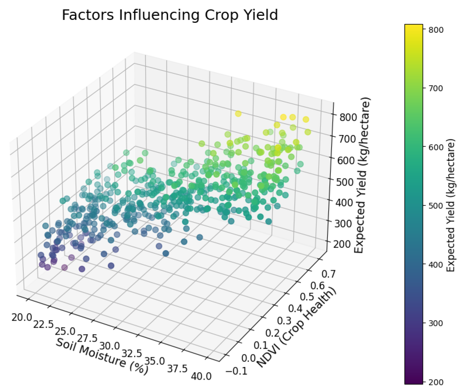
Figure 3 shows a 3D scatter plot examining how soil moisture (%), the NDVI (crop health), and temperature (°C) affect crop production (kg/hectare). The gradient shows yield levels, with darker tones representing greater values. The technical conclusion shows that the NDVI and soil moisture positively affect yield because adequate moisture levels and crop health boost output. The figure also illustrates that temperature excursions from 25 °C reduce yield, emphasizing the need for climatic stability. This visualization quantifies how environmental conditions affect yield, making it essential for agricultural decision making. These correlations help to optimize irrigation, fertilizer, and crop selection for production. This research also helps to design adaptive techniques to reduce crop performance losses from temperature fluctuation. 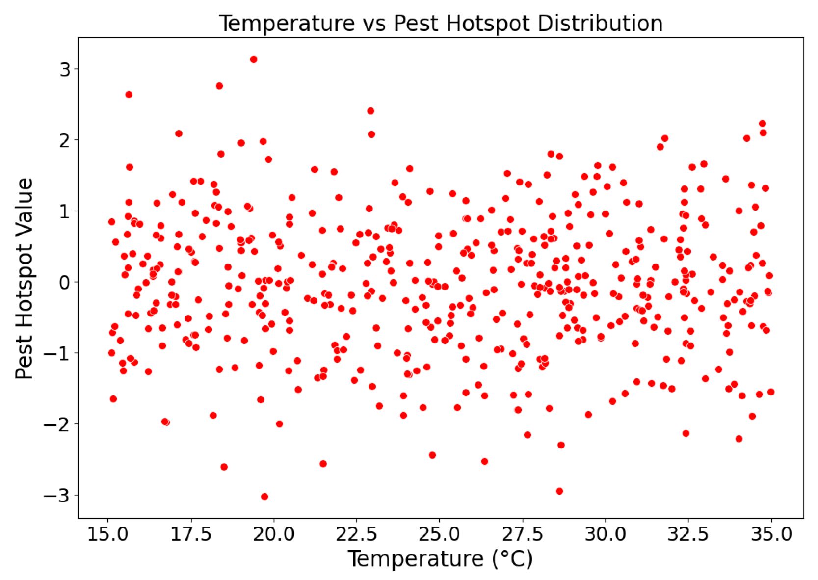Figure 4 shows a scatter plot of the link between temperature (°C) and pest hotspot distribution. Pest activity is more significant in red data points. The technical result shows a modest association between increasing temperatures and pest infestations, demonstrating pest activity during certain temperatures. This graphic helps to explain how temperature changes affect insect behavior. By pinpointing critical times for pesticide application or biological controls, such insights allow for focused pest management. This study also emphasizes the need for environmentally appropriate environments to decrease insect outbreaks. Preventing production losses from insect activity and encouraging sustainable pest control are crucial for precision agriculture. The visualization predicts temperature-induced insect population increases.

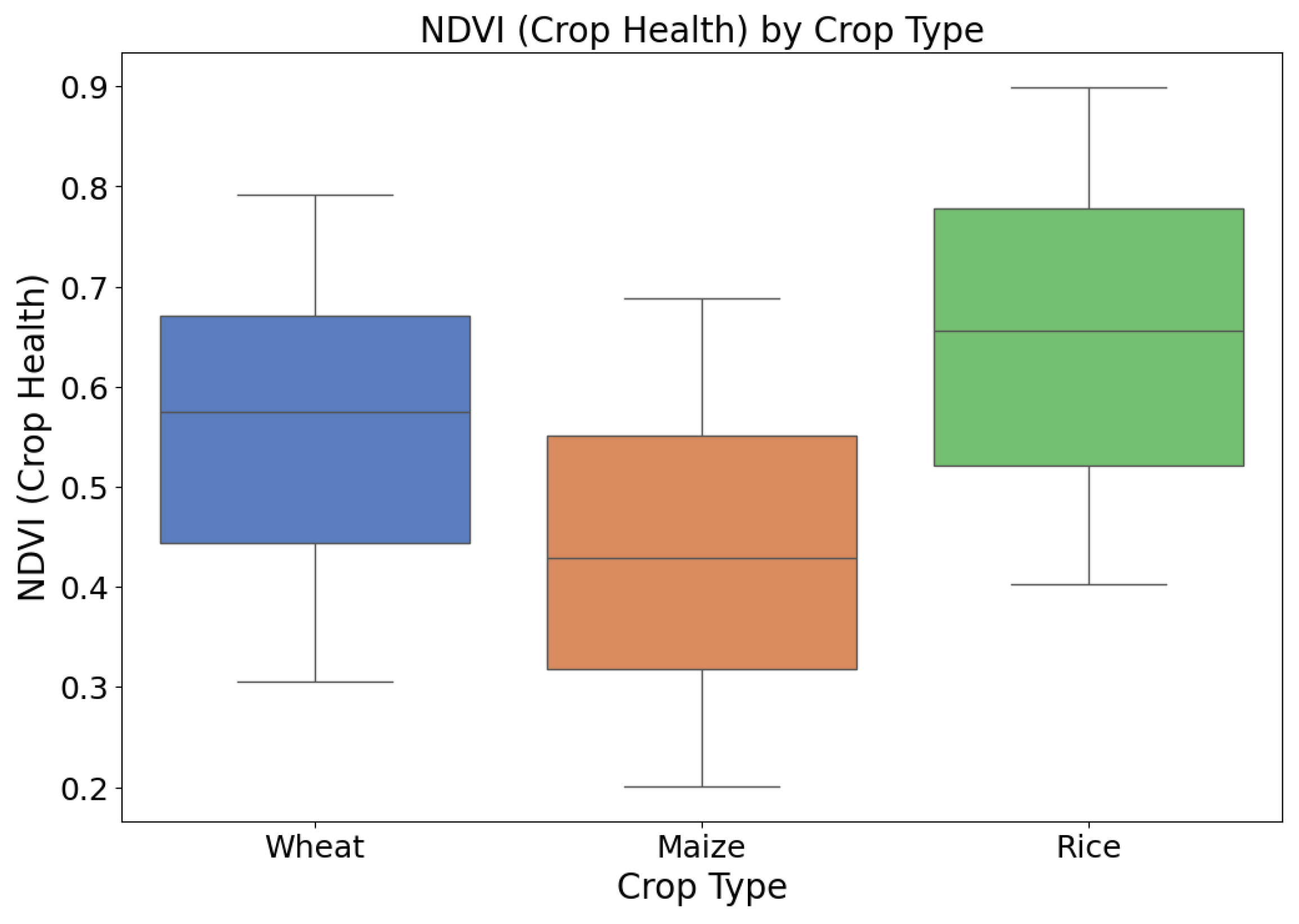
The box plot in Figure 5 displays NDVI (crop health) data for wheat, maize, and rice crops. Rice has higher NDVI readings, indicating crop health, followed by wheat and maize. The technical result shows crop health heterogeneity among crop kinds under comparable environmental conditions. This depiction is essential for crop evaluation and ecological appropriateness. NDVI values show fluctuation for each crop due to nutrient availability, irrigation efficiency, and insect resistance. This figure helps agricultural stakeholders to allocate resources by identifying high-performing crops for specific situations. It also provides a standard for assessing crop health after fertilization, irrigation, and insect management, allowing focused activities to boost agricultural yield.

Figure 6 shows a correlation matrix heatmap for 25 agricultural parameters, such as the NDVI, soil moisture, temperature, and crop production. The technical conclusion shows high positive connections between the NDVI, soil moisture, and vegetation density and moderate negative associations between temperature fluctuation and crop performance. This graphic helps to select predictive modeling features by showing which factors substantially affect crop health and production. Visualization helps researchers to discover redundant or unnecessary information, improving computing efficiency and model correctness. This approach helps to construct precision agricultural machine learning models by identifying feature interdependencies. The figure also helps to plan interventions by highlighting key characteristics like soil moisture and temperature that must be monitored for sustainable farming and yield prediction.

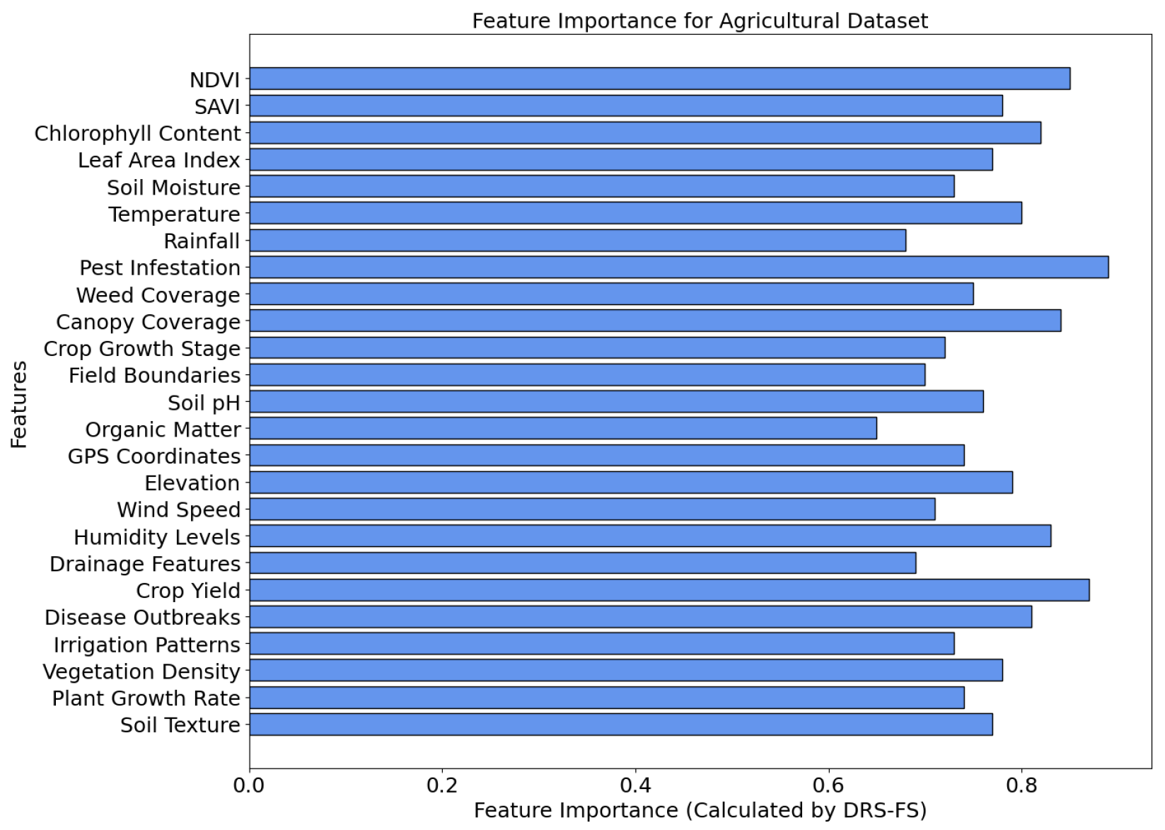
Figure 7 shows DRS-FS-calculated feature significance scores. This bar chart ranks 25 crop management parameters, including the NDVI, pest infestation, soil moisture, and crop growth stage. Pest infestation and the NDVI are essential to agricultural performance. This study illustrates how advanced feature selection techniques like DRS-FS discover important variables while lowering dimensionality. For model optimization, this figure prioritizes essential predictors and reduces computing costs. Practically, the results assist stakeholders in prioritizing prediction accuracy and efficiency variables. Sustainable farming is promoted by targeted analysis, which enhances resource-efficient practices, production estimates, and environmental constraint management. 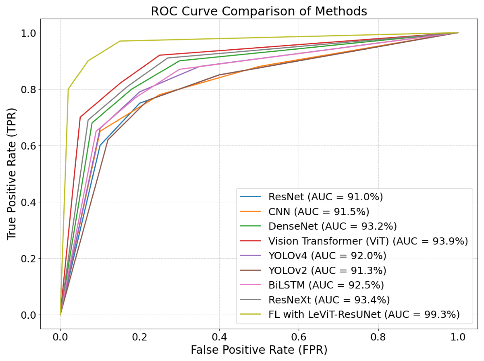Figure 8 displays ROC curves for ResNet, the CNN, DenseNet, ViT, YOLOv4, and the proposed FL with LeViT-ResUNet. Each curve shows the actual positive–false positive trade-off across thresholds. The suggested technique obtains the most excellent AUC of 99.3%, surpassing ResNet (91.0%) and ViT (93.9%). FL with LeViT-ResUNet categorizes agricultural data more correctly and robustly, as this technical conclusion shows. The ROC analysis shows that the model can handle unbalanced datasets, reduce misclassification, and provide accurate pest identification, crop health assessment, and yield predictions. The graphic shows that the model works in real-world agricultural situations and offers a high-performance solution for precision agriculture difficulties.

Table 3. Classification results of different techniques.

Techniques	Log-Loss	AUC (%)	Accuracy (%)	Recall (%)	F1-Score (%)	Precision (%)	FRI (%)	F1I (%)	TDC (%)
ResNet [25]	0.219	91.0	90.4	88.9	88.7	89.5	84.2	73.4	87.3
CNN [11]	0.209	91.5	91.6	89.7	89.8	90.3	85.5	74.8	88.1
DenseNet [15,29]	0.193	93.2	92.8	91.2	91.3	92.1	87.4	77.1	89.0
Vision Transformer (ViT) [16]	0.189	93.9	93.5	92.4	92.5	93.2	88.9	78.2	90.6
YOLOv4 [17]	0.201	92.0	91.9	90.2	90.4	91.5	86.1	75.6	88.7
YOLOv2 [18]	0.216	91.3	91.1	89.4	89.6	90.7	85.2	74.3	87.9
BiLSTM [19]	0.204	92.5	92.0	90.5	90.1	91.8	85.8	75.9	88.5
ResNeXt [27]	0.198	93.4	93.0	91.6	91.7	92.3	87.0	76.8	89.8
LeViT-ResUNet	0.058	99.3	98.9	98.7	98.5	98.8	97.9	93.4	97.5

evaluates machine learning and deep learning strategies for agricultural surveillance. This table compares LeViT-ResUNet with ResNet, the CNN, DenseNet, ViT, YOLO, BiLSTM, ResNeXt, and federated learning. Additionally, it incorporates recent hybrid models such as aKNCN + ELM + mBOA, EBWO-HDLID, Xception + DenseNet-121 fusion, BMA ensemble, MA-CNN-LSTM + AMTBO, and ARIMA-Kalman + SVR-NAR. This comparison shows how well the agricultural data that UAVs gather are examined. Classification accuracy, recall, precision, and other metrics are all outperformed by FL with LeViT-ResUNet compared to conventional models. Regarding feature responsiveness and temporal consistency—two crucial aspects of precision agriculture—the suggested solution outperforms ResNet and DenseNet. The FL’s adaptability, consistency, and flexibility are part of the exhibit with LeViT-ResUNet. Its ability to improve crop health monitoring and output prediction makes it ideal for widespread agricultural deployment.

To demonstrate the efficacy and benefits of our suggested FL-LeViT-ResUNet compared to traditional federated CNN designs,

Table 4. Comparative summary of standard FL-CNN vs. proposed FL-LeViT-ResUNet.

Aspect	Standard FL-CNN	FL-LeViT-ResUNet
Feature Encoding	Spatial, dense	Sparse + attention-aware
Local Data Leakage Risk	Higher	Lower (sparse features + masking)
Communication Overhead	Moderate to High	Low (optimized via DRS-FS)
Cross-client Adaptability	Limited	High (client-level feature refinement)
Execution Time per Round	11–14 s	8.5 s
AUC (6 clients)	93–95%	99.3%

presents a comparison overview of important FL performance metrics.

Table 5. Federated learning classification results with multiple clients.

Model	Iteration	Client	Accuracy (%)	Precision (%)	Recall (%)	F1 Score (%)	Loss
ResNet [25]	1	First Client	89.8	88.4	88.9	88.6	0.217
		Second Client	90.1	88.6	89.2	88.9	0.216
		Third Client	90.4	88.7	89.5	89.1	0.215
		Fourth Client	90.5	89.0	89.7	89.3	0.214
		Fifth Client	90.6	89.2	89.8	89.5	0.213
	50	Sixth Client	90.8	89.3	89.9	89.6	0.212
CNN [11]	1	First Client	91.4	90.2	90.5	90.3	0.208
		Second Client	91.6	90.4	90.7	90.5	0.207
		Third Client	91.8	90.6	90.8	90.7	0.206
		Fourth Client	91.9	90.8	91.0	90.9	0.205
		Fifth Client	92.0	90.9	91.1	91.0	0.204
	50	Sixth Client	92.2	91.0	91.3	91.2	0.203
DenseNet [15,29]	1	First Client	92.5	91.0	91.3	91.1	0.194
		Second Client	92.7	91.2	91.5	91.3	0.193
		Third Client	92.9	91.3	91.7	91.5	0.192
		Fourth Client	93.0	91.5	91.8	91.7	0.191
		Fifth Client	93.2	91.7	91.9	91.8	0.190
	50	Sixth Client	93.4	91.8	92.1	91.9	0.189
Vision Transformer (ViT) [16]	1	First Client	93.1	92.0	92.3	92.2	0.190
		Second Client	93.3	92.2	92.5	92.4	0.189
		Third Client	93.5	92.3	92.6	92.5	0.188
		Fourth Client	93.6	92.5	92.8	92.7	0.187
		Fifth Client	93.8	92.6	92.9	92.8	0.186
	50	Sixth Client	94.0	92.8	93.1	93.0	0.185
YOLOv4 [17]	1	First Client	91.7	90.5	90.7	90.6	0.202
		Second Client	91.9	90.7	90.9	90.8	0.201
		Third Client	92.1	90.8	91.1	91.0	0.200
		Fourth Client	92.2	91.0	91.2	91.1	0.199
		Fifth Client	92.4	91.1	91.4	91.3	0.198
	50	Sixth Client	92.6	91.2	91.5	91.4	0.197
aKNCN + ELM + mBOA [52]	1	First Client	93.2	92.4	92.7	92.5	0.181
		Second Client	93.6	92.8	93.0	92.9	0.178
		Third Client	93.9	93.1	93.3	93.2	0.176
		Fourth Client	94.0	93.2	93.4	93.3	0.175
		Fifth Client	94.1	93.3	93.5	93.4	0.174
	50	Sixth Client	94.2	93.4	93.6	93.5	0.173
EBWO-HDLID [53]	1	First Client	93.3	92.5	92.8	92.6	0.178
		Second Client	93.7	92.9	93.1	93.0	0.174
		Third Client	94.0	93.2	93.4	93.3	0.171
		Fourth Client	94.2	93.3	93.6	93.4	0.169
		Fifth Client	94.4	93.5	93.7	93.6	0.168
	50	Sixth Client	94.5	93.7	93.9	93.8	0.167
Xception + DenseNet-121 [54]	1	First Client	93.6	92.8	93.0	92.9	0.172
		Second Client	94.0	93.2	93.4	93.3	0.168
		Third Client	94.3	93.5	93.6	93.6	0.165
		Fourth Client	94.5	93.7	93.8	93.8	0.163
		Fifth Client	94.6	93.8	93.9	93.9	0.162
	50	Sixth Client	94.8	94.0	94.2	94.1	0.160
BMA Ensemble (LSTM, SVR, etc.) [55]	1	First Client	94.2	93.4	93.6	93.5	0.164
		Second Client	94.4	93.6	93.8	93.7	0.162
		Third Client	94.7	93.8	94.0	93.9	0.160
		Fourth Client	94.9	94.0	94.2	94.1	0.158
		Fifth Client	95.0	94.2	94.4	94.3	0.157
	50	Sixth Client	95.1	94.4	94.6	94.5	0.156
MA-CNN-LSTM + AMTBO [56]	1	First Client	95.0	94.1	94.3	94.2	0.155
		Second Client	95.3	94.4	94.5	94.4	0.152
		Third Client	95.5	94.6	94.7	94.6	0.150
		Fourth Client	95.6	94.7	94.9	94.8	0.149
		Fifth Client	95.7	94.8	95.0	94.9	0.148
	50	Sixth Client	95.8	94.9	95.1	95.0	0.147
ARIMA-Kalman + SVR-NAR [57]	1	First Client	95.4	94.5	94.6	94.5	0.151
		Second Client	95.6	94.7	94.8	94.7	0.149
		Third Client	95.7	94.8	94.9	94.8	0.148
		Fourth Client	95.8	94.9	95.0	94.9	0.147
		Fifth Client	95.9	95.0	95.1	95.0	0.146
	50	Sixth Client	96.0	95.2	95.4	95.3	0.145
LeViT-ResUNet (Proposed)	1	First Client	98.5	98.1	98.3	98.2	0.057
		Second Client	98.6	98.2	98.5	98.4	0.056
		Third Client	98.8	98.3	98.6	98.5	0.055
		Fourth Client	98.9	98.4	98.8	98.7	0.054
		Fifth Client	99.0	98.5	98.9	98.8	0.053
	50	Sixth Client	99.1	98.6	99.0	98.9	0.052

compares federated-learning-based classification results for various clients using ResNet, the CNN, DenseNet, ViT, YOLOv4, and the proposed FL with LeViT-ResUNet. The table displays client-specific accuracy, precision, recall, F1-score, and iteration loss. The results for six clients (CL = 1 to CL = 6) demonstrate performance development from the 1st to the 50th iteration. This table shows the federated learning framework’s flexibility and performance improvement across client datasets. With more iterations and clients, the vision transformer (ViT) and DenseNet can generalize across scattered data. Compared to other techniques, the FL with the LeViT-ResUNet model achieves the best accuracy (99.1%) and lowest loss (0.052) by the 50th iteration for the sixth client. This shows its ability to maximize model performance across diverse datasets via federated learning. Client collaboration improves global model performance when the system collects information from dispersed datasets, as seen in the table. Federated learning protects data, making the technique scalable and ideal for agricultural applications. The investigation shows that the suggested technique makes accurate predictions even in remote and resource-constrained contexts. All models in this table were assessed in a federated learning setup with consistent client involvement and aggregation techniques for fair comparison.

Table 6. Client-wise contribution to global model.

Client (CL)	Data Size (Samples)	Local Accuracy (%)	Gradient Contribution (%)	Update Frequency (Rounds)
1	5200	97.2	21.8	10
2	5000	96.8	21.2	12
3	5100	97.5	22.1	9
4	4800	96.9	20.5	11
5	5500	97.4	22.5	8
6	5000	97.1	21.9	10

shows the client-wise contribution to the global model in the federated learning framework. It shows each client’s data size (in samples), local accuracy during training, gradient contribution to the worldwide model, and update frequency (in rounds). The data size column shows sample distribution among the six clients, allowing the federated learning system to use varied datasets. Client models’ accuracy results vary from 96.8% to 97.5%, demonstrating the effectiveness of local training in delivering high precision overdispersed datasets. Gradient contribution estimates each client’s effect on the global model update, stressing the proportionality of data quantity and training quality. Clients with more enormous datasets, such as Client 5 with 5500 samples, have a somewhat more outstanding gradient contribution (22.5%) than others. Federated learning is collaborative since the update frequency statistic shows the number of client–global server communication cycles. Clients with more excellent update rates (e.g., Client 2 with 12 rounds) actively refine the global model, improving aggregated data generalization. This table shows that all customers contribute equally to model optimization. Federated learning incorporates local updates into a strong global model while protecting data privacy, making it ideal for remote and heterogeneous applications like agricultural monitoring systems.

Client-specific optimization results in a federated learning framework are shown in

Table 7. Client-specific optimization over local training.

CL	Local Training Round	Local Accuracy (%)	Loss	Time Taken (s)
1	5	96.8	0.079	12.5
2	5	96.5	0.082	13.0
3	5	97.0	0.075	11.8
4	5	96.7	0.081	12.3
5	5	97.2	0.076	11.5
6	5	96.9	0.078	12.0

across local training rounds. The table details critical performance data, including client local accuracy, training loss, and training time (in s). Local training iterations are standardized to five rounds for all customers in the “Local Training Round” column. The “Local Accuracy” column shows the efficacy of local training, with values from 96.5% to 97.2%. These high accuracy levels show that each client’s local model captures key data patterns, improving the global model. The "Loss" column shows local training errors. Low loss values, between 0.075 and 0.082, indicate that each client is reducing the training error and that the local optimization process is stable and efficient. The “Time Taken” measure shows the computational overhead of local training, with each client requiring 11.5 to 13 s to complete five cycles. Federated learning systems address computing resources and client data distribution, which affect time. This table highlights all clients’ balanced and efficient contributions to federated learning. The clients keep the federated learning framework scalable and efficient by obtaining high accuracy and low loss in an acceptable time. These findings demonstrate the federated approach’s resilience in dispersed situations where clients work independently yet together to optimize the global model.

Table 8. Feature responsiveness and temporal consistency.

CL	FRI (%)	TDC (%)	Accuracy (%)
1	91.5	95.2	97.2
2	91.0	94.8	96.9
3	92.0	95.5	97.5
4	90.8	94.7	96.8
5	91.8	95.3	98.4
6	91.2	95.0	98.9

evaluates feature responsiveness and temporal consistency for each client in the federated learning framework. In the feature responsiveness index (FRI) range of 90.8% to 92.0%, the model prioritizes relevant characteristics for successful decision making. Temporal dependency consistency (TDC) scores of 94.7% to 95.5% demonstrate the model’s ability to capture time-dependent patterns needed for sequential data jobs. The global model’s accuracy results (96.8% to 98.9%) show its outstanding prediction performance for all customers. Clients with higher FRI and TDC scores have greater accuracy, emphasizing feature prioritization and temporal alignment in federated learning. This table shows that the model performs equally across dispersed clients while responding to feature dependencies and temporal dynamics.

Table 9. Communication overhead analysis.

Round No.	Data Sent to Clients (MB)	Data Received from Clients (MB)	Total Communication (MB)	Latency per Round (ms)
10	25	65	90	140
20	23	62	85	135
30	24	63	87	138
40	22	61	83	132
50	21	60	81	130

analyzes communication overhead in federated learning frameworks throughout training cycles. In the table, data transferred to and received from clients, overall communication volume, and delay per round are assessed. The model optimizes communication as training rounds grow, reducing the client data provided and received. Communication overhead decreases from 90 MB at round 10 to 81 MB at round 50. This decrease shows the framework’s ability to balance model updates and communication burden. Later rounds had 130 ms latency, down from 140 ms before. The federated learning setup’s efficient communication protocols and aggregation algorithms enable real-time performance in dispersed situations.

Table 10. Execution time comparison of models.

Model	Total Rounds	Execution Time per Round (s)	Total Execution Time (s)
ResNet [25]	30	12.5	375
CNN [11]	30	11.8	354
DenseNet [15,29]	30	13.2	396
Vision Transformer (ViT) [16]	30	14.0	420
YOLOv4 [17]	30	12.3	369
YOLOv2 [18]	30	12.0	360
aKNCN + ELM + mBOA [52]	30	11.5	345
EBWO-HDLID [53]	30	12.6	378
Xception + DenseNet-121 [54]	30	13.0	390
BMA Ensemble (LSTM, SVR, etc.) [55]	30	13.8	414
MA-CNN-LSTM + AMTBO [56]	30	12.9	387
ARIMA-Kalman + SVR-NAR [57]	30	13.6	408
LeViT-ResUNet	30	8.5	255

compares the computational efficiency of different models across 30 training cycles. The table shows that the federated learning (FL) model, coupled with LeViT-ResUNet, has the lowest execution time per round (8.5 s) and overall (255 s). The lightweight LeViT-ResUNet design minimizes computational and communication overhead for federated learning environments, resulting in efficiency. Traditional models like DenseNet, the vision transformer (ViT), and ResNet take 375–420 s to execute. The computational complexity and resource requirements of processing massive agricultural datasets have increased. The suggested FL-based architecture is more efficient than YOLOv4 and YOLOv2, which have reasonable execution times. The findings demonstrate the benefits of lightweight deep learning models with federated learning. The suggested solution minimizes computing costs while retaining accuracy by dividing the training process over numerous clients and using an efficient architecture. This efficiency makes the FL with the LeViT-ResUNet model ideal for real-time agricultural monitoring applications that need fast processing and low latency for decision making. This table evaluated all models under a federated learning setup with consistent client participation and aggregation strategy for a fair comparison.

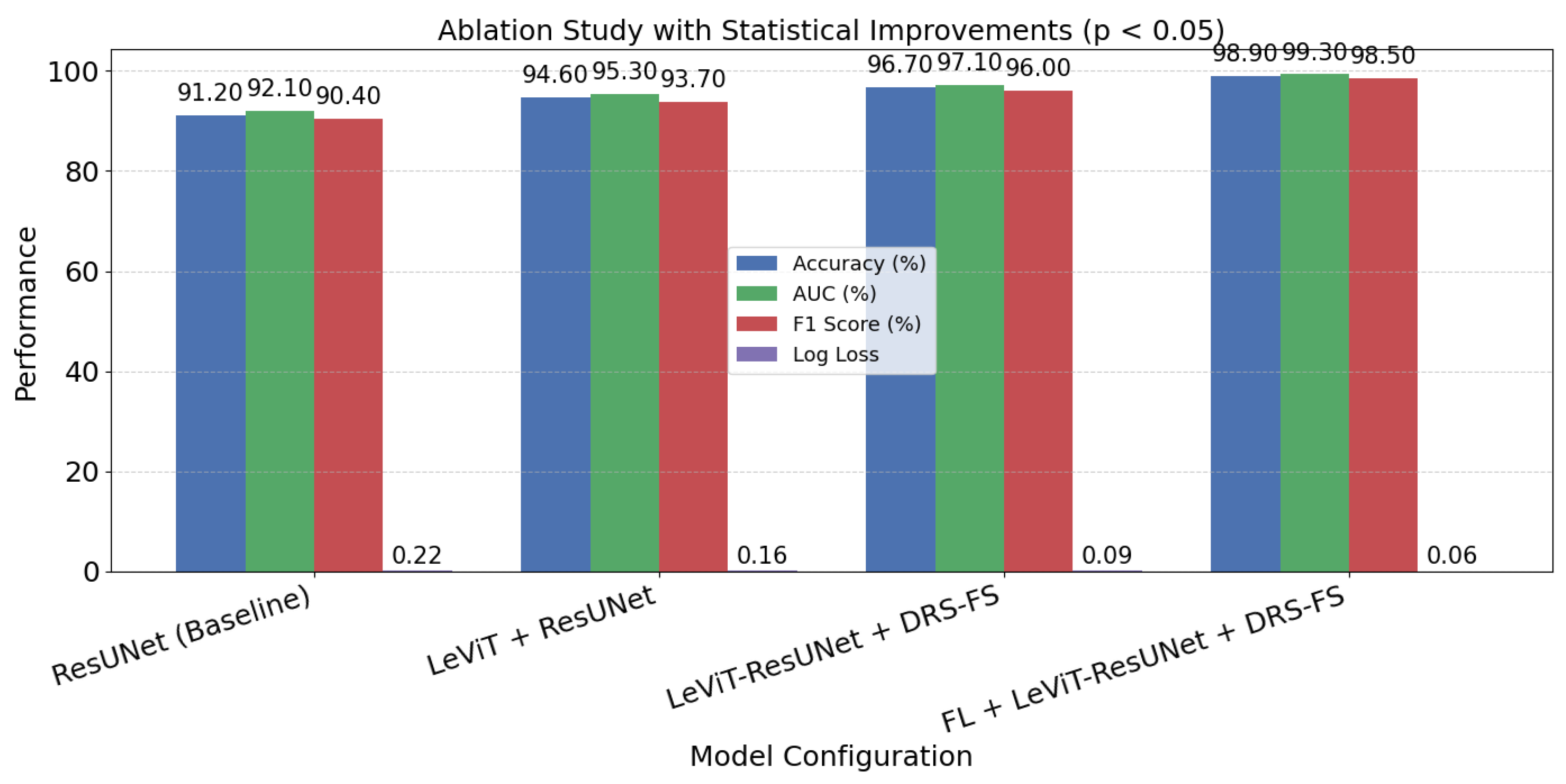
The results in

Table 11. Ablation study of individual model components.

Configuration	Accuracy (%)	AUC (%)	F1 Score (%)	Log Loss
Baseline ResUNet	91.2	92.1	90.4	0.218
LeViT + ResUNet	94.6	95.3	93.7	0.157
LeViT-ResUNet + DRS-FS	96.7	97.1	96.0	0.094
FL + LeViT-ResUNet + DRS-FS	98.9	99.3	98.5	0.058

and Figure 9 demonstrate the individual and collective value of each integrated component within the proposed architecture, and the statistical improvements across configurations are significant (p < 0.05) as validated using paired Student’s t-tests, confirming the effectiveness of each integrated component. Starting from the baseline ResUNet, which provides foundational pixel-level segmentation, the addition of the LeViT significantly improves performance by introducing attention-driven, spatially aware feature extraction, resulting in a 3.4% gain in accuracy and a 0.061 reduction in log-loss. When the dynamic relevance and sparsity-based feature selector (DRS-FS) is added, the model further benefits from targeted feature prioritization, improving generalization and interpretability. This is evident with a jump in accuracy from 94.6% to 96.7% and a log-loss drop from 0.157 to 0.094. Finally, integrating federated learning (FL) enables decentralized model training across geographically distributed datasets, preserving data privacy and enhancing regional variability adaptability. This results in the highest observed performance, with an accuracy of 98.9% and the lowest log-loss of 0.058. Overall, the full model achieves a substantial 7.7% increase in classification accuracy and a 0.16 reduction in log-loss compared to the baseline, confirming the necessity and synergistic impact of each component in delivering a robust, privacy-preserving, and high-performing precision agriculture solution.

Table 12. Statistical analysis comparison.

Classifier	ANOVA	Kolmogorov–Smirnov	Student’s	Chi-Squared	Kendall’s	Spearman’s	t-Test	Mann–Whitney	Paired Student’s	Pearson’s	Wilcoxon
ResNet [25]	2.985	3.020	2.109	2.715	3.410	0.038	2.408	2.410	2.004	0.027	3.145
CNN [11]	3.067	3.198	2.230	2.821	3.562	0.045	2.599	2.482	2.129	0.032	3.198
DenseNet [15,29]	2.798	2.904	2.015	2.536	3.203	0.029	2.304	2.270	1.902	0.022	2.987
Vision Transformer (ViT) [16]	2.750	2.891	1.968	2.480	3.105	0.025	2.107	2.183	1.850	0.019	2.891
YOLOv4 [17]	2.892	3.025	2.111	2.620	3.210	0.033	2.501	2.311	2.000	0.025	3.025
YOLOv2 [18]	3.015	3.102	2.230	2.743	3.335	0.037	2.589	2.452	2.124	0.028	3.102
BiLSTM [19]	3.060	3.134	2.269	2.782	3.367	0.040	2.701	2.491	2.167	0.030	3.134
ResNeXt [27]	2.701	2.876	1.946	2.448	3.012	0.022	2.201	2.134	1.829	0.017	2.876
LeViT-ResUNet	2.590	2.745	1.822	2.302	2.902	0.012	1.904	2.013	1.708	0.009	2.745

shows that federated learning (FL) using the LeViT-ResUNet model excels in several metrics, such as Spearman’s, Pearson’s, Wilcoxon, Kendall’s, ANOVA, and others. The model’s low statistical error values demonstrate its generalization ability across varied datasets, assuring stable performance and low variability. The model’s unusual architecture—combining LeViT’s lightweight transformer-based feature extraction with ResUNet’s exact pixel-level segmentation—explains its effectiveness. Federated learning uses decentralized, heterogeneous client data to reduce overfitting and improve consistency, enhancing flexibility. FL with LeViT-ResUNet outperforms ResNet, the CNN, and DenseNet in statistical reliability. Its stability in storing complicated agricultural data and low error levels across all tests make it ideal for precision agriculture applications.

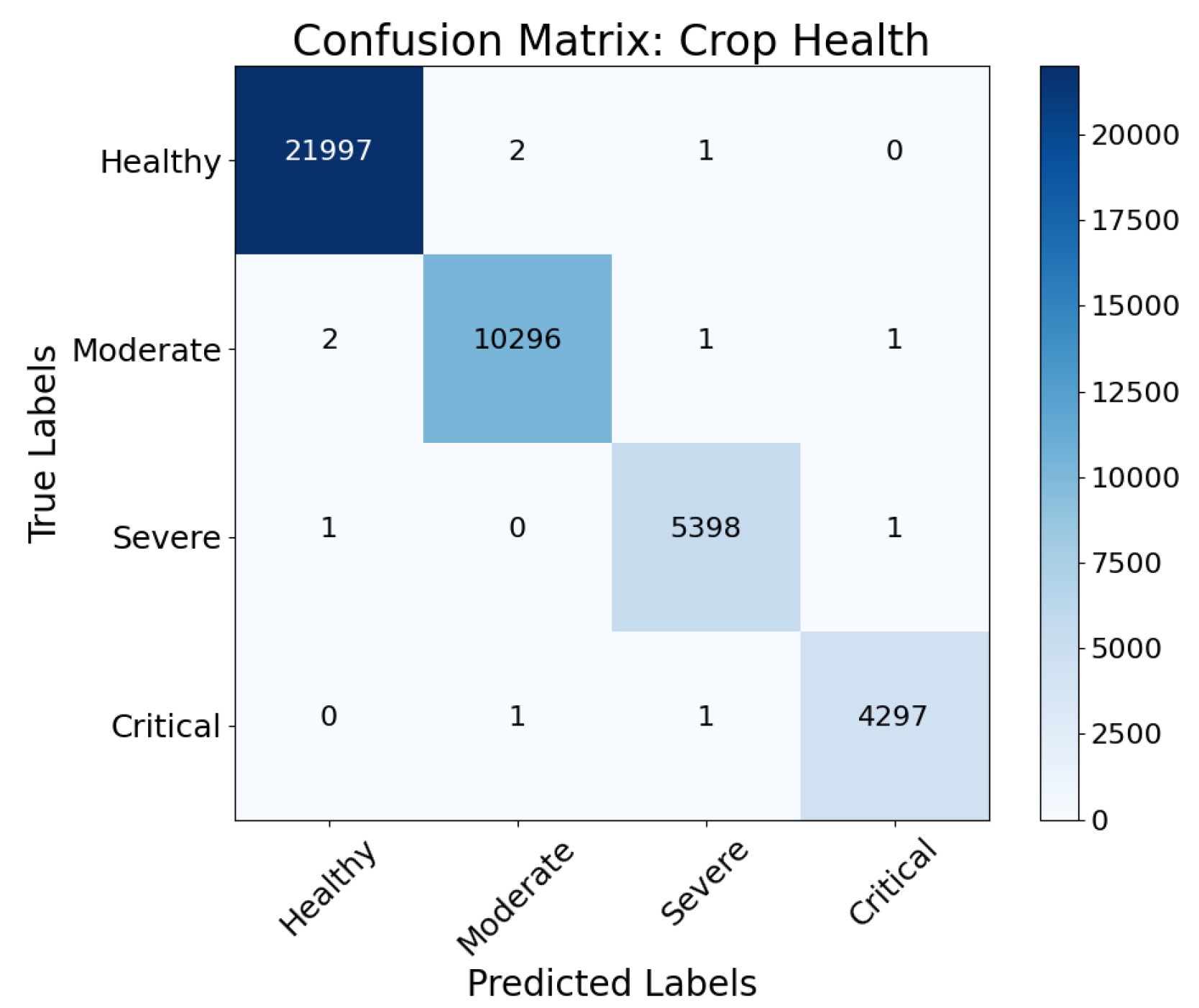
The confusion matrix for crop health classification (Figure 10) assesses predictions for four categories: healthy, moderate, severe, and critical. High diagonal dominance reflects the model’s accurate categorization with minimal false positives and negatives. Near-perfect accuracy allows the model to identify serious crop health issues in the “Healthy” and “Critical” categories. This technical result reveals that the proposed FL with LeViT-ResUNet can properly assess crop health for resource allocation and early response. Early crop stress diagnosis, risk minimization, and production optimization are possible with accurate classification. Real-world agriculture requires precise crop health evaluation for sustainable and practical farming. Hence, the model’s results justify its implementation. 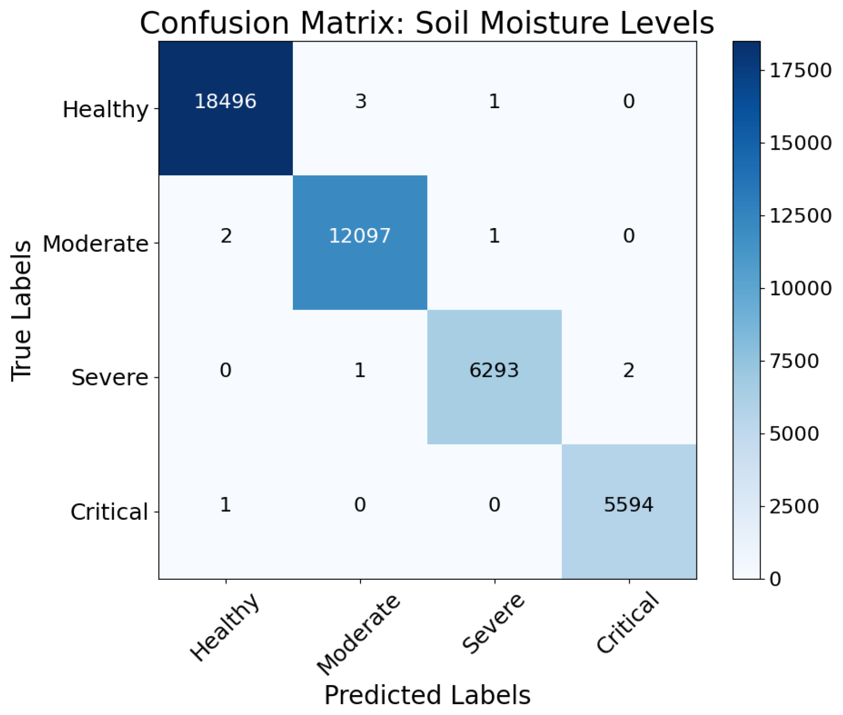Figure 11 shows the confusion matrix for soil moisture classification: healthy, moderate, severe, and critical. The model’s diagonal dominance indicates excellent accuracy and few misclassifications. This technical result confirms the model’s soil moisture accuracy, which optimizes irrigation. Correct soil moisture categorization saves water, reduces resource waste, and prevents crop damage from over- or under-irrigation. This proves that FL with LeViT-ResUNet can solve precision agricultural water management problems. The approach helps farmers to save water, preserve crop health, and conduct sustainable agriculture by delivering soil moisture insights. 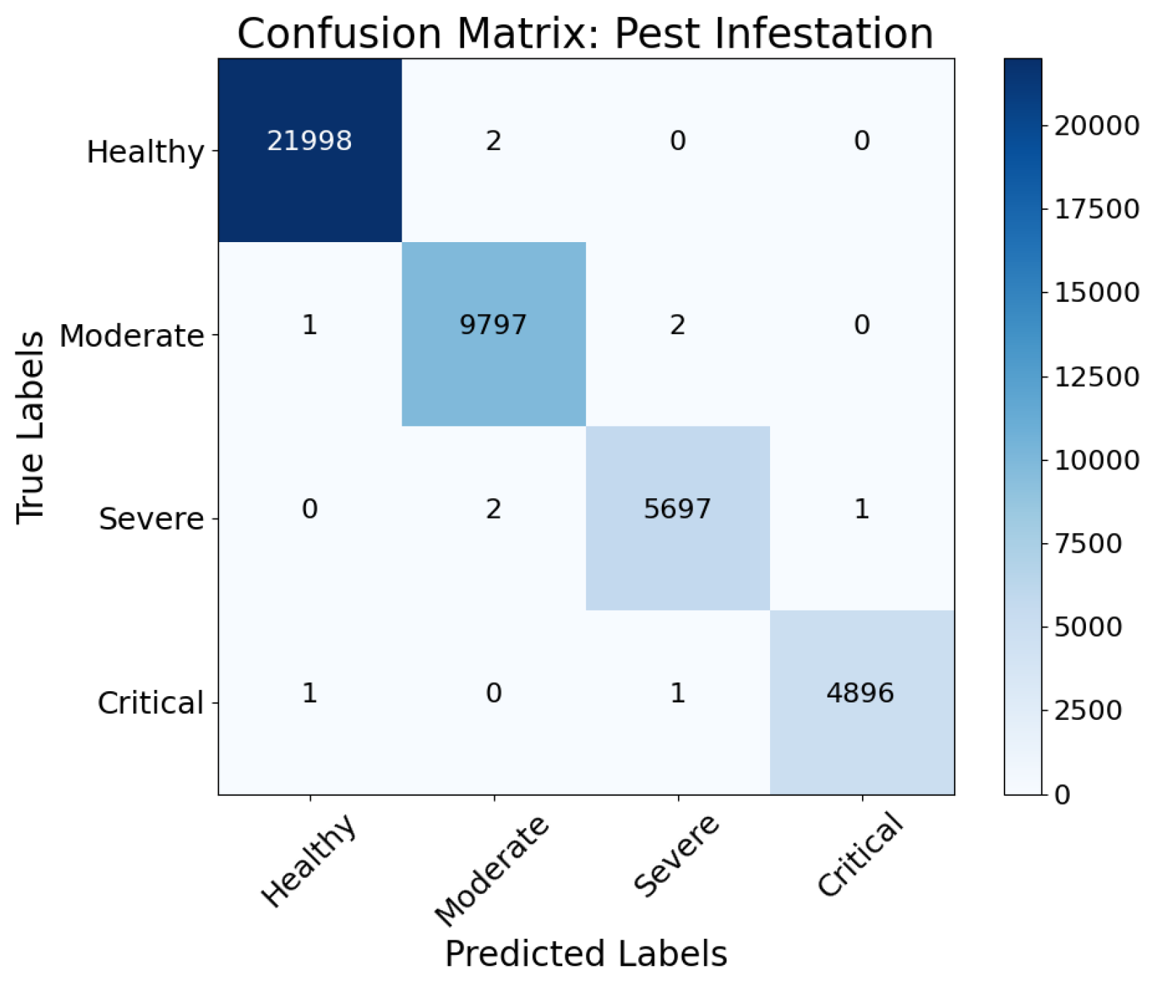Figure 12 shows the confusion matrix for pest infestation categorization, categorized as healthy, moderate, severe, and critical. The model accurately identifies pest-affected areas with few false positives and negatives. This technical result shows that FL with LeViT-ResUNet can accurately identify pest hotspots for timely interventions and targeted pest management. Accurate pest infestation categorization improves crop quality and ecological balance by reducing pesticide use and environmental consequences. Precision agriculture requires accurate pest monitoring for sustainability and production, as seen in the figure. 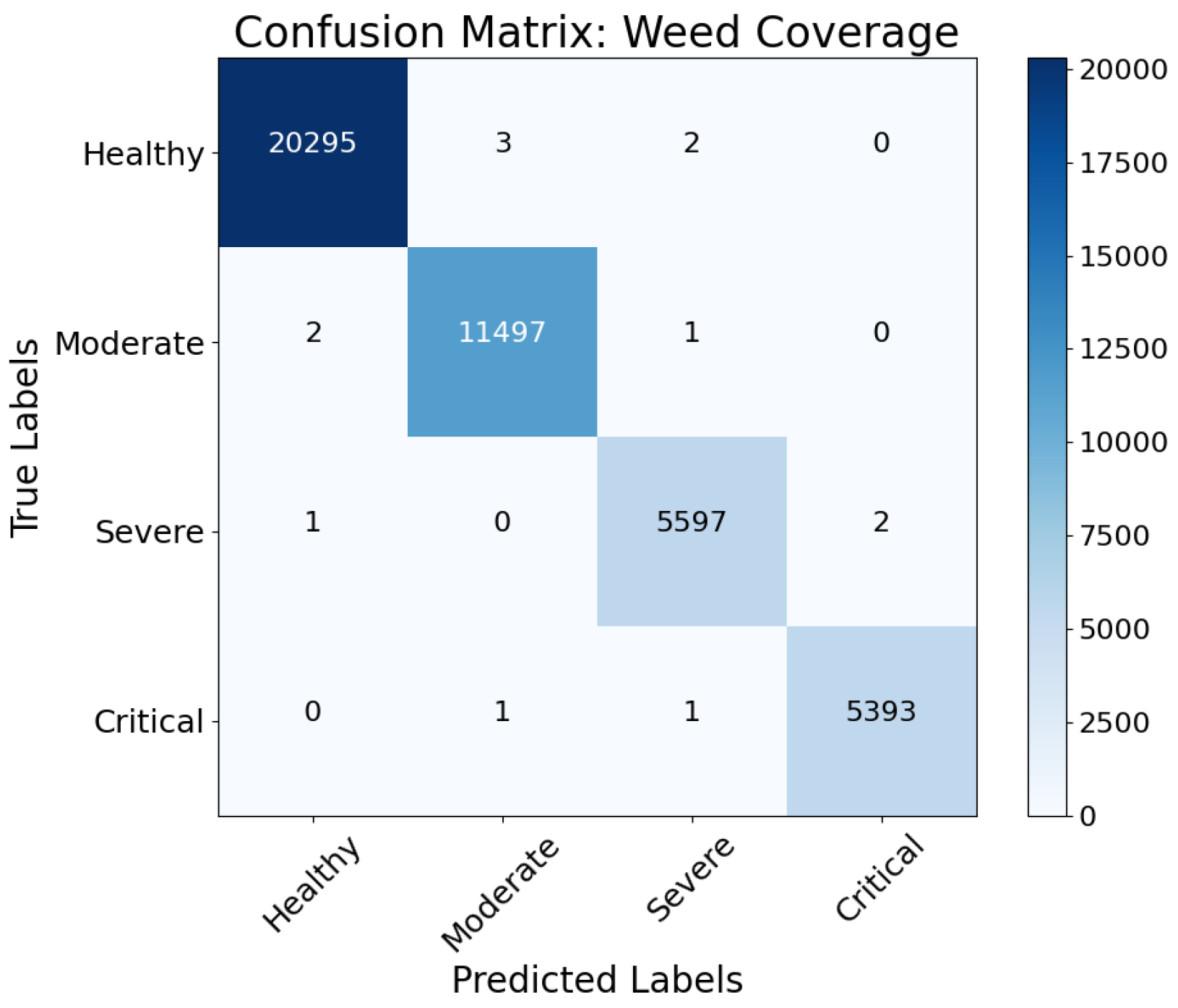Figure 13 illustrates the confusion matrix for weed coverage categorization, divided into four categories: healthy, moderate, severe, and critical. Strong diagonal dominance and low misclassification rates demonstrate the FL with the LeViT-ResUNet model’s correctness. This technical result shows that the model can accurately identify weed-affected regions for herbicide treatment. Correct weed categorization optimizes crop development, reduces resource waste, and boosts production. The findings confirm the model’s use in real-world farming, where timely and accurate weed removal is crucial for crop health and production.

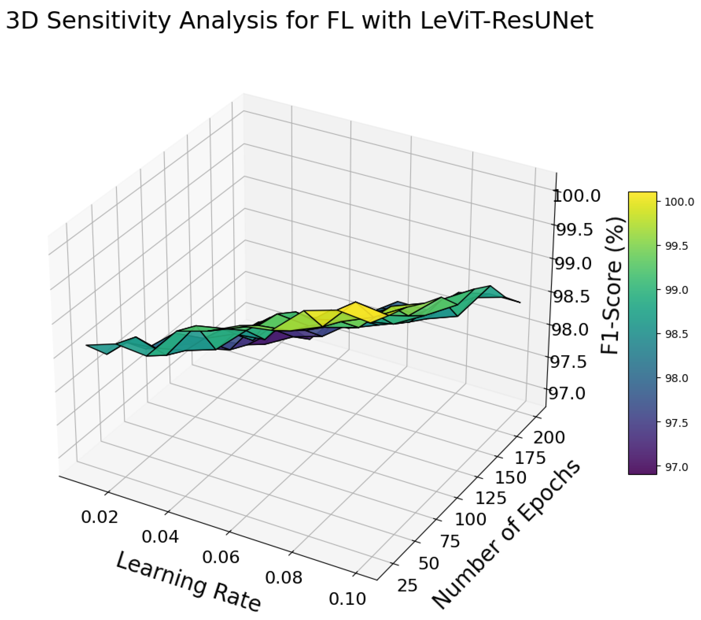
The 3D sensitivity study in Figure 14 illustrates the correlation between learning rate, epochs, and F1-scores in the FL with the LeViT-ResUNet model. The figure shows that F1-scores improve with the best learning rate (∼$0.05$) and sufficient epochs (∼100). This study allows hyperparameter adjustment to optimize model performance and reduce computing costs. Federated learning systems must combine efficiency and accuracy with distributed environment restrictions. Therefore, such insights are essential. The findings confirm the model’s flexibility across parameter configurations, bolstering its precision agricultural resilience.

This study found that FL with the LeViT-ResUNet system works well in most agricultural settings but degrades under challenging circumstances. The algorithm performs poorly in extensive leaf overlap, when numerous plant layers conceal insect or weed patterns, reducing pixel-level segmentation accuracy. Even after preprocessing, cloud cover and uneven illumination in drone footage may distort spectral images. In severe weather conditions like high wind speeds or partial blockage from rain or dust, the model’s ability to detect crop health indicators like the NDVI and insect hotspots decreases. Motion blur, picture artifacts, and ambient noise impact feature spatial coherence. Due to low aerial characteristics, some crop kinds with comparable spectral profiles (e.g., maize vs. sorghum in early development stages) are easier to misclassify. Our preparation workflow uses spatial filtering, temporal alignment, and the DRS-FS feature selector to remove redundant or noisy data. Under high noise or partial occlusions, the model may show a little performance loss (2-4% accuracy reduction in impacted areas). Future research objectives include integrating adaptive attention processes or multi-view fusion procedures to improve resilience under occlusion, illumination change, and visually confusing crop settings.

5. Conclusions

This work proposed the LeViT-ResUNet system with federated learning to handle precision agricultural monitoring concerns, such as crop health assessment, insect infestation detection, and soil moisture categorization. Drone-captured pictures and ground-based IoT data were transformed into tabular datasets for analysis by the system. The suggested model outperformed state-of-the-art approaches, with an excellent AUC of 99.3% and higher classification accuracy in diverse agricultural tasks. The model achieved computational efficiency and strong predictive performance by integrating lightweight feature extraction with LeViT and ResUNet pixel-level segmentation. According to simulations, pests and environmental stressors, such as soil moisture and temperature fluctuation, were the main variables affecting crop health and yield. Specific pest hotspots indicated the need for tailored efforts to reduce hazards. Federated learning protected data privacy and enabled model generalization over remote and heterogeneous datasets, accommodating varied environmental conditions and crop varieties. This makes the strategy ideal for large-scale, dispersed agriculture. The research has limits despite its success. Drone data and IoT devices may be challenging to use in low-technology areas. Data quality and consistency, which might change owing to environmental variables or device calibration, affect system performance. Although the proposed LeViT-ResUNet architecture is lightweight and optimized for low-resource environments, real-time federated deployment across large-scale agricultural zones may still be limited due to infrastructure constraints such as connectivity, power, or hardware availability in rural settings.

The system can be improved by adding multimodal data like weather predictions, satellite imaging, and socioeconomic variables to improve prediction. Optimizing the federated learning system for scalability and efficiency in large-scale deployments and investigating sophisticated privacy-preserving techniques will increase its usefulness. Adding advanced farmer decision-support technologies like yield forecasts and intervention suggestion systems might help to improve global agriculture practices. Despite the system’s generally excellent performance, it could suffer when faced with heavy vegetation, cloud cover, or harsh weather. Strengthening resistance to occlusion and noise will be the primary goal of future upgrades, especially for use in visually challenging or low-light agricultural environments.

References

1. Getahun, S.; Kefale, H.; Gelaye, Y. Application of precision agriculture technologies for sustainable crop production and environmental sustainability: A systematic review. Sci. World J. 2024, 2024, 2126734. [Google Scholar] [CrossRef]
2. Borsetta, G.; Zovi, A.; Vittori, S. Long-Term Frameworks for Food Security and Sustainability Through Climate-Smart Interconnected Agrifood Systems. Sci 2025, 7, 15. [Google Scholar] [CrossRef]
3. Khatri, P.; Kumar, P.; Shakya, K.S.; Kirlas, M.C.; Tiwari, K.K. Understanding the intertwined nature of rising multiple risks in modern agriculture and food system. Environ. Dev. Sustain. 2024, 26, 24107–24150. [Google Scholar] [CrossRef]
4. Ndlovu, H.S.; Odindi, J.; Sibanda, M.; Mutanga, O. A systematic review on the application of UAV-based thermal remote sensing for assessing and monitoring crop water status in crop farming systems. Int. J. Remote Sens. 2024, 45, 4923–4960. [Google Scholar] [CrossRef]
5. Zhou, Y.; Zhou, H.; Chen, Y. An Automated Phenotyping Method for Chinese Cymbidium Seedlings Based on 3D Point Cloud. Plant Methods 2024, 20, 151. [Google Scholar] [CrossRef] [PubMed]
6. Chowdhury, M.; Anand, R.; Dhar, T.; Kurmi, R.; Sahni, R.K.; Kushwah, A. Digital insights into plant health: Exploring vegetation indices through computer vision. In Applications of Computer Vision and Drone Technology in Agriculture 4.0; Springer Nature: Singapore, 2024; pp. 7–30. [Google Scholar]
7. Duan, H.; Li, Y.; Yuan, Y. A study on the long-term impact of crop rotation on soil health driven by big data. Geogr. Res. Bull. 2024, 3, 348–369. [Google Scholar]
8. Amulothu, D.V.R.T.; Rodge, R.R.; Hasan, W.; Gupta, S. Machine Learning for Pest and Disease Detection in Crops. In Agriculture 4.0; CRC Press: Boca Raton, FL, USA, 2024; pp. 111–132. [Google Scholar]
9. Usigbe, M.J.; Asem-Hiablie, S.; Uyeh, D.D.; Iyiola, O.; Park, T.; Mallipeddi, R. Enhancing resilience in agricultural production systems with AI-based technologies. Environ. Dev. Sustain. 2024, 26, 21955–21983. [Google Scholar] [CrossRef]
10. Kariyanna, B.; Sowjanya, M. Unravelling the use of artificial intelligence in management of insect pests. Smart Agric. Technol. 2024, 8, 100517. [Google Scholar] [CrossRef]
11. Kaya, Y.; Gürsoy, E. A novel multi-head CNN design to identify plant diseases using the fusion of RGB images. Ecol. Inform. 2023, 75, 101998. [Google Scholar] [CrossRef]
12. Bera, A.; Krejcar, O.; Bhattacharjee, D. Rafa-net: Region attention network for food items and agricultural stress recognition. IEEE Trans. AgriFood Electron. 2024; Early Access. [Google Scholar] [CrossRef]
13. Jiang, C.; Wang, Y.; Yang, Z.; Zhao, Y. Do Adaptive Policy Adjustments Deliver Ecosystem-Agriculture-Economy Co-Benefits in Land Degradation Neutrality Efforts? Evidence From Southeast Coast of China. Environ. Monit. Assess. 2023, 195, 1215. [Google Scholar] [CrossRef]
14. Kempelis, A.; Polaka, I.; Romanovs, A.; Patlins, A. Computer Vision and Machine Learning-Based Predictive Analysis for Urban Agricultural Systems. Future Internet 2024, 16, 44. [Google Scholar] [CrossRef]
15. Mazumder, M.K.A.; Kabir, M.M.; Rahman, A.; Abdullah-Al-Jubair, M.; Mridha, M.F. DenseNet201Plus: Cost-effective transfer-learning architecture for rapid leaf disease identification with attention mechanisms. Heliyon 2024, 10, 15. [Google Scholar] [CrossRef]
16. Pintus, M.; Colucci, F.; Maggio, F. Emerging Developments in Real-Time Edge AIoT for Agricultural Image Classification. IoT 2025, 6, 13. [Google Scholar] [CrossRef]
17. Sun, J.; Zhou, J.; He, Y.; Jia, H.; Rottok, L.T. Detection of rice panicle density for unmanned harvesters via RP-YOLO. Comput. Electron. Agric. 2024, 226, 109371. [Google Scholar] [CrossRef]
18. Zhang, T.; Zhong, L.; Wu, S.; Han, K.; Peng, B. BCP-YOLO: A Lightweight Industrial Tomato Detection Method for UAV Inspection. In Proceedings of the 2024 7th International Conference on Computer Information Science and Artificial Intelligence, Shaoxing, China, 13–15 September 2024; IEEE: Piscataway, NJ, USA, 2024; pp. 474–480. [Google Scholar]
19. Mahmoud, A.; Mohammed, A.; Khalil, A.A. Time series forecasting of wheat crop productivity in Egypt using deep learning techniques. Int. J. Data Sci. Anal. 2024, 1–16. [Google Scholar] [CrossRef]
20. Cheng, J.; Huang, L.; Tang, B.; Wu, Q.; Wang, M.; Zhang, Z. A Minority Sample Enhanced Sampler for Crop Classification in Unmanned Aerial Vehicle Remote Sensing Images with Class Imbalance. Agriculture 2025, 15, 388. [Google Scholar] [CrossRef]
21. Liu, X.; Gong, H.; Guo, L.; Gu, X.; Zhou, J. A Novel Approach for Maize Straw Type Recognition Based on UAV Imagery Integrating Height, Shape, and Spectral Information. Drones 2025, 9, 125. [Google Scholar] [CrossRef]
22. Gokeda, V.; Yalavarthi, R. Deep Hybrid Model for Pest Detection: IoT-UAV-Based Smart Agriculture System. J. Phytopathol. 2024, 172, e13381. [Google Scholar] [CrossRef]
23. Yin, Y.; Wang, Z.; Zheng, L.; Su, Q.; Guo, Y. Autonomous UAV Navigation with Adaptive Control Based on Deep Reinforcement Learning. Electronics 2024, 13, 2432. [Google Scholar] [CrossRef]
24. Upadhyay, N.; Gupta, N. Detecting fungi-affected multi-crop disease on heterogeneous region dataset using modified ResNeXt approach. Environ. Monit. Assess. 2024, 196, 610. [Google Scholar] [CrossRef]
25. Zhang, L.; Li, C.; Wu, X.; Xiang, H.; Jiao, Y.; Chai, H. BO-CNN-BiLSTM deep learning model integrating multisource remote sensing data for improving winter wheat yield estimation. Front. Plant Sci. 2024, 15, 1500499. [Google Scholar] [CrossRef]
26. Farhansyah, D.A.N.; Al Maki, W.F. Revolutionizing Banana Grading with ResNeXt and SVM: An Automated Approach. In Proceedings of the 2023 11th International Conference on Information and Communication Technology (ICoICT), Melaka, Malaysia, 23–24 August 2023; IEEE: Piscataway, NJ, USA, 2023; pp. 184–189. [Google Scholar]
27. Gibril, M.B.A.; Shafri, H.Z.M.; Shanableh, A.; Al-Ruzouq, R.; bin Hashim, S.J.; Wayayok, A.; Sachit, M.S. Large-scale assessment of date palm plantations based on UAV remote sensing and multiscale vision transformer. Remote Sens. Appl. Soc. Environ. 2024, 34, 101195. [Google Scholar] [CrossRef]
28. Xin, X.; Gong, H.; Hu, R.; Ding, X.; Pang, S.; Che, Y. Intelligent large-scale flue-cured tobacco grading based on deep densely convolutional network. Sci. Rep. 2023, 13, 11119. [Google Scholar] [CrossRef] [PubMed]
29. Luo, J.; Zhao, C.; Chen, Q.; Li, G. Using Deep Belief Network to Construct the Agricultural Information System Based on Internet of Things. J. Supercomput. 2022, 78, 379–405. [Google Scholar] [CrossRef]
30. Aldhahri, E.A.; Almazroi, A.A.; Alkinani, M.H.; Ayub, N.; Alghamdi, E.A.; Janbi, N.F. Smart Farming: Enhancing Urban Agriculture through Predictive Analytics and Resource Optimization. IEEE Access 2025. Early Access. [Google Scholar] [CrossRef]
31. Aldossary, M.; Alharbi, H.A.; Hassan, C.A.U. Internet of Things (IoT)-Enabled Machine Learning Models for Efficient Monitoring of Smart Agriculture. IEEE Access 2024, 12, 75718–75734. [Google Scholar] [CrossRef]
32. Alharbi, H.A.; Aldossary, M. Energy-efficient edge-fog-cloud architecture for IoT-based smart agriculture environment. IEEE Access 2021, 9, 110480–110492. [Google Scholar] [CrossRef]
33. Aldossary, M.; Alzamil, I.; Almutairi, J. Enhanced Intrusion Detection in Drone Networks: A Cross-Layer Convolutional Attention Approach for Drone-to-Drone and Drone-to-Base Station Communications. Drones 2025, 9, 46. [Google Scholar] [CrossRef]
34. Li, W.; Lambert-Garcia, R.; Getley, A.C.M.; Kim, K.; Bhagavath, S.; Majkut, M.; Rack, A.; Lee, P.D. AM-SegNet for additive manufacturing in situ X-ray image segmentation and feature quantification. Virtual Phys. Prototyp. 2024, 19, 2325572. [Google Scholar] [CrossRef]
35. EUROCROP24. Crop Health and Environmental Stress Dataset. Kaggle 2025. Available online: https://doi.org/10.34740/KAGGLE/DSV/10605890 (accessed on 1 February 2025).
36. Greenacre, M.; Groenen, P.J.; Hastie, T.; d’Enza, A.I.; Markos, A.; Tuzhilina, E. Principal component analysis. Nat. Rev. Methods Prim. 2022, 2, 100. [Google Scholar] [CrossRef]
37. Chen, X.; Xie, D.; Zhang, Z.; Sharma, R.P.; Chen, Q.; Liu, Q.; Fu, L. Compatible Biomass Model with Measurement Error Using Airborne LiDAR Data. Remote Sens. 2023, 15, 3546. [Google Scholar] [CrossRef]
38. Ma, X.; Wang, T.; Lu, L.; Huang, H.; Ding, J.; Zhang, F. Developing a 3D Clumping Index Model to Improve Optical Measurement Accuracy of Crop Leaf Area Index. Field Crop. Res. 2022, 275, 108361. [Google Scholar] [CrossRef]
39. Ma, X.; Liu, Y. A Modified Geometrical Optical Model of Row Crops Considering Multiple Scattering Frame. Remote Sens. 2020, 12, 3600. [Google Scholar] [CrossRef]
40. Ma, X.; Ding, J.; Wang, T.; Lu, L.; Sun, H.; Zhang, F.; Nurmemet, I. A Pixel Dichotomy Coupled Linear Kernel-Driven Model for Estimating Fractional Vegetation Cover in Arid Areas From High-Spatial-Resolution Images. IEEE Trans. Geosci. Remote Sens. 2023, 61, 1–15. [Google Scholar] [CrossRef]
41. Zhou, S.; He, Z.; Chen, X.; Chang, W. An Anomaly Detection Method for UAV Based on Wavelet Decomposition and Stacked Denoising Autoencoder. Aerospace 2024, 11, 393. [Google Scholar] [CrossRef]
42. Gkiatis, K.; Garganis, K.; Karanasiou, I.; Chatzisotiriou, A.; Zountsas, B.; Kondylidis, N.; Matsopoulos, G.K. Independent component analysis: A reliable alternative to general linear model for task-based fMRI. Front. Psychiatry 2023, 14, 1214067. [Google Scholar] [CrossRef]
43. Capotondi, A.; Qiu, B. Decadal variability of the Pacific shallow overturning circulation and the role of local wind forcing. J. Clim. 2023, 36, 1001–1015. [Google Scholar] [CrossRef]
44. Zhang, P.; Yin, H.; Tian, Y.; Zhang, X. An adjoint feature-selection-based evolutionary algorithm for sparse large-scale multiobjective optimization. Complex Intell. Syst. 2025, 11, 127. [Google Scholar] [CrossRef]
45. Nismi Mol, E.A.; Santosh Kumar, M.B. Review on knowledge extraction from text and scope in agriculture domain. Artif. Intell. Rev. 2023, 56, 4403–4445. [Google Scholar] [CrossRef]
46. Huo, X.; Sun, G.; Tian, S.; Wang, Y.; Yu, L.; Long, J.; Li, A. HiFuse: Hierarchical multi-scale feature fusion network for medical image classification. Biomed. Signal Process. Control 2024, 87, 105534. [Google Scholar] [CrossRef]
47. Xu, G.; Zhang, X.; He, X.; Wu, X. Levit-Unet: Make faster encoders with transformer for medical image segmentation. In Proceedings of the Chinese Conference on Pattern Recognition and Computer Vision (PRCV), Xiamen, China, 13–15 October 2023; Springer Nature: Singapore, 2023; pp. 42–53. [Google Scholar]
48. Huang, L.; Miron, A.; Hone, K.; Li, Y. Segmenting Medical Images: From UNet to Res-UNet and nnUNet. In Proceedings of the 2024 IEEE 37th International Symposium on Computer-Based Medical Systems (CBMS), Guadalajara, Mexico, 26–28 June 2024; IEEE: Piscataway, NJ, USA, 2024; pp. 483–489. [Google Scholar]
49. Fergus, P.; Chalmers, C. Performance evaluation metrics. In Applied Deep Learning: Tools, Techniques, and Implementation; Springer: Cham, Switzerland, 2022; pp. 115–138. [Google Scholar]
50. Shahid, U.; Ahmed, G.; Siddiqui, S.; Shuja, J.; Balogun, A.O. Latency-Sensitive Function Placement among Heterogeneous Nodes in Serverless Computing. Sensors 2024, 24, 4195. [Google Scholar] [CrossRef] [PubMed]
51. Chen, J.; Wang, J.; Wang, J.; Bai, L. Joint Fairness and Efficiency Optimization for CSMA/CA-Based Multi-User MIMO UAV Ad Hoc Networks. IEEE J. Sel. Top. Signal Process. 2024, 18, 1311–1323. [Google Scholar] [CrossRef]
52. Gupta, A.; Nahar, P. Classification and yield prediction in smart agriculture system using IoT. J. Ambient Intell. Humaniz. Comput. 2023, 14, 10235–10244. [Google Scholar] [CrossRef]
53. Aburasain, R.Y. Enhanced black widow optimization with hybrid deep learning enabled intrusion detection in Internet of Things-based smart farming. IEEE Access 2024, 12, 16621–16631. [Google Scholar] [CrossRef]
54. Mishra, V.; Naik, N.S.; Kumar, S.; Alsamhi, S.H.; Saif, A.; Curry, E. Maize plant disease prediction of UAV images for precision agriculture using fusion of multimodal. In Proceedings of the 2023 3rd International Conference on Computing and Information Technology (ICCIT), Tabuk, Saudi Arabia, 27–28 September 2023; pp. 353–358. [Google Scholar]
55. Sarkar, T.K.; Roy, D.K.; Kang, Y.S.; Jun, S.R.; Park, J.W.; Ryu, C.S. Ensemble of machine learning algorithms for rice grain yield prediction using UAV-based remote sensing. J. Biosyst. Eng. 2024, 49, 1–19. [Google Scholar] [CrossRef]
56. Padmavathi, B.; BhagyaLakshmi, A.; Vishnupriya, G.; Datchanamoorthy, K. IoT-based prediction and classification framework for smart farming using adaptive multi-scale deep networks. Expert Syst. Appl. 2024, 254, 124318. [Google Scholar] [CrossRef]
57. Borrero, J.D.; Borrero-Domínguez, J.D. Enhancing short-term berry yield prediction for small growers using a novel hybrid machine learning model. Horticulturae 2023, 9, 549. [Google Scholar] [CrossRef]
Figure 1. Proposed drone-based agricultural framework.
Agronomy 15 00928 g001
Figure 2. FL-based LeViT-ResUNet architecture.
Agronomy 15 00928 g002
Figure 3. Three-dimensional scatter plot of factors influencing crop yield.
Agronomy 15 00928 g003
Figure 4. Temperature vs. pest hotspot distribution.
Agronomy 15 00928 g004
Figure 5. NDVI (crop health) distribution by crop type.
Agronomy 15 00928 g005
Figure 6. Realistic correlation matrix of agricultural features.
Agronomy 15 00928 g006
Figure 7. Feature importance for agricultural dataset using DRS-FS.
Agronomy 15 00928 g007
Figure 8. ROC curve comparison of methods.
Agronomy 15 00928 g008
Figure 9. Performance comparison of model configurations with and without LeViT, DRS-FS, and federated learning.
Agronomy 15 00928 g009
Figure 10. Crop health classification.
Agronomy 15 00928 g010
Figure 11. Soil moisture level classification.
Agronomy 15 00928 g011
Figure 12. Pest infestation classification.
Agronomy 15 00928 g012
Figure 13. Weed coverage classification.
Agronomy 15 00928 g013
Figure 14. Three-dimensional sensitivity analysis for FL with LeViT-ResUNet.
Agronomy 15 00928 g014