Article

Simulating Pasture Yield Under Alternative Environments and Grazing Management in Wisconsin, USA

by
Elissa Chasen
1,*,
Eric Booth
2 and
Claudio Gratton
1
1
Department of Entomology, University of Wisconsin-Madison, 1575 Linden Dr., 554 Moore Hall, Madison, WI 53706, USA
2
Department of Plant & Agroecosystem Sciences, University of Wisconsin-Madison, 1575 Linder Dr., 562 Moore Hall, Madison, WI 53706, USA
*
Author to whom correspondence should be addressed.
Agronomy 2025, 15(2), 437; https://doi.org/10.3390/agronomy15020437
Submission received: 15 January 2025 / Revised: 4 February 2025 / Accepted: 7 February 2025 / Published: 11 February 2025
(This article belongs to the Section Grassland and Pasture Science)

Abstract

:
Pasture yield is crucial to the economic viability of grass-based livestock enterprises, yet the difficulty in predicting yields under various environmental and management conditions prevents effective planning. We used USDA-SSURGO data to create a random forest model that predicts pasture yield potential based on soil properties for the state of Wisconsin (USA). This model is highly accurate (RMSE = 0.11 tons/acre, or 4% of the average yield), predicting pasture yields in Wisconsin grasslands to range from 1.0 to5.3 tons/acre, with an average yield of 2.6 tons/acre. We then integrated this model with guidelines from a USDA-NRCS grazing planning tool to adjust pasture yield potential for different levels of grazing intensity. The adjustments were multiplied to the random forest model output and ranged from 0.65 for continuously grazed pasture to 1.2 for pastures rotated more than once per day. The model is available to use within an online decision support tool through an R-shiny interface and can be easily replicated for other states in the Midwest US. The tool is easy to use and can support farmer analysis of the costs and benefits of grass-based agriculture.

1. Introduction

Grass-based agricultural systems provide many ecosystem services including biological diversity and improved flood and climate regulation, as well as forage production for livestock agriculture. Additionally, because pasture is a low-cost animal feed, these agricultural systems can economically outperform annual row-crop-based animal operations [1,2,3,4]. However, to be successful in grass-based farming systems, the pasture produced on site must meet herd feeding demand. Therefore, pasture yield prediction is a critical part of farming decisions as it constrains the number of animals that the land can sustain without supplementing animal feed from other sources. A survey of nearly 1000 dairy farmers in the northeastern US revealed that a significant barrier to grass-based agriculture was meeting feeding requirements with pasture [5]. Thus, estimating pasture production is a basis for making informed decisions about herd management for both established grass-based farming operations and for farmers interested in transitioning to grazing.
Existing pasture yield prediction models are not easy to use or easily transferable to the Midwest US region. These models have been developed for more moderate climates such as Australia and New Zealand [6] or Ireland and Central Europe [7]. Additionally, these models are process-based, taking into account plant physiology and phenology [8,9], and require data-intensive calibrations. Even after doing so, the predictions might not be satisfactorily accurate [10]. The authors are not aware of any existing pasture yield models for the Midwest United States.
Models created for cash crops such as maize show that yield is highly variable and dependent on a range of variables including soil properties, management, and weather [11,12,13]. In some years, studies show that soil properties alone can explain up to 85% of the yield variability in a given location (mean 46%, range 0–85%) [14]. The combination of the increasing availability of large spatial datasets with complex, non-linear interactions between variables has led to an increasing use of machine learning algorithms to predict crop yields [15,16]. In these analyses, soil type and related variables are the most used predictors in machine learning algorithms for predicting yield [16], followed by climatic variables.
For pastures, another significant variable that influences productivity is grazing management [17]. In the subhumid grasslands of the upper Midwest, United States, several studies show that rotationally grazed systems produce more forage than continuously grazed ones [18,19]. In rotational grazing systems, a pasture is divided into paddocks between which livestock are rotated so that only one section of the pasture is grazed at a time and others are allowed to rest and regrow. In continuously grazed systems, livestock have free access to the whole pasture so the grass is rarely allowed to rest and regrow. However, rotational grazing systems additionally vary in rotational frequencies and subsequent rest times between grazing events of a paddock. These differences in management also impact yield such that pasture rotated more frequently are likely to have greater pasture production [20,21].
The objective of this study was to develop an easy-to-implement approach to estimate cool-season grass pasture yield for Wisconsin for historically normal climatic years. We used the publicly available USDA Soil Survey Geographic (SSURGO) database, which includes representative yield data for grass pastures associated with spatially defined soil characteristics. Outputs of the grass yield model were then modified as a function of grazing intensity by adapting information from a USDA-NRCS grazing planner tool. Though we derive this model for pasture grasses in Wisconsin, the approach can be easily implemented throughout the upper Midwest US using the same database and approach.

2. Materials and Methods

Creating a model to predict pasture yield was a three-step process. In the first step, USDA-SSURGO data [22] were collected for Wisconsin, USA, and soil properties were used to predict representative pasture yields of three different cool-season grass pasture types. To increase the functionality of this model, the second step used yield data of several grass species from extension trials across the state of Wisconsin. Grass species from these trials were grouped into three broad yield categories (low-yielding, medium-yielding, and high-yielding species) so that we could relate the model created with SSURGO data to pastures with different grass species. Lastly, to include a relationship between yield and grazing management, we created a post hoc multiplier for the SSURGO yield model by adapting and modifying a USDA-NRCS grazing planner tool that is widely used by extension agents and service providers. The processes outlined above were completed September 2019–December 2023.

2.1. SSURGO-Based Pasture Yield Model

Our analysis was conducted in R version 4.2.0 [23]. We first downloaded the SSURGO data for all 72 Wisconsin Counties (SSURGO accessed 4 February 2020) using the package FedData [24]. Soil property and grass yield data were cleaned and matched using the tidyverse package [25]. Model development was performed using tidymodels [26], ranger [27], and colino [28]. Post hoc analyses were conducted with DALEx [29]. We report yield estimates in the original units in the database, tons/acre (1 ton/ac = 2.471 metric tons/ha).

2.1.1. Representative Yields

Representative crop yields are cataloged in the USDA Natural Resource Conservation Service (NRCS) SSURGO database for many different soil types [22]. Representative yields are defined as the expected non-irrigated yield for a given soil under a “high level” of management [30]. For grazed pastures, a “high level of management” is not clearly defined in the SSURGO documentation, but, based on discussions with USDA staff (M. Stanek, personal communication), this can be characterized by aspects such as seeding improved grass and legume varieties; soil improvements such as fertilizer, lime, and other soil amendments; pest management, such as spraying weeds, spot mowing, insecticides, or fungicides as needed; intensive rotational grazing, or providing rest periods between bouts of grazing to allow regrowth; and planting cool-season species rather than warm season grasses. The data in SSURGO are based mainly on farm records or field trials [30], and, while they do not account for year-to-year variability (i.e., they do not report when data were collected), they importantly allow for standardized comparisons in yield potential between soils. Reported yields in the SSURGO database, and therefore yield predictions from the model, should be interpreted as average yield potential for well-managed pasture in a year in which the weather is close to the 30-year norm [30].
We found four different grass–legume yields recorded consistently across Wisconsin’s soil series [22]. These grass–legume combinations included bluegrass (Poa pratensis L.)–white clover (Trifolium repens L.), orchardgrass (Dactylis glomerata L.)–alsike clover (Trifolium hybridum L.), orchardgrass–red clover (Trifolium pratense L.), and timothy (Phleum pratense L.)–alsike clover. Red clover, white clover, and alsike are all clover species (Trifolium spp.), so we combined observations of orchardgrass–alsike and orchardgrass–red clover into a single orchardgrass–clover category and recategorized bluegrass and timothy legume combinations into bluegrass–clover and timothy–clover. Ultimately, yield predictions from our model assume that the pasture either has at least 40% legume in its stand or that land managers are fertilizing appropriately with nitrogen because both assumptions would qualify as a “high level of management”.

2.1.2. Soil Properties

Soil properties vary across the landscape and are grouped into distinct soil types, or components by the USDA Soil Survey. Each soil component also varies along a vertical profile, divided into horizons. Soil properties from the top 30 cm of the soil horizon were used in our model because 80–90% of roots of these plants reside within the surface 30 cm of soil [31]. If more than one horizon was present in the surface 30 cm, a weighted average of the soil property was calculated.

2.1.3. Model Development of Yield Predicted by Soil Properties

We used a random forest (RF) algorithm, e.g., [11,13], to predict pasture yield from soil properties because many soil properties are highly correlated and RF is more effective than multiple linear regression (MLR) when variables are correlated [32]. Additionally, RF models often outperform MLR models [11]. Output from RF models also provide insight into the variables used in the prediction by producing variable importance metrics [32].
The initial set of variables included in the random forest model was grass species and soil properties selected based on literature review and when initial exploratory analysis showed a visual relationship between the property and yield (Table 1). Variables were excluded when there was a high proportion of missing values (>50%) or near-zero variance. Next, we removed the most highly correlated variables (r > 0.9) to reduce the likelihood of model overfitting and to create a more parsimonious model. Lastly, we used recursive feature elimination (RFE) to determine if a simpler model with the most important variables could produce comparably reliable models [28]. After each recursive variable elimination step, a model was created by tuning the following three parameters: (1) the number of randomly selected variables at each tree split (mtry); (2) the minimum number of observations for a terminal node (min_n/node size); and (3) the number of trees in the forest (ntree). Models with the lowest root mean square error (RMSE) were selected from each recursive feature elimination round. RMSE measures the difference between values from the training set and their corresponding predicted values from the model such that a lower RMSE value means a better model fit. By definition, random forest algorithms subset data into training and testing sets for internal validation, but an additional 25% of the data was set aside for final validation and to calculate the ultimate RMSE. The final model was determined by choosing the model with the lowest RMSE, the highest R2, and visualizing the observed vs. predicted plots for linearity.
Post hoc variable importance was calculated to explore how each predictor variable effected model fit through the mean decrease in accuracy and perturbation-based variable importance [34]. Perturbation-based variable importance was performed measuring the change in model performance in 1000 perturbations of each explanatory variable [29].

2.2. Grass Species Yield Groups

Because only three grass species were represented in the SSURGO data and Wisconsin farmers have a variety of grass species in their pastures, we developed a way to give approximate yield predictions for a wider variety of grass species. To do this, we obtained grass yields of 12 species from the University of Wisconsin Extension-replicated variety plot trials. These trials took place at agricultural research stations located in Arlington, Marshfield, Lancaster, and Spooner, WI, across a ~35-year period (1983–2017). The variety trials included the three species represented in the SSURGO database (Kentucky bluegrass, orchardgrass, and timothy grass) as well as festulolium (Festulolium braunii K.A.), Italian ryegrass (Lolium multiflorum Lam.), meadow bromegrass (Bromus biebersteinii Roem & Schult), meadow fescue [Schedonorus pratensis (Huds.) P. Beauv], perennial ryegrass (Lolium perenne L.), quackgrass (Elymus repens L.), reed canarygrass (Phalaris arundinacea L.), smooth bromegrass (Bromus inermis Leyss.), and tall fescue [Lolium arundinaceum (Schreb.) Darbysh]. The data from these trials were gathered from UW Extension Publication A1525 [35].
Using the mean yield of each grass species from the UW Extension variety trials, we ranked the 12 species from lowest to highest yields and divided them into low-, medium-, and high-yielding groups such that one of each of the three species in the SSURGO dataset were found in each yield group. By creating these yield groups, each including one of the original species from the SSURGO dataset, the random forest model can be used to predict approximate yields for each of the 12 species found in the extension trial dataset by selecting the SSURGO species found within the yield group.

2.3. Effect of Grazing Management on Pasture Yield

To make the modeled pasture yield responsive to different forms of grazing management, we included a post hoc multiplier for adjusting yields as a function of grazing intensity. We based these multipliers mostly on the relationship between yield and rotation frequency summarized in the Forage Animal Balance Worksheet from NRCS [36], which is widely used by grazing planners in WI, USA, to determine the number of pasture acres needed for their herd. We supplemented this relationship by incorporating additional rotational frequencies that were found in the literature that compared pasture productivity between continuous and rotationally grazed systems, as well as among rotational grazing management variables. We restricted the literature to studies conducted in the Midwest USA.

3. Results and Discussion

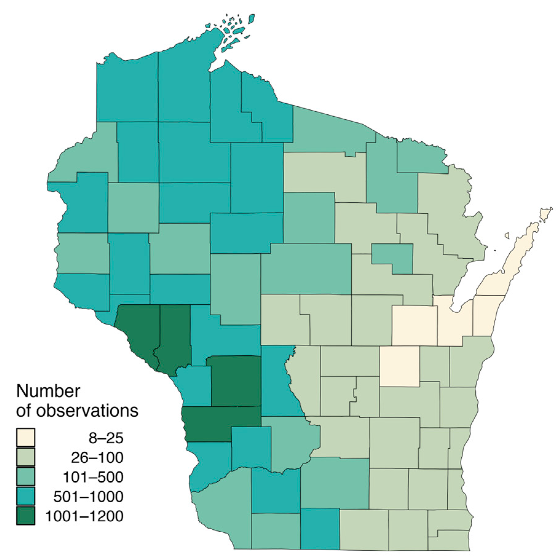
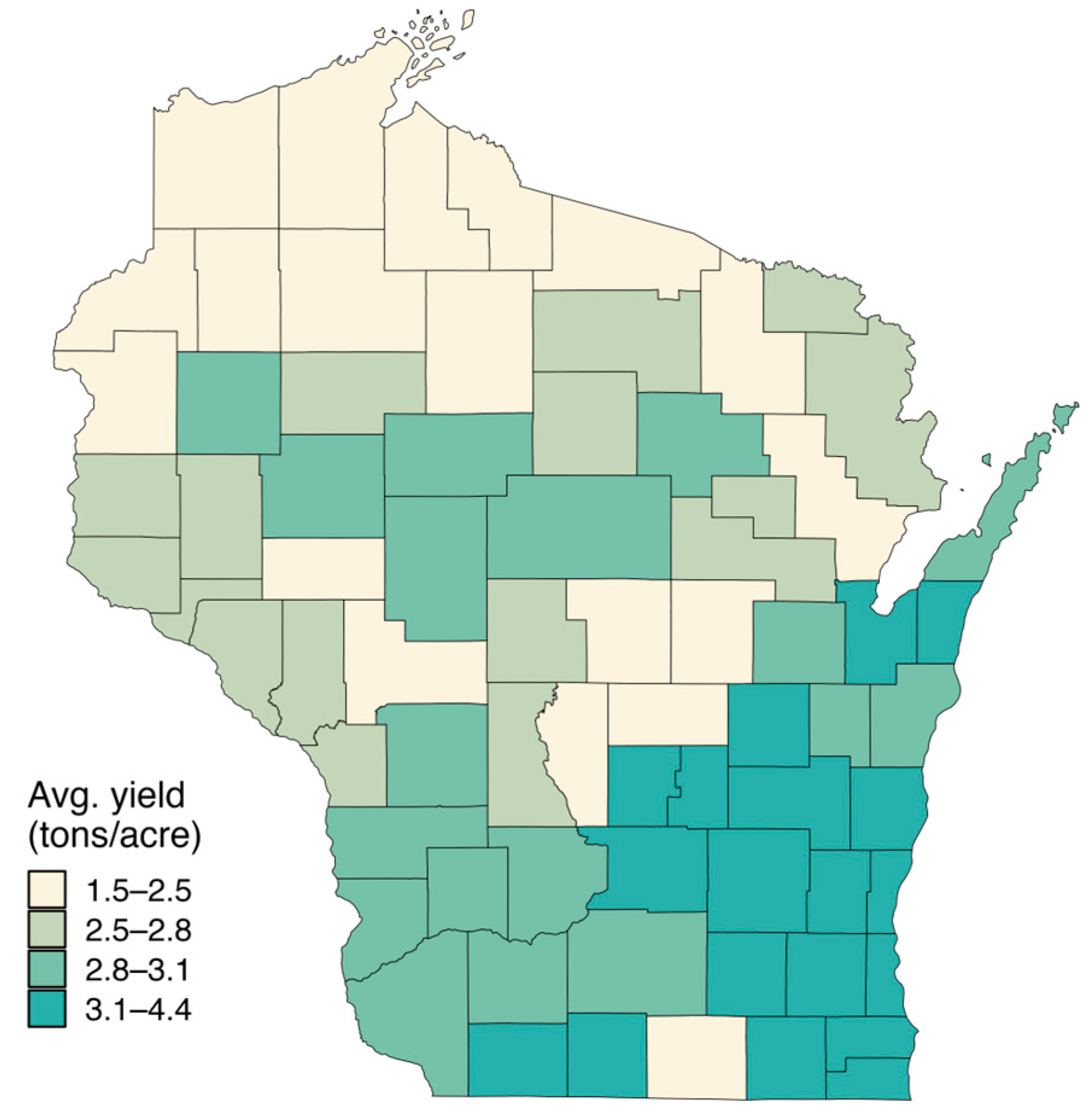
3.1. SSURGO Summary Statistics

The SSURGO database reported 23,889 observations of representative grass yield data with n = 6351 bluegrass–clover, n = 5848 timothy–clover, and n = 11,690 orchardgrass–clover observations. However, there was significant variability in data records across the state of Wisconsin. Brown, Winnebago, Door, Outagamie, and Kewaunee counties had the fewest observations (n = 8, 8, 12, 12, and 22, respectively), while Buffalo, Monroe, Vernon, and Trempealeau counties all had over 1000 observations (n = 1122, 1092, 1072, and 1008, respectively). Notably, the western half of the state, where pastures are more common, had consistently more observations than the eastern half of the state (Figure 1). The average grass yield in Wisconsin was 2.6 ± 1.05 tons/acre (mean ± SD; ~5830 kg/ha), and this varied by region and county (Figure 2). Higher yielding counties tended to be in the southeastern part of the state.

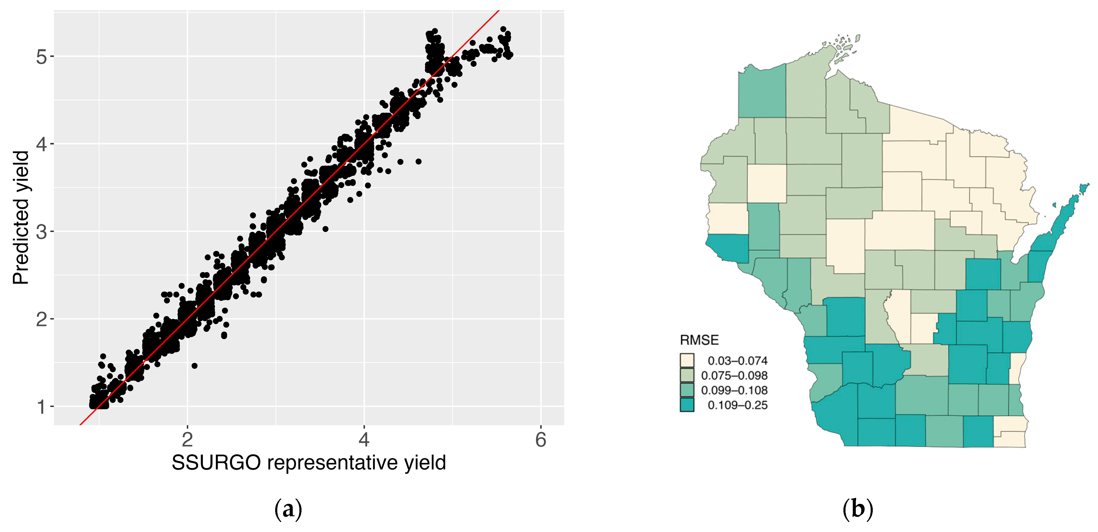
3.2. Random Forest Model Results and Assessment

The final random forest model showed an excellent predictive capability of yield potential as a function of soil properties (Figure 3a, R2 = 0.99, RMSE = 0.11). The average predicted yield was 2.6 ± 1.03 tons/acre (mean ± SD; ~5830 kg/ha). Even though the model fit is heterogenous across Wisconsin counties (Figure 3b) with some areas having better fits than others in the overall model, the average RMSE is still acceptably low (<10% of average yield) and within an excellent range to qualify as a good model fit across the state of Wisconsin. The most important variables influencing the fit of the data in the model were grass species, and soil-associated variation in saturated hydraulic conductivity (Ksat), available water capacity (AWC), and percent slope (Figure 4).

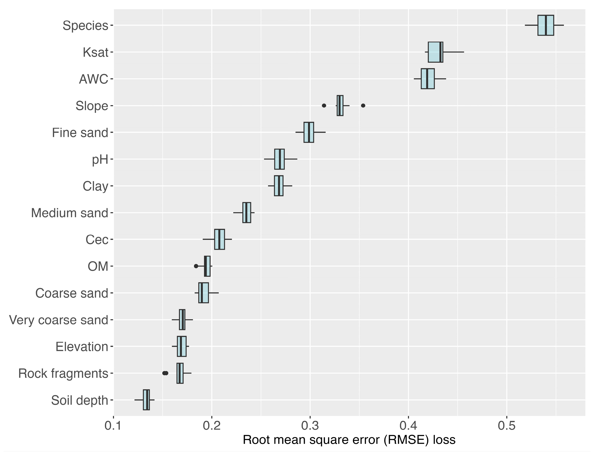
3.3. Effect of Soil Properties on Pasture Yield
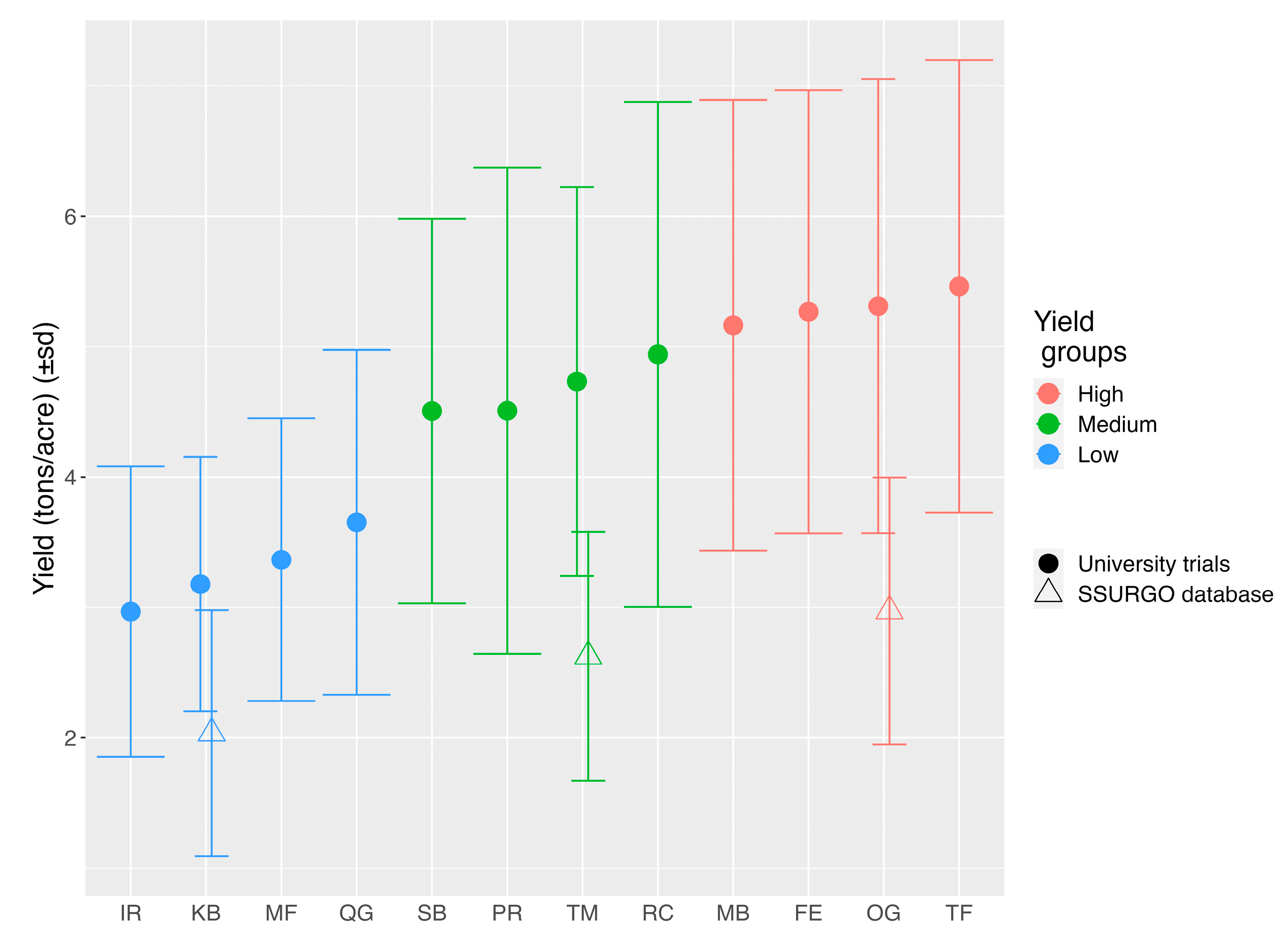
We found opposing impacts of Ksat and AWC such that pasture yield predictions decreased with higher Ksat values (Figure 5b) and increased as AWC decreased (Figure 5c). Ksat, or saturated hydraulic conductivity, is the rate that water moves through saturated soil, and it increases with sand content in the soil. Available water capacity (AWC) is the maximum amount of plant available water that the soil can provide [37]. Because water availability has a direct effect on plant growth [38], it is not a surprise that soil properties related to water retention and movement are important predictors for yield. Pasture yields were also relatively lower on steeper slopes (Figure 5d). Slope also likely affects yield, at least partially, through its impact on water movement or indirectly by impacting soil physical and chemical properties [14]. Steeper slopes are likely contributing to the observation that average yields in the unglaciated Driftless Area in the southwest part of the state is lower than the average yield in the southeast part of the state (Figure 2) where land had been glaciated and has relatively flatter topography.

3.4. Grass Species

Grass species was the most important variable in the random forest model (Figure 4). This suggests that despite the influence of fixed soil characteristics on a farm, producers can still have significant influence on pasture yield by planting higher yielding species. For example, the partial dependence plot (Figure 5a) shows the effect of grass species when all soil properties in the model are held constant. For the purposes of illustration, Figure 6 shows the web application output for a specific soil revealing that yield potential increases by 30% when switching from a low-yielding grass species, such as bluegrass (P. pratensis) to a higher-yielding grass species like orchardgrass (D. glomerata) (Figure 6 and Table 2). Impressively, yield potential increases by ~85% when switching between continuously grazed and rotationally grazed pastures with occupancy < 1 d on a given soil (Figure 6 and Table 2).
SSURGO estimated yields are on average ~40% lower than the yields reported from the UW Extension trials when comparing with species present in both datasets (Figure 7). Differences between the two datasets are not surprising. SSURGO yields are lower than UW Extension trials in part because SSURGO yields are averages from across the entire state including from places with poorer soil conditions than at the research stations used in the plot-level trials. However, the fact that the relationship between species’ yields is consistent in rank order between the two data sources adds confidence to the yield patterns.
We categorized the UW Extension trial species into low-, medium-, and high-yielding groups. Each yield group also contains one species from the soil survey database. The creation of these yield groups allows graziers and grazing planners to obtain a yield estimate for a range of species with similar yields when the model predicts yield for one of the species included in the SSURGO dataset. Having the ability to apply this model to more grass species will increase the utility of the model. The mean yield of the “low-yielding group” is 3.3 tons/acre (range 2.9 to 3.7). This group includes Kentucky bluegrass, Italian ryegrass, quackgrass, and meadow fescue. The mean yield of the “medium-yielding group” is 4.7 tons/acre (range 4.5 to 4.9) and consists of timothy, smooth bromegrass, perennial ryegrass, and reed canarygrass. Lastly, the mean yield of the “high-yielding group” is 5.3 tons/acre (range 5.2 to 5.5) and includes orchardgrass, meadow bromegrass, festulolium, and tall fescue (Figure 7).

3.5. Effect of Grazing Management on Pasture Yield

The Forage Animal Balance Worksheet from NRCS [36] instructs grazing planners to decrease their estimated forage yield by a factor of 0.92 for each day past three days of animal residency in a paddock to arrive at a new forage yield estimation. We supplemented this relationship by reviewing the available literature that compared pasture productivity between continuous and rotationally grazed systems, as well as among rotational grazing management variables (Table 3). A decrease in yield due to increasing rotation length has been documented in several studies. For example, Gurda (2014) compared forage production between mob-grazed (animals rotated on average every 8–24 h) and rotationally grazed (rotated on average every 24–48 h) plots and found nearly a 25% increase in production in the mob-grazed plots. Additionally, Bertelsen et al. (1993) saw an approximately 15% increase in forage availability in a 3 d rotation compared to a 6 d rotation. Lastly, studies document that forage yield in rotational grazing systems is higher than in continuously grazed systems by 50–100% [17,18,19].
We combined the NRCS yield adjustments with the results from our literature review to arrive at the final yield adjustment calculations (Table 3). By integrating the NRCS worksheet with data from the literature, we were able to add information regarding more frequent rotations (less than three days) and compare yield in rotational and continuous grazing operations. These values were used as post hoc adjustments of the pasture yield model to account for user-specified differences in grazing intensity.

3.6. Model Limitations

While the model’s intentional simplicity enhances its usability and transferability, this approach necessarily sacrifices some ability to capture the system’s full complexity that practitioners should be aware of. For example, our model excludes considerations of plant physiology and phenology. Additionally, this model assumes no interaction between soil properties and grazing management on yield potential even though it is reasonable to expect that this could occur given the interactions between grazing, soil physical properties, and pasture production [39]. This could warrant further research to refine pasture yield response estimates. However, the post hoc yield adjustments for rotational occupancy we estimate may be conservative compared to some of the effects of grazing reported in the literature [18,19,21]. By keeping the model simple yet conservative, we have more confidence in the usability of the final model while not overestimating yield outcomes for farmers who may prefer more conservative estimates. For researchers that are interested in implementing these methods in different regions, caution should be used when integrating the post hoc adjustments because it was not developed for regions outside of Wisconsin. It is important to work with local grazing specialists or consult local literature and data records to compare the relationship between yield and grazing intensity. Lastly, soil fertility management may also have an additional effect on yield. However, the SSURGO dataset assumes that nutrients have been managed appropriately in the pastures from which representative yields are reported [30]. The simplicity of this model is both a strength and a weakness.
In addition, the SSURGO representative yield data on which this model is built has certain limitations. For example, because the dataset does not clearly define the management of the pastures from which yield data are collected, the values in the database may come from a range of different pasture systems and management approaches, including differences in timing of harvest, fertility management, pest management, and herd management. Additionally, because SSURGO representative yield data are defined as yield potential for a year in which the weather is close to the 30-year norm [30], it does not account for climate variability (e.g., prediction during critical drought periods) and ongoing changes in climate. Regardless, SSURGO representative yields have been used in other yield models because the large sample size allows analyses across a range of soil types [13,40].

3.7. Pasture Prediction Web-App Tool

To increase the utility of the pasture prediction model for practitioners or grazing planners, we implemented the RF pasture yield model into an R-shiny app (https://connect.doit.wisc.edu/pasturePrediction/) (accessed on 10 February 2025), making it available to use for anyone in the state of Wisconsin. Users simply select their county and the soil type on which to make pasture prediction. Soil types for any place in Wisconsin can be found through the USDA Web Soil Map tool (https://websoilsurvey.nrcs.usda.gov/app/) (accessed on 10 February 2025). Users can manually adjust a few variables specific to their site and then hit “Predict”. Pasture yield predictions are generated across the three grass yield categories and rotational frequencies and are displayed both as a figure (Figure 6) and a table (Table 2). Users can copy the table and paste it into a spreadsheet to save it for further analysis.

4. Conclusions

We created a simple model that predicts pasture yield—a key performance metric for the economic viability of grass-based agricultural systems—across Wisconsin’s wide range of soil and geographic contexts. This model incorporates different grass species and allows adjustments for variation in grazing management. The methods used to create this model are easily replicable with SSURGO datasets from other states in the region. Our analysis of grass yield using the random forest model along with the post hoc multipliers for grazing management suggests that grazing management may be the single largest predictor of grass yield, followed by grass species, and then soil characteristics.
This model is a first step for providing information to farmers that could allow a simple calculation of expected costs and benefits associated with perennial pasture systems and how they vary with different management decisions. A more standardized collection of data from pastures along with information about yearly climate variables (precipitation and temperature), management, and soils will improve future iterations of this model and make it more useful for predicting pasture responses to changing management and climate.

Author Contributions

Conceptualization, E.C., E.B. and C.G.; methodology, E.C.; software, E.C.; validation, E.C.; formal analysis, E.C.; investigation, E.C.; resources, C.G.; data curation, E.C.; writing—original draft preparation, E.C.; writing—review and editing, E.B. and C.G.; visualization, E.C.; supervision, E.B. and C.G.; project administration, E.B. and C.G.; funding acquisition, E.B. and C.G. All authors have read and agreed to the published version of the manuscript.

Funding

This research was funded by the Sustainable Agriculture Systems Coordinated Agricultural Program, Grant No. 2019-68012-29852, from the USDA National Institute of Food and Agriculture.

Data Availability Statement

The analysis code can be found at https://github.com/Grasslands-2/grassGrowth (accessed on 10 February 2025). The original data presented in this study are openly available online at https://websoilsurvey.nrcs.usda.gov/app/ (accessed on 10 February 2025). Extension trial grass yield data are openly available at EDI Data Portal https://doi.org/10.6073/pasta/4f885c86306283ce92e61270946f9c44 (accessed on 10 February 2025).

Acknowledgments

The authors would like to thank Jim Munsch, Laura Paine, and Adam Abel for feedback on model usability; Dan Undersander and Michael Casler for sharing UW Extension data; and Laura Ward Good for help with the interpretation of SSURGO metadata.

Conflicts of Interest

The authors declare no conflicts of interest. The funders had no role in the design of the study; in the collection, analyses, or interpretation of data; in the writing of the manuscript; or in the decision to publish the results.

References

  1. Dartt, B.A. A Comparison of Management-Intensive Grazing and Conventionally Managed Michigan Dairies: Profitability, Economic Efficiencies, Quality of Life, and Management Priorities. Master’s Thesis, Michigan State University, East Lansing, MI, USA, 1998. [Google Scholar]
  2. Kriegl, T. Major Cost Items on Wisconsin Organic, Grazing and Confinement (Average of All Sizes) Dairy Farms. Center for Dairy Profitability, University of Wisconsin—Madison, UWEX. February 2008, p. 6. Available online: https://cias.wisc.edu/directory/tom-kriegl/ (accessed on 10 February 2025).
  3. Undersander, D.; Albert, B.; Cosgrove, D.; Johnson, D.; Peterson, P. Pastures for Profit: A Guide to Rotational Grazing; Cooperative Extension Publications, University of Wisconsin-Extension: Madison, WI, USA, 2014; p. A3529. [Google Scholar]
  4. Winsten, J.R.; Kerchner, C.D.; Richardson, A.; Lichau, A.; Hyman, J.M. Trends in the Northeast Dairy Industry: Large-Scale Modern Confinement Feeding and Management-Intensive Grazing. J. Dairy Sci. 2010, 93, 1759–1769. [Google Scholar] [CrossRef] [PubMed]
  5. Winsten, J.R.; Richardson, A.; Kerchner, C.D.; Lichau, A.; Hyman, J.M. Barriers to the Adoption of Management-Intensive Grazing among Dairy Farmers in the Northeastern United States. Renew. Agric. Food Syst. 2011, 26, 104–113. [Google Scholar] [CrossRef]
  6. Johnson, I.R.; Chapman, D.F.; Snow, V.O.; Eckard, R.J.; Parsons, A.J.; Lambert, M.G.; Cullen, B.R. DairyMod and EcoMod: Biophysical Pasture-Simulation. Aust. J. Exp. Agric. 2008, 48, 621–631. [Google Scholar] [CrossRef]
  7. Baldinger, L.; Vaillant, J.; Zollitsch, W.; Rinne, M. Making a Decision-Support System for Dairy Farmers Usable throughout Europe: The Challenge of Feed Evaluation. Adv. Anim. Biosci. 2015, 6, 3–5. [Google Scholar] [CrossRef]
  8. Hurtado-Uria, C.; Hennessy, D.; Shalloo, L.; Schulte, R.P.O.; Delaby, L.; O’connor, D. Evaluation of Three Grass Growth Models to Predict Grass Growth in Ireland. J. Agric. Sci. 2013, 151, 91–104. [Google Scholar] [CrossRef]
  9. Keating, B.A.; Carberry, P.S.; Hammer, G.L.; Probert, M.E.; Robertson, M.J.; Holzworth, D.; Huth, N.I.; Hargreaves, J.N.G.; Meinke, H.; Hochman, Z.; et al. An Overview of APSIM, a Model Designed for Farming Systems Simulation. Eur. J. Agron. 2003, 18, 267–288. [Google Scholar] [CrossRef]
  10. Cohen, R.D.H.; Stevens, J.P.; Moore, A.D.; Donnelly, J.R. Validating and Using the GrassGro Decision Support Tool for a Mixed Grass/Alfalfa Pasture in Western Canada. Can. J. Anim. Sci. 2003, 83, 171–182. [Google Scholar] [CrossRef]
  11. Jeong, J.H.; Resop, J.P.; Mueller, N.D.; Fleisher, D.H.; Yun, K.; Butler, E.E.; Timlin, D.J.; Shim, K.-M.; Gerber, J.S.; Reddy, V.R.; et al. Random Forests for Global and Regional Crop Yield Predictions. PLoS ONE 2016, 11, e0156571. [Google Scholar] [CrossRef]
  12. Kravchenko, A.N.; Bullock, D.G. Correlation of Corn and Soybean Grain Yield with Topography and Soil Properties. Agron. J. 2000, 92, 75–83. [Google Scholar] [CrossRef]
  13. Lark, T.J.; Spawn, S.A.; Bougie, M.; Gibbs, H.K. Cropland Expansion in the United States Produces Marginal Yields at High Costs to Wildlife. Nat. Commun. 2020, 11, 4295. [Google Scholar] [CrossRef] [PubMed]
  14. Jiang, P.; Thelen, K.D. Effect of Soil and Topographic Properties on Crop Yield in a North-Central Corn–Soybean Cropping System. Agron. J. 2004, 96, 252–258. [Google Scholar] [CrossRef]
  15. Liakos, K.G.; Busato, P.; Moshou, D.; Pearson, S.; Bochtis, D. Machine Learning in Agriculture: A Review. Sensors 2018, 18, 2674. [Google Scholar] [CrossRef] [PubMed]
  16. van Klompenburg, T.; Kassahun, A.; Catal, C. Crop Yield Prediction Using Machine Learning: A Systematic Literature Review. Comput. Electron. Agric. 2020, 177, 105709. [Google Scholar] [CrossRef]
  17. Sollenberger, L.E.; Agouridis, C.T.; Vanzant, E.S.; Franzluebbers, A.J.; Owens, L.B. Prescribed Grazing on Pasturelands. In Conservation Outcomes from Pastureland and Hayland Practices: Assessment, Recommendations, and Knowledge Gaps; Allen Press: Lawrence, KS, USA, 2012; pp. 111–204. [Google Scholar]
  18. Oates, L.G.; Undersander, D.J.; Gratton, C.; Bell, M.M.; Jackson, R.D. Management-Intensive Rotational Grazing Enhances Forage Production and Quality of Subhumid Cool-Season Pastures. Crop Sci. 2011, 51, 892–901. [Google Scholar] [CrossRef]
  19. Paine, L.K.; Undersander, D.; Casler, M.D. Pasture Growth, Production, and Quality under Rotational and Continuous Grazing Management. J. Prod. Agric. 1999, 12, 569–577. [Google Scholar] [CrossRef]
  20. Bertelsen, B.S.; Faulkner, D.B.; Buskirk, D.D.; Castree, J.W. Beef Cattle Performance and Forage Characteristics of Continuous, 6-Paddock, and 11-Paddock Grazing Systems. J. Anim. Sci. 1993, 71, 1381–1389. [Google Scholar] [CrossRef]
  21. Gurda, A. Mob Grazing, from People to Pastures: Weed Biology, Pasture Productivity, and Farmer Perception and Adoption. Master’s Thesis, University of Wisconsin, Madison, WI, USA, 2014. [Google Scholar]
  22. Soil Survey Staff Soil Survey Geographic (SSURGO) Database. Available online: https://sdmdataaccess.sc.egov.usda.gov (accessed on 1 December 2023).
  23. R Core Team. R: A Language and Environment for Statistical Computing; R Foundation for Statistical Computing: Vienna, Austria, 2022. [Google Scholar]
  24. Bocinsky, R. FedData: Functions to Automate Downloading Geospatial Data Available from Several Federated Data Sources; R Package Version 401; 2023. Available online: https://CRAN.R-project.org/package=FedData (accessed on 10 February 2025).
  25. Wickham, H.; Averick, M.; Bryan, J.; Chang, W.; McGowan, L.; François, R.; Grolemund, G.; Hayes, A.; Henry, L.; Hester, J.; et al. Welcome to the Tidyverse. J. Open Source Softw. 2019, 4, 1686. [Google Scholar] [CrossRef]
  26. Kuhn, M.; Wickhan, H. Tidymodels: A Collection of Packages for Modeling and Machine Learning Using Tidyverse Principles; 2020. Available online: https://www.tidymodels.org/ (accessed on 10 February 2025).
  27. Wright, M.N.; Ziegler, A. Ranger: A Fast Implementation of Random Forests for High Dimensional Data in C++ and R. J. Stat. Softw. 2017, 77, 1–17. [Google Scholar] [CrossRef]
  28. Gregorutti, B.; Michel, B.; Saint-Pierre, P. Correlation and Variable Importance in Random Forests. Stat. Comput. 2017, 27, 659–678. [Google Scholar] [CrossRef]
  29. Biecek, P. DALEX: Explainers for Complex Predictive Models in R. J. Mach. Learn. Res. 2018, 19, 5. [Google Scholar]
  30. USDA Soil Survey Geographic (SSURGO) Database. Available online: https://www.fsl.orst.edu/pnwerc/wrb/metadata/soils/ssurgo.pdf (accessed on 1 December 2023).
  31. Jackson, R.B.; Canadell, J.; Ehleringer, J.R.; Mooney, H.A.; Sala, O.E.; Schulze, E.D. A global Analysis of Root Distributions for Terrestrial Biomes. Oecologia 1996, 108, 389–411. [Google Scholar] [CrossRef]
  32. Grömping, U. Variable Importance Assessment in Regression: Linear Regression Versus Random Forest. Am. Stat. 2009, 63, 308–319. [Google Scholar] [CrossRef]
  33. Oldfield, E.E.; Bradford, M.A.; Wood, S.A. Global Meta-Analysis of the Relationship between Soil Organic Matter and Crop Yields. SOIL 2019, 5, 15–32. [Google Scholar] [CrossRef]
  34. Fisher, A.; Rudin, C.; Dominici, F. All Models are Wrong, but Many are Useful: Learning a Variable’s Importance by Studying an Entire Class of Prediction Models Simultaneously. J. Mach. Learn. Res. 2019, 20, 1–81. [Google Scholar]
  35. Undersander, D.; Bertram, M.; Breuer, J.; Cavadini, J.; Crooks, A. Forage Variety Update for Wisconsin; University of Wisconsin—Extension: Madison, WI, USA, 2017; p. A1525. [Google Scholar]
  36. NRCS Forage Animal Balance Worksheet. Available online: https://efotg.sc.egov.usda.gov/#/state/WI/documents/section=3&folder=65188 (accessed on 13 January 2025).
  37. NRCS Soil Quality Indicators. Available online: https://www.nrcs.usda.gov/sites/default/files/2022-10/nrcs142p2_051590.pdf (accessed on 1 June 2023).
  38. Taiz, L. Plant Physiology, 5th ed.; Sinauer Associates: Sunderland, MA, USA, 2010. [Google Scholar]
  39. Greenwood, K.L.; McKenzie, B.M. Grazing Effects on Soil Physical Properties and the Consequences for Pastures: A Review. Aust. J. Exp. Agric. 2001, 41, 1231. [Google Scholar] [CrossRef]
  40. Meehan, T.D.; Gratton, C.; Diehl, E.; Hunt, N.D.; Mooney, D.F.; Ventura, S.J.; Barham, B.L.; Jackson, R.D. Ecosystem-Service Tradeoffs Associated with Switching from Annual to Perennial Energy Crops in Riparian Zones of the US Midwest. PLoS ONE 2013, 8, e80093. [Google Scholar] [CrossRef]
Figure 1. Number of grass yield observations from SSURGO database used in model fitting in Wisconsin counties.
Agronomy 15 00437 g001
Figure 2. Average grassland yield (tons/ac) by county in the SSURGO database.
Agronomy 15 00437 g002
Figure 3. Final model fit of random forest model using soil SSURGO data to predict pasture yield. (a) Predicted yield from final fitted model (Y-axis) compared to observed SSURGO representative yield (X-axis). Red line represents a 1:1 relationship between the two. RMSE = 0.11, R2 = 0.99. (b) Map of root mean square error (RMSE) of grass yield model across Wisconsin showing the range of model fits by county.
Agronomy 15 00437 g003
Figure 4. Permutation-based variable importance plot. Values are the change in RMSE after 1000 permutations in which the model is run with a resampled value from the empirical distribution of each variable. Larger values reflect more important variables.
Agronomy 15 00437 g004
Figure 5. Partial dependance plots of the 4 most important variables in the random forest model: (a) grass species, (b) soil-associated variation in saturated hydraulic conductivity (ksat), (c) available water capacity (AWC), and (d) percent slope. Gray lines represent individual yield predictions for a soil in which all parameters are held constant except the parameter on the x-axis. Black dotted line represents the average predicted yield across the range of the variable.
Agronomy 15 00437 g005
Figure 6. Demonstration of yield potential of a single soil across grazing management and grass species, as displayed in the R-shiny web application figure.
Agronomy 15 00437 g006
Figure 7. Average yield for grass species from University of Wisconsin Extension variety trials, 1983–2017 (circles), and soil survey yield averages (triangles), along with resulting yield groupings (blue = low-yielding, green = medium-yielding, and red = high-yielding species). Species abbreviations: IR = Italian ryegrass; KB = Kentucky bluegrass; MF = meadow fescue; QG = quackgrass; SB = smooth bromegrass; PR = perennial ryegrass; TM = timothy grass; RC = reed canarygrass; MB = meadow bromegrass; FE = festulolium; OG = orchardgrass; TF = tall fescue.
Agronomy 15 00437 g007
Table 1. Soil properties included in feature selection for predicting grass yield. Soil properties were excluded when the data available for the property had >50% missing values in the dataset (NA), near zero variance, or if they were very highly correlated (r > 0.90) with other properties. Properties were included in the model if the literature showed that they were important predictors, or if initial exploration showed a visual relationship between the soil variable and grass yield. Soil properties were accessed from USDA Soil Survey.
Soil PropertyCitationFinal Model?
Available water capacity (AWC) Yes
Cation exchange capacity (CEC) Yes
Clay (%)[14]Yes
Coarse sand (%)[14]Yes
Coarse silt (%) No—Too many NAs
Depth to bedrock Yes
Electrical conductivity No—No variance
Elevation[12]Yes
Fine sand (%)[14]Yes
Fine silt (%) No—Too many NAs
Medium sand (%) Yes
Organic matter (%)[33]Yes
pH[14]Yes
Particle density No—Too many NAs
Rock fragments (3–10 in) Yes
Rock fragments (>10 in) No—No variance
Sand (%)[14]No—Highly correlated
Saturated hydraulic conductivity (Ksat) Yes
Silt (%) No—Highly correlated
Slope[12,14]Yes
Very coarse sand Yes
Table 2. Yield potential of a single soil across grazing management and grass species, as displayed in the R-shiny web application chart.
Occupancy (Days)Low-Yielding SpeciesMedium-Yielding SpeciesHigh-Yielding Species
Yield (Tons/Acre)
Continuous1.491.841.95
71.722.122.25
32.172.692.84
12.292.832.99
<12.743.393.59
Table 3. Post hoc yield adjustment factor to yield potential as predicted from random forest model of soil properties.
Rotation Frequency (Days)NRCS Yield AdjustmentFinal Yield Adjustment 1
<1NA1.2 2
1NA1.0 2
2NA1.0 3
3NA0.95 3
40.920.92 3
50.850.85 3,4
60.780.78 3
70.720.72 3
ContinuousNA0.65 5
1 See references used to derive the final yield adjustment: 2 [21], 3 [36], 4 [20], and 5 [17,18,19].
Disclaimer/Publisher’s Note: The statements, opinions and data contained in all publications are solely those of the individual author(s) and contributor(s) and not of MDPI and/or the editor(s). MDPI and/or the editor(s) disclaim responsibility for any injury to people or property resulting from any ideas, methods, instructions or products referred to in the content.

