Article

A Canopy Height Model Derived from Unmanned Aerial System Imagery Provides Late-Season Weed Detection and Explains Variation in Crop Yield

1
Department of Crop and Soil Sciences, North Carolina State University, Raleigh, NC 27695-7620, USA
2
N.C. Plant Sciences Initiative, 840 Oval Drive, Campus Box 7825, Raleigh, NC 27695-7601, USA
*
Author to whom correspondence should be addressed.
Agronomy 2025, 15(12), 2885; https://doi.org/10.3390/agronomy15122885
Submission received: 4 November 2025 / Revised: 3 December 2025 / Accepted: 5 December 2025 / Published: 16 December 2025
(This article belongs to the Section Weed Science and Weed Management)

Abstract

Weeds pose a ubiquitous challenge to researchers as a source of unintended variation on crop yield and other metrics in designed experiments, creating a need for practical and spatially comprehensive techniques for weed detection. To that end, imagery acquired using unmanned aerial systems (UASs) and classified using pixel-based, object-based, or neural network-based approaches provides researchers a promising avenue. However, in scenarios where spectral differences cannot be used to distinguish between crop and weed foliage, where physical overlap between crop and weed foliage obstructs object-based detection, or where large datasets are not available to train neural networks, alternative methods may be required. For instances where there is a consistent difference in height between crop and weed plants, a mask can be applied to a canopy height model (CHM) such that pixels are determined to be weed or non-weed based on height alone. The CHM Mask (CHMM) approach, which produces a measure of weed area coverage using UAS-acquired, red–green–blue imagery, was used to detect Palmer amaranth in Sweetpotato with an overall accuracy of 86% as well as explain significant variation in sweetpotato yield (p < 0.01). The CHMM approach contributes to the diverse methodologies needed to conduct weed detection in different agricultural settings.

1. Introduction

Weeds play a pivotal role in agroecosystems, prompting nationwide, institutional-scale research to mitigate their negative effects [1]. In the context of agricultural research, weeds are ideally controlled for or excluded altogether to prevent their confounding effects on yield [2], soil nutrients [3], and other endpoints. While modern agriculture has many tools available for this purpose, there are scenarios in which weeds may be difficult to control. Herbicide resistance is a well-known phenomenon in conventionally managed systems [4]. A research objective may call for herbicide applications to be withheld or reduced, which can incur weed growth [5,6]. In studies involving organic management, hand-weeding may be required [7,8], but hand-weeding is labor-intensive and often impractical at the field scale. In scenarios where weeds cannot be adequately controlled, methods for characterizing weeds are essential to account for their growth and influence.
Weediness has been traditionally characterized by measuring weed biomass and density. However, these approaches are time-consuming, and samplings may not capture the spatial and temporal heterogeneity characteristic of weed populations. Additionally, if weeds need to be measured at points late in the growing season, weed patches comprised of densely packed, large plants may obstruct accurate counts and biomass measurements.
Unmanned aerial system (UAS)-based approaches offer a means of characterizing weed pressure in agricultural systems when time and labor resources are not available to measure weed biomass and density [9]. Utilizing UAS imagery in this way depends on image analysis techniques that allow for weeds to be distinguished from crops (i.e., weed detection). Multispectral (MS) sensors have been shown to be more effective than red–green–blue (RGB) cameras for resolving the spectral reflectance of crops and weeds [10], although MS sensors are more costly and require more user expertise. Classification approaches have ranged from the built-in pixel-based and object-based approaches available in Geographical Information System (GIS) applications (e.g., ArcGIS) to custom-developed object-based image analysis algorithms [11]. While object-based classification may offer a solution for weed detection when crop and weed plants cannot be resolved by spectral differences alone, object-based detection is hampered by physical overlap between crop and weed plants [12,13]. Neural networks have been used effectively for weed detection, but with the drawback of requiring large training datasets [14,15]. The respective limitations of conventional classification approaches can be overcome by alternative methodologies tailored for specific scenarios.
A canopy height model (CHM), which is derived from the digital surface model (DSM) generated when mosaicking UAS imagery, offers a viable means for characterizing and mapping late-season weed pressure using plant height alone. Where there is a consistent height difference between crop and weed plants, such as a low-lying cash crop and a weed community comprised predominantly of tall-growing species, the CHM could hypothetically be leveraged for weed detection. Studies have used CHMs for weed detection by integrating them with spectral and other types of information [16,17]. However, there are few studies demonstrating the potential of the CHM used alone to detect weeds and explain variation in cash crop yield.
An approach for using the CHM for late-season weed detection was developed in the course of a field study investigating the potential for management practices to influence soil health during organic transition. In year 3 of the study, when Sweetpotato (Ipomoea batatas) (SP) was planted, a flush of Palmer amaranth (Amaranthus palmeri S. Wats.) (PA) was observed to emerge 43 days after planting, in late July. PA is a tall-growing weed and can cause major yield losses in SP [18]. Various approaches were used for weed detection, including pixel-based classification, object-based classification, neural networks, and plant height differences via the CHM. The objective of this study was to develop an effective means of weed detection based on CHM anomalies within the constraints posed by the available data, which entailed a limited dataset (single flight) of RGB imagery exhibiting dense crop and weed foliage with a high degree of spectral and physical overlap.

2. Materials and Methods

2.1. Experimental Background

An experiment to evaluate the impact of management practices on soil health during organic transition took place at the Upper Coastal Plain Research Station near Rocky Mount, NC (35.89 N, 77.68 W) in the years 2020 to 2023. The treatments included additions of carbonaceous soil amendments (compost, biochar, or a mixture of the two) and cover cropping implemented in a factorial, randomized complete block design. Plots were 9.1 by 4.9 m in size (44.6 m2), and the entire study area was 0.53 ha in size. For additional details concerning the site and experimental design, see Teasley et al. [19].
Single-species cover crops were planted in the fall of each year prior to the cash crop and terminated in spring by disking. This report will focus on year 3 of the study, where crimson clover (Trifolium incarnatum L.) preceded SP. In NC, SP culture typically involves planting in raised beds approximately 2 dm tall. SP was planted on 15 June 2023. On 4 October, SP roots were dug up with a two-row chain digger (Yield Max Gen. 2 Short Bed Digger, Strickland Brothers Enterprises, Inc., Spring Hope, NC, USA) and roots within a sampled area (372 dm2), chosen based on visual assessment of whole-plot representation, were weighed to quantify yield. Yield was reported as the fresh weight of total marketable yield, or the sum of jumbo, “no.1”, and “no.2” grades [20].

2.2. UAS Parameters

Aerial imagery was collected using a Mavic 2 Pro (DJI, Shenzhen, China) UAS equipped with a 20-megapixel, RGB camera to monitor crop growth. Ground control points with known coordinates were established at the four corners of the field using an Emlid Reach RS2+ real-time kinematic (RTK)-GNSS system (Emlid Tech KFT, Budapest, Hungary). Flights were conducted at an altitude of 30 m and at a time close to solar noon (11:00–13:00) under clear sky conditions. Imagery was collected by flying a serpentine pattern over the field using a third-party flight planning application (Drone Deploy, San Francisco, CA, USA), which ensured that imagery was collected with 80% front overlap and 75% side overlap.
With a field size of 0.53 ha and a flight altitude of 30 m, it required 155 images to capture the field along with substantial margins (~10 m) to ensure complete capture of the study area. The orthomosaic and DSM were generated using Metashape v. 2.0.1 (Agisoft, St. Petersburg, Russia). The DSM is generated from a dense point cloud created during the mosaicking process, which captures surface structures and vegetation by applying the Structure from Motion technique. After orthorectification using ground control points, residual errors for ground control points were less than 0.1 m. The resulting spatial resolution or ground sample distances for the orthomosaic and DSM were 0.71 and 2.8 cm pixel−1, respectively. All ensuing analyses were carried out using ArcGIS Pro v. 3.4.2 (ESRI, The Redlands, CA, USA).

2.3. Visual Assessments of Weediness

The fields were relatively weed-free until 28 July, 43 days after planting, when PA was observed to have recently emerged at varying densities across plots. From the point of emergence in late July, PA grew rapidly, with some plants taller than 150 cm by 1 September. On 1 September, visual assessments of weediness were conducted by one person, and plots were assigned a rating on a scale from 1 to 5, with 5 being the weediest. Photos of plots across a range of weediness ratings can be viewed in Figure S1.

2.4. Aerial Image Collection and Analysis

The rationale for collecting UAS imagery immediately after conducting the visual weediness assessment was to have quantitative data by which to corroborate the results of the subjective visual assessment. It was initially hoped that conventional image classification approaches (i.e., pixel-based, object-based, or neural networks) would provide a viable means to resolve PA and SP and obtain a coverage area for each class within plots, thereby providing an objective metric of weed pressure.
For pixel- and object-based classification, training samples of SP, PA, soil, and shadow were created from four 4 m2 quadrats at positions chosen semi-randomly on the orthomosaic to ensure the presence of all four classes. For object-based classification, segmentation was applied using the built-in feature in ArcGIS Pro. A maximum likelihood classifier was used for pixel- and object-based approaches. Neural networks were implemented using ArcGIS Pro’s built-in deep learning feature. A variety of neural networks (i.e., Res2Net, SingleShotDetector, FasterRCNN, YOLOv3, and RetinaNet) were trained using 100 manually labeled weed patches identified in the orthomosaic.

2.4.1. CHM Mask Approach

The use of a CHM for weed detection is based on distinguishing tall weeds from a low-lying cash crop based on plant height alone. The potential for this approach was realized upon inspection of the DSM, where PA growth was evident (Figure 1a). By applying a mask to the CHM at a chosen height, pixels corresponding to taller objects in the field can be distinguished as weeds. In this way, the “CHM Mask” (CHMM) approach provides a means of characterizing weed pressure within plots. The output is a measure of “weed” area, or the total area of pixels above the chosen mask height.
To produce a CHM, both a DSM and a digital terrain model (DTM) are required. The DSM is produced from the point cloud generated from UAS imagery collected during crop growth and captures the structural features of growing plants in the field. A DTM needs to only represent the bare earth surface, and can be acquired from UAS imagery collected prior to crop planting [21]. The CHM is created by subtracting the DTM from the DSM, and pixel values in the resulting CHM are plant heights relative to the soil surface.
Generating the CHM in this way has important implications for the CHMM. Subtracting the DTM from the DSM removes the variation in topography and ensures that pixels are representative of plant heights. If tall weeds are to be distinguished from a low-lying cash crop by height alone, any variation in the topography of the field not captured by the DTM will cause biases in weed detection. For example, SP foliage growing in higher areas on the field (e.g., bed ridges) can be misclassified as weeds. Conversely, weeds growing in the relatively low areas of the field (e.g., bed troughs) can be misclassified as non-weeds. The DTM used in this study was generated from UAS imagery collected in February, at a point of minimal cover crop growth and before SP beds were formed (Figure 1b). This allowed for field-scale variation in topography to be addressed (Figure 1c), but it did not address topographical variation due to SP beds.
After CHM creation, a mask height must be chosen. This should be done judiciously, as a mask height that is too high will result in less sensitive detection for shorter weeds and weeds growing in the troughs between SP beds. Also, a higher mask height increases the number of zero observations (i.e., plots with no weed area), which is not ideal for statistical analysis (Section 2.5.2). Conversely, a lower mask height can cause increased interference from SP foliage on bed ridges being misclassified as weed. In the approach described here, mask height determination initially involved a qualitative assessment to determine an appropriate height range, followed by a quantitative evaluation of mask heights in that range.

2.4.2. Qualitative Determination of Mask Height Range

In ArcGIS, a copy of the CHM layer was generated as a CHMM layer and was set to have a 2-class symbology, where pixels below a given height were considered “non-weed” and pixels above that height as “weed” (Figure 1d). The weed class was set to have a prominent symbology (e.g., color red), and the interval adjustment tool under the histogram tab was used to adjust the mask height. With each adjustment, the CHMM layer was qualitatively assessed for adequate capture of PA-infested areas by comparing it with the orthomosaic. Using this approach, it was possible to visualize when the mask height was set too low, capturing the ridges of SP beds, or too high, with an increasing number of plots having no “weed” area. After determining a suitable range of mask height values, four CHMM layers were generated using differing mask height values within that range for further quantitative assessment.

2.4.3. Quantitative Evaluation of Mask Heights

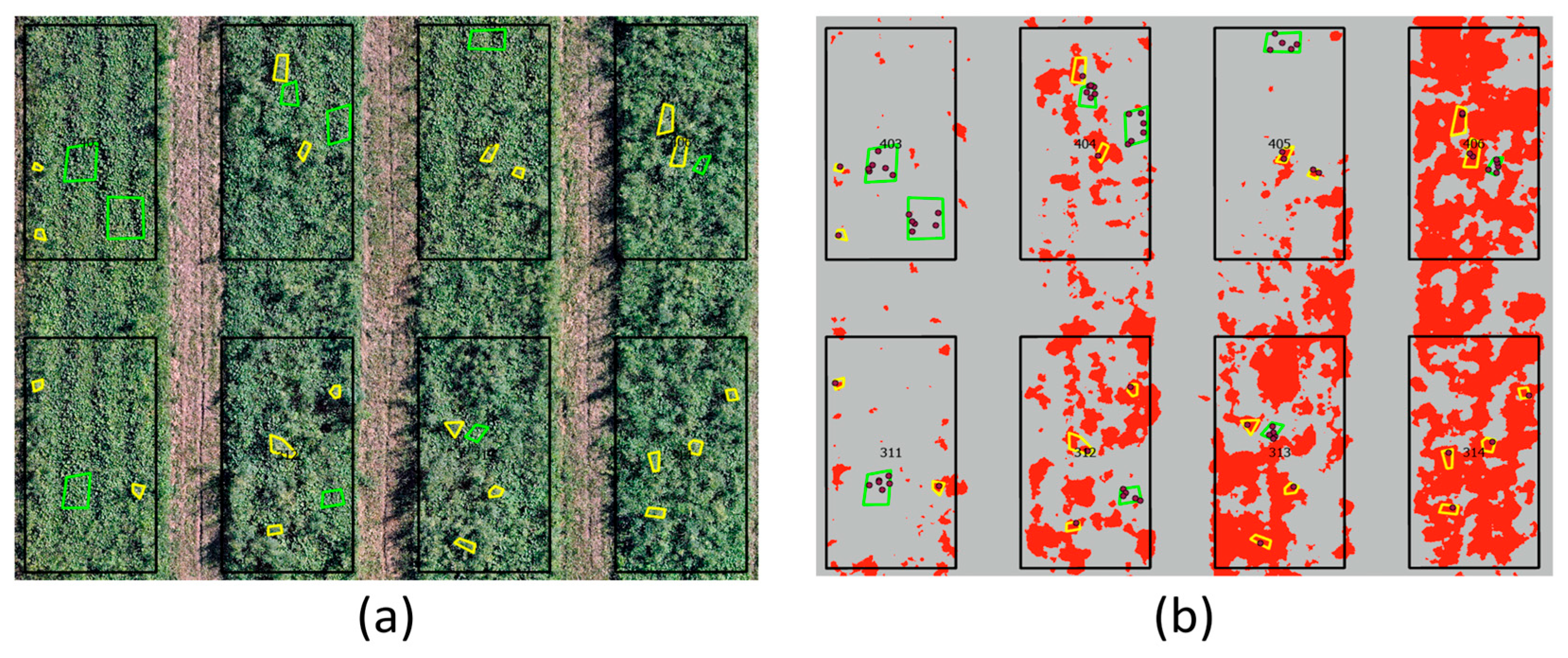
To quantitatively assess different mask heights, CHMM layers generated using different mask heights were evaluated using the accuracy assessment feature in ArcGIS Pro. Accuracy assessment samples were created by generating a polygon layer delineating weed and non-weed areas, which were visually identified using the orthomosaic (Figure 2a). Non-weed areas were sampled to span the ridge and trough of an SP bed. Inclusion of the ridge is important, as SP foliage here has a higher risk of being classified as a false negative for the weed class (i.e., a true “negative” with respect to the weed class, falsely classified as weed). For weed samples, polygons were traced around randomly selected PA plants. At least one weed and non-weed sample was obtained from each plot, except in cases where plots had no weeds. Generally, two or three weed samples were selected from each plot to have a more consistent spatial representation of both classes. The resulting layer of accuracy assessment samples contained 70 non-weed and 116 weed samples, with cumulative areas of 63.8 m3 and 22.7 m3, respectively.
The accuracy assessment feature was then used to generate 500 points within the sample polygons using stratified random sampling, which resulted in at least one assessment point being allocated to each sample (Figure 2b). Then, the accuracy assessment was carried out, comparing the class values of the CHMM to the class values of the assessment points. This procedure was repeated for the four CHMM layers generated from each mask height, and confusion matrices were generated for each layer. In addition to the overall accuracy, which indicates the number of correct classifications across all classes, the confusion matrix shows results for user accuracy, producer accuracy, and Cohen’s kappa statistic. The user and producer accuracies reflect the rate of false positives or false negatives for a given class, respectively.

2.5. Statistical Analysis

Analysis of variance (ANOVA) was carried out using SAS version 9.4 (SAS Institute, Cary, NC, USA) using the GLIMMIX procedure, with block (replicate) set as a random effect. The experimental treatments, amendment type and cover crop, were used as predictors for SP yield, weediness (visual rating), and CHMM weed area. In cases where overall effects in the model were significant, post hoc testing was conducted using Tukey’s HSD correction for multiple comparisons when there were more than two levels to compare. Weediness metrics were also used as predictors for SP yield. The visual rating was treated as a categorical predictor so as not to assume equal spacing between ratings. To obtain parameter estimates and a slope for the CHMM weed area, the SOLUTION option was passed. Diagnostic plots for all models were verified to adhere to assumptions of homoscedasticity and normality.
The weediness metrics, which include the visual rating and CHMM weed area, were originally acquired with the intention of using them as covariates for explaining variation in cash crop (SP) yield, assuming that weediness was unrelated to the treatments. Prior to including either of the weediness metrics as a covariate, the cover crop treatment was found to be significant (p < 0.01) as a predictor for yield. However, including either weediness metric as a covariate rendered the cover crop term insignificant, suggesting that the weediness metrics explain similar variation in yield as the cover crop treatment. A Pearson’s Chi-square test of independence revealed a strong association (p < 0.0001) between the visual rating and the cover crop factor, further suggesting a relationship between weediness and cover cropping. Therefore, the weediness metrics were modeled as response variables (Section 2.5.1 and Section 2.5.2) to assess for relationships with the treatments, and the cover crop term was excluded from models where a weediness metric was included as a predictor based on those findings.
It was generally observed that block, when set as a random effect, returned covariance estimates that were close to zero and small in comparison to the residual error. Since a coefficient of determination (r2) is an inappropriate metric for mixed-effects models [22], the decision was made to gain further insight into the relationship between CHMM weed area and SP yield using simple linear regression. The amendment type term was able to be excluded from the model by removing observations corresponding to an unfertilized control, which was the source of significant differences attributable to that treatment.

2.5.1. Visual Rating of Weed Pressure as a Response Variable

The visual rating of weediness was modeled as a multinomial, ordinal response variable. PROC GLIMMIX was used with a multinomial distribution and a cumulative logit link function. In cases where main effects were significant (p < 0.05), odds ratios were determined to make inferences as to the relationship between the experimental treatments, amendment type and cover crop, and the visual rating. Pair-wise comparisons of treatment levels were considered significant if the 95% confidence interval did not include one, which would otherwise indicate equal odds of receiving the same rating between levels.

2.5.2. Modeling CHMM Weed Area as a Response Variable

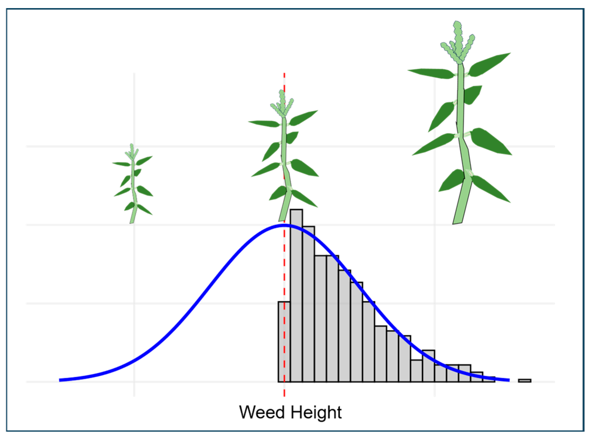
The distribution of CHMM weed area exhibited strong over-dispersion, where variance (928,000 dm2) was high relative to the mean (840 dm2), and a right-skewed distribution (Figure 3). This was not surprising, as the CHMM only detects weed plants taller than the mask height and subsequently has a distribution that is inherently left-censored (Figure 4). The most suitable option for modeling the CHMM weed area as a response was found to be the gamma distribution, which can accommodate over-dispersed and skewed response variables. While the gamma distribution does not allow for the inclusion of zero, this was circumvented by modeling y + 1, the implication of which is the assumption of at least 1 dm2 of weed coverage in each plot, which is reasonable given field observations and is a negligible area in comparison to the plot area (4460 dm2). A log link function was used, and the optimization method was set to adaptive quadrature at the recommendation of SAS staff [23]. This approach produced residual plots that exhibited adherence with the assumptions of ANOVA (Figure S2). Example code for implementing the gamma distribution in PROC GLIMMIX can be viewed in Supplementary Information.

3. Results and Discussion

3.1. Initial Classification Attempts

Pixel-based, object-based, and deep learning approaches could not effectively distinguish between SP and PA foliage. It was clear from visual inspection that the pixel-based classifier could not effectively distinguish between PA and SP due to their similar spectral reflectance (Figure S3a,b). Object-based classification using ArcGIS’ segmentation feature was also not effective, as the generalization provided by segmentation did not provide an effective means of capturing the contrasting leaf architecture between SP and PA (Figure S3c,d). This problem was exacerbated by the high degree of physical overlap between the species.
ArcGIS’ deep learning tools were not sufficient as a classification approach. A variety of neural networks (e.g., Res2Net, SingleShotDetector, FasterRCNN, YOLOv3, and RetinaNet) intended for object detection were trained using 100 labels of weedy patches that were visually identified in the orthomosaic. Among all trained models, the SingleShotDetector achieved the highest precision score of 0.41, indicating that only 41% of weed labels in the validation set were correctly identified. This was deemed as insufficient precision for the intended purpose of weed detection.

3.2. Choosing the Optimum CHM Mask Height

Based on the initial, qualitative assessment of the mask height as described in Section 2.4.2, it was estimated that the optimal mask height would be between 4.3 and 5.5 dm above the DEM. Visual examination of the CHMM layer produced using a mask height of 4.3 dm showed what appeared to be interference from the ridges of SP beds, while the CHMM of the 5.5 dm mask height showed a larger number of plots with no pixels above the mask height. Four CHMM layers were produced using mask heights within the estimated range, and all were assessed using the accuracy assessment described in Section 2.4.3.
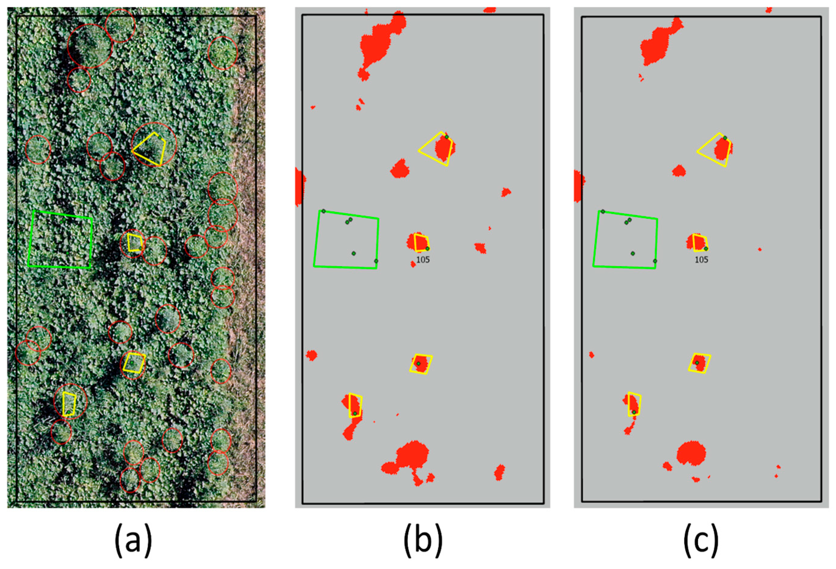
The results from confusion matrices for the range of mask heights tested are shown in Table 1. Overall accuracy and Kappa values were highest and similar for the mask heights of 5.1 and 5.5 dm. However, the 5.1 dm mask height was the most successful at balancing false positives and false negatives, as is evident from the user and producer accuracies for the weed class, respectively. Visual inspection of the classified raster showed that increasing the mask height from 5.1 dm to 5.5 dm shrank the areas classified as weeds (Figure 5), causing more accuracy assessment points designated as weeds (i.e., true weeds or “positives” for the weed class) to be classified as non-weeds and increasing the false positive error rate for the weed class. Accordingly, the user accuracy of the weed class decreased from 72% to 62% while the user accuracy for the non-weed class increased from 91% to 97%, indicating that fewer non-weeds (SP foliage) were classified as weeds (PA). The higher user accuracy for the weed class, achieved at the expense of lower non-weed class user accuracy, was deemed a suitable trade-off, as the weed class was of primary interest, and the user accuracy of the non-weed class was still high (>90%).
Decreasing the mask height from 5.5 dm to 5.1 dm simultaneously decreased the producer accuracy for the weed class from 88% to 75%, which is to say that the false negative rate (i.e., number of non-weed samples classified as weed) increased. While a lower producer accuracy is not desirable in and of itself, the 5.1 dm mask height achieved the best balance between false positives and false negatives while maintaining good overall accuracy (86%), making it the optimal choice of mask height. All discussion henceforth will be regarding the results of the CHMM using the 5.1 dm mask height.

3.3. Cash Crop Yield

The cover crop treatment was a significant predictor of SP yield (p < 0.01),where cover cropping decreased SP yield relative to winter fallow. The least-square means of total marketable yield for the cover-cropped and winter-fallow treatments were 42.9 and 36.5 Mg·ha−1, respectively. The amendment type treatment was also significant (p < 0.05), with the unfertilized control having the lowest yield, which was significantly different from the compost and biochar groups (Table S1). The interaction between the amendment type and cover crop treatments was not significant (p > 0.05).
The reason that the preceding leguminous cover crop decreased SP yield is discussed at length in Teasley et al. [19]. The cover cropped treatment exhibited increased weediness (Section 3.4.2). Enhanced weed growth in the cover cropped treatment likely resulted from late-season N mineralization that was caused by late termination in mid-May, a high cover crop residue C:N ratio of 32, and substantial N input through cover crop biomass (91 kg·N·ha−1). Increased weed pressure has been previously observed to result from increased soil inorganic N resulting from a preceding leguminous cover crop [3,5,24,25].

3.4. Weediness Metrics

3.4.1. Comparison of the Visual Rating and CHMM

In a model with the visual rating as a predictor for CHMM weed area, the least-square means of CHMM weed area increased with rating (Table 2). Visual estimates of weed cover were previously shown to be well correlated to actual weed cover as well as weed biomass [26]. The observed agreement between the visual rating and CHMM weed area is not surprising, as both approaches are sensitive to the tallest and most visually striking part of weed patches. The finding of significant correlation with the visual rating shows that the CHMM weed area provides an effective quantitative metric by which the subjective visual assessment can be corroborated. While the subjective assessment was found to be more sensitive to yield variation (Section 3.4.3), it is prudent to question a subjective assessment unvalidated by a quantitative approach. This makes the visual assessment and the CHMM approach a powerful combination for situations where weediness needs to be characterized efficiently and at low cost, such as large agronomic trials.

3.4.2. Weediness Metrics Used as Response Variables

Both the visual rating and CHMM were included in separate models as the response variable to determine relationships with the experimental treatments and compare model results. In both models, the cover crop treatment was a strong predictor of weediness (p < 0.0001). In the ordinal regression model for the visual rating, cover-cropped plots had 12.3 times higher odds (95% confidence interval: 3.62–41.9) of receiving a higher weediness rating than winter fallow plots. The least-square means of CHMM weed area for cover-cropped and winter-fallow plots were 1002 and 156 dm2, respectively. These results demonstrate a strong, positive relationship between cover cropping and weediness, providing further evidence of the redundancy between the cover crop treatment and weediness metrics first discussed in Section 2.5 and justification for removing the cover crop term as a predictor when including a weediness metric for modeling SP yield.

3.4.3. Weediness Metrics as Predictors for Crop Yield

The weediness metrics, namely the CHMM weed area and the visual rating, were significant predictors for SP yield (p < 0.01). For the visual rating, plots receiving the highest ratings of 4 and 5 exhibited yield losses (Table 2). The plots that received a score of 1 (least weedy) had a numerically intermediate yield, suggesting that conditions promoting weed growth (e.g., elevated soil inorganic N) also promote crop growth to some extent. For example, weed growth and yield were simultaneously low in the unfertilized control (Table S1).
Table 2. SP yield as predicted by the visual rating and CHMM weed area. The CHMM weed areas in column three are least-square mean equivalents for the visual ratings as determined by using the visual rating as a predictor for CHMM weed area. Letters denote Tukey-adjusted significant differences within the same column.
Visual Rating of WeedinessSP Root Yield
(Mg·ha−1)
(via Weed Rating) 1
CHMM Weed Area (dm2) 2SP Root Yield (Mg·ha−1)
(via CHMM) 3
143.3 abc82.9 c48.1 (±1.62) 4
247.5 ab265 bc47.5 (±1.49)
350.7 a572 ab46.3 (±1.34)
438.6 bc1380 a43.3 (±1.54)
533.0 c2000 a41.0 (±2.11)
1 The predicted yields in column two were determined from a model with the visual weediness rating and amendment type as predictors for SP yield. 2 The CHMM weed area values in column three are the least-square means of weed area for each weediness rating as determined using a model with amendment type and the visual weediness rating as predictors for CHMM Weed Area. 3 The yields in column four were predicted using the CHMM weed area equivalents for the visual rating in column three in a model with amendment type and CHMM weed area as predictors for yield. 4 Values in parentheses are the standard errors of the predicted yields.
In the model where SP yield was predicted by CHMM weed area, weed area was significant (p < 0.01) and had a slope of −0.0037, meaning that for every additional 1000 dm2 of weed area, SP yield decreased by 3.7 Mg·ha−1. This magnitude of yield loss was lower than what was exhibited by the visual weediness rating (Table 2), which appeared to exhibit a quadratic trend, with SP yield at the lowest and highest weed ratings lower than the yield at intermediate weed ratings. However, when the quadratic term was tested for the continuous CHMM predictor, it was found to be insignificant (p > 0.05). This is likely due to the insensitivity of the CHMM approach to short weeds (i.e., below the mask height) and consequent inability to distinguish between varying conditions of lesser weed pressure. When simple linear regression was used, a similar slope (−0.0050, p < 0.001) was obtained to that of the mixed-effect model, and the r2 value was 0.25, indicating substantial unexplained variation (Figure 6).
Unexplained variation in SP yield may be implicated with the ability of the CHMM to integrate whole-plot weediness. Since yield is determined from a relatively small area sampled within plots, and the distribution of weeds tends to be patchy, better correlation may have resulted from constraining the CHMM area only to the areas where yield was sampled. Many plots were observed to have high weed pressure at the edges, whereas the central part of the plots was less infested. Since the area sampled for yield determination tended to be chosen in a central location of the plot, plots with high weed pressure at the edges might still have relatively good yields. While it would be impractical to constrain the CHMM to the exact areas where SP root samples were collected, which varied based on areas visually assessed to provide whole-plot representation, the issue posed by weed-infested plot edges could be mitigated simply by excluding plot margins from the analysis area.

3.5. Comparison with Other UAS Weed Detection Approaches

Late-season weed characterization is critical for weed management, in part because of the risk posed by late-season weed escapes [27]. In our study, weeds emerged close to the end of the six-week critical weed-free period for SP [28] and had a negative impact on yield, highlighting the need for late-season weed characterization. Pixel-based approaches can be effective when there is a pronounced color difference, as is the case for green weeds in senescent wheat [13,29,30] and dry onions [30]. Otherwise, late-season weed detection is hampered by spectral similarity and physical overlap between crop and weed plants [12,13]. When wide differences in color are not present in the RGB band range, MS imagery can be advantageous. For the detection of herbicide resistant PA in soybean, pixel-based classification aloneyielded overall classification accuracies ranging from 72–87% [4]. In a study predicting maize yield loss to weeds, object-based classification of MS imagery achieved accuracies of 83% and 76% for crop and weeds, respectively [31]. In another study, a moderate-to-strong correlation (>0.7) of weed biomass with vegetative indices such as NDVI was achieved, which may have been in part attributable to the spectral signature of weed-infested plots with little exposed bare soil [27].
Moderate-to-high precision scores (~0.65) were obtained using neural networks for late-season weed detection in soybean [32]. These results are likely due to the better spectral separation between crop and weed species from MS imagery, as well as the information contained in imagery depicting certain patterns, like those of weed-free crop rows, where bare soil is visible, versus rows where weeds have grown above the canopy and obscure bare soil between rows. Such spatial heterogeneity provides more distinct visual markers that can be leveraged by classification algorithms [33]. In contrast, our efforts to use pre-trained neural networks in ArcGIS Pro for weed detection using RGB imagery resulted in poor precision scores (<0.5). The sprawling growth habit of SP vines, which tended to cover the soil surface uniformly and obscure inter-row space, reduced visual separability between the PA and SP. Furthermore, the spectral reflectance of visible light exhibited by PA and SP was similar. Altogether, these conditions resulted in a challenging classification environment and limited the capacity of neural networks and other approaches to resolve PA from SP foliage.
The approach developed here for late-season weed detection was able to overcome the obstacles presented by the spectral and physical overlap between crop and weed plants. The CHMM approach distinguished weeds from crop plants with an overall accuracy of 86%, which is comparable to classification accuracies reported by other investigators. However, it remains to be seen whether the approach can work for different scenarios, such as when weeds are shorter than a tall-growing crop, such as maize. In a scenario where there is substantial weed growth below the crop canopy, physical overlap between crop and weed species may limit the effectiveness of the CHMM approach to gauge weediness severity. However, Xu et al. [17] showed that machine learning models using plant height alone discriminated weeds from maize with high overall accuracy (>90%), indicating the potential for the CHMM approach to have broader applicability.
Previous investigators have utilized CHMs for weed detection in more sophisticated but complex ways. Custom-developed object-based image analysis algorithms have been used with the distinct advantage of providing an automated (i.e., unsupervised) means of classification [16,34]. Machine learning algorithms were effectively used to classify an integrated dataset of spectral, textural, structural, and thermal information [17]. While the relative complexity of these approaches offers advantages in terms of broader applicability and functionality (e.g., weed identification), it also increases the costs and user expertise required, which in turn increases the barriers to adoption by others. By comparison, the CHMM approach can be readily implemented with just RGB imagery and standard GIS software features, making its inherent accessibility an advantage in and of itself.

3.6. Areas for Improving the CHMM and Future Work

In addition to adjusting the area of interest within plots to avoid weed-infested margins (Section 3.4.3), generating the CHM using a DTM generated before bedding the field introduced systematic error, because topographical variation due to the SP beds was not accounted for. Assuming that the bedder implement distributed soil equally across SP beds such that the bed height (~2 dm) would be equally split between troughs and ridges, a bias would be introduced such that trough weeds would need to be 1 dm higher to be detected by the CHMM, and ridge weeds would be detected at a height 1 dm lower than the mask height.
For the non-weed class, high user accuracies were observed for the 5.1 dm mask height (91%), but a sharp decrease to 80% was observed with a small decrease in mask height to 4.8 dm. This suggests that the CHMM was limited by interference from the ridges of SP beds. Considering the difference between the mask height (5.1 dm) and the approximate bias from bed ridges (1 dm), any SP foliage above 4.1 dm on bed ridges would be classified as weed. Since the SP canopy is generally no more than 5 dm tall [28], SP foliage on bed ridges was at risk of being classified as weed. The misclassification of SP foliage in this way would likely have been circumvented with a CHM produced using a DTM created after SP beds were formed.
Future work needs to assess the relationships between weed area as determined by the CHMM and conventional measures of weed density and biomass. While the CHMM weed area was significantly correlated with visual estimates of weediness, a comparison with quantitative measures of weediness is a needed validation step. Although plant heights derived from CHMs have been previously validated [16,21,35,36], assessment of predicted and measured plant heights, as well as placement (e.g., trough vs. ridge), will provide additional insight regarding the sensitivity of the CHMM for shorter weeds and weeds in bed troughs and ridges. If the method improvements suggested here do not increase the sensitivity to short weeds in future work, or in scenarios where a higher canopy height (e.g., soybean) exacerbates the left-censoring inherent to the method (Figure 4), the output of the CHMM approach may be more aptly considered an indicator of weed severity rather than a means of weed detection.

4. Conclusions

An approach was developed for field-scale weed detection using UAS-acquired, RGB imagery and a classification approach that uses only plant height. It was shown that tall weeds among a low-lying cash crop can be detected in a way that corroborates visual assessments of weediness and explains variation in cash crop yield. This was achieved in a difficult classification environment, where ArcGIS Pro’s built-in tools for pixel-based classification, object-based classification, and deep learning-based object detection did not perform well. In this way, the CHMM approach serves as a relatively affordable, low-labor approach for characterizing late-season weed pressure, which was found to exert a negative impact on yield. While the CHMM approach may only be applicable in scenarios where there is a relatively consistent height difference between weeds and the cash crop, it offers a useful solution in this regard. In scenarios where there is a less pronounced difference in height and greater left-censoring of shorter weeds as a result, the CHMM approach can still be useful, with the caveat that it is better considered an indicator of weediness severity rather than a means of weed detection. Ultimately, diverse strategies will be needed under the varied settings in which researchers work to characterize weediness using UAS-based approaches.

Supplementary Materials

The following supporting information can be downloaded at: https://www.mdpi.com/article/10.3390/agronomy15122885/s1, Code example showing the implementation of the gamma distribution in PROC GLIMMIX; Table S1: Least-square means of sweetpotato yield by level of amendment type; Figure S1: Photo examples of plots visually assessed for weediness; Figure S2: Residual plots resulting from the gamma distribution; Figure S3: ArcGIS screenshots showing results of pixel-based and object-based classification attempts.

Author Contributions

Conceptualization, F.T.; methodology, F.T. and R.A.; software, R.A.; validation, F.T.; formal analysis, F.T.; investigation, F.T.; resources, A.L.W.; data curation, F.T.; writing—original draft preparation, F.T.; writing—review and editing, F.T., A.L.W. and R.A.; visualization, F.T. All authors have read and agreed to the published version of the manuscript.

Funding

This work is supported by the Organic Transitions Program, project award no. 2020-51106-32417, from the U.S. Department of Agriculture’s National Institute of Food and Agriculture.

Data Availability Statement

The data presented in this study are available upon request from the corresponding author.

Acknowledgments

We are thankful for help in reviewing the final manuscript from Naomi Singer and the Data Science Consulting Program at NC State University, a joint effort between the Libraries’ Department of Data Science Services and the Data Science & AI Academy.

Conflicts of Interest

The authors declare no conflicts of interest.

Abbreviations

The following abbreviations are used in this manuscript:
UASUnmanned Aerial System
RGBRed–Green–Blue
MSMultispectral
GISGeographic Information System
SPSweetpotato
PAPalmer amaranth
DSMDigital Surface Model
DTMDigital Terrain Model
CHMCanopy Height Model
CHMMCanopy Height Model Mask

References

  1. Young, S.L.; Anderson, J.V.; Baerson, S.R.; Bajsa-Hirschel, J.; Blumenthal, D.M.; Boyd, C.S.; Boyette, C.D.; Brennan, E.B.; Cantrell, C.L.; Chao, W.S.; et al. Agricultural Research Service Weed Science Research: Past, Present, and Future. Weed Sci. 2023, 71, 312–327. [Google Scholar] [CrossRef]
  2. Spargo, J.T.; Cavigelli, M.A.; Mirsky, S.B.; Meisinger, J.J.; Ackroyd, V.J. Organic Supplemental Nitrogen Sources for Field Corn Production After a Hairy Vetch Cover Crop. Agron. J. 2016, 108, 1992–2002. [Google Scholar] [CrossRef]
  3. Beiküfner, M.; Kühling, I.; Vergara-Hernandez, M.E.; Broll, G.; Trautz, D. Impact of Mechanical Weed Control on Soil N Dynamics, Soil Moisture, and Crop Yield in an Organic Cropping Sequence. Nutr. Cycl. Agroecosyst. 2024, 129, 223–238. [Google Scholar] [CrossRef]
  4. Sanders, J.T.; Jones, E.A.L.; Austin, R.; Roberson, G.T.; Richardson, R.J.; Everman, W.J. Remote Sensing for Palmer Amaranth (Amaranthus palmeri S. Wats.) Detection in Soybean (Glycine max (L.) Merr.). Agronomy 2021, 11, 1909. [Google Scholar] [CrossRef]
  5. Gallagher, R.S.; Cardina, J.; Loux, M. Integration of Cover Crops with Postemergence Herbicides in No-Till Corn and Soybean. Weed Sci. 2003, 51, 995–1001. [Google Scholar] [CrossRef]
  6. Tu, C.; Louws, F.J.; Creamer, N.G.; Paul Mueller, J.; Brownie, C.; Fager, K.; Bell, M.; Hu, S. Responses of Soil Microbial Biomass and N Availability to Transition Strategies from Conventional to Organic Farming Systems. Agric. Ecosyst. Environ. 2006, 113, 206–215. [Google Scholar] [CrossRef]
  7. Teasdale, J.R.; Mirsky, S.B.; Spargo, J.T.; Cavigelli, M.A.; Maul, J.E. Reduced-Tillage Organic Corn Production in a Hairy Vetch Cover Crop. Agron. J. 2012, 104, 621–628. [Google Scholar] [CrossRef]
  8. Treadwell, D.D.; Creamer, N.G.; Schultheis, J.R.; Hoyt, G.D. Cover Crop Management Affects Weeds and Yield in Organically Managed Sweetpotato Systems. Weed Technol. 2007, 21, 1039–1048. [Google Scholar] [CrossRef]
  9. Singh, V.; Rana, A.; Bishop, M.; Filippi, A.M.; Cope, D.; Rajan, N.; Bagavathiannan, M. Chapter Three—Unmanned Aircraft Systems for Precision Weed Detection and Management: Prospects and Challenges. In Advances in Agronomy; Sparks, D.L., Ed.; Academic Press: Cambridge, MA, USA, 2020; Volime 159, pp. 93–134. [Google Scholar]
  10. Gerhards, R.; Andújar Sanchez, D.; Hamouz, P.; Peteinatos, G.G.; Christensen, S.; Fernandez-Quintanilla, C. Advances in Site-Specific Weed Management in Agriculture—A Review. Weed Res. 2022, 62, 123–133. [Google Scholar] [CrossRef]
  11. Peña, J.M.; Torres-Sánchez, J.; De Castro, A.I.; Kelly, M.; López-Granados, F. Weed Mapping in Early-Season Maize Fields Using Object-Based Analysis of Unmanned Aerial Vehicle (UAV) Images. PLoS ONE 2013, 8, e77151. [Google Scholar] [CrossRef] [PubMed]
  12. Peña, J.; Torres-Sánchez, J.; Serrano-Pérez, A.; De Castro, A.; López-Granados, F. Quantifying Efficacy and Limits of Unmanned Aerial Vehicle (UAV) Technology for Weed Seedling Detection as Affected by Sensor Resolution. Sensors 2015, 15, 5609–5626. [Google Scholar] [CrossRef]
  13. Anderegg, J.; Tschurr, F.; Kirchgessner, N.; Treier, S.; Schmucki, M.; Streit, B.; Walter, A. On-Farm Evaluation of UAV-Based Aerial Imagery for Season-Long Weed Monitoring Under Contrasting Management and Pedoclimatic Conditions in Wheat. Comput. Electron. Agric. 2023, 204, 107558. [Google Scholar] [CrossRef]
  14. Zhang, J.; Maleski, J.; Jespersen, D.; Waltz, F.C.; Rains, G.; Schwartz, B. Unmanned Aerial System-Based Weed Mapping in Sod Production Using a Convolutional Neural Network. Front. Plant Sci. 2021, 12, 702626. [Google Scholar] [CrossRef]
  15. García-Navarrete, O.L.; Correa-Guimaraes, A.; Navas-Gracia, L.M. Application of Convolutional Neural Networks in Weed Detection and Identification: A Systematic Review. Agriculture 2024, 14, 568. [Google Scholar] [CrossRef]
  16. de Castro, A.; Torres-Sánchez, J.; Peña, J.; Jiménez-Brenes, F.; Csillik, O.; López-Granados, F. An Automatic Random Forest-OBIA Algorithm for Early Weed Mapping Between and Within Crop Rows Using UAV Imagery. Remote Sens. 2018, 10, 285. [Google Scholar] [CrossRef]
  17. Xu, B.; Meng, R.; Chen, G.; Liang, L.; Lv, Z.; Zhou, L.; Sun, R.; Zhao, F.; Yang, W. Improved Weed Mapping in Corn Fields by Combining UAV-Based Spectral, Textural, Structural, and Thermal Measurements. Pest. Manag. Sci. 2023, 79, 2591–2602. [Google Scholar] [CrossRef]
  18. Meyers, S.L.; Jennings, K.M.; Schultheis, J.R.; Monks, D.W. Interference of Palmer Amaranth (Amaranthus palmeri) in Sweetpotato. Weed Sci. 2010, 58, 199–203. [Google Scholar] [CrossRef]
  19. Teasley, F.; Woodley, A.; Kulesza, S.; Heitman, J.; Suchoff, D. Weed Pressure Stemming from Practices Intended to Increase Soil Health Decreased Crop Yield During Organic Transition in the Southeastern U.S. Department of Crop and Soil Science, North Carolina State University, Raleigh, NC, USA. 2025; manuscript submitted for publication. [Google Scholar]
  20. USDA. United States Standards for Grades of Sweet Potatoes; United States Department of Agriculture: Washington, DC, USA, 2005.
  21. Gil-Docampo, M.L.; Arza-García, M.; Ortiz-Sanz, J.; Martínez-Rodríguez, S.; Marcos-Robles, J.L.; Sánchez-Sastre, L.F. Above-Ground Biomass Estimation of Arable Crops Using UAV-Based SfM Photogrammetry. Geocarto Int. 2020, 35, 687–699. [Google Scholar] [CrossRef]
  22. Jaeger, B.C.; Edwards, L.J.; Das, K.; Sen, P.K. An R2 Statistic for Fixed Effects in the Generalized Linear Mixed Model. J. Appl. Stat. 2017, 44, 1086–1105. [Google Scholar] [CrossRef]
  23. SAS Staff. Appropriate Model for Non-Normal Distribution; SAS Communities: Cary, NC, USA, 2025. [Google Scholar]
  24. Hill, E.C.; Renner, K.A.; Sprague, C.L.; Davis, A.S. Cover Crop Impact on Weed Dynamics in an Organic Dry Bean System. Weed Sci. 2016, 64, 261–275. [Google Scholar] [CrossRef]
  25. Mohler, C.L.; Teasdale, J.R. Response of Weed Emergence to Rate of Vicia Villosa Roth and Secale cereale L. Residue. Agron. J. 1993, 33, 487–499. [Google Scholar] [CrossRef]
  26. Andújar, D.; Ribeiro, A.; Carmona, R.; Fernández-Quintanilla, C.; Dorado, J. An Assessment of the Accuracy and Consistency of Human Perception of Weed Cover: Human Perception of Weed Cover. Weed Res. 2010, 50, 638–647. [Google Scholar] [CrossRef]
  27. Kutugata, M.; Hu, C.; Sapkota, B.; Bagavathiannan, M. Seed Rain Potential in Late-Season Weed Escapes Can Be Estimated Using Remote Sensing. Weed Sci. 2021, 69, 653–659. [Google Scholar] [CrossRef]
  28. Monks, D.W.; Jennings, K.M.; Meyers, S.L.; Smith, T.P.; Korres, N.E. Sweetpotato: Important Weeds and Sustainable Weed Management. In Weed Control; Korres, N.E., Burgos, N.R., Duke, S.O., Eds.; CRC Press: Boca Raton, FL, USA, 2018; pp. 580–596. ISBN 978-1-315-15591-3. [Google Scholar]
  29. Rasmussen, J.; Nielsen, J.; Streibig, J.C.; Jensen, J.E.; Pedersen, K.S.; Olsen, S.I. Pre-Harvest Weed Mapping of Cirsium Arvense in Wheat and Barley with off-the-Shelf UAVs. Precis. Agric. 2019, 20, 983–999. [Google Scholar] [CrossRef]
  30. Rozenberg, G.; Kent, R.; Blank, L. Consumer-Grade UAV Utilized for Detecting and Analyzing Late-Season Weed Spatial Distribution Patterns in Commercial Onion Fields. Precis. Agric. 2021, 22, 1317–1332. [Google Scholar] [CrossRef]
  31. Goldsmith, A.; Austin, R.; Cahoon, C.W.; Leon, R.G. Predicting Maize Yield Loss with Crop–Weed Leaf Cover Ratios Determined with UAS Imagery. Weed Sci. 2025, 73, e22. [Google Scholar] [CrossRef]
  32. Veeranampalayam Sivakumar, A.N.; Li, J.; Scott, S.; Psota, E.; Jhala, A.J.; Luck, J.D.; Shi, Y. Comparison of Object Detection and Patch-Based Classification Deep Learning Models on Mid- to Late-Season Weed Detection in UAV Imagery. Remote Sens. 2020, 12, 2136. [Google Scholar] [CrossRef]
  33. Jamali, M.; Davidsson, P.; Khoshkangini, R.; Ljungqvist, M.G.; Mihailescu, R.-C. Context in Object Detection: A Systematic Literature Review. Artif. Intell. Rev. 2025, 58, 175. [Google Scholar] [CrossRef]
  34. Torres-Sánchez, J.; Mesas-Carrascosa, F.J.; Jiménez-Brenes, F.M.; De Castro, A.I.; López-Granados, F. Early Detection of Broad-Leaved and Grass Weeds in Wide Row Crops Using Artificial Neural Networks and UAV Imagery. Agronomy 2021, 11, 749. [Google Scholar] [CrossRef]
  35. De Souza, C.H.W.; Lamparelli, R.A.C.; Rocha, J.V.; Magalhães, P.S.G. Height Estimation of Sugarcane Using an Unmanned Aerial System (UAS) Based on Structure from Motion (SfM) Point Clouds. Int. J. Remote Sens. 2017, 38, 2218–2230. [Google Scholar] [CrossRef]
  36. Lv, Z.; Meng, R.; Man, J.; Zeng, L.; Wang, M.; Xu, B.; Gao, R.; Sun, R.; Zhao, F. Modeling of Winter Wheat fAPAR by Integrating Unmanned Aircraft Vehicle-Based Optical, Structural and Thermal Measurement. Int. J. Appl. Earth Obs. Geoinf. 2021, 102, 102407. [Google Scholar] [CrossRef]
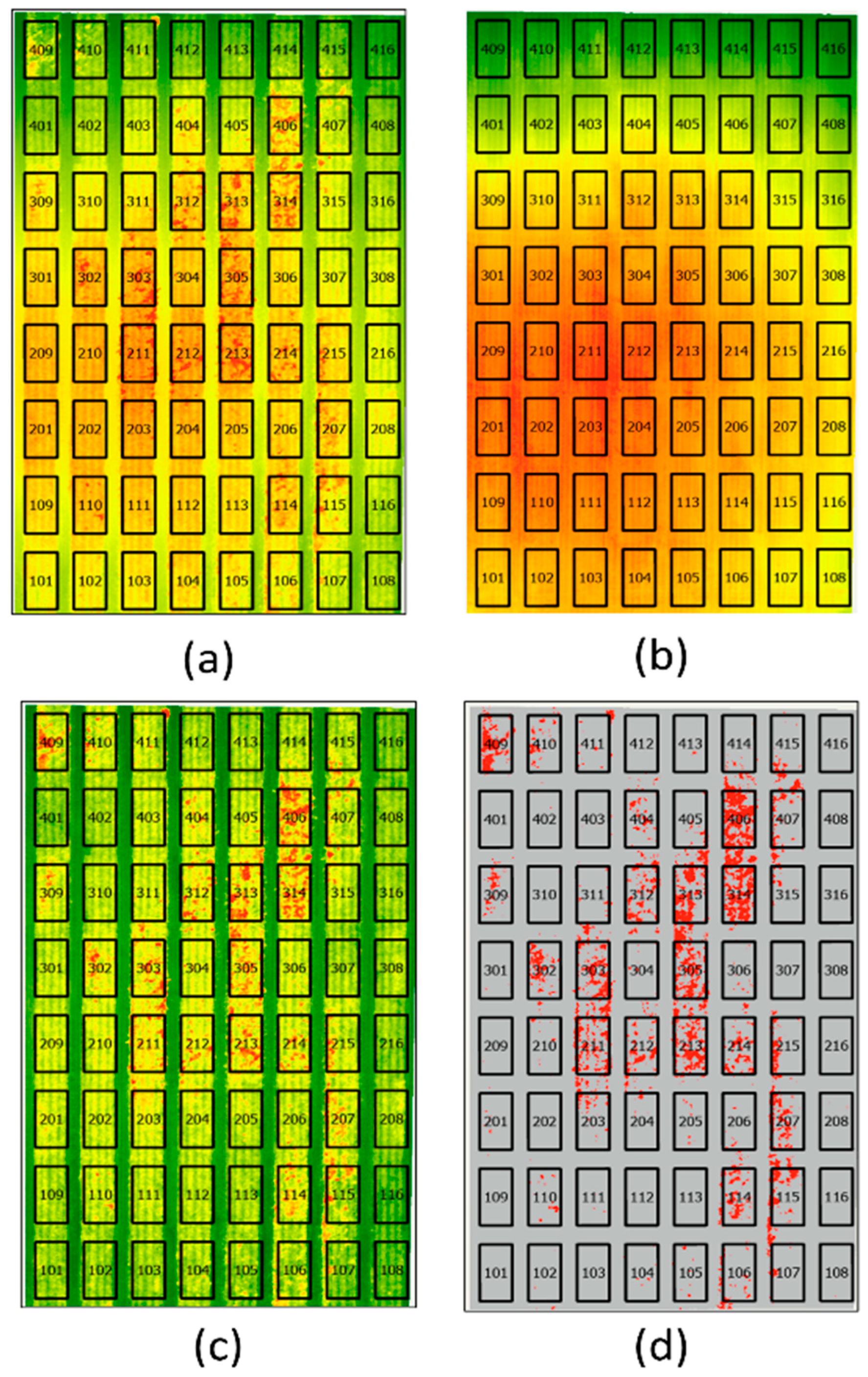
Figure 1. (a) The digital surface model (DSM) prior to subtraction of the digital terrain model (DTM). (b) The DTM obtained from a flight conducted in early February, showing field-scale variation in topography. (c) The canopy height model (CHM), obtained by subtracting the DTM from the DSM. The colors shown in panels (ac) represent height on a relative scale, with red representing higher points and green representing lower points. (d) A CHM Mask (CHMM) layer showing the application of the mask at the chosen mask height. Here, the “weed” class, which corresponds to pixels above the mask height, is shown in red, whereas the non-weed class is in gray. Some interference from the bed ridges is evident.
Agronomy 15 02885 g001
Figure 2. (a) The orthomosaic was used as a reference to identify areas infested by PA and create accuracy assessment samples, which are shown as yellow and green polygons for weed and non-weed (SP) areas, respectively. (b) The CHMM layer depicting the same plots shown in panel (a), demonstrating the polygon samples, now with accuracy assessment points.
Agronomy 15 02885 g002
Figure 3. Histogram showing the distribution of the weed area as determined by the CHMM approach. The distribution is strongly over-dispersed and right-skewed, making it suitable to be modeled using a gamma distribution.
Agronomy 15 02885 g003
Figure 4. Conceptual diagram for the left-censored distribution of weeds detected by the CHMM approach in relation to the bell-curve shape of the normal distribution. Weeds below the mask height are not detected by the CHMM approach, which precludes a normal distribution and requires other approaches for modeling the variable as a response.
Agronomy 15 02885 g004
Figure 5. (a) Orthomosaic with accuracy assessment samples (green and yellow polygons for weed and non-weed, respectively) and red circles indicating areas with PA. (b) CHMM layer with a 5.1 dm mask height. (c) CHMM layer with a 5.5 dm mask height. Increasing the mask height has the effect of shrinking areas classified as weed and increasing the false positive rate for weed.
Agronomy 15 02885 g005
Figure 6. Simple linear regression of SP yield (total marketable, fresh weight) against CHMM weed area. Observations from unfertilized, unamended plots, which accounted for the significant differences due to the amendment type treatment, were removed as they simultaneously exhibited low weediness (per visual ratings and CHMM weed area) and low yield.
Agronomy 15 02885 g006
Table 1. Confusion matrix results for the mask heights tested. For a given class, the user accuracy indicates the rate of false positives, whereas the producer accuracy indicates the rate of false negatives. With respect to the weed class (i.e., pixels above the mask height), a false positive occurs when a true weed sample or “positive” is classified as non-weed, and a false negative occurs when a true non-weed sample or “negative” is classified as weed. The overall accuracy considers the classification rate for all classes, and the Kappa statistic accounts for accuracy occurring due solely to chance.
Mask Height (dm)User Accuracy (%)Producer Accuracy (%)Overall Accuracy (%)Kappa Statistic (Kc)
Non-WeedWeedNon-WeedWeed
4.882789161810.55
5.191729075860.64
5.597628788880.66
6.199518594870.59
Disclaimer/Publisher’s Note: The statements, opinions and data contained in all publications are solely those of the individual author(s) and contributor(s) and not of MDPI and/or the editor(s). MDPI and/or the editor(s) disclaim responsibility for any injury to people or property resulting from any ideas, methods, instructions or products referred to in the content.