Weed Detection: Innovative Hyperspectral Image Analysis for Classification and Band Selection of Site-Specific and Selective Weeding Robot

Abstract

Weeding in melon and watermelon fields requires selective and pinpoint operation because the crop plants are sensitive to herbicides and tend to grow on the ground in all directions. Hyperspectral images have high spectral and spatial resolution, enabling an object’s classification according to its spectral properties. Spectral band selection is a common practice with hyperspectral images, as it reduces the number of bands in use with only a minor effect on the results. This study’s innovative contribution is the development and validation of a practical methodology to simplify complex hyperspectral data for real-world robotic weed management. This includes the introduction of the ‘normalized crop sample index’ (NCSI) to guide band selection and the use of machine learning methods, which revealed a set of four spectral bands—480 nm, 550 nm, 686 nm and 750 nm—that hold sufficient discriminating information between weeds and watermelon crop. This minimal set of bands enables the simulation and future development of a low-cost, high-speed multispectral camera system. An XGBoost model showed the lowest misclassification error level of 2–14%. The selected spectral bands were used to extract single-band images from the hyperspectral cube. In these images, vegetation pixels were separated using a normalized difference vegetation index filter, and each pixel was classified into a crop or weed class. The classified pixels were grouped into segmented objects, and weeding points were selected, suitable for robotic pinpoint operation.

1. Introduction

Population growth and rising demand for quality agricultural products call for the production of the highest and best yields. Weeds are the number one cause of yield loss in some crops [1] and they can reduce the yield by around 45% [2,3]. Hence, their management is extremely important. Weeding in crops such as watermelon is conducted by non-chemical methods because these crops are sensitive to chemical treatment [4]. Non-chemical weed management focuses on preventative and direct physical weed-control methods [5]. Whereas preventative methods reduce weed germination and cultural methods improve crop durability, the direct physical weeding methods affect weed survival and robustness [6].

Recent developments in weeding mechanisms, such as low-energy electrophysical treatment [7], water jets [8], air-propelled abrasive grit [9,10], hot foam [11], mechanical systems [12] and more, enable highly accurate weed management while avoiding physical contact with the crop plants. This precision operation fundamentally relies on the first and most critical step: accurate and selective detection of the weed from the crop. Common methods to discriminate between crop and weed usually consist of the following phases: sensing, vegetation separation (segmenting) and classification [13]. Common RGB cameras use spatial data and morphological features for detection and classification; moreover, hyperspectral or multispectral cameras can increase the accuracy when spectral features are used. Hyperspectral imaging, with its hundreds of narrow bands, serves as a crucial research tool to identify the unique and subtle spectral differences between crop and weed, which may be missed by the broader bands of RGB cameras. These spectral differences provide features that are often more robust for classification than morphological features, especially when plants are young, overlapping, or morphologically similar. The key motivation for this study is to leverage the power of hyperspectral analysis to accurately locate the smallest subset of effective spectral bands. This selection will then enable the development of an efficient, low-cost multispectral camera system for real-time robotic applications, which is a major constraint for field deployment.

Modern classifiers of crops and weeds, using multispectral camera images, have been developed recently [14,15,16]. The images usually consist of four bands in the visible and near-infrared (VNIR) spectral range. A multispectral camera can produce sharp, high-resolution images at real-time speed, while reducing the computational power needed for the classification, resulting in lower costs. The normalized difference vegetation index (NDVI) is used to separate the vegetation from other objects in the image. For example, a vision-based classification system [15] used a random forest to classify sugar beet plants and weeds with a four-channel multispectral camera. Feature-based key point and object-based classification methods were employed, showing a 96% overall accuracy, segmenting plants and weeds based on object features. A convolutional neural network (CNN) method [17] was also used to classify sugar beet plants and weeds, in two stages: the first was removal of the background with a fast-segmenting network (sNet), based on NDVI; the second was classification of the vegetation pixels with a more complex classification network (cNet). The two-stage method had an accuracy of 95–98% with a processing time of 0.93 s, compared to 92–96% accuracy and 23 s for the classification network alone. These studies typically focus on pixel- or object-level classification accuracy.

Hyperspectral imaging is globally recognized as a powerful tool in precision agriculture, offering the unique capability to map subtle biochemical and biophysical properties of vegetation that are invisible to the human eye or standard cameras. This is crucial for tasks like early disease detection, nutrient monitoring, and, as in this study, high-accuracy species classification across various crops. Other approaches use hyperspectral camera images with hundreds of narrow bands to classify crops and weeds. Zhang et al. [18] presented a method for automated selection of spectral features from a hyperspectral image to differentiate rice from weeds. The data were collected with a hyperspectral camera with 512 narrow bands in the range 380–1080 nm. The 800-nm channel was used as a primary mask to select the crop leaf. After de-noising by wavelet transform, a successive projection algorithm (SPA) was used to select spectral features (bands). The SPA selected the six most important spectral features (705 nm, 1007 nm, 735 nm, 687 nm, 561 nm and 415 nm, ordered by importance). With the six SPA bands, a weighted support vector machine (SVM) model was used to achieve 100%, 100%, and 92% recognition rates for barnyard grass, weedy rice, and rice, respectively. In Lauwers et al. [19], three classification models were used to distinguish between Cyperus esculentus weed and clones of morphologically similar weeds: random forest, regularized logistic regression and partial least-squares (PLS) discriminant analysis. Regularized logistic regression performed better than random forest or PLS discriminant analysis and was able to adequately classify the samples. The classification models were used on a hyperspectral reflectance dataset in the range of 500–800 nm. A low-cost multispectral camera based on four-band classification was used to simulate the results, and the simulated model classification accuracy was over 97%. In Diao et al. [20], a corn and weed classification was conducted by a spatial-spectral attention-enhanced Res-3D-OctConv model. The 350 spectral bands were reduced to four by principal component analysis, and the data were used by the model to classify the images. The model showed overall accuracy above 98% in the classification of the corn and weeds.

Many studies [21] have shown that band selection from hyperspectral data is very important to improving results. Band selection is based on the removal of highly correlated bands. Band selection also reduces the computational power needed for hyperspectral data processing. Various methods for selecting the most important spectral bands, such as linear discriminant analysis (LDA) [22], SVM [23], SPA [18] and random forest out of bag (OOB) [24] among others, are commonly used to reduce the number of bands. In the area of weed detection, spectral vegetation indices or image spatial indices have been used in many studies to classify vegetation [18,25].

Despite the promising high accuracy reported in the recent literature for crop and weed classification (e.g., 92–100%), two critical challenges remain for practical field implementation, particularly in crops like watermelon. First, a major challenge in watermelon cultivation is the need for extremely selective, pinpoint weed management, as the crop is sensitive to treatment and spreads in all directions on the ground, making standard weeding tools and methods unsuitable. The classification must be highly accurate and robust enough to avoid crop damage in close proximity. Second, many high-accuracy studies rely on full hyperspectral data with hundreds of bands, which demands significant computational power and specialized hardware, resulting in high costs that prevent wide-scale deployment on robotic platforms and are impractical for commercial use. Therefore, the critical issue is not simply achieving high accuracy but achieving high and robust accuracy with the minimal resources required for a cost-effective, real-time robotic system. This necessitates a precise methodology for spectral band selection.

The primary goal of this study was to find the most effective spectral bands for detecting weeds within a watermelon cultivation area [5]. To achieve this, an innovative and practical methodology was devised. The novelty of this approach lies in three critical aspects: first, the introduction of the ‘normalized crop sample index’ (NCSI), a new spectral analysis tool designed to simplify complex hyperspectral data for enhanced separation of two green vegetation types; second, the strategic use of conventional machine learning models for their ability to transparently and accurately select a minimal set of spectral bands from the original 840 bands in addition to optimize the classification performance; and third, the validation of this reduced spectral subset to enable the creation of a low-cost multispectral camera system for real-time robotic weed management. The objective was to identify a specific spectral range and the minimum number of bands that would be instrumental in the creation of a multispectral imaging system for weed detection.

As a result of careful consideration, the four most beneficial spectral bands were chosen, aligning with contemporary weed detection methodologies. It is important to note that this research forms a segment of an ongoing project dedicated to the advancement of a robotic weeding system.

2. Materials and Methods

The research comprised three main phases: firstly, conducting an experiment to collect hyperspectral data; secondly, performing band selection based on the spectral characteristics of the plants; and lastly, identifying potential weeding points (tool–weed contact points).

2.1. Experiment

An experiment was conducted in a commercial plot of watermelon (cv. Malali) where the common naturally grown weed population is of the genus Convolvulus. Hence, the focus of the study was on the Convolvulus as a weed. The plot was not weeded during the experiment for a period of 7 weeks from seeding. Hyperspectral images were collected from different regions of interest (ROIs) in the plot, which had both crop and weed plants. Each ROI was about 0.8 m long and between 0.4 and 1.2 m wide, depending on the growth stages of the crop and weed. Images were taken on three different dates in May and June 2019. On each measurement day, several crop rows were selected, and about eight ROIs were captured along 30 m in each row. The first measurement was conducted two weeks after seeding.

2.2. Experimental Apparatus

The data was collected using a hyperspectral camera, mounted on a custom data-collection cart (Figure 1a). The camera, a push-broom hyperspectral camera, VNIR HS (Specim, Oulu, Finland) with 840 spectral bands in the range of 395–1005 nm, a spectral resolution of 0.7 nm and spatial resolution of 1600 pixels, was attached to a rotary motor, Rotary (Specim, Oulu, Finland) (Figure 1b). The rotary motor was mounted on a cart, designed and built for the experiment at the Institute of Agricultural Engineering. The rotary motor was positioned at the front of the cart, at a height of 1.2 m above ground and at a 30-degree angle relative to the horizon. The motor rotated the camera at a constant speed, facilitating the line scanning process, where the camera direction traverses from one side of the Region of Interest (ROI) to the other. A sheet of square-patterned A4 paper (Figure 1c) was used as the “black and white” reference for the spectral reflectance and as a scale.

2.3. Data Acquisition

At each visit, about 25 ROIs were captured. Each ROI (Figure 1c) consisted of crop plant, weed, soil, the “black and white” reference paper and other objects in the field, such as stones and dry crop material from the previous season. The hyperspectral camera captures images line by line (pushbroom), with each line composed of a 1600 × 840-pixel frame, 1600 spatial and 840 spectral pixels. To capture a full image, the rotary motor start and end positions were set according to the stage and size of the plants of each ROI. The frame rate was set to 20 frames per second, and the number of lines varied between 1000 and 3000 according to the start and end positions. Hence, each ROI capture time was between 50 and 150 s. In addition, the hyperspectral data were presented as “pseudo RGB”, where specific narrow band channels were used to create a common “RGB” image look-alike. The bands for the pseudo RGB image were 486 nm for blue, 550 nm for green and 686 nm for red from the VNIR camera (Figure 1c).

2.4. Data Pre-Processing

The hyperspectral image pre-processing procedure presented in Figure 2 was based on 26 selected images (ROIs) from the three visits, defined as day 1, day 2, and day 3. The images were labelled and studied using custom software that was developed in-house.

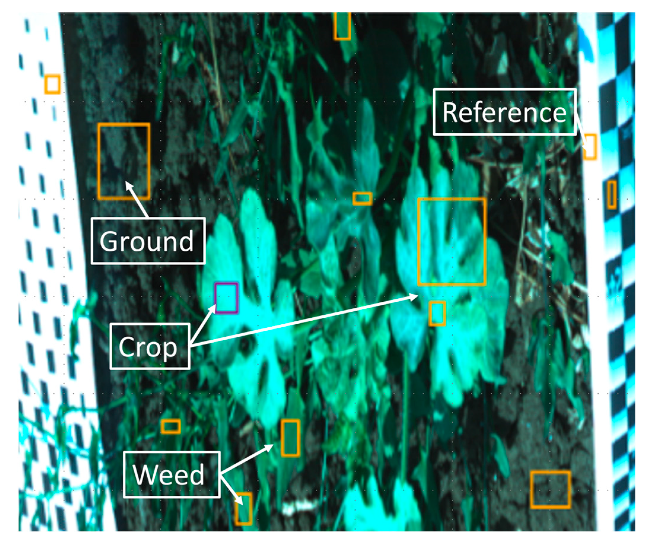
The selected hyperspectral images were used to extract each of the spectral bands from the image. Three single-band images were used to display a pseudo RGB image. Based on the pseudo RGB image and selected bands, several objects in the images were marked with rectangular frames and labelled as crop stem, crop leaf, weed, weed flower, “black and white” reference paper, and soil classes. The labels of crop stem and crop leaf were combined into a single class labelled ‘crop’. An example of a labelled ROI image is given in Figure 3. The dataset for the classification models consists of the crop and weed labelled frames from the selected images, and for each pixel in the labelled frames, a vector of the spectral reflectance was extracted from the hyperspectral image. In all, 572 labelled frames of crop and weeds were extracted from the data. The frames contained 55,639 pixels labelled as crop and 40,389 pixels labelled as weeds.

2.5. Spectral Data Analysis

The crop and weed labelled frames were used to inspect the spectral response of each population (crop and weed) by taking the mean value of all of the pixels in each labelled rectangle as the intensity of each band.

2.6. Classification Models with Band Selection

To classify crops and weeds while reducing the number of spectral bands captured by the VNIR camera (Specim, Oulu, Finland), we used five distinct classification models: (i) Linear Discriminant Analysis (LDA), (ii) Logistic Regression, (iii) Partial Least Squares (PLS), (iv) Random Forest, and (v) XGBoost [26]. These models also served the dual purpose of band selection, with the goal of narrowing down the pool of 840 spectral bands into four. The target of four spectral bands was selected based on engineering constraints and performance requirements. It is common in relatively low-cost commercial multispectral cameras and represents a balance between spectral information for high accuracy and minimal data for low computational cost and real-time operation in a robotic system. Two approaches were employed for band selection: “bottom up,” primarily utilizing two-band analysis, and “top down,” commencing from the complete set of 840 bands.

LDA (i) and Logistic Regression (ii) utilized the “bottom up” approach in a two-step process. The first step was to find a combination of two bands that minimized misclassification error. The second step used an iterative greedy approach: within each iteration, a single spectral band was added to reduce the misclassification error. In the first step, to reduce the computation time and avoid selecting adjacent bands, the spectrum of 840 bands was reduced to 84 bands with equal distribution along the spectrum (with approximately 7 nm spacing between spectral centres). On the reduced subset of 84 bands, a two-band analysis was conducted to generate a matrix of misclassification error levels, known as the “lambda–lambda graph”. For each pair of bands, the misclassification was found by either LDA (i) or Logistic Regression (ii). The misclassification matrix was composed in the following manner: each cell outside the main diagonal holds the misclassification error of two bands together. The main diagonal holds the misclassification error of a single band, leading to a total of 7056 combinations that were calculated. From the misclassification error matrix, the two bands that showed the lowest error were selected as base bands for the second step, the greedy approach. The greedy approach, which utilizes a widely accepted heuristic technique for local optimization, was conducted iteratively. A single iteration of the greedy approach compared the misclassification error of the base bands with that of a single band from the 840 bands of the full spectrum. The band that reduced the misclassification error the most was added to the base bands for the next iteration. The algorithm stops once the misclassification error reduction is small or once the desired number of bands is reached. In this study, two more bands were added within the second step to reach a total of four bands.

PLS (iii), Random Forest (iv), and XGBoost (v) followed the “top to bottom” approach, utilizing all 840 bands in their operation. Each of these models calculated a unique contribution score for each spectral band, representing the band’s significance as a feature in the model.

PLS (iii): PLS discriminant analysis is a versatile statistical method renowned for its ability in both classification and dimension reduction. In our context, it calculated Variable Importance in Projection (VIP) scores for each band. These VIP scores measured the cumulative importance of each band when considered in conjunction with all other bands. The VIP scores were instrumental in band selection, guiding the process.

Random Forest (iv): The Random Forest model, an ensemble of decision trees employing majority voting for classification, produced feature importance scores for each spectral band. These scores, generated using the Out-Of-Bag (OOB) method, reflected the band’s importance within the learning process of the algorithm. The bands with higher feature importance scores were prioritized in the “top down” selection process.

XGBoost (v): Operating on the principle of tree boosting and gradient boosting, the XGBoost model constructed a collection of boosting trees. During its learning process, XGBoost computed a ‘gain’ score for each spectral band, which gauged the band’s contribution to improved classification accuracy. The ‘gain’ score was the criterion for the “top down” band selection.

All classification models were implemented and trained using Python 3.10 with the scikit-learn and XGBoost libraries. For all models, a grid search hyperparameter tuning procedure was performed to optimize performance, focusing on minimizing the overall misclassification error. The computing environment used for all training and analysis consisted of a desktop PC with an Intel i7-9700K processor and 32 GB of RAM, running Windows 10. For each model, the key hyperparameters tuned during the grid search were as follows: LDA model: solver type (‘svd’, ‘lsqr’, ‘eigen’) and shrinkage parameter; Logistic Regression model: regularization strength (C) and penalty type (‘l1’, ‘l2’); PLS model: number of latent variables; Random Forest model: number of estimators (trees), maximum tree depth, and minimum samples per leaf; and XGBoost model: number of estimators (100–1000), maximum tree depth (2–8), learning rate (0.01–0.3), subsample ratio, and column sampling rate per tree. Furthermore, to validate the classification, a k-fold cross-validation was conducted with five folds. The k-fold cross-validation was used for all the models in each fitting process.

To ensure that the selected bands contributed meaningfully to classification, a spectral distance of at least 20 nm was maintained between the chosen bands. This precaution was taken because neighbouring bands tend to be highly correlated, potentially causing redundancy and describing the same spectral phenomena. Following the band selection process, a subset comprising the chosen bands was employed to train the classifiers. The models were rigorously tested on data from each visit day individually, as well as on the aggregated dataset spanning all days. Each model underwent training and fitting using 80% of the data and was then evaluated on the remaining 20%. Importantly, in each training session of each algorithm, multiple train–test splits were employed to ensure robustness in the model’s performance assessment.

2.7. Weeding-Point Selection

The weeding point is considered as the physical contact point between the weeding tool electrode and the weed. The selection of weeding points involves a structured image-processing workflow, encompassing four key steps:

(i) NDVI Vegetation Mask Application: Initially, an NDVI vegetation mask was applied. This mask identified living plants by utilizing two specific bands (686 nm and 750 nm) to separate the plant pixels from the background. Subsequent image processing steps focused exclusively on this masked vegetation data.

(ii) Pixel Classification: Classification was conducted using grayscale images of specific spectral bands from the hyperspectral VNIR camera. In this study, four spectral bands were selected by the classification models. Each of these bands contributed a set of four images used for classification. Every pixel within the vegetation mask was represented as a four-value vector. Each classification model was applied to this labelled data, generating a classification image for each of the four spectral bands. A pixel-wise majority vote from all the classification models produced a comprehensive classification mask distinguishing between crop and weed.

(iii) Segmentation of Contoured Objects: To ensure the separation of crops from weeds, a distance had to be maintained between the crop and the weeding tool. Achieving this involves enlarging the crop objects through morphological dilation and removing all weed pixels within the expanded crop area. This segmentation process unfolded in two steps: first for the crop population and then for the weed population. For the crop population, the steps included noise filtration, contour detection, and contour shape dilation to create a crop mask. For the weed population, the process commenced with the subtraction of the crop mask and then proceeded with noise filtration, contour detection, and contour shape erosion. This resulted in a segmented image, effectively distinguishing crop and weed objects.

(iv) Selection of Weeding Point: The final step involved selecting weeding points while maintaining a safe distance from the crop plants. A minimal distance of approximately six cm was preserved, considering data analysis that indicated this to be less than the average distance between two weed plants, effectively treating them as the same plant. To ensure this distance, the image was divided into small sections, approximately 6 × 6 cm in size, by averaging the values of the surrounding area. Sections containing crop values were excluded, retaining only the segments with weed presence. The image with the isolated weed section was then divided into overlapping tiles. The number of weed pixels within each tile was calculated. These tiles were then ranked based on the quantity of weed pixels they contained, without any overlap. Weeding points were selected by choosing tiles with the highest weed pixel count, thereby facilitating precise weed removal.

3. Results

3.1. Spectral Data Analysis—Development of the ‘Normalized Crop Sample Index’ (NCSI)

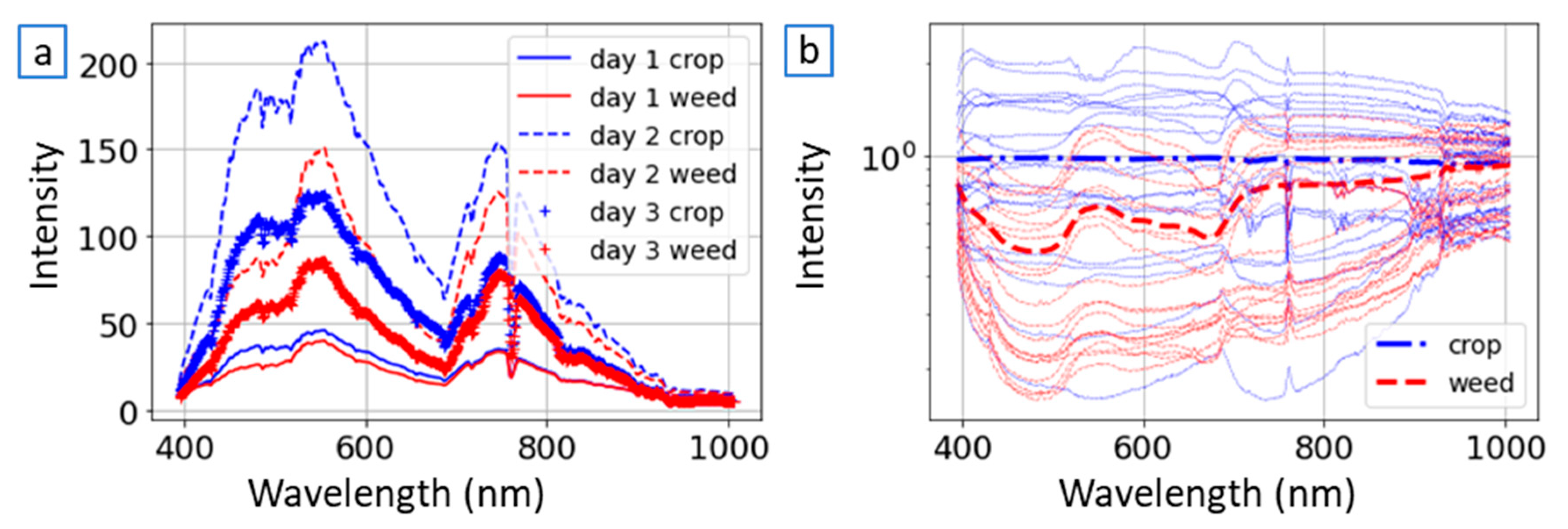
The spectral response of the labelled frames of crop and weed classes from the ROIs images was analyzed, as seen in Figure 4. Each labelled frame out of the 572 samples, represented as a vector ${\overrightarrow{\lambda }}_i$ of the mean intensity values of the pixels of the frame in each band. The NCSI, denoted as ${\mathsf{\Lambda }}_{\left(i\right)}$ (Equation (1)), was used for the normalization of the samples. The NCSI uses a normalization vector ${\overrightarrow{\lambda }}_{mean}$, which can be one crop pixel’s spectral values, one crop-labelled frame’s mean spectral values, or another selection of $n_j$ samples from the crop population. Therefore, each element ${\overrightarrow{\lambda }}_{{mean}_j}$(Equation (2)) is the mean spectral reflectance of the $n_j$ samples, used for the normalization of band j in ${\overrightarrow{\lambda }}_{mean}$ normalization vector. The $n_j$ samples represented as ${\lambda }_{i,j}$ where i considered to be one of the ${\overrightarrow{\lambda }}_i$ vectors and j the specific spectral band. The NCSI, when applied to one labelled frame, divides the spectral response of a sample ${\overrightarrow{\lambda }}_i$ with the normalization vector ${\overrightarrow{\lambda }}_{mean}$element wise. In the study, ${\overrightarrow{\lambda }}_{mean}$ was developed with samples of the crop population.

$${\mathsf{\Lambda }}_{\left(i\right) }={\displaystyle \frac{{\overrightarrow{\lambda }}_i}{{\overrightarrow{\lambda }}_{mean}}}$$

(1)

$${\overrightarrow{\lambda }}_{{mean}_j}={\displaystyle \frac{ {\sum }_{i=1}^{n_j}{\lambda }_{i,j} }{{\mathrm{n}}_j}}$$

(2)

The underlying principle of the NCSI can be simplified in the case that ${\overrightarrow{\lambda }}_{mean}$was selected as specific ${\overrightarrow{\lambda }}_i$ vector from the dataset. In this case, the expectation is that when the NCSI is applied to a different sample of the same type of plants, the watermelon crop in the study, the index values will exhibit a relatively straight and levelled pattern parallel to the straight line that represents the chosen sample. Conversely, the NCSI spectra of weed samples are anticipated to demonstrate fluctuations, as seen in Figure 4b. The average spectral reflectance for each population for each trial day is seen in Figure 4a, while the bold representation in Figure 4b depicts the average NCSI spectral reflectance (as defined in Equation (1)) across all samples. Upon analyzing the NCSI spectral response, specific characteristics were observed for the crop-labelled frames within the designated ROIs. Specifically, within the spectral range of 450 nm to 690 nm and 750 nm to 900 nm, the spectral response remained generally stable, forming a consistent line. However, a marked transition in the spectral response was identified in the range between 690 nm and 750 nm. In contrast, the normalized response of the weed samples displayed fluctuations within the range of 450 nm to 690 nm, with a distinct change occurring between 690 nm and 750 nm. Other portions of the spectral response were found to be unstable due to the sensor’s limited signal-to-noise ratio in these specific spectral bands. In certain instances, particularly those involving low intensity (such as on trial day 1) or suboptimal selection of the crop sample frame, fluctuations were observed in the crop response. While variations were noticeable in the weed samples based on the selection of different crops, the regions corresponding to local minimum and maximum responses remained consistently positioned within the same spectral regions.

The four bands that were manually selected in the spectral analysis were in the areas of the local minimum and maximum points of the NCSI spectral response of the weed, and at the edges of the sharp spectral change seen between 690 nm and 750 nm. The four selected bands were: 480 nm, 550 nm, 686 nm and 750 nm. This set of four bands was defined as the ‘NCSI band selection’, to be compared in all classification models as the reference selection of bands for the model.

3.2. Classification and Band-Selection Models

The spectral response of each pixel in the crop and weed-labelled rectangles was used to train five classification models: greedy LDA (i), greedy logistic regression (ii), PLS (iii), random forest (iv) and XGBoost (v). For each pixel, an 840-value vector of the intensity of each spectral band was extracted, for a total of about 100,000 pixels.

The models were trained for each trial day separately and on all days together. For each day, the spectral response of each pixel was normalized using the NCSI, where ${\overrightarrow{\lambda }}_{mean}$is the vector of the mean response of all crop pixels on the same day. The baseline of the misclassification error level was assessed on the dataset of labelled pixels with 840 bands. All models showed similar results, with misclassification error levels of about 5%, 1.5% and 2% for days 1, 2, and 3, respectively. For each model, the method specified in Section 2 was used to find the set of four bands with the lowest misclassification error level. As mentioned in Section 2, a k-fold cross-validation was used for all training of the models. The spectral reflectance of the measurements on each day differed in intensity due to camera calibration and the changes in environmental conditions (e.g., varying sunlight intensity and angle), where day 2 had the highest intensity and the camera calibration was sharp and detailed, and day 1 had the lowest intensity and was the least detailed. The diverse levels of intensity during and between the days posed a challenge for the band selection of each model, because the bands that contributed most on each day differed with respect to the intensity difference. The successful normalization of the spectral response using the NCSI, which utilizes the mean crop response of the same day for normalization, alleviated the effect of these environmental changes, demonstrating a path toward robust daily operation. Furthermore, during the band selection procedure, a deliberate exclusion was made with respect to the spectral region exceeding 850 nm. This exclusion was motivated by the presence of a notably low signal-to-noise ratio within this specific spectral range in the specific outdoor conditions in which we took the images. This limitation is generally tied to the sensitivity of the VNIR sensor at the higher end of its range and the specific lighting/field conditions. This limitation could potentially be mitigated through the use of cameras with improved sensitivity at higher wavelengths or by implementing more sophisticated spectral pre-processing techniques, such as advanced filtering or specific sensor calibration for the NIR range.

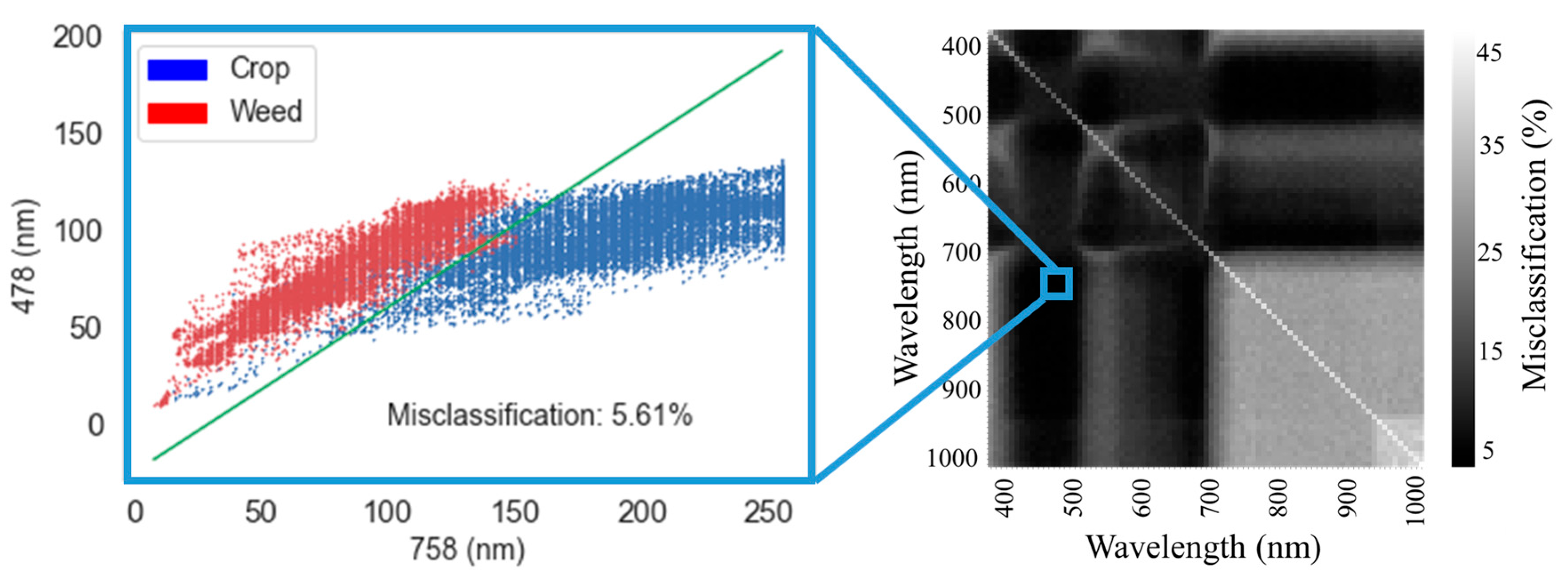
For the LDA (i) and logistic regression (ii) models, the bands that reduced the misclassification error level the most over all 3 days were selected according to the greedy selection algorithm. In the first stage of the algorithm, two-band analysis, as shown in Figure 5, produced a matrix of misclassification error rate for each of the two bands in the matrix. The two-band misclassification matrix is characterized by regions where the misclassification was low (black); these areas of the matrix indicate that multiple selections of specific two bands can produce low misclassification error. Notably, the main diagonal of the matrix shows high misclassification errors, occurring when the same band was selected twice, since analyzing a single band effectively employs only a single feature. 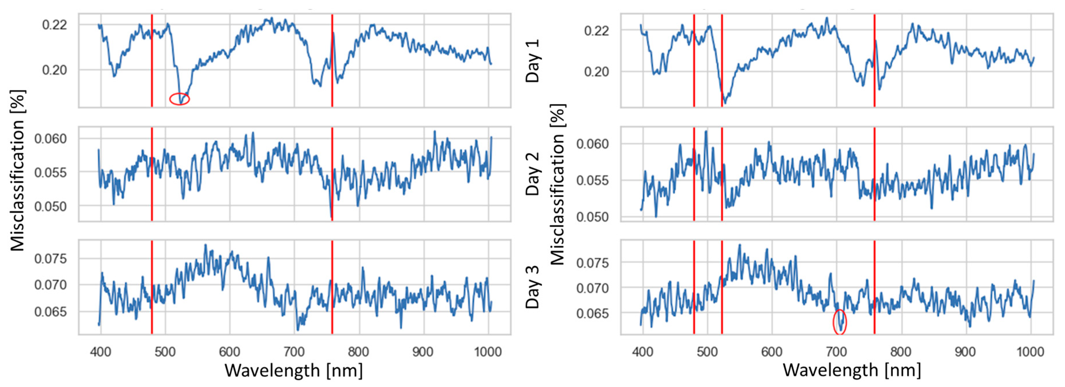Figure 6 shows the process of the greedy selection and highlights the bands chosen for the LDA model. This selection process commenced by establishing a set of base bands (represented by vertical red lines), which were the bands selected in the two-band analysis. For every consecutive band, a classifier was trained to assess the contribution of that band toward reducing misclassification errors. The most advantageous band, optimizing misclassification rate reduction across the three days, was determined by identifying regions where misclassification was minimal while maintaining a spectral distance of 20 nm between the base bands. Furthermore, in the band selection procedure, the introduction of the third and fourth bands was guided by the lowest misclassification error rates observed on days 1 and 3, respectively, due to their significant contributions. Consequently, for day 2, the addition of these bands resulted in a comparatively minor reduction in misclassification when contrasted with the base bands.

In the case of the PLS (iii), random forest (iv), and XGBoost (v) models, the bands that were chosen for inclusion in the models were those that demonstrated substantial feature importance, as outlined in Section 2 specific to each model. As shown in Figure 7, the XGBoost model’s band selection process is illustrated.

The misclassification error level of the data from all days for the four bands selected by each model was 12% on average, whereas the misclassification error level when using the NCSI reference bands was between 11% and 14% (

Table 1. Four-band misclassification error level of each model based on the selection of four bands from the NCSI spectral analysis (480 nm, 550 nm, 686 nm, and 750 nm) and on the selection of four bands according to each model-specific method. The bold figures represent the best results for each day and all days data. The bands selected by each model are presented in Table 2.

Model	Day 1	Day 2	Day 3	All Days
NCSI bands
LDA	0.201 ± (0.003)	0.051 ± (0.001)	0.080 ± (0.004)	0.141 ± (0.003)
Logistic regression	0.183 ± (0.003)	0.037 ± (0.002)	0.064 ± (0.003)	0.134 ± (0.004)
PLS	0.203 ± (0.003)	0.056 ± (0.001)	0.074 ± (0.002)	0.135 ± (0.003)
Random forest	0.145 ± (0.002)	0.028 ± (0.002)	0.050 ± (0.001)	0.110 ± (0.004)
XGBoost	0.142 ± (0.004)	0.022 ± (0.001)	0.050 ± (0.001)	0.108 ± (0.003)
Model-method bands
Greedy LDA	0.182 ± (0.003)	0.049 ± (0.002)	0.047 ± (0.003)	0.119 ± (0.003)
Greedy logistic regression	0.175 ± (0.004)	0.035 ± (0.002)	0.042 ± (0.003)	0.120 ± (0.004)
PLS—VIP	0.169 ± (0.003)	0.051 ± (0.001)	0.046 ± (0.003)	0.120 ± (0.003)
Random forest—OOB	0.160 ± (0.004)	0.035 ± (0.002)	0.046 ± (0.002)	0.119 ± (0.004)
XGBoost—gain importance	0.144 ± (0.004)	0.022 ± (0.002)	0.052 ± (0.005)	0.109 ± (0.001)

). The random forest and XGBoost showed the lowest misclassification error levels with the reference bands selected by the NCSI; however, for the LDA, logistic regression and PLS, the model method of band selection gave better results than the NCSI reference bands. The set of four bands selected by the model-specific method tended to classify better on days 1 and 3 because the selection method was influenced by the reduction in misclassification error level, which was larger for those days.

Overall, the misclassification error using the four bands for pixel classification was below 5% for most days, but higher than the baseline levels found with all 840 spectral bands. Moreover, while it is not crucial to calibrate the cameras properly to achieve less than 12% misclassification error over all days, for day 2, where the images were the most detailed due to good camera calibration, the misclassification was lower than 2% (Table 1).

Investigation of the four-band combinations selected by the models (

Table 2. Selection of bands by each model (Lazar and Bechar, 2021) [5].

Model	Band 1 (nm)	Band 2 (nm)	Band 3 (nm)	Band 4 (nm)
NCSI—manually selected	480	550	686	750
Greedy LDA	478	529	705	758
Greedy logistic regression	478	522	677	758
PLS	470	527	705	759
Random forest	484	552	758	813
XGBoost	485	554	668	735

) showed that most of the bands were found near the NCSI manually selected bands. This indicates that the NCSI explains the spectral differences through a simple interpretation of the data. In addition, the selection made by the spectral analysis consisted of bands that had been used in previous studies for plant classification [25].

3.3. Weeding-Point Selection

The weeding-point selection consisted of five main stages: the first was to extract the image from the hypercube, followed by the four stages mentioned in Section 2. Figure 8 shows the workflow of the process.

3.4. Image Classification with Four Bands

The hyperspectral images of the ROIs were used to classify the vegetation pixels in each ROI image into crop and weed. The classification was based on a four-band classification according to the selection of each method (Table 2). For each set of bands, four single-band images were extracted from the hyperspectral cube according to the selection of the classification model. Five sets of four single-channel images were extracted for the machine learning algorithm band selection. An additional set of four single-channel images was extracted for the NCSI manual band selection, resulting in six sets of images.

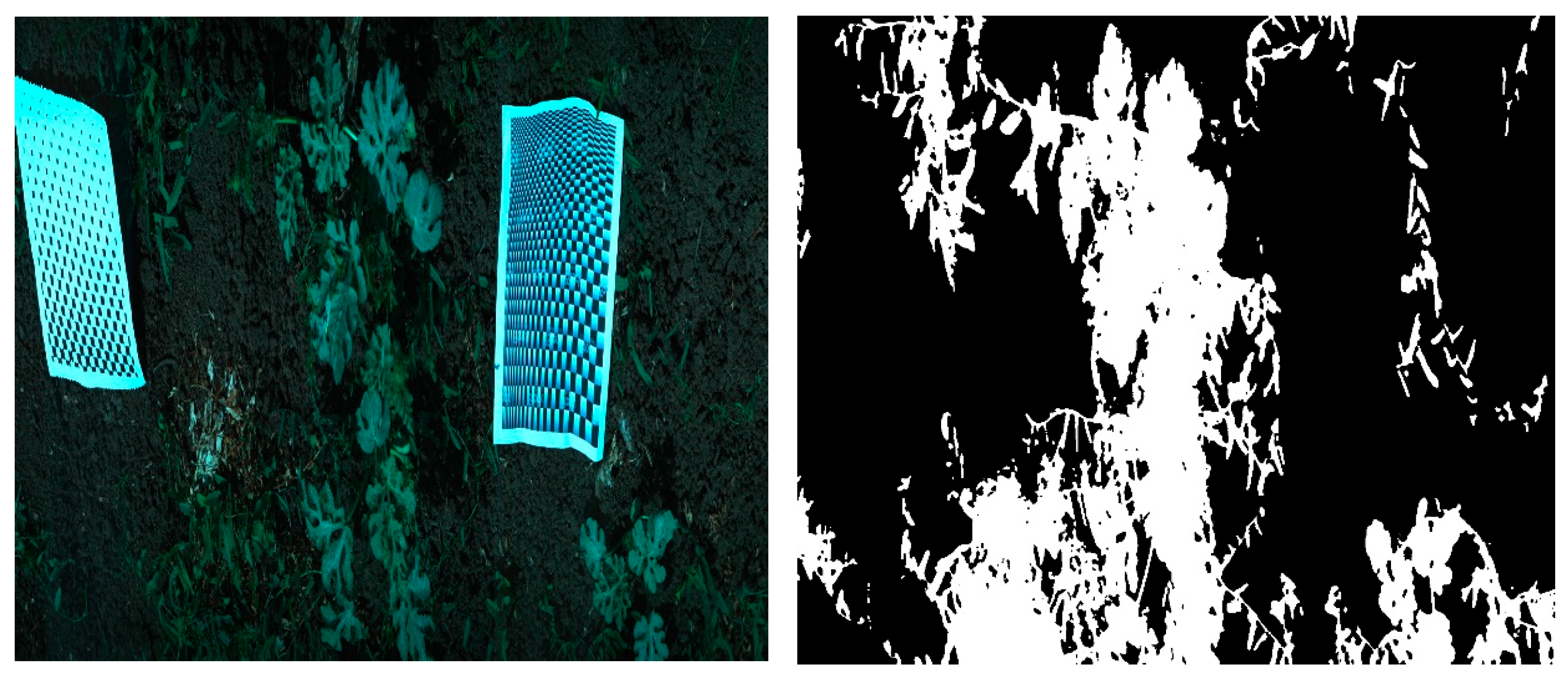
To separate the vegetation from the background, an NDVI filter was used with two of the four bands from the NCSI set—the 750 nm and 686 nm bands—to create a vegetation mask (Figure 9) of the ROI. Consistently, the same vegetation mask was used for all classification models to extract the pixels that represent vegetation for classification.

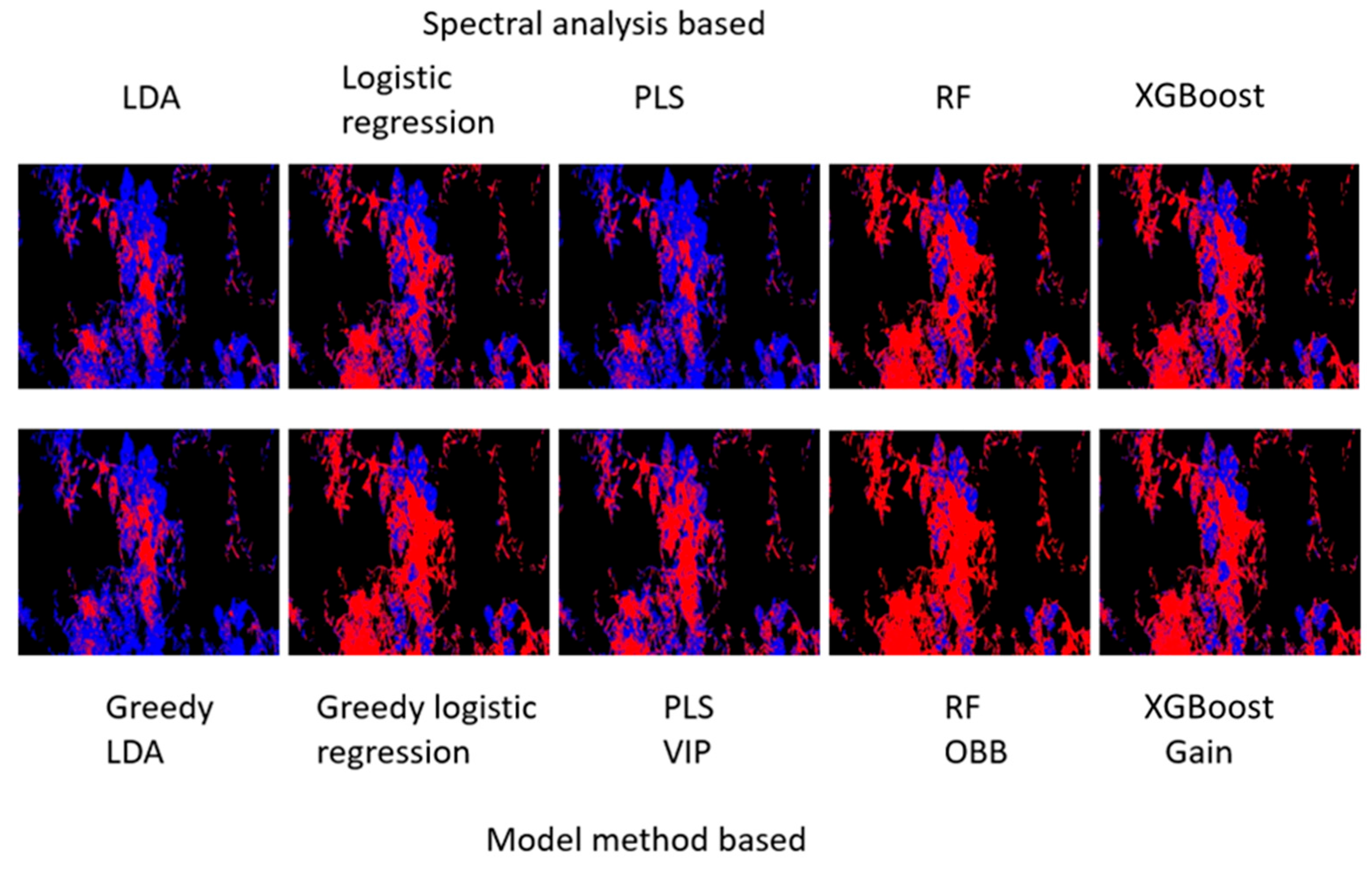
For qualitative assessment of the models, the six different sets were used, where each set of four single-band images was used for classification. Each vegetation pixel was classified 10 times, five times for the NCSI reference bands used by each classification model, and five times for the bands that were selected and used by the classification models (Table 2). The pixels were represented by ${\overrightarrow{\lambda }}_i$, which was a four-value vector, one for each band. The vectors of the pixels were classified by the models to produce 10 classification masks (Figure 10) of the classified pixels. The masks were produced by the classification models that were trained with data from the day on which the ROI image was taken. Inspection of the classification masks shows that all the classification models correctly classified most vegetation pixels. However, each mask differs in the classified pixels, with some pixels correctly classified and others misclassified.

Most misclassifications occur at the edges of vegetation objects, where there can be shading from other plants, resulting in a low spectral difference. Random forest and XGBoost tend to classify these pixels as weeds, whereas the other methods classify them as crop. To resolve the conflict between the classification mask, for each pixel, a majority vote of all 10 models was used to create a classification mask that reduces misclassification. Each pixel (x, y) in the majority classification image was considered a weed pixel if six or more (out of the 10) models classified it as a weed; otherwise, the pixel was considered to be a crop. Furthermore, the classification masks showed better results when the model training data were normalized using the NCSI, where ${\overrightarrow{\lambda }}_{mean}$ (Equation (2)) was calculated as the mean response of the crop-labelled pixels from the same day that the image was taken, and each vegetation pixel ${\overrightarrow{\lambda }}_i$ was normalized using NCSI ${\mathsf{\Lambda }}_{\left(i\right) }$ (Equation (1)).

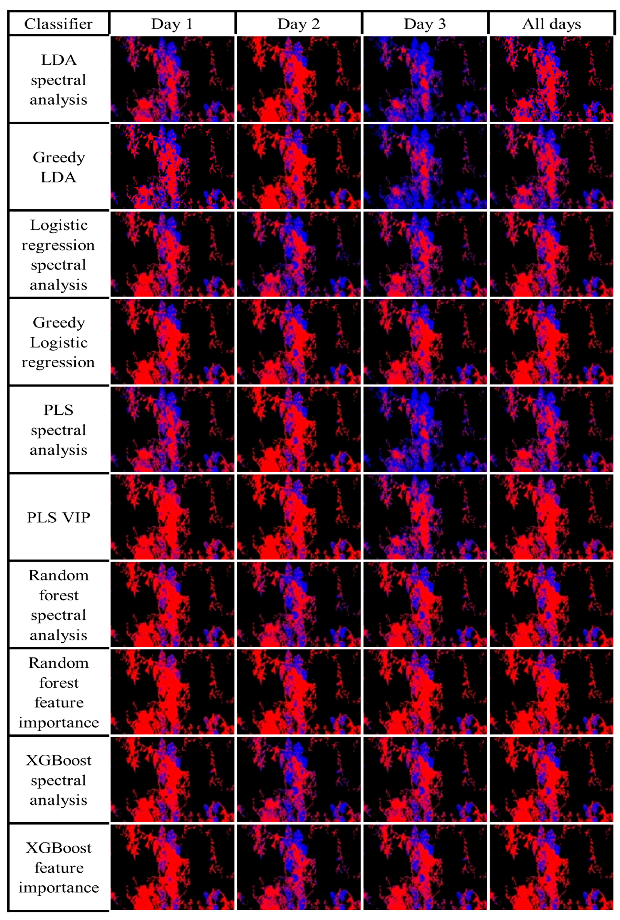
To investigate the classification quality when using data from different days to train the classification models, each ROI image was classified 30 more times for a total of 40 classification masks. For each day, 10 classification masks were trained only on that day’s data. An additional 10 classification masks were generated by models trained on data from all days. All 40 classification masks, 10 for each day and 10 for all days, are presented in Figure 11 to provide a more comprehensive understanding of the classification outcomes generated by each classifier. Inspection of Figure 11 shows that XGBoost and Random Forest produce robust classification for all the masks, while with the other models, the classification changes when using different day data. The assessment of the classification mask indicates that the best classification was achieved when using the same-day data for classification. However, using data from day 2, which showed the lowest misclassification error (Table 1), produced masks that correctly classified most pixels, indicating the possibility of achieving similar results with high-quality stored data.

The final image classification workflow, which relies on a majority vote across 10 classification masks derived from both the NCSI-selected and model-optimized four-band subsets, serves as an effective mechanism for error mitigation and maximizing robustness. The qualitative assessment of the classification masks clearly highlights the ability of the reduced four-band set to accurately differentiate vegetation, with most misclassifications occurring in challenging areas like plant edges or shaded regions. Crucially, the finding that normalization via NCSI significantly improves classification quality across the board underscores the index’s operational value, and the demonstration that high-quality, normalized data can yield correct classification even for unseen images suggests a viable path toward a generalized, high-accuracy model that requires only periodic, not continuous, field calibration.

3.5. Image Segmentation and Point Selection

The segmentation procedure is based on a majority vote classification mask. Using the algorithms presented in Section 2, the crop and weed objects were classified. Figure 12 shows the segmented objects, and the crop (blue) objects include some weed pixels, which are either between or near the crop pixels. The segmentation objective is to avoid weeding of the crop. In addition, weed objects are to be evaluated as smaller than the area of classified weed pixels, and are to be considered crop-free.

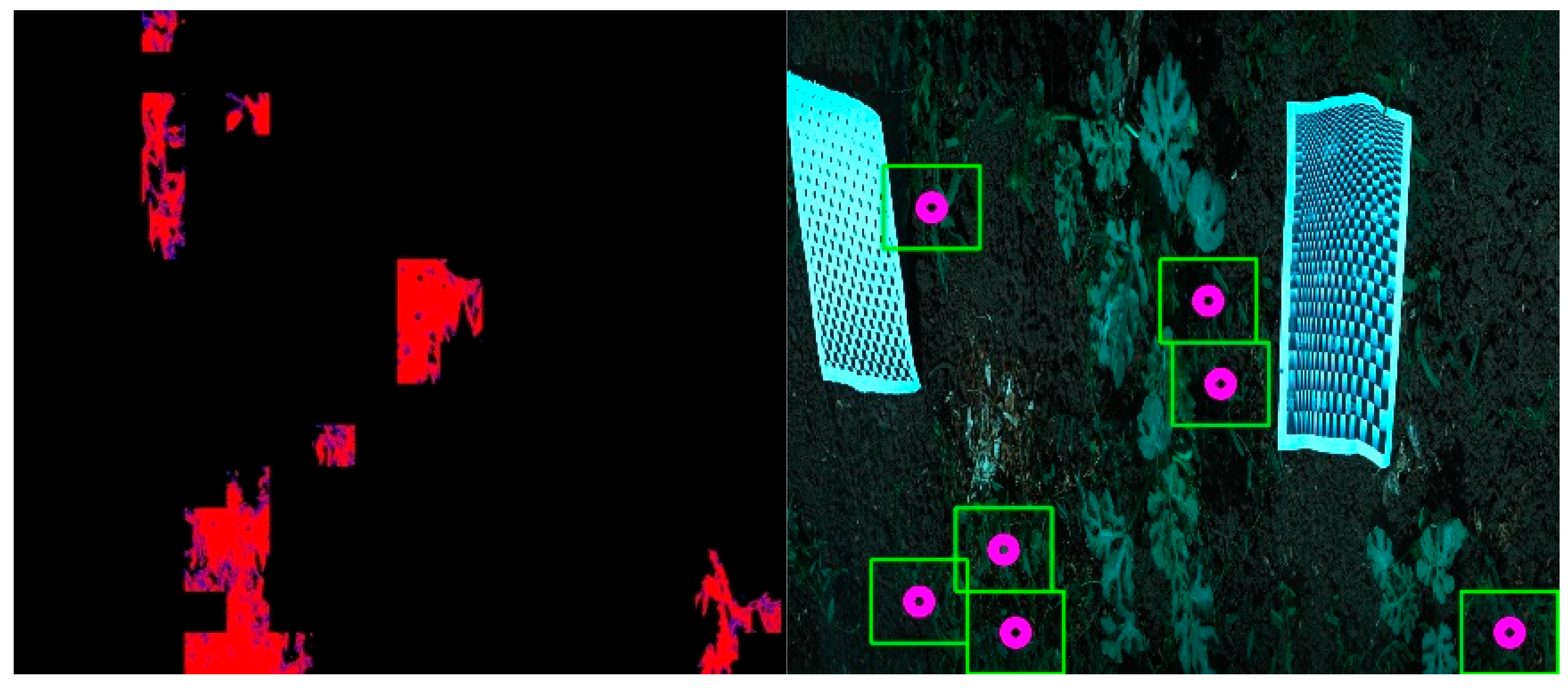
The segmented mask was resized by averaging to a small image of about 15 pixels in height, where each pixel represents about 6 × 6 cm, to find weed areas that are remote from the crop. In the small 15-pixel high image, pixels that had some crop (blue) values were disregarded. The result was a crop-free weed area image (Figure 13). The weeding points selected from the crop-free tiled image followed the distance rules and did not touch any of the crop pixels. All of the ROI VNIR hyperspectral images were used in this procedure, and weeding points were selected for each ROI image that contained weeds. An expert evaluation of the quality of the number and location of the weeding points found that all weeding point positions were weed pixels in the images and that it is sufficient for the process of handling intra-row weeds with pinpoint selection. However, the objective evaluation of final weeding-point selection accuracy, as well as metrics like detection time and rate of successful weed removal, requires further field-based research to be conducted using the algorithm in a commercial plot.

4. Discussion and Conclusions

A case study was conducted for the classification of cv. Malali watermelon crop and weeds of the genus Convolvulus. Four-band subsets selected from 840 bands of the VNIR camera (400–1000 nm) demonstrated that four-band subsets achieved sufficient accuracy for targeted weeding. This success was critically supported by the introduction of the Normalized Crop Sample Index (NCSI), a practical innovation that simplifies complex hyperspectral data for real-world agricultural use by normalizing the sample’s spectral response against the mean crop signature. This normalization effectively amplifies the subtle, vital spectral differences between the crop and the weed, minimizing the impact of day-to-day environmental variability. The NCSI proved a powerful, straightforward tool for feature engineering, as the four manually selected bands (480 nm, 550 nm, 686 nm, and 750 nm) precisely aligned with the index’s critical spectral inflection points and produced similar results, in terms of selected bands and low misclassification error, to those selected by five different machine learning models. The misclassification error levels were similar as well.

The NCSI is a novel contribution as it functions as a comprehensive spectral normalization tool, unlike a simple two-band spectral index such as the NDVI. The NDVI is primarily used for binary segmentation, separating all vegetation from non-vegetation. The NCSI, by contrast, normalizes the full spectral vector of an unknown plant against the average full spectral vector of a known crop sample. This process effectively minimizes external noise and variations due to illumination or camera calibration, which can cause intensity shifts across the spectrum. The NCSI’s main advantage is that the resulting normalized spectrum (Figure 4b) emphasizes the subtle spectral differences between the weed and the crop, transforming the problem from distinguishing between two similar absolute reflectance curves into classifying based on a distinct pattern of deviation from the crop’s baseline. This ability to simplify the interspecies difference across the full spectrum proved instrumental in manually identifying the optimal distinguishing bands.

It was found that the greedy LDA, greedy logistic regression and PLS are sensitive to the differences in daily conditions and to the band-selection method, as seen in Figure 11. The classification masks produced by those models show a high difference when the classifiers were trained on the same day or on different days. These models therefore operate with relatively lower performance when the training and testing images are from different days; on the other hand, random forest and XGBoost show robust performance even when the tested data are taken from days that differ from those of the training data. This robust performance of Random Forest and XGBoost, which are tree-based models, is likely due to their non-linear nature and their internal mechanisms for handling feature variance and outliers more effectively than linear models like LDA or Logistic Regression. They create multiple decision trees, which effectively average out the noise and variability present in the data collected across the different days, leading to a classification decision that is more stable and more robust than a single linear model. Overall, the use of random forest or XGBoost as classification models is preferred because the classification showed the overall lowest misclassification error level and was more robust across dynamic field conditions. This insight suggests that future robotic systems should prioritize the use of these robust, non-linear classification methods for reliable performance in dynamic, real-world agricultural environments and low-dimensional spectral features.

Due to the distinct spectral characteristics exhibited by crops as compared to weeds, the labelling process was efficient, requiring only a relatively small number of frames. Specifically, 572 frames were selected from 26 chosen ROI (Region of Interest) images to create the classifiers. These labelled rectangles were carefully chosen from the VNIR ROI images for each class. A modest amount of labelled data, approximately 100,000 pixels, proved to be more than adequate for training classification models that hinged on the four spectral bands. These models demonstrated a remarkable ability to classify unknown data with a high degree of accuracy. The spectral characteristics identified by the NCSI and selected bands are derived from the spectral contrast between the watermelon (cv. Malali) and the weed (Convolvulus). However, the developed methodology using NCSI is a universally applicable method to distinguish between melon (crop plant) and different types of weeds since it is normalized by the crop spectral signature. The machine learning for band selection is portable and can be adapted to different crop/weed species. The methodology developed in this context and the approach of working with a compact dataset could easily be adapted for use with different weed varieties. Periodic calibration, such as at the outset of each day or whenever environmental conditions undergo significant changes, could be facilitated by labelling a limited number of crop and weed plants and subsequently updating the classification models with real-time data. Furthermore, the quality of the camera calibration played a crucial role. In cases where calibration was suboptimal, as seen on day 1, certain classifiers exhibited superior performance in classifying unseen images. However, under conditions of good calibration, all the classifiers consistently demonstrated proficient image classification.

The final steps of image segmentation and weeding-point selection demonstrate the method’s transition from spectral science to robotic engineering. The segmentation algorithm, by aggressively prioritizing crop protection through dilation and weed-object erosion, generates distinct, crop-free weed objects suitable for physical intervention. The use of spatial averaging to create large (6 cm × 6 cm) tiles and then ranking them by weed pixel density effectively converts the pixel data into a discrete, manageable set of high-confidence treatment locations. This tiling process is the practical bridge between accurate classification and the constraints of a mechanical weeding tool, ensuring that the selected points are not only weeds but are also spatially isolated and dense enough to warrant a precision treatment, thereby completing the robust workflow necessary for a functional, selective weeding robot.

The study indicates that future application of a robotic platform equipped with a four-band multispectral camera may be able to detect and apply treatment for weeds in watermelon plots with pinpoint operation. Such a camera, which uses four narrow bands, can produce fast and accurate crop and weed detection with low cost and low computational resources in comparison to an 840-band hyperspectral camera. This is due to the significant reduction in data dimensionality from 840 to only four spectral bands, making real-time processing substantially easier and enabling the use of less expensive hardware. Further studies are required to determine the actual operational metrics, such as model response speed and power consumption, with reference to the weeding tool and the critical weeding period, and to increase the diversity of the crop and weed data.

The NCSI, with a minimal set of four bands, is highly effective for crop-weed discrimination. The key advantage of the NCSI approach lies in its simplicity and inherent spectral interpretability. By normalizing the spectral response of a sample against the mean crop signature, NCSI effectively isolates the subtle, differential reflectance characteristics critical for separating crop and weed. This approach demonstrated strong efficacy, as the NCSI-selected bands were consistently near the optimal bands identified by more complex, purely algorithmic methods like Greedy LDA, PLS, and XGBoost. In contrast, automated dimension reduction techniques, such as the Principal Component Analysis (PCA) used by Diao et al. [20] or the Successive Projection Algorithm (SPA) used by Zhang et al. [18], are effective for data compression but often yield spectral features that are linear combinations of the original bands, thereby losing direct physical interpretability. The SPA method, for example, selected six specific features [18], achieving high accuracy but necessitating a larger feature set than our target. The NCSI approach, by focusing on spectral inflection points derived from biophysical differences (chlorophyll absorption and cellular structure), provides a transparent, low-cost alternative to these automated methods. This transparency is crucial for the engineering development of a low-cost, multispectral camera system, confirming that the minimal four-band subset is sufficient for high-accuracy discrimination.

A limitation of this study is that although NCSI was designed to cope with several weeds, it was examined on a single crop-weed pair, which, while proving the methodology, limits the immediate universal applicability. Furthermore, while the model was robust, the data collection covered only three non-consecutive days. However, the models, particularly XGBoost, demonstrated a remarkable ability to classify unknown data with a high degree of accuracy with a modest amount of labelled data, alleviating the concern of a small training set size or potential overfitting. Future research should focus on three main directions: expanding the dataset to include greater diversity of weed species and crop growth stages; performing a direct, objective field validation of the entire robotic system to measure real-time operational metrics like detection speed and successful weeding rates; and, adapting the NCSI-based band selection methodology to other high value crops to accelerate the adoption of cost-effective multispectral weeding systems.