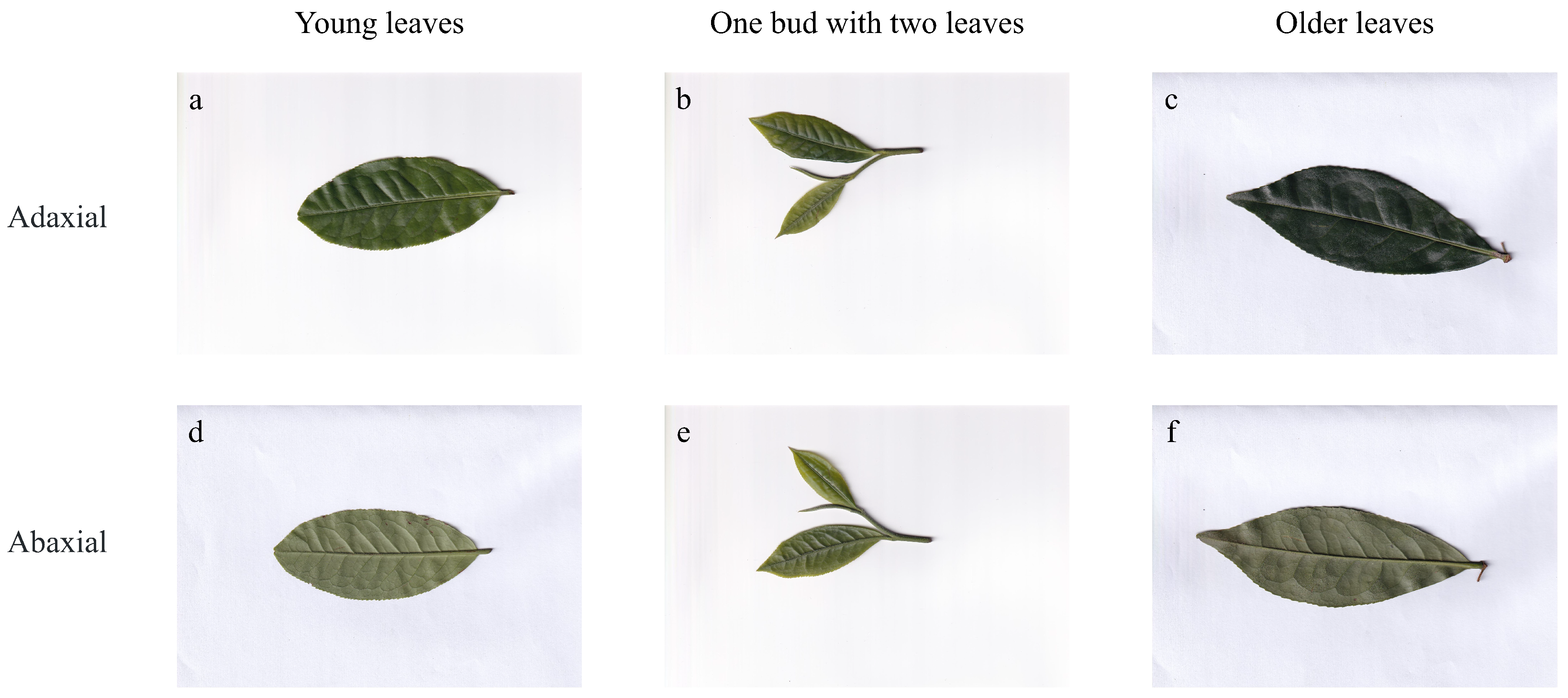
Figure 1.
Scanned images of tea leaves showing different views and developmental stages: (a) Adaxial view of young leaves, (b) Adaxial view of one bud with two leaves, (c) Adaxial view of older leaves, (d) Abaxial view of young leaves, (e) Abaxial view of one bud with two leaves, (f) Abaxial view of older leaves. This figure highlights the variations in appearance across different physiological ages and leaf surfaces.
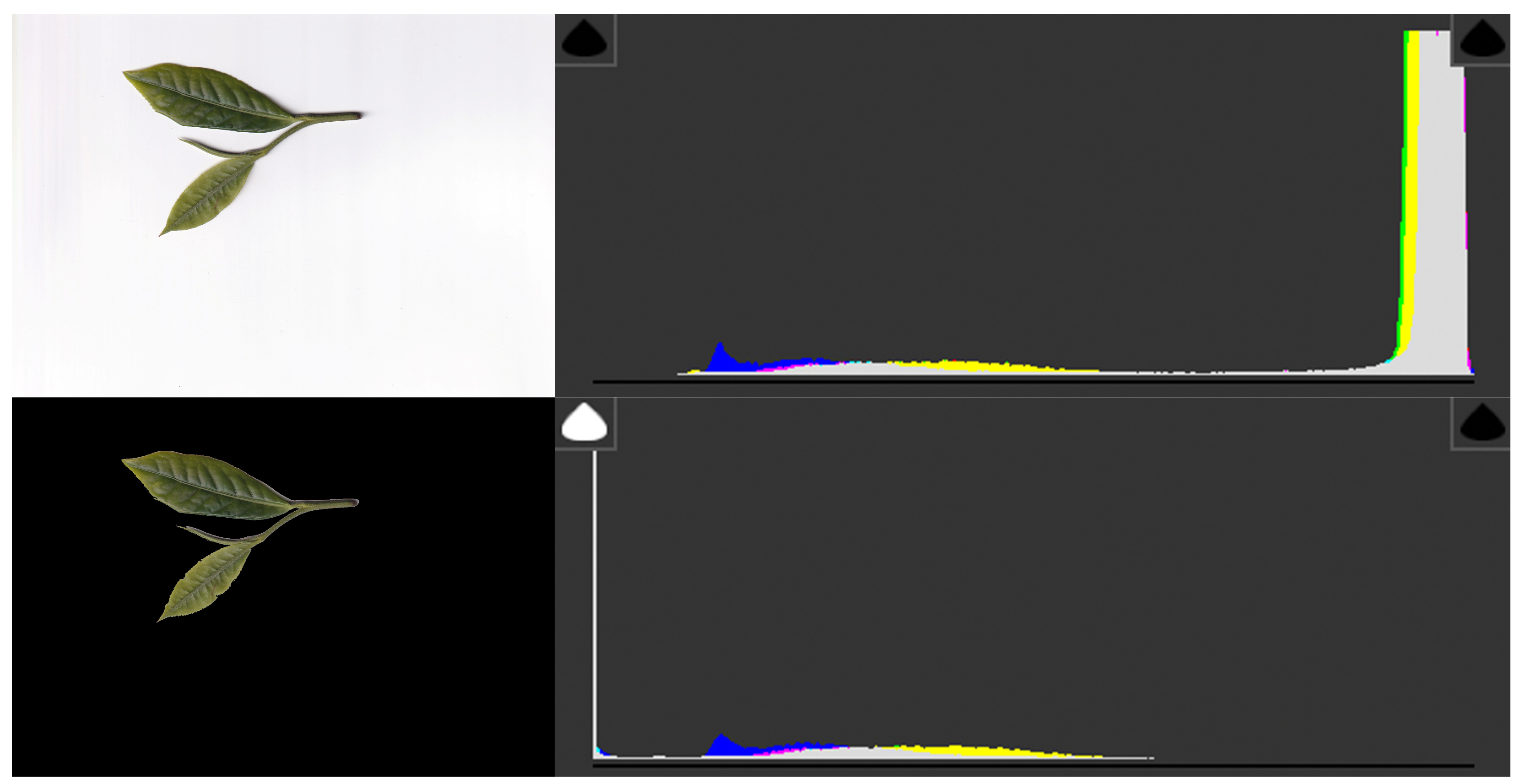
Figure 2.
Comparison of color/illumination histograms before and after background removal. (Top) Original scanned image of tea leaves with a white background and its RGB histograms, showing a strong peak in the high-intensity region due to the white background. (Bottom) Background-removed image with corresponding histograms, where the background peak disappears and the distributions more faithfully reflect leaf pixel values. This confirms that contour-based segmentation effectively reduces background-induced bias and preserves intra-class variation in leaf color and illumination.
Figure 3.
Portable chlorophyll and nitrogen analyzer (Model: HM-YC, Top Instrument Co., Ltd., Hangzhou, China) used for non-destructive measurement of leaf chlorophyll content. This instrument calculates the SPAD index based on light transmittance at 650 nm and 940 nm wavelengths, providing a rapid and reliable estimation of chlorophyll concentration and plant health.
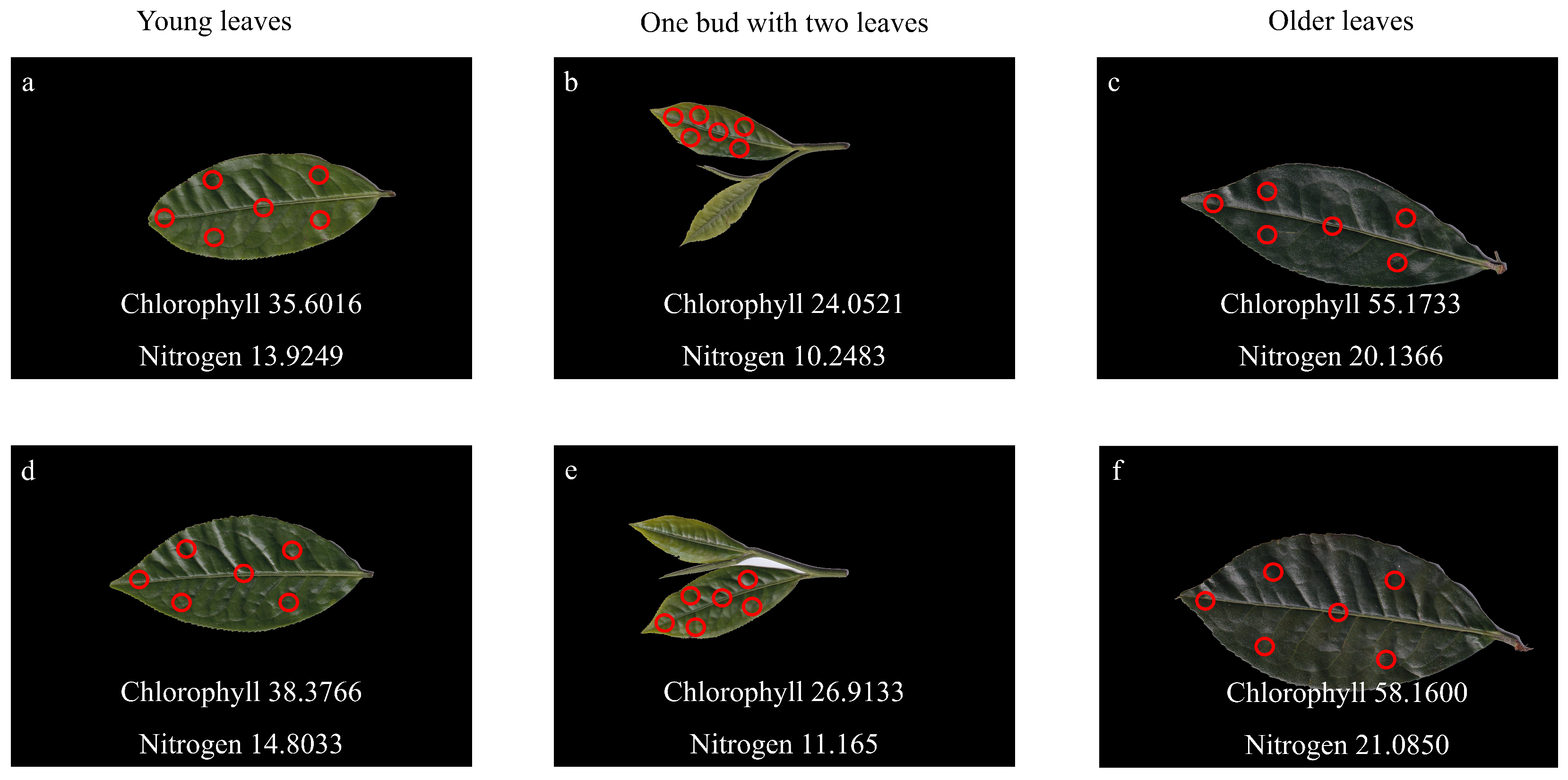
Figure 4.
Six-point sampling method for chlorophyll and nitrogen content measurement in tea leaves at different developmental stages. The upper row (a–c) shows the adaxial leaf surfaces, and the lower row (d–f) shows the abaxial surfaces. Red circles indicate the sampling regions used for chlorophyll and nitrogen measurement. (a,d) Young leaves; (b,e) One bud with two leaves; (c,f) Older leaves.
Figure 5.
The diagram presents the complete network structure from the input layer to the output layer, encompassing convolutional stages (S0 to S1) and attention stages (S2 to S4). Notably, it demonstrates how the integration of depthwise convolution with relative attention mechanisms effectively captures local features and global contextual information, thereby achieving robust processing capabilities across various data scales.
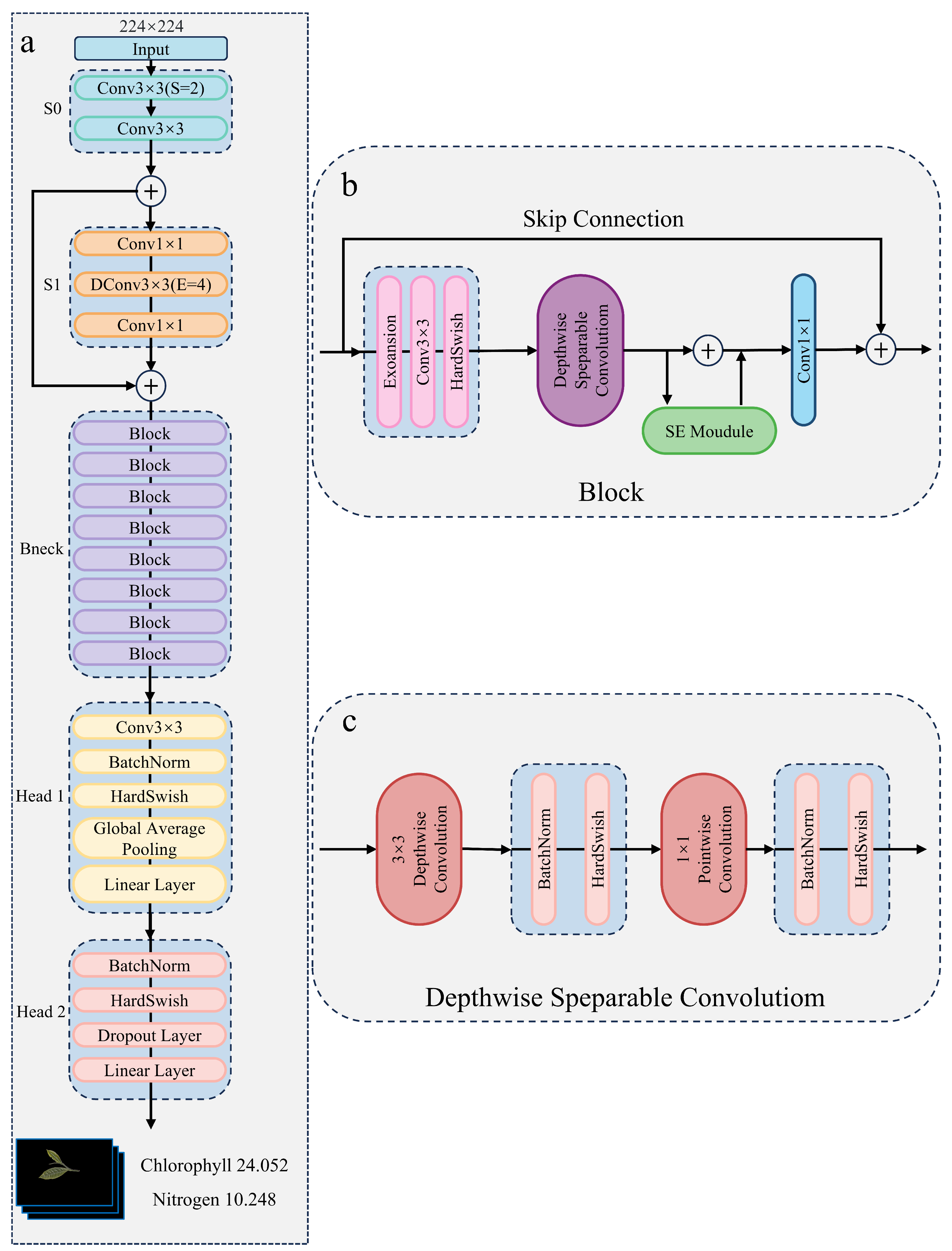
Figure 6.
(a) Overall structure of the improved CoAtNet-based model. (b) Internal design of the MobileNetV3-inspired Bneck block. (c) Structure of the depthwise separable convolution used in Bneck blocks.
Figure 6.
(a) Overall structure of the improved CoAtNet-based model. (b) Internal design of the MobileNetV3-inspired Bneck block. (c) Structure of the depthwise separable convolution used in Bneck blocks.
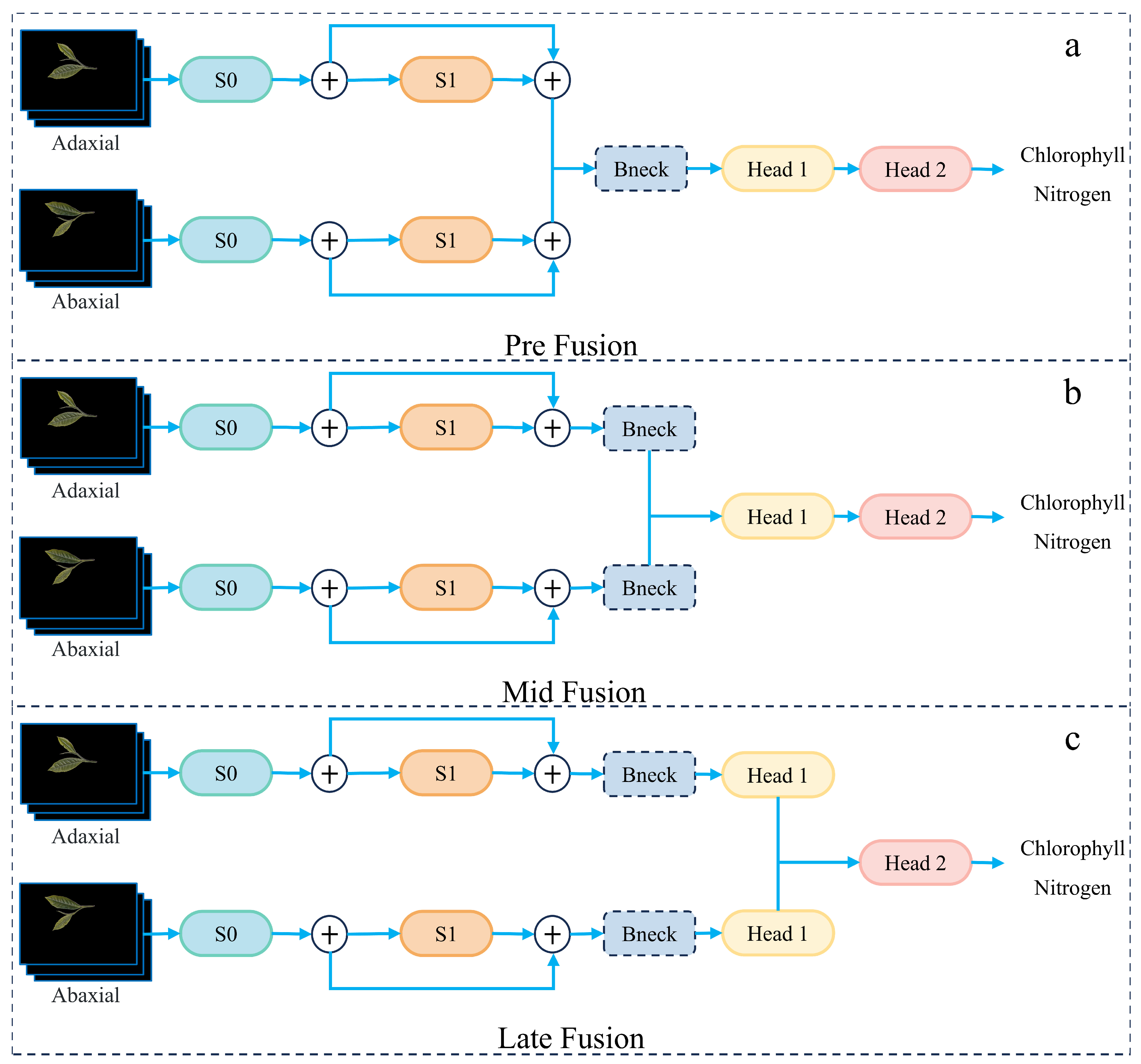
Figure 7.
Comparison of the three fusion strategies: (a) Pre-fusion after S1, (b) Mid-fusion after Bneck, and (c) Late-fusion after the prediction heads.
Figure 7.
Comparison of the three fusion strategies: (a) Pre-fusion after S1, (b) Mid-fusion after Bneck, and (c) Late-fusion after the prediction heads.
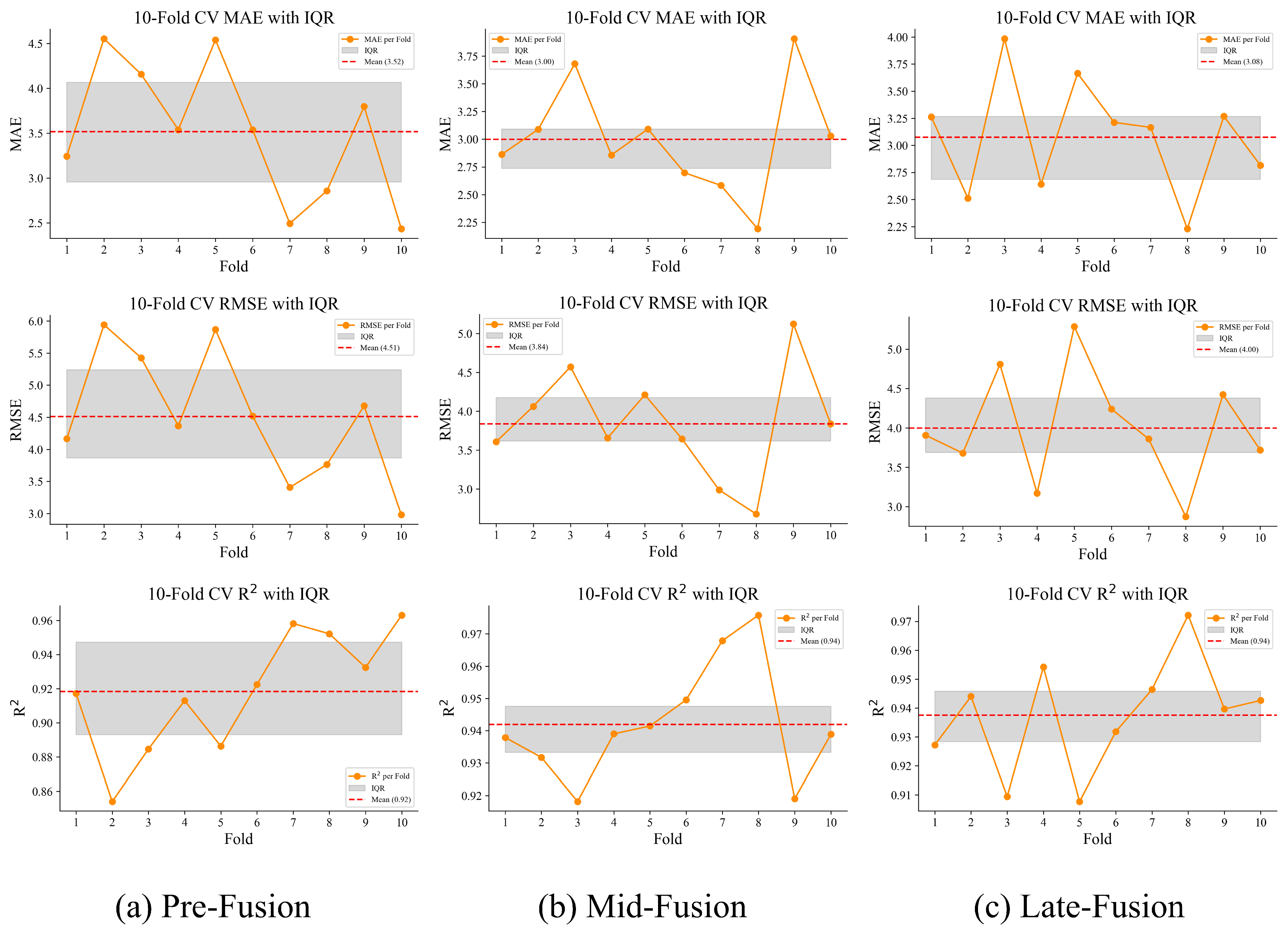
Figure 8.
Distribution of ten-fold cross-validation metrics (, , and ) for Pre-, Mid-, and Late-fusion strategies. The orange lines denote fold-wise metric values, the gray shaded areas represent the IQR, and the red dashed lines indicate mean values across folds. Mid-fusion demonstrates the narrowest IQR and the lowest error metrics, underscoring its stability and robustness.
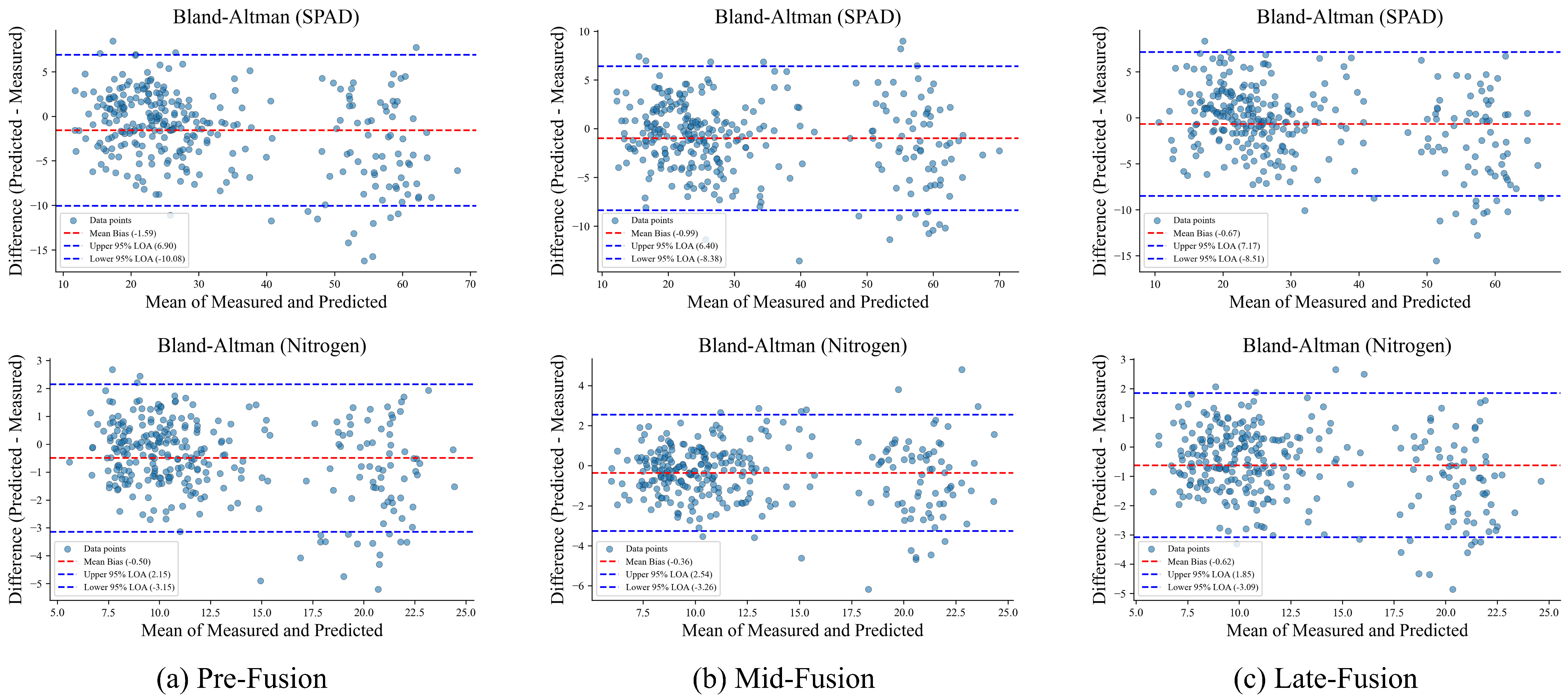
Figure 9.
Bland–Altman analysis of predicted versus measured values for SPAD and nitrogen content under different fusion strategies. The red dashed line denotes the mean bias, while the blue dashed lines mark the 95% LOA. Mid-fusion shows the smallest bias and narrowest LOA, confirming its superior predictive agreement.
Figure 10.
Ten-fold cross-validation per fold with IQR for adaxial, Mid-fusion, and abaxial inputs. The orange lines indicate per fold, gray shaded areas represent the IQR, and the red dashed lines denote the mean .
Figure 10.
Ten-fold cross-validation per fold with IQR for adaxial, Mid-fusion, and abaxial inputs. The orange lines indicate per fold, gray shaded areas represent the IQR, and the red dashed lines denote the mean .
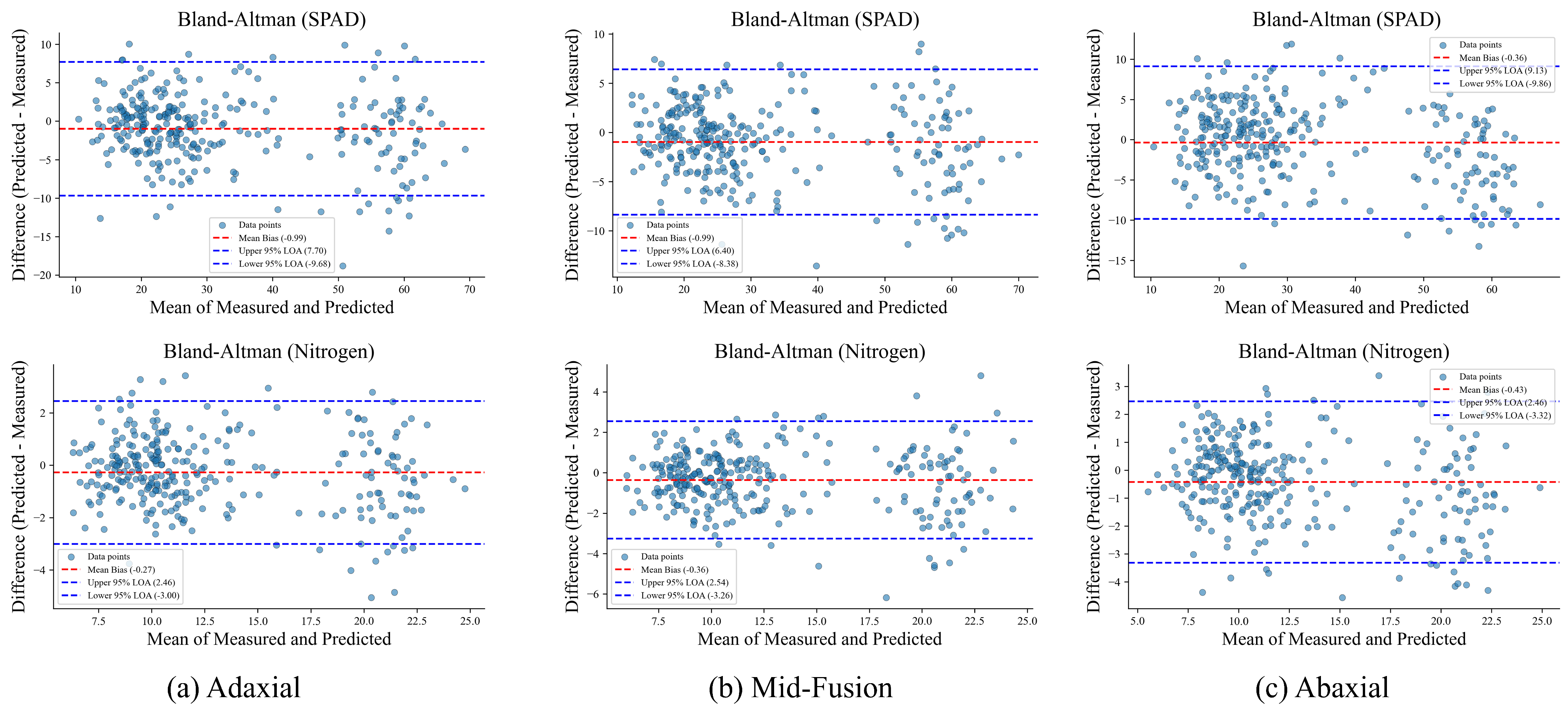
Figure 11.
Bland-Altman plots comparing predicted versus measured values for SPAD (top row) and nitrogen content (bottom row) under adaxial, Mid-fusion, and abaxial inputs. The red dashed lines denote mean bias, and the blue dashed lines represent 95% LOA.
Figure 11.
Bland-Altman plots comparing predicted versus measured values for SPAD (top row) and nitrogen content (bottom row) under adaxial, Mid-fusion, and abaxial inputs. The red dashed lines denote mean bias, and the blue dashed lines represent 95% LOA.
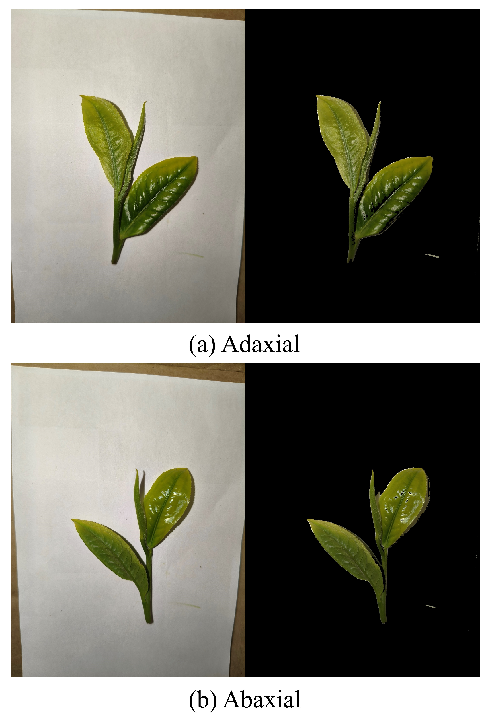
Figure 12.
Example of smartphone-acquired tea leaf images. A white paper was placed beneath the leaves to reduce background interference, and images were processed via contour-based background removal.
Figure 12.
Example of smartphone-acquired tea leaf images. A white paper was placed beneath the leaves to reduce background interference, and images were processed via contour-based background removal.
Figure 13.
Prediction results of the dual-view RGB model on the mixed-device test set. The red line represents the perfect fit (true values), while scatter points correspond to model predictions for SPAD and nitrogen contents.
Figure 13.
Prediction results of the dual-view RGB model on the mixed-device test set. The red line represents the perfect fit (true values), while scatter points correspond to model predictions for SPAD and nitrogen contents.
Table 1.
Distribution of tea leaf samples collected from four regions in Lincang, Yunnan Province, categorized by developmental stages.
Table 1.
Distribution of tea leaf samples collected from four regions in Lincang, Yunnan Province, categorized by developmental stages.
| Region | Young Leaves | One Bud with Two Leaves | Older Leaves | Total |
|---|
| Dele | 20 | 40 | 20 | 80 |
| Mangdan | 25 | 50 | 25 | 100 |
| Santa | 15 | 29 | 15 | 59 |
| Xiaomenglong | 15 | 30 | 15 | 60 |
| Total | 75 | 149 | 75 | 299 |
Table 2.
Feature map dimensions at key stages of Pre-fusion, Mid-fusion, and Late-fusion models.
Table 2.
Feature map dimensions at key stages of Pre-fusion, Mid-fusion, and Late-fusion models.
| Stage | Pre-Fusion | Mid-Fusion | Late-Fusion |
|---|
| Input | | | |
| S0 | | | |
| S1 | (after concat: ) | | |
| Bneck | | (after concat: ) | |
| Head 1 | | | (after concat: ) |
| Head 2 | | | |
Table 3.
Summary of experimental hyperparameters and settings.
Table 3.
Summary of experimental hyperparameters and settings.
| Parameter | Description |
|---|
| Batch size | 32 |
| Number of epochs | 100 |
| Initial learning rate | 0.0005 |
| Optimizer | AdamW |
| Loss function | Mean Squared Error (MSE) |
| Cross-validation | ten-fold |
| Fusion strategies | Pre-fusion, Mid-fusion, Late-fusion |
Table 4.
Ten-fold cross-validation results of the Pre-fusion strategy.
Table 4.
Ten-fold cross-validation results of the Pre-fusion strategy.
| Fold | | | (%) |
|---|
| 1 | 4.16 | 3.24 | 91.72 |
| 2 | 5.94 | 4.55 | 85.39 |
| 3 | 5.43 | 4.16 | 88.46 |
| 4 | 4.37 | 3.54 | 91.30 |
| 5 | 5.87 | 4.54 | 88.63 |
| 6 | 4.52 | 3.54 | 92.25 |
| 7 | 3.41 | 2.49 | 95.82 |
| 8 | 3.76 | 2.86 | 95.22 |
| 9 | 4.68 | 3.80 | 93.25 |
| 10 | 2.98 | 2.43 | 96.32 |
| Mean ± Std | 4.51 ± 0.86 | 3.52 ± 0.60 | 91.84 ± 3.58 |
Table 5.
Ten-fold cross-validation results of the Mid-fusion strategy.
Table 5.
Ten-fold cross-validation results of the Mid-fusion strategy.
| Fold | | | (%) |
|---|
| 1 | 3.61 | 2.86 | 93.79 |
| 2 | 4.06 | 3.09 | 93.17 |
| 3 | 4.57 | 3.68 | 91.81 |
| 4 | 3.66 | 2.86 | 93.90 |
| 5 | 4.21 | 3.09 | 94.14 |
| 6 | 3.64 | 2.70 | 94.96 |
| 7 | 2.99 | 2.58 | 96.79 |
| 8 | 2.68 | 2.19 | 97.58 |
| 9 | 5.12 | 3.91 | 91.90 |
| 10 | 3.84 | 3.03 | 93.89 |
| Mean ± Std | 3.84 ± 0.65 | 3.00 ± 0.45 | 94.19 ± 1.75 |
Table 6.
Ten-fold cross-validation results of the Late-fusion strategy.
Table 6.
Ten-fold cross-validation results of the Late-fusion strategy.
| Fold | | | (%) |
|---|
| 1 | 3.91 | 3.26 | 92.72 |
| 2 | 3.68 | 2.51 | 94.40 |
| 3 | 4.81 | 3.98 | 90.94 |
| 4 | 3.17 | 2.64 | 95.42 |
| 5 | 5.29 | 3.66 | 90.77 |
| 6 | 4.24 | 3.21 | 93.18 |
| 7 | 3.86 | 3.17 | 94.64 |
| 8 | 2.87 | 2.23 | 97.21 |
| 9 | 4.42 | 3.27 | 93.96 |
| 10 | 3.72 | 2.82 | 94.26 |
| Mean ± Std | 4.00 ± 0.64 | 3.08 ± 0.52 | 93.75 ± 1.88 |
Table 7.
Performance comparison of different fusion strategies.
Table 7.
Performance comparison of different fusion strategies.
| Strategy | | | (%) | Parameters (M) |
|---|
| Pre-fusion | 4.51 ± 0.86 | 3.52 ± 0.60 | 91.84 ± 3.58 | 1.88 |
| Mid-fusion | 3.84 ± 0.65 | 3.00 ± 0.45 | 94.19 ± 1.75 | 1.92 |
| Late-fusion | 4.00 ± 0.64 | 3.08 ± 0.52 | 93.75 ± 1.88 | 2.60 |
Table 8.
Ten-fold cross-validation results using only adaxial images.
Table 8.
Ten-fold cross-validation results using only adaxial images.
| Fold | | | (%) |
|---|
| 1 | 4.77 | 3.89 | 89.16 |
| 2 | 5.06 | 3.97 | 89.40 |
| 3 | 6.63 | 4.83 | 82.79 |
| 4 | 3.20 | 2.54 | 95.32 |
| 5 | 4.36 | 3.12 | 93.71 |
| 6 | 3.91 | 3.24 | 94.21 |
| 7 | 4.81 | 3.90 | 91.69 |
| 8 | 3.05 | 2.32 | 96.85 |
| 9 | 4.88 | 3.40 | 92.65 |
| 10 | 3.61 | 2.68 | 94.60 |
| Mean ± Std | 4.43 ± 0.96 | 3.39 ± 0.72 | 92.04 ± 3.88 |
Table 9.
Ten-fold cross-validation results using only abaxial images.
Table 9.
Ten-fold cross-validation results using only abaxial images.
| Fold | | | (%) |
|---|
| 1 | 4.72 | 3.85 | 89.36 |
| 2 | 3.29 | 2.52 | 95.52 |
| 3 | 6.45 | 5.34 | 83.68 |
| 4 | 4.32 | 3.39 | 91.49 |
| 5 | 4.83 | 3.88 | 92.29 |
| 6 | 5.51 | 4.59 | 88.47 |
| 7 | 4.70 | 4.00 | 92.05 |
| 8 | 4.16 | 3.13 | 94.15 |
| 9 | 4.94 | 3.99 | 92.46 |
| 10 | 5.00 | 4.26 | 89.62 |
| Mean ± Std | 4.79 ± 0.83 | 3.89 ± 0.78 | 90.91 ± 3.78 |
Table 10.
Comparison of prediction performance under different input configurations.
Table 10.
Comparison of prediction performance under different input configurations.
| Input Setting | | | (%) |
|---|
| Adaxial Only | 4.43 ± 0.96 | 3.39 ± 0.72 | 92.04 ± 3.88 |
| Abaxial Only | 4.79 ± 0.83 | 3.89 ± 0.78 | 90.91 ± 3.78 |
| Dual-View | 3.84 ± 0.65 | 3.00 ± 0.45 | 94.19 ± 1.75 |
Table 11.
Ten-fold cross-validation results of the baseline CoAtNet with Dual-View.
Table 11.
Ten-fold cross-validation results of the baseline CoAtNet with Dual-View.
| Fold | | | (%) |
|---|
| 1 | 4.03 | 3.27 | 92.27 |
| 2 | 5.46 | 3.99 | 87.67 |
| 3 | 4.04 | 3.14 | 93.60 |
| 4 | 4.91 | 3.46 | 89.01 |
| 5 | 6.27 | 5.12 | 87.03 |
| 6 | 4.27 | 3.53 | 93.06 |
| 7 | 3.73 | 2.91 | 94.98 |
| 8 | 3.72 | 3.09 | 95.32 |
| 9 | 4.78 | 3.97 | 92.96 |
| 10 | 3.83 | 3.05 | 93.92 |
| Mean ± Std | 4.50 ± 0.77 | 3.55 ± 0.57 | 91.98 ± 2.74 |
Table 12.
Comparison between the baseline CoAtNet and our model.
Table 12.
Comparison between the baseline CoAtNet and our model.
| Model | | | (%) | Parameters (M) |
|---|
| CoAtNet | 4.50 ± 0.77 | 3.55 ± 0.57 | 91.98 ± 2.74 | 17.02 |
| Our model | 3.84 ± 0.65 | 3.00 ± 0.45 | 94.19 ± 1.75 | 1.92 |
Table 13.
Performance comparison of different models under adaxial, abaxial, and dual-view configurations.
Table 13.
Performance comparison of different models under adaxial, abaxial, and dual-view configurations.
| Model | | | (%) | Parameters (M) |
|---|
| Abaxial |
| ResMLP | 6.91 ± 1.16 | 5.43 ± 0.84 | 81.12 ± 7.21 | 15.35 |
| MobileNetV3 | 7.82 ± 2.37 | 6.23 ± 2.02 | 73.76 ± 18.54 | 1.68 |
| TinyViT | 4.59 ± 0.59 | 3.71 ± 0.54 | 91.74 ± 2.40 | 5.07 |
| StartNet | 6.81 ± 1.98 | 5.88 ± 2.02 | 80.16 ± 13.41 | 2.68 |
| GhostNet | 7.38 ± 3.27 | 5.80 ± 2.76 | 76.03 ± 22.13 | 6.86 |
| ResNet34 | 6.04 ± 4.46 | 5.05 ± 4.13 | 80.82 ± 32.50 | 21.29 |
| CoAtNet | 5.39 ± 1.24 | 4.16 ± 0.99 | 88.22 ± 4.82 | 17.03 |
| KNN | 7.811 ± 1.140 | 5.969 ± 0.768 | 76.1 ± 4.1 | - |
| MLR | 8.896 ± 1.540 | 6.635 ± 1.027 | 68.0 ± 9.6 | - |
| SVR | 10.032 ± 2.054 | 7.491 ± 1.489 | 59.4 ± 13.7 | - |
| Ours | 4.79 ± 0.83 | 3.89 ± 0.78 | 90.91 ± 3.78 | 2.79 |
| Adaxial |
| ResMLP | 5.35 ± 0.92 | 4.15 ± 0.71 | 88.61 ± 4.57 | 15.35 |
| MobileNetV3 | 9.28 ± 5.86 | 7.35 ± 5.08 | 58.12 ± 53.33 | 1.68 |
| TinyViT | 4.50 ± 0.56 | 3.54 ± 0.54 | 91.91 ± 3.02 | 5.07 |
| StartNet | 6.42 ± 2.15 | 5.54 ± 2.02 | 82.75 ± 11.46 | 2.68 |
| GhostNet | 8.78 ± 3.12 | 7.34 ± 2.98 | 66.58 ± 22.96 | 6.86 |
| ResNet34 | 6.01 ± 5.73 | 4.99 ± 5.28 | 74.31 ± 57.81 | 21.29 |
| CoAtNet | 4.20 ± 0.71 | 3.12 ± 0.43 | 93.03 ± 2.55 | 17.03 |
| KNN | 8.458 ± 0.850 | 6.495 ± 0.912 | 71.2 ± 6.7 | - |
| MLR | 6.408 ± 1.229 | 4.821 ± 0.973 | 82.9 ± 7.1 | - |
| SVR | 9.875 ± 1.215 | 7.403 ± 1.079 | 60.4 ± 11.1 | - |
| Ours | 4.43 ± 0.96 | 3.39 ± 0.72 | 92.04 ± 3.88 | 2.79 |
| Fusion/Dual-View |
| ResMLP | 6.60 ± 1.67 | 5.04 ± 1.08 | 81.64 ± 11.87 | 15.26 |
| MobileNetV3 | 6.47 ± 1.88 | 5.01 ± 1.26 | 82.10 ± 12.60 | 2.41 |
| TinyViT | 4.55 ± 0.71 | 3.54 ± 0.50 | 91.72 ± 2.13 | 5.73 |
| StartNet | 6.81 ± 1.98 | 5.88 ± 2.02 | 80.16 ± 13.41 | 2.68 |
| GhostNet | 5.94 ± 1.21 | 4.85 ± 1.16 | 85.70 ± 6.75 | 3.16 |
| ResNet34 | 6.04 ± 4.46 | 5.05 ± 4.13 | 80.82 ± 32.50 | 21.29 |
| CoAtNet | 4.50 ± 0.84 | 3.55 ± 0.66 | 91.98 ± 2.99 | 17.02 |
| KNN | 8.118 ± 1.509 | 6.225 ± 1.094 | 73.2 ± 9.1 | - |
| MLR | 6.916 ± 0.842 | 5.184 ± 0.576 | 80.8 ± 4.3 | - |
| SVR | 9.988 ± 1.557 | 7.628 ± 1.315 | 59.7 ± 12.0 | - |
| Ours | 3.84 ± 0.65 | 3.00 ± 0.45 | 94.19 ± 1.75 | 1.92 |
Table 14.
Representative studies on leaf trait prediction with single- or dual-view inputs and different imaging modalities. , , and values are provided to situate the performance of the proposed dual-view Mid-fusion model.
Table 14.
Representative studies on leaf trait prediction with single- or dual-view inputs and different imaging modalities. , , and values are provided to situate the performance of the proposed dual-view Mid-fusion model.
| Study | Modality | | | (%) |
|---|
| Tang et al., 2023 [39] | RGB single-view (microalgae) | 2.36 | - | 66.00 |
| Zhang et al., 2023 [41] | Hyperspectral UAV (Chinese cabbage) | - | - | 71.0 |
| Hu et al., 2024 [42] | Hyperspectral (rice N content) | 0.08 | 3.89 | - |
| Azadnia et al., 2023 [40] | Vis/NIR spectroscopy (apple) | 0.01 | - | 97.80 |
| Barman and Choudhury, 2022 [43] | Smartphone RGB (citrus) | 0.26 | 0.07 | 94.00 |
| Ours | RGB dual-view (tea) | 3.84 | 3.00 | 94.19 |
