Are Supervised Learning Methods Suitable for Estimating Crop Water Consumption under Optimal and Deficit Irrigation?

Abstract

This study examined the performance of random forest (RF), support vector machine (SVM) and adaptive boosting (AB) machine learning models used to estimate daily potato crop evapotranspiration adjusted (ET_c-adj) under full irrigation (I₁₀₀), 50% of full irrigation supply (I₅₀) and rainfed cultivation (I₀). Five scenarios of weather, crop and soil data availability were considered: (S1) reference evapotranspiration and precipitation, (S2) S1 and crop coefficient, (S3) S2, the fraction of total available water and root depth, (S4) S2 and total soil available water, and (S5) S3 and total soil available water. The performance of machine learning models was compared with the standard FAO56 calculation procedure. The most accurate ET_c-adj estimates were observed with AB4 for I₁₀₀, RF3 for I₅₀ and AB5 for I₀ with coefficients of determination (R²) of 0.992, 0.816 and 0.922, slopes of 1.004, 0.999 and 0.972, modelling efficiencies (EF) of 0.992, 0.815 and 0.917, mean absolute errors (MAE) of 0.125, 0.405 and 0.241 mm day⁻¹, root mean square errors (RMSE) of 0.171, 0.579 and 0.359 mm day⁻¹ and mean squared errors (MSE) of 0.029, 0.335 and 0.129 mm day⁻¹, respectively. The AB model is suggested for ET_c-adj prediction under I₁₀₀ and I₀ conditions, while the RF model is recommended under the I₅₀ condition.

1. Introduction

Crop growth and production are influenced by agro-meteorological, soil and crop variables as well as agronomic practices related to water/nutrient supply and pesticide/herbicide applications. Specific attention is given to the availability of water since it is a limited resource in many arid and semi-arid regions, like the Mediterranean [1]. In these regions, nonoptimal irrigation is a common cultivation practice and water stress occurs frequently as a main abiotic factor that limits crop growth and yield [2,3]. Therefore, the evaluation of water stress and efficient water management is of crucial importance for agricultural production, especially in areas suffering from water scarcity.

In the last few decades, coping with water scarcity has become particularly complex due to climate change and the variability of weather conditions [4,5]. The impact of climate change on Mediterranean agriculture is already evident in many areas, especially in arid and semi-arid regions [6]. Several studies reported evidence of climate change in the last few decades over the Mediterranean and tried to foresee the expected trend and its impact on Mediterranean agriculture in the future [1,7,8,9]. Frequent droughts, flash floods, heat spells and spring frosts triggered a decline in agricultural production, further depletion of water resources, soil erosion and impoverishment, land abandonment and desertification and have increased pressures on food security and socio-economic development, particularly in marginal rural zones [10].

Numerous studies have been conducted on the impact of climate change on crop abiotic stresses and production at different scales [2,11,12,13]. Some authors [11,13,14] applied crop growth models to simulate crop growth dynamics and forecast agricultural production under climate change conditions. A common conclusion is that warm and dry climates adversely affect crop phenology and yield. Hence, the challenge is to optimise the use of resources (water and nutrients) while increasing yields and reducing environmental impacts [1,12]. In this context, the application of deficit irrigation [12,15], mulching [16,17] and the use of bio-stimulants [18,19,20,21,22] and other water-saving practices have become frequent with the aim of attenuating the negative impact of abiotic stresses, positively affecting plant physiological processes [19,20,21] and improving soil health [22].

The adoption of a precision agriculture approach based on the continuous monitoring of weather and hydrological variables, water, nutrients and carbon balance represents the preconditions and priorities for interventions and research. Equally, proactive management tools (e.g., early warning systems and water/nutrient management decision support systems considering remote sensing and weather forecasting data) and on-ground measurements are of primary importance to attenuate the negative impacts of extreme weather events and various abiotic stresses [1,4,12,23]. The success of such measures is based on the interactive use of certified, innovative technological solutions (i.e., the new generation of sensors, unmanned aerial vehicles, artificial intelligence, the Internet of Things and cloud-based applications) and the adoption of site-specific and resource-optimised management practices and varieties able to respond to adverse environmental conditions and to increase/stabilise yields and water productivity [2,4].

Potato (Solunum tuberosum L.) is a common Solanaceous crop. Moreover, it is one of the largest cultivated food crops in the world and has an important nutritional value [15]. Globally, potato production is about 388.2 million Mg of fresh yield from about 19.3 million ha [24]. In the Mediterranean region, it is cultivated on more than 1 million ha, with a production of about 32 million Mg of tubers [25].

Irrigation is necessary to meet crop water requirements due to erratic and insufficient rainfall for most potato-cultivated areas [26]. When water availability is limited and evapotranspiration demand is high, potato yield is negatively affected, even if briefly exposed to water stress because of its shallow root system [27,28,29]. Therefore, it is important to adopt the best water management solutions as a function of overall water availability, weather and soil data and the crop response to water stress during the entire growing season. An optimal water supply is particularly relevant during tuber development and bulking since these stages are predominantly affected by water stress [30,31]. For the rest of the growing season, regulated deficit irrigation strategies might be a solution [15,25,32]. Hence, the estimation of daily crop evapotranspiration adjusted for water stress (ETc-adj) is of vital importance in water-limited agricultural areas. The knowledge of ETc-adj on a daily basis gives an idea of the effective water uptake from the root zone, which supports the optimisation of irrigation scheduling and the enhancement of crop water productivity.

Hydrology and environmental studies, including agriculture, are characterised by complex processes which include many interactions. For example, crop evapotranspiration (ETc) is influenced by atmospheric and soil conditions, plant/canopy characteristics and applied agronomic measures (irrigation water quantity and quality, the supply of nutrients, plant diseases, pests and weeds management, etc.) [33,34]. Today, these interactions can be successfully described by modern mathematical tools, including the application of machine learning methods. In the last few years, various machine learning methods have been tested to estimate both reference and crop ET [35,36,37,38,39,40,41,42,43,44]. In particular, these methods have been developed to enhance the prediction accuracy for the estimation of ETo with limited data availability and ETc under optimal water supply. For example, Yamaç [45] examined adaptive boosting (AB), k-nearest neighbour (kNN), random forest (RF) and support vector machine (SVM) methods for modelling sugar beet ETc in Türkiye. The models, considering eight scenarios of climate input data demonstrated their applicability for sugar beet ETc estimation. Saggi and Jain [46] studied regularisation random forest (RRF) and the fuzzy-genetic (FG) models for estimating maize and wheat ETc in India. They found that the proposed FG and RRF models are suitable for maize and wheat ETc prediction. Chen et al. [47] investigated temporal convolution network (TCN) models comprising long short-term memory networks (LSTM) and deep neural networks (DNN) for modelling maize ETc under mulched drip irrigation. They highlighted that the TCN models performed well in predicting maize ETc under mulched drip irrigation in China. Feng et al. [48] analysed the reliability of extreme learning machine (ELM) and generalised regression neural network (GRNN) for maize ETc estimation in China. The models confirmed better performance using meteorological and crop data as input variables. Aghajanloo et al. [49] applied artificial neural network (ANN), GANN and multivariate nonlinear regression (MNLR) models to predict potato ETc in Iran. The results indicated that all the models used could estimate ETc with the intended level of accuracy. While the aforementioned studies demonstrated the applicability of different machine learning methods to estimate ETc under optimal water supply, there is a lack of studies addressing the estimate of crop evapotranspiration adjusted for water stress (ETc-adj) using machine learning techniques. The present study aims to fill this gap.

Crop evapotranspiration under optimal and water stress conditions is commonly computed using the methodology proposed by the FAO Irrigation and Drainage Paper 56 [33], which considers the impact of weather through reference evapotranspiration (ETo), crop characteristics through crop coefficient (Kc) and the water stress level through water stress coefficient (Ks). ETo is estimated using the Penman–Monteith (PM) equation as suggested by the FAO [33]. This method is physically based and has demonstrated its superiority when compared to other empirical methods and equations [34,50,51,52]. The crop coefficient (Kc) is a variable that encompasses numerous crop characteristics, including crop type and variety, crop growth stage, crop density and height, percentage of ground cover, etc. [33,34]. Nevertheless, water stress coefficient (Ks) depends not only on crop sensitivity to water stress but also on soil characteristics, including texture (soil water holding capacity) and effective management depth, which is linked to the rooting system growth. Therefore, estimation of crop evapotranspiration requires knowledge and interaction of weather, crop and soil data and their variability during the crop growing season. In most cases, only some of the above data are available, which affects the estimation of crop ET, especially under water stress.

The aim of the present study was to examine the performance metric of machine learning methods (RF, SVM and AB) for the prediction of potato ETc under both optimal and limited water supply conditions, corresponding to full irrigation (I₁₀₀), deficit irrigation with 50% of I100 (I₅₀) and rainfed cultivation (I₀). Five scenarios of available weather, crop and soil input data were considered. The study aimed to determine the best performance metric for each specific input data scenario for estimation of potato evapotranspiration under optimal conditions (ETc) and under deficit water supply (ETc_adj). Thus, unlike the previous study [53], which focused on optimal water supply, this study focuses on predicting ETc under water stress and various scenarios using weather, soil and crop data. To the best of the authors’ knowledge, this is one of the first studies to evaluate machine learning methods for prediction of ETc_adj, i.e., crop evapotranspiration under water stress, across different data availability scenarios.

2. Materials and Methods

2.1. Study Area and Experiment Design

The data were collected from field experiments conducted in 2009 and 2010 at the Mediterranean Agronomic Institute of Bari (CIHEAM-Bari), located in Valenzano, Southern Italy (41°03′16″ N, 16°52′ E, 72 m altitude) (Figure 1). According to the Köpper–Geiger classification [54], the research area has a Mediterranean climate. The average annual precipitation over 30 years is approximately 550 mm, mainly concentrated in autumn and winter seasons. An automatic agro-meteorological station collected daily meteorological data near the field trail site. The dataset included maximum and minimum air temperature (T_max and T_min), solar radiation (R_n), maximum and minimum air relative humidity (RH_max and RH_min), wind speed at 2 m height (U₂) and precipitation (P).

Potato cv Spunta was cultivated over two growing seasons. This cultivar is highly preferred by farmers in the Mediterranean region due to its tolerance to water stress and its potential for high yield [55]. The potatoes were planted at a density of 5 plants m⁻², with rows spaced 0.8 m apart and plants 0.25 m apart within rows. The soil, classified as shallow (0.5–0.6 m depth) with a silty loam texture following the USDA particle-size classification (USDA, 2006), had a maximum root depth that was fixed at 0.5 m. The experimental season commenced two weeks earlier in 2010 (3 March) compared to 2009 (17 March).

The crop was grown under three water regimes: (i) optimal irrigation (I₁₀₀), aimed at meeting the crop’s water requirements optimally, (ii) deficit irrigation (I₅₀), supplying 50% of the crop’s water requirements, and (iii) rainfed cultivation (I₀). The treatments were arranged in a split plot design with three replicates. Each plot measured 7 m by 7 m in the experiment.

An Excel-based tool version 8.0 [56], employing the standard FAO 56 methodology [33], was utilised for irrigation scheduling. The tool utilises weather, soil and crop data to estimate ETc and employs a simple water balance model to determine soil water content in the effective root zone on a daily basis. The soil gravimetric method was used to periodically adjust soil water content in the root zone and to monitor and potentially adjust the soil water content estimated by the model [57]. For optimal irrigation treatment, localised drip irrigation was employed to maintain soil water content within the predefined optimum yield threshold of 40% related to the total available water content in the root zone. The net irrigation supply was 330 and 237 mm in 2009 and 2010, respectively. Deficit irrigation was scheduled on the same dates as optimal irrigation but with irrigation amounts two times lower. Further details about the field experiment are available in Cantore et al. [25].

2.2. Weather, Crop and Soil Data

A synthesis of average weather data for both years is presented in

Table 1. Average weather parameters describing the crop growing seasons of 2009 and 2010 (T: air temperature, Rn: solar radiation, RH: air relative humidity, U₂: wind speed at 2 m height, P: precipitation).

	T	Rn	RH	U2	P
	°C	MJ m−2	%	m s−1	Mm
Year
2009	18.4	23.0	65.8	0.9	272.2
2010	16.2	19.8	67.5	1.2	170.8

. The growing season of 2009 experienced greater precipitation (for 101.4 mm) and higher air temperatures (for 2.2 °C) compared to 2010. Additionally, in 2009, solar radiation was higher by 3.2 MJ m⁻² than in 2010, while relative humidity and windspeed were lower in 2009 than in 2010. The variation in weather variables is primarily attributed to the earlier start of the growing season in 2010 compared to 2009.

The crop growing stages were divided into four periods: initial, crop development, mid-season and late season. The starting date and duration of each crop growth stage are provided in

Table 2. The length of potato crop growth stages during the 2 years of experiment.

	2009	Lenght of Growth Stages (Day)	2010	Lenght of Growth Stages (Day)
Crop growth stages
Initial	17 March–10 April	24	3 March–26 March	24
Crop development	11 April–17 May	37	27 March–11 May	45
Mid-season	18 May–13 June	27	12 May–8 June	28
Late season	14 June–10 July	27	9 June–23 June	15

. In 2009, the potato growing period was 3 days longer than in 2010 (115 vs. 112 days).

The crop coefficient (Kc) combines the effects of soil evaporation and crop transpiration during the crop growing season. The initial Kc was set to 0.5 according to the FAO 56 [33]. The mid-season crop coefficient (Kc_mid) and the end-season crop coefficient (Kcend) were adjusted based on the potato height (h), the average value of minimum relative humidity (RH_min) and wind speed measured at a height 2 m (U₂). The maximum crop height was 0.66 m during both growing periods. Consequently, the adjusted values of Kcmid and Kcend were 1.14 and 0.72 for 2009 and 1.11 and 0.76 for 2010, respectively [53].

The soil in the experimental field had a silty loam texture. Field capacity and wilting point were measured at 0.28 m³ m⁻³ and 0.13 m³ m⁻³, respectively. The allowed soil moisture depletion fraction for optimal irrigation (p) was set at 0.40, slightly higher than the value (0.35) proposed in FAO 56, reflecting the increased resistance to water stress of the potato variety (Spunta) compared to common potato varieties [25].

2.3. Estimation of Soil Water Balance and Adjusted Crop Evapotranspiration

A standard procedure recommended by FAO 56 [33] was followed for the estimation of crop evapotranspiration and soil water balance modelling. The main calculation steps are described below.

Reference evapotranspiration (ETo) in mm day⁻¹ was calculated using the Penman–Monteith (PM) equation. Under optimal water supply, crop evapotranspiration (ETc) was estimated by multiplying ETo by the crop coefficient (Kc). When the soil moisture depletion in the root zone (D_r) exceeded the optimum yield threshold (p), the ETc was adjusted to water stress (ETc_adj) and estimated using Equation (1):

$$\mathrm{E}\mathrm{T}\mathrm{c}\text{\_}\mathrm{a}\mathrm{d}\mathrm{j}=\mathrm{K}\mathrm{s} \mathrm{K}\mathrm{c} \mathrm{E}\mathrm{T}\mathrm{o}$$

(1)

The water stress coefficient (K_s) was computed as:

$$\mathrm{K}\mathrm{s}=\frac{\mathrm{T}\mathrm{A}\mathrm{W}-{\mathrm{D}}_{\mathrm{r}}}{\mathrm{T}\mathrm{A}\mathrm{W}-\mathrm{R}\mathrm{A}\mathrm{W}}=\frac{\mathrm{T}\mathrm{A}\mathrm{W}-{\mathrm{D}}_{\mathrm{r}}}{\left(1-\mathrm{p}\right)\mathrm{T}\mathrm{A}\mathrm{W}}\hspace{1em}\mathrm{f}\mathrm{o}\mathrm{r} {\mathrm{D}}_{\mathrm{r}}>\mathrm{R}\mathrm{A}\mathrm{W}$$

(2)

where p is the depletion fraction for no stress (0.4), TAW and RAW are, respectively, the total and readily available soil water (mm) relative to the rooting depth Zr, and RAW = p TAW. When D_r ≤ RAW, there is no water stress, Ks is equal to 1, and ETc_adj is equal to ETc. When D_r > RAW, water stress occurs and ETc_adj, estimated by Equation (1), is lower than ETc.

The soil water balance in the root zone was estimated as:

$${\mathrm{D}}_{\mathrm{r},\mathrm{i}}={\mathrm{D}}_{\mathrm{r},\mathrm{i}-1}-{\left(\mathrm{P}-\mathrm{R}\mathrm{O}\right)}_{\mathrm{i}}-{\mathrm{I}}_{\mathrm{i}}-{\mathrm{C}\mathrm{R}}_{\mathrm{i}}+{\mathrm{E}\mathrm{T}}_{\mathrm{c} \mathrm{a}\mathrm{d}\mathrm{j}}+{\mathrm{D}\mathrm{P}}_{\mathrm{i}}$$

(3)

where D_r,i is root zone depletion at the end of day _i, D_r,i−1 represents the root zone depletion at the end of previous day (I − 1), P_i denotes effective precipitation, RO_i stands for surface runoff, I_i indicates net irrigation depth, Cri accounts for capillary rise, ETc adj represents crop ET calculated by Equation (4) and DP_i signifies deep percolation. All variables are measured in mm and subscript _i corresponds to a specific day. In the study area, the water table was exceptionally deep and the field was flat with proper land management. Consequently, the impacts of CR and RO were disregarded. DP was estimated using the method proposed by Liu et al. [58].

2.4. Machine Learning Methods

2.4.1. Random Forest

The random forest (RF) method was initially introduced by Breiman [59] for forecasting problems. The working phases of the method are as follows: (i) it randomly selects training samples and creates an independent regression tree; (ii) a bootstrap sampling method is utilised for selecting each in dependent regression; and (iii) after determining individual trees, the results are estimated by averaging the outputs. RF can effectively address strong nonlinear problems and high-dimensional data issues without overfitting the data. In this study, the number of trees was set to 10 due to its superior performance. For further and detailed understanding of the RF model, refer to Breiman [59].

2.4.2. Support Vector Machine

The support vector machine (SVM) method was initially developed by Vapnik [60] and has demonstrated outstanding performance among machine learning algorithms [61]. SVM is a supervised machine learning algorithm utilised for solving regression and classification problems. Since the beginning of this century, SVM has been widely applied for data analysis in the fields of hydrology, meteorology and agriculture [62,63,64]. The SVM method employs a set of kernel functions, which transform a low-dimensional input space into a higher dimensional space. It is particularly advantageous for addressing nonlinear separation problems. The method utilises various types of kernel functions, such as radial basis function (RBF), polynomial, sigmoid, nonlinear and linear. In this study, the RBF was employed to estimate crop evapotranspiration as it demonstrated superior performance compared to other kernel functions. Previously published studies have reported similar results, identifying RBF as the best-performing kernel function for prediction of ET [40,65,66]. For further and detailed information about the calculation process of the SVM model, refer to Vapnik [67].

2.4.3. Adaptive Boosting

The adaptive boosting (AB) model was first introduced by Freund and Schapire [68] and has become one of the most influenced methods among machine learning algorithms [61]. AB was the first successful boosting algorithm developed for binary classification and is commonly used for supervised classification problems. Essentially, the method classifies data by combining various weak-performing classifiers into a single strong classifier, thereby achieving high accuracy. Additionally, it can be applied in conjunction with other learning algorithms to enhance their performance. The working process of the method is as follows: firstly, the method randomly selects a training subset. Secondly, based on the correct predictions from the previous training, the method iteratively trains the dataset. Subsequently, observations misclassified by a weaker classifier are assigned to stronger classifiers. Finally, the process continues until the complete training data achieve the desired accuracy or reach the specified maximum number of estimators. In the current study, a decision tree was boosted using the AB method. Furthermore, the model attained optimal performance when the number of learning rates was fixed at 1 and the number of estimators was set to 50.

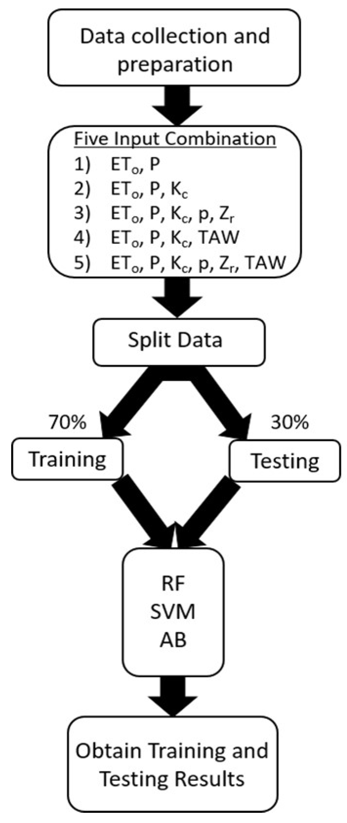
2.5. Input Scenarios and Model Development

Three different machine learning methods (RF, SVM and AB) were applied to simulate and estimate daily potato evapotranspiration under three irrigation regimes (I₁₀₀, I₅₀ and I₀). Weather data (reference evapotranspiration and precipitation), crop data (crop coefficient, water stress threshold (p)—fraction of total available water and root depth) and soil data (the total soil available water) were used as inputs.

Table 3. Summary of scenarios of input data for each machine learning method.

Model	Climate Data		Crop Data			Soil Data
	ETo	P	Kc	p	Zr	TAW
RF1	√	√
RF2	√	√	√
RF3	√	√	√	√	√
RF4	√	√	√			√
RF5	√	√	√	√	√	√
SVM1	√	√
SVM2	√	√	√
SVM3	√	√	√	√	√
SVM4	√	√	√			√
SVM5	√	√	√	√	√	√
AB1	√	√
AB2	√	√	√
AB3	√	√	√	√	√
AB4	√	√	√			√
AB5	√	√	√	√	√	√

ET_o is reference evapotranspiration, P is precipitation, K_c is crop coefficient, p is the fraction of total available water, Z_r is root depth and TAW is the total soil available water.

summarises the input scenarios of data availability applied for each model. RF1, SVM1 and AB1 were fed only with weather data (ETo and P); RF2, SVM2 and AB2 were fed with weather data (ETo and P) and limited crop data (Kc); RF3, SVM3 and AB3 were fed with weather data (ETo and P) and full crop data (Kc, p and Zr); RF4, SVM4 and AB4 were fed with climate data (ETo and P), limited crop data (Kc) and soil data (TAW); and RF5, SVM5 and AB5 were fed with complete data, including weather data (ETo and P), crop data (Kc, p and Zr) and soil data (TAW). The aim of developing these scenarios was to assess the performance metrics of the selected machine learning methods under diverse input data availability, as often encountered in practical applications.

To improve the modelling performance, standardisation was applied to all datasets using the following equation:

$$\mathrm{z}=\frac{\mathrm{x}-\mathsf{\mu }}{\mathsf{\sigma }}$$

(4)

where $\mathsf{\sigma }$ represents the standard deviation value from the average, µ is the average value and x is the observed value.

Total data from 2009–2010 of daily ETc under three irrigation regimes (I₁₀₀, I₅₀ and I₀) were utilised, with 70% randomly selected for training and 30% for testing. Additionally, 5 k-fold cross-validation was employed. The workflow of the modelling procedure for daily potato ETc estimation is depicted in Figure 2.

2.6. Statistical Evaluation

The performance metrics of three machine learning models for comparing observed and simulated ETc-adj values were evaluated using the mean absolute error (MAE), mean squared error (MSE), root mean square error (RMSE), modelling efficiency (EF), slope and coefficient of determination (R²).

$$\mathrm{M}\mathrm{A}\mathrm{E}=\left|\frac{{\sum }_{\mathrm{i}=1}^{\mathrm{n}}({\mathrm{S}}_{\mathrm{i}}-{\mathrm{O}}_{\mathrm{i}})}{\mathrm{n}}\right|$$

(5)

$$\mathrm{M}\mathrm{S}\mathrm{E}=\frac{{\sum }_{\mathrm{i}=1}^{\mathrm{n}}{({\mathrm{S}}_{\mathrm{i}}-{\mathrm{O}}_{\mathrm{i}})}^2}{\mathrm{n}}$$

(6)

$$\mathrm{R}\mathrm{M}\mathrm{S}\mathrm{E}=\sqrt{\frac{{\sum }_{\mathrm{i}=1}^{\mathrm{n}}{({\mathrm{S}}_{\mathrm{i}}-{\mathrm{O}}_{\mathrm{i}})}^2}{\mathrm{n}}}$$

(7)

$$\mathrm{E}\mathrm{F}=1.0-\frac{{\sum }_{\mathrm{ı}=1}^{\mathrm{n}}{({\mathrm{O}}_{\mathrm{i}}-{\mathrm{S}}_{\mathrm{i}})}^2}{{\sum }_{\mathrm{ı}=1}^{\mathrm{n}}{({\mathrm{O}}_{\mathrm{i}}-\overline{\mathrm{O}})}^2}$$

(8)

$${\mathrm{R}}^2=\frac{{\sum }_{\mathrm{ı}=1}^{\mathrm{n}}{({\mathrm{S}}_{\mathrm{i}}-\overline{\mathrm{S}})}^2{({\mathrm{O}}_{\mathrm{i}}-\overline{\mathrm{O}})}^2}{{\sum }_{\mathrm{ı}=1}^{\mathrm{n}}{({\mathrm{S}}_{\mathrm{i}}-\overline{\mathrm{S}})}^2{\sum }_{\mathrm{ı}=1}^{\mathrm{n}}{({\mathrm{O}}_{\mathrm{i}}-\overline{\mathrm{O}})}^2}$$

where $\overline{\mathrm{S}}$ and $\overline{\mathrm{O}}$ are the mean value of the estimated and observed values and S_i and O_i are estimated and observed values, respectively.

3. Results and Discussion

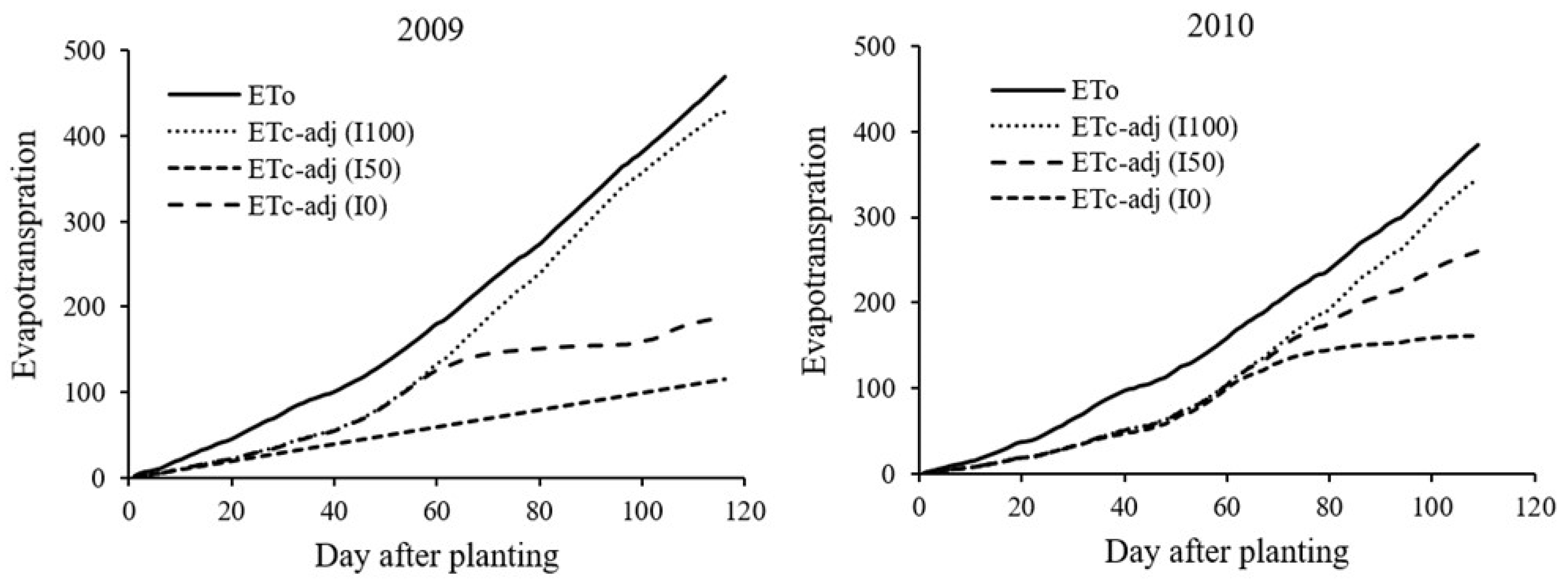
3.1. Crop Evapotranspiration under Different Water Supply and Water Stress

The cumulative ETo and potato crop evapotranspiration under three water regimes are presented in Figure 3 for two growing seasons under consideration. The values of ETo and ETc (I₁₀₀) were higher in 2009 compared to 2010, attributed to greater air temperature and solar radiation in 2009 relative to 2010 (Table 1). Indeed, air temperature and solar radiation are the variables with the most significant influence on reference evapotranspiration and crop ET under optimal water supply [53]. However, in cases of nonoptimal water supply and water deficit in the root zone, ETc-adj (I₅₀) and ETc-adj (I₀) were notably affected by precipitation patterns and crop and soil characteristics. Under water stress treatments, crop evapotranspiration values of I₅₀ and I₀ were lower in 2009 than in 2010. This discrepancy can be attributed to an unfavourable precipitation pattern and higher overall evaporative demand in 2009 compared to 2010, which had a greater impact on potato crop growth under water deficit and affected ETc adj (I₅₀) and ETc adj (I₀) more in that year than in 2010. In 2009, water stress for rainfed crops commenced approximately 25 days after sowing, while, in 2010, it occurred approximately 60 days after sowing. Regarding I50 treatments, water stress began about two weeks earlier in 2009 than in 2010 (Figure 3). Despite higher precipitation in 2009 compared to 2010 (272.2 vs. 170.8 mm), its irregular distribution during the growing season had a greater impact on crops grown under water deficit in 2009 than in 2010. This observation aligns with Cantore et al. [25].

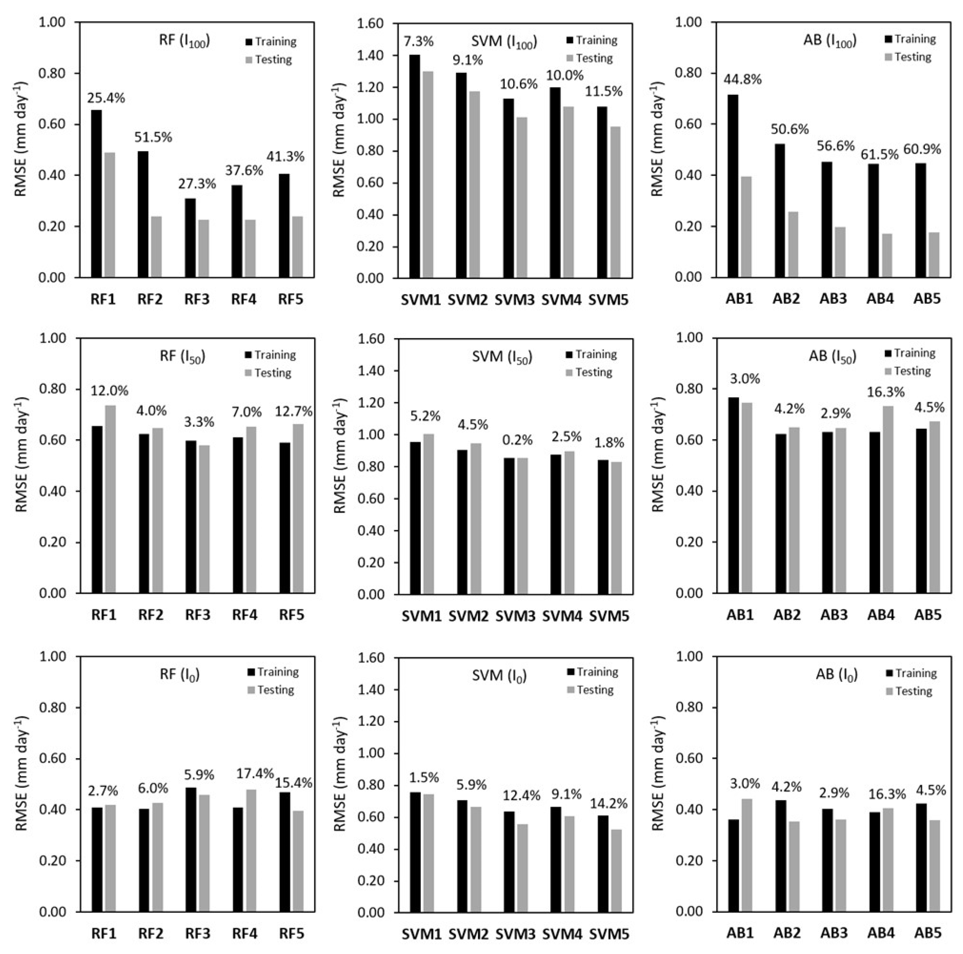
3.2. Assessment of Performances of Machine Learning Methods under Different Irrigation Regimes

The machine learning methods (RF, SVM and AB) were evaluated with five scenarios of climate, crop and soil input data. All the results of modelling performance are shown in Table 4, Table 5 and Table 6 for optimal irrigation, 50% irrigation and rainfed conditions, respectively. The scatter plots of simulated crop evapotranspiration values by the RF, SVM and AB models compared to the ET values obtained by the FAO 56 procedure are presented in Figure 4, Figure 5 and Figure 6 for three water regimes (I₁₀₀, I₅₀ and I₀), respectively. Similarly, the residual plots of crop evapotranspiration values by the RF, SVM and AB models are compared with the crop ET calculated by the FAO 56 method in Figure 7, Figure 8 and Figure 9 for I₁₀₀, I₅₀ and I₀, respectively.

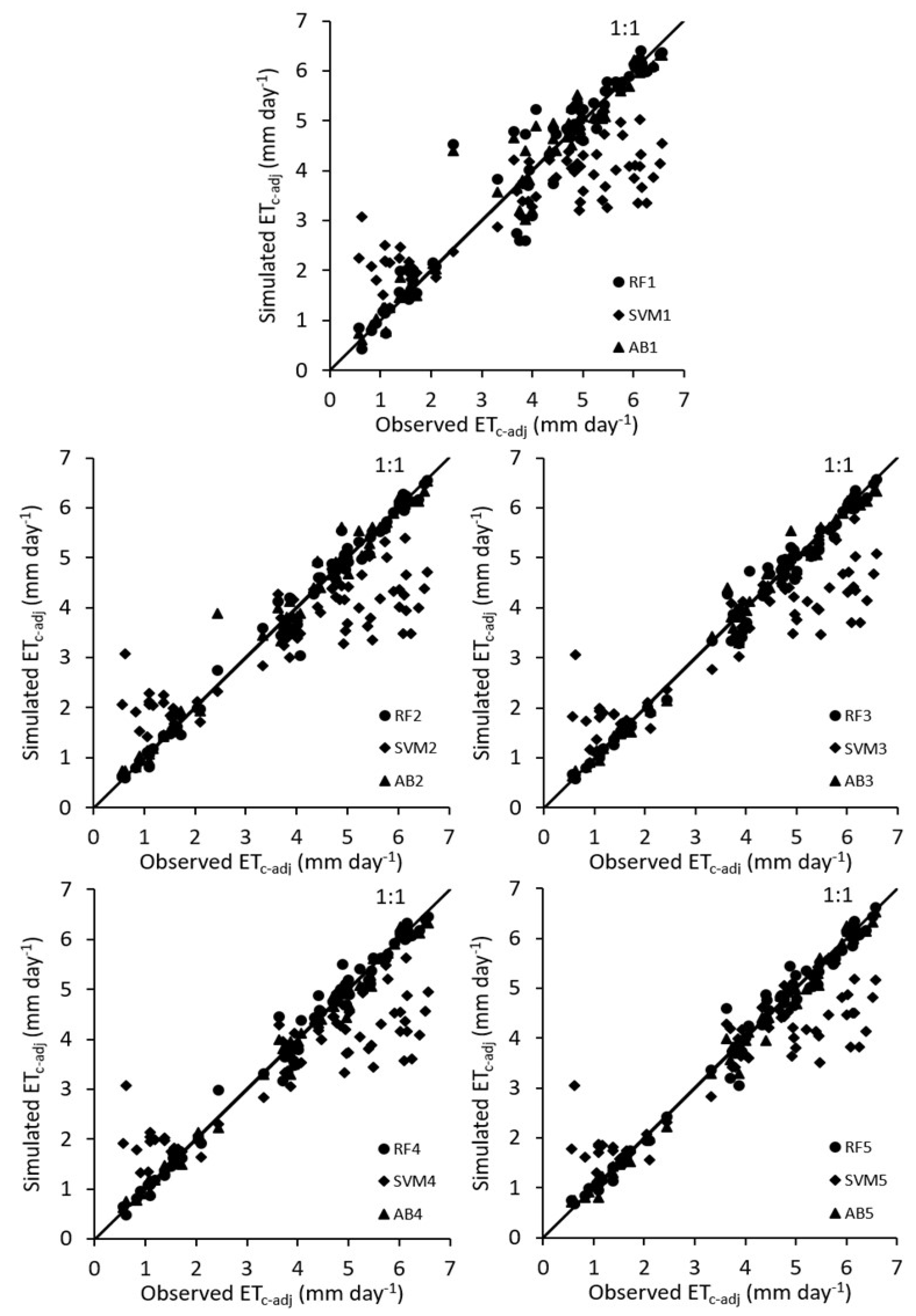
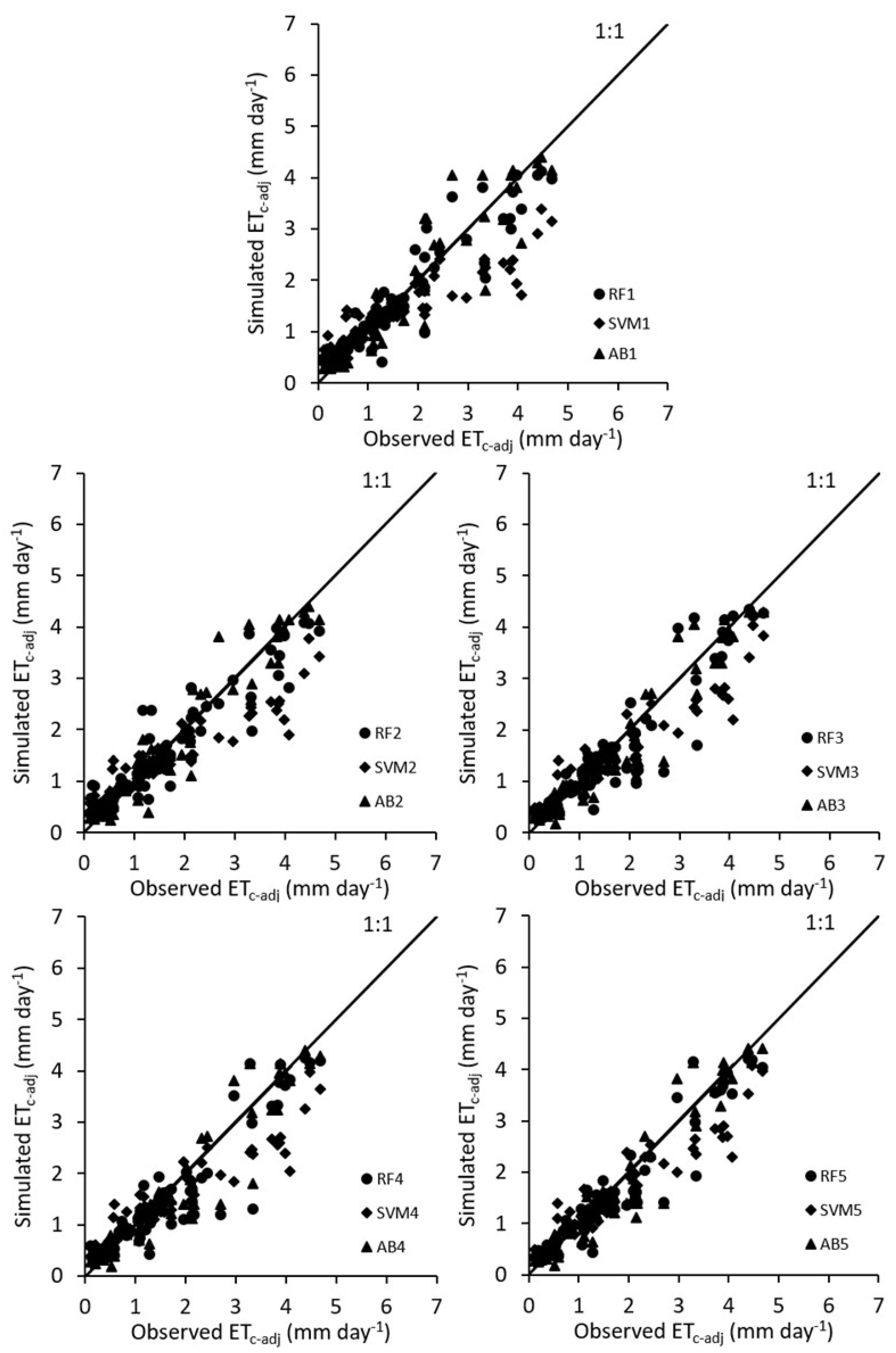
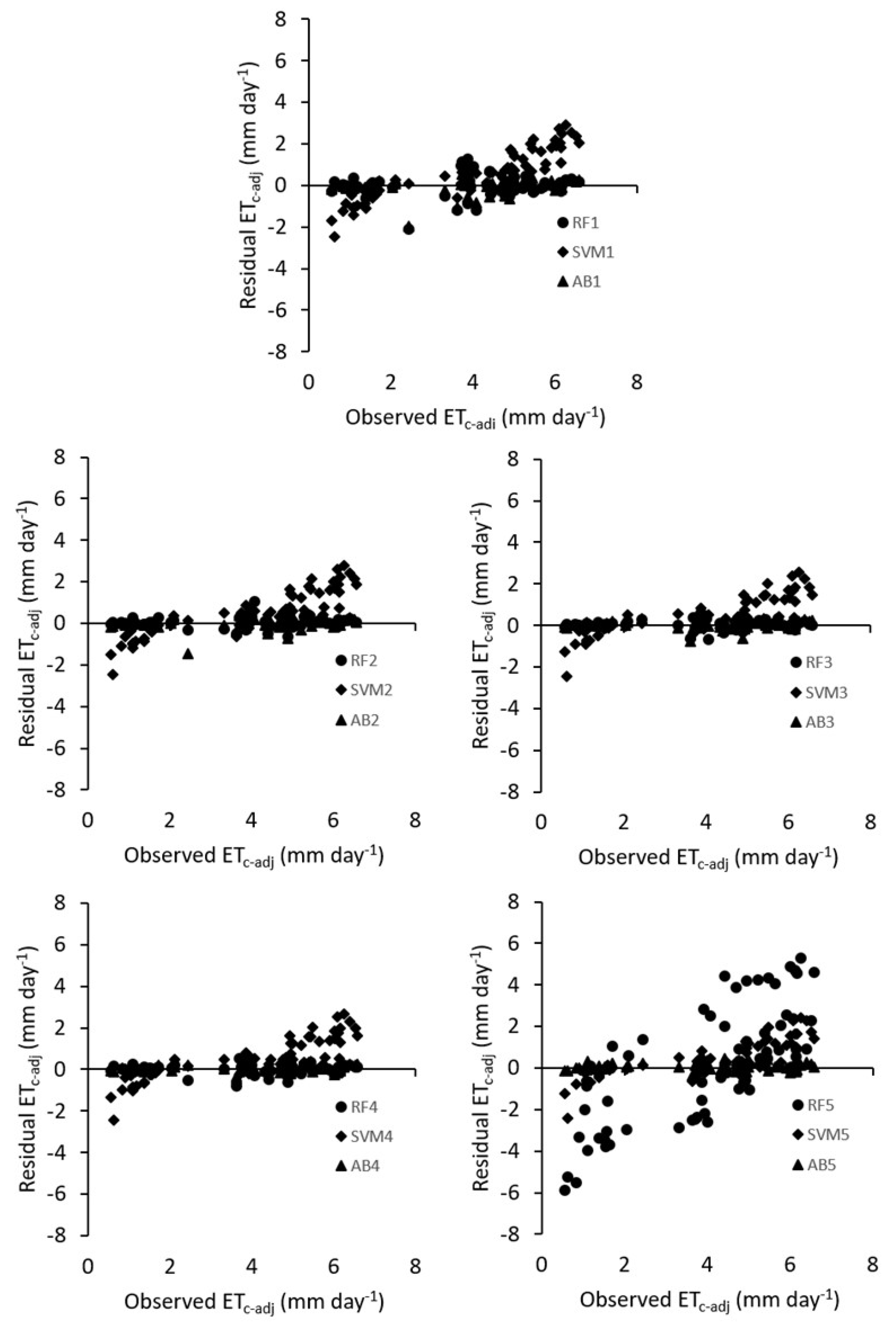
3.2.1. Performances of Machine Learning Methods under Optimal Irrigation Regime (I₁₀₀)

The statistical results of crop evapotranspiration estimate under optimal irrigation (I₁₀₀) using RF, SVM and AB models with five scenarios of climate, crop and soil input data are presented in Table 4 for training and testing subsets. The estimated ETc (I₁₀₀) values varied significantly according to model types and input data availability scenarios. In general, among the scenarios, the SVM model showed the weakest performance confirmed with the lowest R² and EF and the highest MSE, RMSE and MAE in all scenarios for training and testing subsets. In contrast, the AB model for the first (AB1), third (AB3), fourth (AB4) and fifth (AB5) scenario obtained better statistical performance compared to the other two models. For the second scenario, fed with climate data (ETo and P) and limited crop data (Kc), the RF2 model demonstrated the best performance.

Table 4. Performance metrics of applied machine learning methods for estimation of daily potato evapotranspiration for training and testing subset under optimal irrigation regime (I₁₀₀) and five input data scenarios.

Input/Model	Training						Testing
	MAE	RMSE	MSE	Slope	EF	R2	MAE	RMSE	MSE	EF	Slope	R2
	(mm Day−1)	(mm Day−1)	(mm Day−1)				(mm Day−1)	(mm Day−1)	(mm Day−1)
ETo, P
RF1	0.390	0.657	0.431	0.985	0.886	0.887	0.308	0.490	0.240	0.931	0.956	0.933
SVM1	1.140	1.402	1.965	1.957	0.482	0.637	1.053	1.299	1.686	0.512	1.689	0.723
AB1	0.377	0.717	0.514	0.961	0.864	0.866	0.254	0.396	0.157	0.955	0.992	0.956
ETo, P, Kc
RF2	0.225	0.495	0.245	1.006	0.935	0.935	0.163	0.240	0.057	0.983	0.987	0.984
SVM2	1.030	1.290	1.663	1.738	0.562	0.688	0.919	1.173	1.377	0.601	1.507	0.760
AB2	0.228	0.522	0.272	0.998	0.928	0.928	0.158	0.258	0.066	0.981	1.003	0.981
ETo, P, Kc, p, Zr
RF3	0.191	0.311	0.097	1.016	0.974	0.975	0.161	0.226	0.051	0.985	0.991	0.986
SVM3	0.879	1.130	1.278	1.517	0.663	0.753	0.748	1.010	1.021	0.704	1.315	0.798
AB3	0.210	0.452	0.204	1.002	0.946	0.946	0.132	0.196	0.038	0.989	0.996	0.989
ETo, P, Kc, TAW
RF4	0.192	0.362	0.131	1.018	0.965	0.966	0.156	0.226	0.051	0.985	0.988	0.985
SVM4	0.945	1.200	1.440	1.608	0.621	0.727	0.820	1.080	1.166	0.662	1.389	0.781
AB4	0.208	0.444	0.197	1.002	0.948	0.948	0.125	0.171	0.029	0.992	1.004	0.992
ETo, P, Kc, p, Zr, TAW
RF5	0.212	0.407	0.166	1.000	0.956	0.956	0.161	0.239	0.057	0.983	0.993	0.984
SVM5	0.829	1.077	1.159	1.448	0.695	0.771	0.693	0.953	0.908	0.737	1.263	0.812
AB5	0.209	0.447	0.200	1.002	0.947	0.947	0.132	0.175	0.031	0.991	1.008	0.991

Table 4. Performance metrics of applied machine learning methods for estimation of daily potato evapotranspiration for training and testing subset under optimal irrigation regime (I₁₀₀) and five input data scenarios.

Input/Model	Training						Testing
	MAE	RMSE	MSE	Slope	EF	R2	MAE	RMSE	MSE	EF	Slope	R2
	(mm Day−1)	(mm Day−1)	(mm Day−1)				(mm Day−1)	(mm Day−1)	(mm Day−1)
ETo, P
RF1	0.390	0.657	0.431	0.985	0.886	0.887	0.308	0.490	0.240	0.931	0.956	0.933
SVM1	1.140	1.402	1.965	1.957	0.482	0.637	1.053	1.299	1.686	0.512	1.689	0.723
AB1	0.377	0.717	0.514	0.961	0.864	0.866	0.254	0.396	0.157	0.955	0.992	0.956
ETo, P, Kc
RF2	0.225	0.495	0.245	1.006	0.935	0.935	0.163	0.240	0.057	0.983	0.987	0.984
SVM2	1.030	1.290	1.663	1.738	0.562	0.688	0.919	1.173	1.377	0.601	1.507	0.760
AB2	0.228	0.522	0.272	0.998	0.928	0.928	0.158	0.258	0.066	0.981	1.003	0.981
ETo, P, Kc, p, Zr
RF3	0.191	0.311	0.097	1.016	0.974	0.975	0.161	0.226	0.051	0.985	0.991	0.986
SVM3	0.879	1.130	1.278	1.517	0.663	0.753	0.748	1.010	1.021	0.704	1.315	0.798
AB3	0.210	0.452	0.204	1.002	0.946	0.946	0.132	0.196	0.038	0.989	0.996	0.989
ETo, P, Kc, TAW
RF4	0.192	0.362	0.131	1.018	0.965	0.966	0.156	0.226	0.051	0.985	0.988	0.985
SVM4	0.945	1.200	1.440	1.608	0.621	0.727	0.820	1.080	1.166	0.662	1.389	0.781
AB4	0.208	0.444	0.197	1.002	0.948	0.948	0.125	0.171	0.029	0.992	1.004	0.992
ETo, P, Kc, p, Zr, TAW
RF5	0.212	0.407	0.166	1.000	0.956	0.956	0.161	0.239	0.057	0.983	0.993	0.984
SVM5	0.829	1.077	1.159	1.448	0.695	0.771	0.693	0.953	0.908	0.737	1.263	0.812
AB5	0.209	0.447	0.200	1.002	0.947	0.947	0.132	0.175	0.031	0.991	1.008	0.991

The RF model demonstrated very good and stable performance for all scenarios of climate, crop and soil input data (RF1, RF2, RF3, RF4 and RF5). The lowest modelling performance was observed when ETc (I₁₀₀) was predicted only with climate input data (RF1). In the case of RF, significant improvement of ETc (I₁₀₀) was detected for the second scenario when Kc input data are added together with climate data. For this scenario (RF2), the statistical parameters MSE, RMSE, MAE, EF, R² and slope were found to be 0.057 mm day⁻¹, 0.240 mm day⁻¹, 0.163 mm day⁻¹, 0.983, 0.984 and 0.987, respectively, in the testing subset. Then, after adding additional input data (scenarios 3, 4 and 5), the performance of RF models did not improve and the statistical parameters showed similar performance. Among different scenarios, the highest performance was observed for the third scenario with climate (ETo and P) and crop (Kc, p and Zr) input data. The statistical indicators demonstrated similar performances of the RF model for the second (RF2) and fifth (RF5) scenario of input data. The good performance of the RF model to estimate sugar beet evapotranspiration under semi-arid conditions is reported by Yamaç [45]. Similar conclusions were presented recently by Ferreira et al. [69], who used RF algorithm to estimate meteorological data and reference evapotranspiration in Brazil.

The performance of the SVM model slightly improved with the increase in input data (from scenario 1 to scenario 5). However, this model showed poor performance for all scenarios of data availability, indicating its limited suitability for the prediction of crop evapotranspiration. The statistical performance of SVM5 model for ETc (I100) estimation showed the best performance with R² (0.812), EF (0.737), slope (1.263), MSE (0.908 mm day⁻¹), RMSE (0.953 mm day⁻¹) and MAE (0.693 mm day⁻¹) for the testing subset. A general overestimation of ETc was observed for all scenarios and for both training and testing subsets.

The AB model demonstrated the best performance. The poorest performance of the AB model was for the first scenario of data availability (AB1) with MAE, MSE, RMSE, EF, R² and slope equal to 0.254 mm day⁻¹, 0.157 mm day⁻¹, 0.396 mm day⁻¹, 0.955, 0.956 and 0.992, respectively. Nevertheless, even for this scenario, the performance of the AB model was several times better (especially in terms of RMSE) than the performance of SVM with a full dataset (scenario 5). The performance of the AB model improved significantly for the second scenario (AB2) in the testing subset. The model was slightly improved in the third, fourth and fifth scenarios. The AB model showed the superlative performance for ETc (I₁₀₀) estimate when scenario 4 with inputs of climate, crop and soil data was used with R² of 0.992, EF of 0.992, slope of 1.004, MAE of 0.125 mm day⁻¹, MSE of 0.029 mm day⁻¹ and RMSE of 0.171 mm day⁻¹.

A comparison of observed and simulated ETc (I₁₀₀) values for RF, SVM and AB models are presented in Figure 4 for different scenarios. The SVM model created more scattered points than the other machine learning models, while the AB model produced the lowest scattering of estimates in comparison to other machine learning models. These results confirmed that the performance of the SVM models was poorer than that of AB and RF models. The residual plots of ETc (I₁₀₀) values by RF, SVM and AB models are shown in Figure 8. The residual plot showed that the most errors occurred for scenario 1, while the least errors occurred for scenario 5. This is in agreement with the availability of input data and obtained statistical parameters.

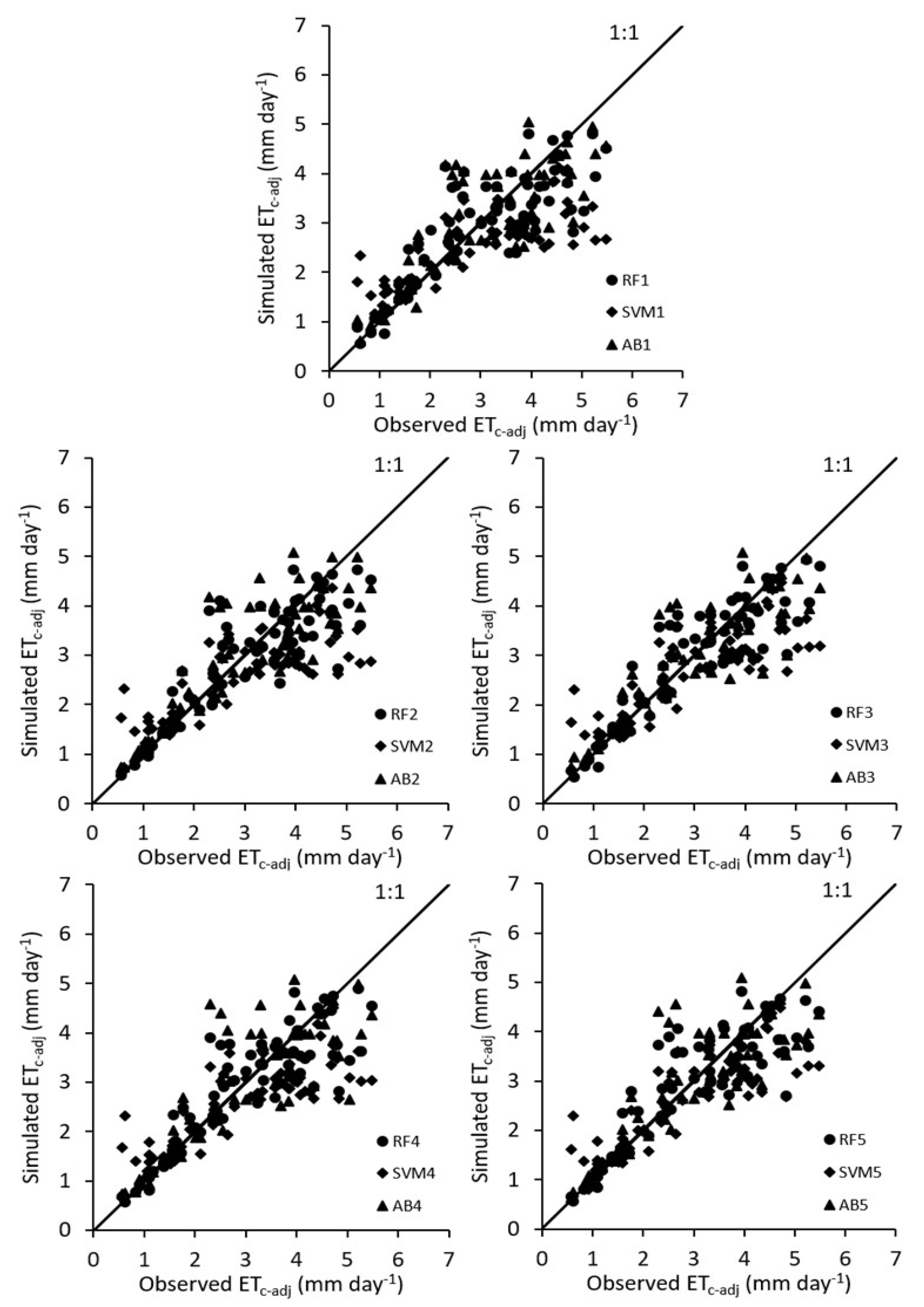
3.2.2. Performance of Machine Learning Methods under 50% of Optimal Irrigation Regime (I₅₀)

The statistical results of crop evapotranspiration under 50% of optimal irrigation supply (I₅₀) using RF, SVM and AB models with five scenarios of climate, soil and crop input data are shown in Table 5. Generally, the RF model exhibited the highest statistical performances in both the training and testing subsets for all input scenarios compared to the SVM and AB models. Similarly to the previous case of optimal water supply, the SVM models demonstrated the poorest statistical performance in both the training and testing subsets for all input scenarios.

Table 5. Performance metrics of applied machine learning methods for estimation of daily potato evapotranspiration for training and testing subset under 50% of optimal irrigation regime (I₅₀) and five input data scenarios.

Input/Model	Training						Testing
	MAE	RMSE	MSE	Slope	EF	R2	MAE	RMSE	MSE	Slope	EF	R2
	(mm Day−1)	(mm Day−1)	(mm Day−1)				(mm Day−1)	(mm Day−1)	(mm Day−1)
ETo, P
RF1	0.462	0.656	0.430	0.948	0.741	0.743	0.531	0.735	0.540	0.996	0.702	0.706
SVM1	0.739	0.957	0.915	1.755	0.449	0.556	0.777	1.007	1.015	1.522	0.440	0.604
AB1	0.527	0.768	0.589	0.902	0.645	0.653	0.548	0.745	0.555	0.946	0.694	0.697
ETo, P, Kc
RF2	0.414	0.623	0.389	0.964	0.766	0.767	0.437	0.648	0.420	1.019	0.768	0.777
SVM2	0.690	0.906	0.820	1.557	0.506	0.585	0.724	0.947	0.896	1.389	0.506	0.637
AB2	0.413	0.624	0.389	0.976	0.766	0.766	0.470	0.650	0.422	0.977	0.767	0.768
ETo, P, Kc, p, Zr
RF3	0.401	0.599	0.359	1.007	0.784	0.784	0.405	0.579	0.335	0.999	0.815	0.816
SVM3	0.641	0.855	0.730	1.372	0.560	0.609	0.653	0.857	0.734	1.308	0.595	0.698
AB3	0.406	0.630	0.397	0.969	0.761	0.762	0.447	0.648	0.419	1.010	0.769	0.775
ETo, P, Kc, TAW
RF4	0.411	0.610	0.373	0.967	0.776	0.777	0.441	0.653	0.427	1.007	0.765	0.772
SVM4	0.661	0.874	0.764	1.447	0.540	0.602	0.683	0.896	0.803	1.317	0.557	0.665
AB4	0.480	0.630	0.396	0.994	0.761	0.761	0.473	0.733	0.537	0.914	0.704	0.711
ETo, P, Kc, p, Zr, TAW
RF5	0.381	0.589	0.346	1.015	0.791	0.791	0.462	0.664	0.441	1.001	0.756	0.760
SVM5	0.628	0.843	0.710	1.322	0.572	0.613	0.629	0.828	0.686	1.292	0.622	0.716
AB5	0.426	0.644	0.414	0.962	0.750	0.752	0.454	0.673	0.453	0.955	0.750	0.753

Table 5. Performance metrics of applied machine learning methods for estimation of daily potato evapotranspiration for training and testing subset under 50% of optimal irrigation regime (I₅₀) and five input data scenarios.

Input/Model	Training						Testing
	MAE	RMSE	MSE	Slope	EF	R2	MAE	RMSE	MSE	Slope	EF	R2
	(mm Day−1)	(mm Day−1)	(mm Day−1)				(mm Day−1)	(mm Day−1)	(mm Day−1)
ETo, P
RF1	0.462	0.656	0.430	0.948	0.741	0.743	0.531	0.735	0.540	0.996	0.702	0.706
SVM1	0.739	0.957	0.915	1.755	0.449	0.556	0.777	1.007	1.015	1.522	0.440	0.604
AB1	0.527	0.768	0.589	0.902	0.645	0.653	0.548	0.745	0.555	0.946	0.694	0.697
ETo, P, Kc
RF2	0.414	0.623	0.389	0.964	0.766	0.767	0.437	0.648	0.420	1.019	0.768	0.777
SVM2	0.690	0.906	0.820	1.557	0.506	0.585	0.724	0.947	0.896	1.389	0.506	0.637
AB2	0.413	0.624	0.389	0.976	0.766	0.766	0.470	0.650	0.422	0.977	0.767	0.768
ETo, P, Kc, p, Zr
RF3	0.401	0.599	0.359	1.007	0.784	0.784	0.405	0.579	0.335	0.999	0.815	0.816
SVM3	0.641	0.855	0.730	1.372	0.560	0.609	0.653	0.857	0.734	1.308	0.595	0.698
AB3	0.406	0.630	0.397	0.969	0.761	0.762	0.447	0.648	0.419	1.010	0.769	0.775
ETo, P, Kc, TAW
RF4	0.411	0.610	0.373	0.967	0.776	0.777	0.441	0.653	0.427	1.007	0.765	0.772
SVM4	0.661	0.874	0.764	1.447	0.540	0.602	0.683	0.896	0.803	1.317	0.557	0.665
AB4	0.480	0.630	0.396	0.994	0.761	0.761	0.473	0.733	0.537	0.914	0.704	0.711
ETo, P, Kc, p, Zr, TAW
RF5	0.381	0.589	0.346	1.015	0.791	0.791	0.462	0.664	0.441	1.001	0.756	0.760
SVM5	0.628	0.843	0.710	1.322	0.572	0.613	0.629	0.828	0.686	1.292	0.622	0.716
AB5	0.426	0.644	0.414	0.962	0.750	0.752	0.454	0.673	0.453	0.955	0.750	0.753

The RF model with only climate data (RF1) indicated the lowest performance with R² (0.706), EF (0.702), slope (0.996), MSE (0.540 mm day⁻¹), RMSE (0.735 mm day⁻¹) and MAE (0.531 mm day⁻¹) obtained for the testing subset. However, the RF models employing climate (ETo and P) and crop (Kc, p and Zr) input data had the highest estimation accuracy when compared with the other scenarios, with MAE, MSE, RMSE, EF, R² and slope equal to 0.405 mm day⁻¹, 0.335 mm day⁻¹, 0.579 mm day⁻¹, 0.815, 0.816 and 0.999, respectively. As seen from Table 5, the RF model performance increased when crop data were added as input to the weather data. However, no further improvement of ETc_adj estimate was observed when soil input data were added (scenarios 4 and 5). In fact, the value of total available water (TAW) does not provide significant additional information for the estimate of crop evapotranspiration if it is not supported by data about root depth (Zr) and crop optimum yield threshold (p), as is the case of scenario 4.

The statistical result of ETc_adj estimation with the SVM model for five scenarios of input data indicated the highest performance when climate, crop and soil input data were employed for potato ETc_adj (I₅₀) estimation (scenario 5). In that case, R² was 0.716 with a slope of 1.292, EF was 0.622, MAE was 0.629 mm day⁻¹, MSE was 0.686 mm day⁻¹ and RMSE was 0.828 mm day⁻¹ in the testing subset. However, SVM1, fed only with climate data, produced the poorest performance with R² of 0.604, EF of 0.440, a slope of 1.522, MSE of 1.015 mm day⁻¹, RMSE of 1.007 mm day⁻¹ and MAE of 0.777 mm day⁻¹ in the testing subset. Similarly to the case of full irrigation supply, the SVM overestimated ETc_adj for both data subsets and all scenarios of data availability.

The performance of the AB model for estimating potato ETc-adj (I₅₀) values showed that the model fed only with climate data (AB1) had the lowest performance with R² (0.697), EF (0.694), slope (0.946), MSE (0.555 mm day⁻¹), RMSE (0.745 mm day⁻¹) and MAE (0.548 mm day⁻¹) for the testing subset.

The model improved slightly in the second and third scenarios when crop input data were added as input to the climate data. The best performance was observed for the AB3 with inputs of weather (ETo and P) and crop (Kc, p and Zr) variables, with MAE, MSE, RMSE, EF, slope and R² equal to 0.447 mm day⁻¹, 0.419 mm day⁻¹, 0.648 mm day⁻¹, 0.769, 1.010 and 0.775, respectively. The consideration of total available water (TAW) as input did not improve the estimation of ETc_adj.

A comparison of observed and simulated ETc-adj (I₅₀) values for RF, SVM and AB models is presented in Figure 7. The RF, SVM and AB models fed only with climate input data (scenario 1) produced more scattered estimates than for other scenarios of data availability. The ETc-adj (I₅₀) values estimated by RF3, SVM3 and AB3 models were closer to the observed values than other scenarios. This confirms that the RF3, SVM3 and AB3 models can predict ETc-adj (I₅₀) values better than other combinations of input data availability. The residual plots of ETc-adj (I₅₀) values by RF, SVM and AB models are shown in Figure 6. The residual plot showed that the most errors occurred in scenario 1, while the least errors occurred in scenario 3.

3.2.3. Performances of Machine Learning Methods under Rainfed Condition (I0)

The statistical results of ETc-adj estimation under rainfed (I₀) conditions using RF, SVM and AB models with five scenarios of climate, soil and crop input data are presented in Table 6. Among the scenarios, RF1, AB2, AB3, AB4 and AB5 showed the highest performances, while SVM1, SVM2, SVM3, SVM4 and SVM5 demonstrated the poorest performances.

Table 6. Performance metrics of applied machine learning methods for estimation of daily potato evapotranspiration for training and testing subset under rainfed condition (I₀) and five input data scenarios.

Input/Model	Training						Testing
	MAE	RMSE	MSE	Slope	EF	R2	MAE	RMSE	MSE	Slope	EF	R2
	(mm Day−1)	(mm Day−1)	(mm Day−1)				(mm Day−1)	(mm Day−1)	(mm Day−1)
ETo, P
RF1	0.285	0.409	0.167	1.159	0.854	0.870	0.288	0.420	0.176	1.053	0.886	0.889
SVM1	0.525	0.755	0.571	1.933	0.502	0.661	0.517	0.744	0.553	1.768	0.642	0.844
AB1	0.247	0.361	0.130	1.011	0.886	0.887	0.281	0.442	0.195	0.943	0.874	0.877
ETo, P, Kc
RF2	0.280	0.403	0.162	1.219	0.859	0.887	0.305	0.427	0.182	1.074	0.882	0.879
SVM2	0.486	0.706	0.499	1.713	0.565	0.688	0.466	0.664	0.441	1.583	0.715	0.868
AB2	0.271	0.437	0.191	0.995	0.833	0.834	0.243	0.354	0.125	0.975	0.919	0.920
ETo, P, Kc, p, Zr
RF3	0.296	0.488	0.239	0.977	0.792	0.793	0.294	0.459	0.211	0.958	0.864	0.874
SVM3	0.435	0.636	0.405	1.494	0.647	0.730	0.401	0.557	0.310	1.397	0.800	0.898
AB3	0.244	0.404	0.163	0.990	0.858	0.858	0.242	0.361	0.131	0.984	0.916	0.921
ETo, P, Kc, TAW
RF4	0.268	0.408	0.167	1.046	0.855	0.856	0.313	0.479	0.229	1.002	0.852	0.865
SVM4	0.456	0.667	0.445	1.579	0.612	0.711	0.432	0.606	0.367	1.474	0.763	0.883
AB4	0.225	0.389	0.151	0.999	0.868	0.868	0.261	0.406	0.165	0.977	0.893	0.900
ETo, P, Kc, p, Zr, TAW
RF5	0.293	0.469	0.220	1.025	0.808	0.809	0.273	0.397	0.157	1.036	0.898	0.906
SVM5	0.418	0.612	0.375	1.433	0.673	0.744	0.380	0.525	0.275	1.342	0.822	0.904
AB5	0.247	0.423	0.179	0.977	0.844	0.844	0.241	0.359	0.129	0.972	0.917	0.922

Table 6. Performance metrics of applied machine learning methods for estimation of daily potato evapotranspiration for training and testing subset under rainfed condition (I₀) and five input data scenarios.

Input/Model	Training						Testing
	MAE	RMSE	MSE	Slope	EF	R2	MAE	RMSE	MSE	Slope	EF	R2
	(mm Day−1)	(mm Day−1)	(mm Day−1)				(mm Day−1)	(mm Day−1)	(mm Day−1)
ETo, P
RF1	0.285	0.409	0.167	1.159	0.854	0.870	0.288	0.420	0.176	1.053	0.886	0.889
SVM1	0.525	0.755	0.571	1.933	0.502	0.661	0.517	0.744	0.553	1.768	0.642	0.844
AB1	0.247	0.361	0.130	1.011	0.886	0.887	0.281	0.442	0.195	0.943	0.874	0.877
ETo, P, Kc
RF2	0.280	0.403	0.162	1.219	0.859	0.887	0.305	0.427	0.182	1.074	0.882	0.879
SVM2	0.486	0.706	0.499	1.713	0.565	0.688	0.466	0.664	0.441	1.583	0.715	0.868
AB2	0.271	0.437	0.191	0.995	0.833	0.834	0.243	0.354	0.125	0.975	0.919	0.920
ETo, P, Kc, p, Zr
RF3	0.296	0.488	0.239	0.977	0.792	0.793	0.294	0.459	0.211	0.958	0.864	0.874
SVM3	0.435	0.636	0.405	1.494	0.647	0.730	0.401	0.557	0.310	1.397	0.800	0.898
AB3	0.244	0.404	0.163	0.990	0.858	0.858	0.242	0.361	0.131	0.984	0.916	0.921
ETo, P, Kc, TAW
RF4	0.268	0.408	0.167	1.046	0.855	0.856	0.313	0.479	0.229	1.002	0.852	0.865
SVM4	0.456	0.667	0.445	1.579	0.612	0.711	0.432	0.606	0.367	1.474	0.763	0.883
AB4	0.225	0.389	0.151	0.999	0.868	0.868	0.261	0.406	0.165	0.977	0.893	0.900
ETo, P, Kc, p, Zr, TAW
RF5	0.293	0.469	0.220	1.025	0.808	0.809	0.273	0.397	0.157	1.036	0.898	0.906
SVM5	0.418	0.612	0.375	1.433	0.673	0.744	0.380	0.525	0.275	1.342	0.822	0.904
AB5	0.247	0.423	0.179	0.977	0.844	0.844	0.241	0.359	0.129	0.972	0.917	0.922

The modelling performance of RF decreased from scenario 1 to 4 in the testing subset. However, the RF model showed the best performance metrics when all input data, such as climate (ETo and P), crop (Kc, p and Zr) and soil (TAW), were added to the model. As a result, R² was 0.906 with the slope of 1.036, EF of 0.898, MAE of 0.273 mm day⁻¹, MSE of 0.157 mm day⁻¹ and RMSE of 0.397 mm day⁻¹ in the testing subset. Among the other scenarios, the RF4 model, fed with climate (ETo and P), crop (Kc) and soil (TAW) data, has the lowest performance with MAE of 0.273 mm day⁻¹, MSE of 0.157 mm day⁻¹, RMSE of 0.397 mm day⁻¹, EF of 0.898, slope of 1.036 and R² of 0.906, respectively. It can be noticed that crop input data of p and Zr significantly affected the modelling performances of the RF model.

The SVM1 model produced the lowest performance with MAE, MSE, RMSE, EF, slope and R² equal to 0.517 mm day⁻¹, 0.553 mm day⁻¹, 0.744 mm day⁻¹, 0.642, 1.768 and 0.844, respectively, in the testing subset, while the SVM5 model produced the best performance with MAE, MSE, RMSE, EF, slope and R² equal to 0.380 mm day⁻¹, 0.275 mm day⁻¹, 0.525 mm day⁻¹, 0.822, 1.342 and 0.904, respectively. In general, as in the previous cases referring to optimal water supply and deficit irrigation, the SVM model demonstrated the poorest performance, with a strong trend of overestimation of Etc-adj in the range from 34% (scenario 5) to 77% (scenario 1) for the testing subset.

The AB model showed the lowest statistical performance for scenario 1, and this was improved for other scenarios when additional input data were used. Slightly better performance was observed when the model was applied for scenarios 2, 3 and 5 compared to scenario 4, which confirmed the previous findings of this study referring to optimal and deficit irrigation. The statistical parameters of the AB model are similar for the second (AB2), third (AB3) and fifth (AB5) scenario of input data availability. The AB2 model showed the highest statistical performance in the testing subset with RMSE equal to 0.354 mm day⁻¹, MAE was 0.243 mm day⁻¹, EF was 0.919, slope of 0.975 and with R² of 0.920.

An evaluation of simulated and observed ETc-adj (I₀) values for RF, SVM and AB models is shown in Figure 5. In all scenarios, the SVM model indicated a more scattered prediction than other machine learning models, as well as a noticeable overestimation. The ETc-adj (I₀) values estimated by the first scenario of the RF model and second, third, fourth and fifth scenarios of the AB model were closer to the observed values and followed the trend of a 1:1 regression line. These findings agree with statistical indicators (Table 6). The residual plots of ETc-adj (I₀) values by RF, SVM and AB models are shown in Figure 9. The residual plot showed that the most errors occurred in scenario 1, while the least errors occurred for scenarios 3 and 5.

3.3. Assessment of Stability of Machine Learning Methods under Different Irrigation Regimes

The training and testing RMSE values of three water regimes (I₁₀₀, I₅₀ and I₀) are demonstrated in Figure 10 for all the applied machine learning models. In general, the RF and AB models provided better prediction than the SVM model for all input scenarios. The change in testing RMSE over training RMSE is shown in Figure 10. The RF and AB models with all scenarios under optimal irrigation regimes (I₁₀₀) had the largest percentage differences between training and testing RMSE values (from 25.4% to 61.5%). In the case of limited water supply (deficit irrigation and rainfed cultivation), the percentage difference between training and testing RMSE values was small (from 0.2% to 17.4).

In general, the SVM model demonstrated the poorest performance for all elaborated cases. However, it showed the smallest difference of RMSE between training and testing subsets. Moreover, in the case of rainfed potato cultivation, the RMSE of the SVM model was always lower for training than for testing subsets. This confirms that this model has very limited suitability to predict crop evapotranspiration.

4. Discussion

Considering different data availability, the overall results demonstrated that the performance of models was improved with an increasing number of input variables. Nevertheless, the greatest impact on the simulation results was observed when weather data and crop coefficient values were available. The availability of soil characteristics, root depth and fraction of available water had a minor impact on simulation results. The SVM model showed the lowest predicting accuracy in all input scenarios under three water regimes. Substantial overestimation of crop evapotranspiration was observed, indicating low suitability of SVM for the prediction of crop ET.

The AB model offered the best prediction accuracy for four out of five scenarios of data availability, while the RF model offered the best prediction accuracy for the scenario where weather and crop coefficient data were available under optimal irrigation regimes (I₁₀₀). In the case of deficit irrigation and 50% of the optimal irrigation supply (I₅₀), the RF model was superior for all scenarios of data availability. Under the rainfed condition, the RF model fed only with climate data had better prediction accuracy than SVM and AB models. However, the AB model had the best performance for the other four scenarios of data availability. In general, the machine learning models demonstrated better prediction of crop evapotranspiration under rainfed (I₀) and optimal irrigation regimes (I₁₀₀) than under deficit irrigation (50% of the optimal irrigation regime).

In general, the assessment of performances of machine learning methods under different irrigation regimes showed that RF, SVM and AB models were able to simulate complex and nonlinear relationships among the climate, soil and crop parameters and to adequately estimate crop evapotranspiration under different water regimes. This can be explained by the ability of selected models to autonomously solve complex and nonlinear problems by gathering datasets from various sources [70]. The models’ performance improved with an increasing number of input variables [42]. The greatest positive impact on the models’ performance was observed when the crop coefficient data were added to weather data availability (scenario 2).

Under nonlimited water supply, the soil water balance and, therefore, crop evapotranspiration depend substantially only on the weather variables and specific crop growing stage because there is no water stress and crop parameters (root depth, fraction of readily available water and total available water) are not relevant to support crop growth. As water supply is reduced, the importance of the crop’s root depth and availability of water within the root zone increases because they regulate the crop’s response to water and determine the capability of the crop to use water. In fact, under limited water supply, crop evapotranspiration is reduced as a function of water availability in the root zone and crop-specific sensitivity to water stress.

The assessment of stability of machine learning methods under different irrigation regimes revealed the instability of the RF and AB models as they produced changes in prediction accuracy when new input data were applied under optimal irrigation regimes (I₁₀₀). Similar findings were pointed out also by Hassan et al. [71] who mentioned that the RMSE of the RF model had large differences between training and testing values. For all models, the RMSE of the testing subset was lower than for the training subset only in the case of ETc estimate under optimal water supply. For the other two cases (deficit irrigation and rainfed cultivation), the difference in RMSE between training and testing subsets was only 2–3% and, for some scenarios, it was greater for testing than for training subsets. Therefore, it can be concluded that the performance of models is more stable under water stress conditions than under optimal irrigation supply.

5. Conclusions

This study focused on the suitability of three machine learning algorithms (RF, SVM and AB models) to predict daily potato evapotranspiration under optimal and limited water supply and five scenarios of data availability. To the best of the authors’ knowledge, the machine learning methods (RF, SVM and AB) were firstly studied to estimate daily ET under limited water supply and water stress conditions (ETc-adj), which is particularly relevant for arid and semi-arid areas.

The presented results are particularly useful for sustainable and efficient management of irrigation in areas where water resources are scarce and input data are limited to few weather, crop and soil parameters. In these situations, the application of machine learning models is of great importance to fill the gap of limited data availability to estimate crop evapotranspiration and improve irrigation scheduling.

Future studies are needed to evaluate the performance of different machine learning models for ETc-adj estimation under different environments and various scenarios of climate, crop and soil input data. Particular attention should be given to the ET estimate from tree crops with fixed root depth, which might facilitate the application of machine learning algorithms in irrigation scheduling.

References

1. Fader, M.; Giupponi, C.; Burak, S.; Dakhlaoui, H.; Koutroulis, A.; Lange, M.A.; Llasat, M.C.; Pulido-Velazquez, D.; Sanz-Cobeña, A. Water. In Climate and Environmental Change in the Mediterranean Basin—Current Situation and Risks for the Future. First Mediterranean Assessment Report; Cramer, W., Guiot, J., Marini, K., Eds.; Union for the Mediterranean; Plan Bleu; UNEP/MAP: Marseille, France, 2020; pp. 181–236. [Google Scholar]
2. Savin, R.; Cossani, C.M.; Dahan, R.; Ayad, J.Y.; Albrizio, R.; Todorovic, M.; Karrou, M.; Slafer, G.A. Intensifying cereal management in dryland Mediterranean agriculture: Rainfed wheat and barley responses to nitrogen fertilisation. Eur. J. Agron. 2022, 137, 126518. [Google Scholar]
3. Gao, Z.Z.; Wang, C.; Zhao, J.C. Adopting different irrigation and nitrogen management based on precipitation year types balances winter wheat yields and greenhouse gas emissions. Field Crops Res. 2022, 280, 108484. [Google Scholar] [CrossRef]
4. Todorovic, M.; Jovanovic, N. Climate change and Agriculture. In Encyclopedia of Water: Science, Technology, and Society; Maurice, P.A., Ed.; John Wiley & Sons, Inc.: Hoboken, NJ, USA, 2019; Volume 209, pp. 2463–2478. [Google Scholar]
5. Core Writing Team; Lee, H.; Romero, J. (Eds.) IPCC Climate Change 2023: Synthesis Report. In Contribution of Working Groups I, II and III to the Sixth Assessment Report of the Intergovernmental Panel on Climate Change; IPCC: Geneva, Switzerland, 2023; pp. 35–115. [Google Scholar]
6. Cramer, W.; Guiot, J.; Marini, K. (Eds.) MedECC Climate and Environmental Change in the Mediterranean Basin—Current Situation and Risks for the Future. In First Mediterranean Assessment Report; Union for the Mediterranean; Plan Bleu; UNEP/MAP: Marseille, France, 2020; Volume 632, ISBN 978-2-9577416-0-1. [Google Scholar]
7. Tanasijevic, L.; Todorovic, M.; Pereira, L.S.; Pizzigalli, C.; Lionello, P. Impacts of climate change on olive crop evapotranspiration and irrigation requirements in the Mediterranean region. Agric. Water Manag. 2014, 144, 54–68. [Google Scholar]
8. Saadi, S.; Todorovic, M.; Tanasijevic, L.; Pereira, L.S.; Pizzigalli, C.; Lionello, P. Climate change and Mediterranean agriculture: Impacts on winter wheat and tomato crop evapotranspiration, irrigation requirements and yield. Agric. Water Manag. 2015, 147, 103–115. [Google Scholar] [CrossRef]
9. Knezevic, M.; Zivotic, L.; Cerekovic, N.; Topalovic, A.; Kokovic, N.; Todorovic, M. Impact of climate change on water requirements and growth of potato in different climatic zones of Montenegro. J. Water Clim. Chang. 2018, 9, 657–671. [Google Scholar]
10. Todorovic, M. Climate Change and Mediterranean agriculture: Expected impacts, possible solutions and the way forward. In Crises Et Conflits En Méditerranée: L’agriculture Comme Résilience; Lacirignola, C., Ed.; La Bibliothèque de l’iReMMO (Institut De Recherche Et D’études Méditerranée Moyen-Orient); L’Harmattan: Paris, France, 2018; pp. 13–28. [Google Scholar]
11. Yang, X.; Li, Z.; Cui, S.; Cao, Q.; Deng, J.; Lai, X.; Shen, Y. Cropping system productivity and evapotranspiration in the semiarid Loess Plateau of China under future temperature and precipitation changes: An APSIM-based analysis of rotational vs. continuous systems. Agric. Water Manag. 2020, 229, 105959. [Google Scholar] [CrossRef]
12. Jovanovic, N.; Pereira, L.S.; Paredes, P.; Pôças, I.; Cantore, V.; Todorovic, M. A review of strategies, methods and technologies to reduce non-beneficial consumptive water use on farms considering the FAO56 methods. Agric. Water Manag. 2020, 239, 106267. [Google Scholar]
13. Farrell, A.D.; Deryng, D.; Neufeldt, H. Modelling adaptation and transformative adaptation in cropping systems: Recent advances and future directions. Curr. Opin. Environ. Sustain. 2023, 61, 101265. [Google Scholar] [CrossRef]
14. Dettori, M.; Cesaraccio, C.; Duce, P. Simulation of climate change impacts on production and phenology of durum wheat in Mediterranean environments using CERES-Wheat model. Field Crops Res. 2017, 206, 43–53. [Google Scholar]
15. Fabeiro, C.; Martin de Santa Olalla, F.; de Juan, J.A. Yield and size of deficit irrigated potatoes. Agric. Water Manag. 2001, 48, 255–266. [Google Scholar] [CrossRef]
16. Ali, S.; Xu, Y.Y.; Jia, Q.M.; Ma, X.C.; Ahmad, I.; Adnan, M.; Gerard, R.; Ren, X.L.; Zhang, P.; Cai, T.; et al. Interactive effects of plastic film mulching with supplemental irrigation on winter wheat photosynthesis, chlorophyll fluorescence and yield under simulated precipitation conditions. Agric. Water Manag. 2018, 207, 1–14. [Google Scholar] [CrossRef]
17. Wang, J.; Ghimire, R.; Fu, X.; Sainju, U.M.; Liu, W. Straw mulching increases precipitation storage rather than water use efficiency and dryland winter wheat yield. Agric. Water Manag. 2018, 106, 95–101. [Google Scholar]
18. Candido, V.; Cantore, V.; Castronuovo, D.; Denora, M.; Schiattone, M.I.; Sergio, L.; Todorovic, M.; Boari, F. Effect of Water Regime, Nitrogen Level, and Biostimulant Application on the Water and Nitrogen Use Efficiency of Wild Rocket [Diplotaxis tenuifolia (L.) DC]. Agronomy 2023, 13, 507. [Google Scholar]
19. Van Oosten, M.J.; Pepe, O.; De Pascale, S.; Silletti, S.; Maggio, A. The role of biostimulants and bioeffectors as alleviators of abiotic stress in crop plants. Chem. Biol. Technol. Agric. 2017, 4, 5. [Google Scholar]
20. Caradonia, F.; Ronga, D.; Tava, A.; Francia, E. Plant Biostimulants in Sustainable Potato Production: An Overview. Potato Res. 2022, 65, 83–104. [Google Scholar]
21. Schiattone, M.I.; Boari, F.; Cantore, V.; Castronuovo, D.; Denora, M.; Di Venere, D.; Perniola, M.; Sergio, L.; Todorovic, M.; Candido, V. Effect of water regime, nitrogen level and biostimulants application on yield and quality traits of wild rocket [Diplotaxis tenuifolia (L.) DC.]. Agric. Water Manag. 2023, 277, 108078. [Google Scholar]
22. El Boukhari, M.E.M.; Barakate, M.; Bouhia, Y.; Lyamlouli, K. Trends in seaweed extract based biostimulants: Manufacturing process and beneficial effect on soil-plant systems. Plants 2020, 9, 359. [Google Scholar] [CrossRef]
23. Abi Saab, M.T.; Jomaa, I.; Skaf, S.; Fahed, S.; Todorovic, M. Assessment of a Smartphone Application for Real-Time Irrigation Scheduling in Mediterranean Environments. Water 2019, 11, 252. [Google Scholar]
24. FAO Crops [WWW Document]. Available online: http://www.fao.org/faostat (accessed on 1 December 2023).
25. Cantore, V.; Wassar, F.; Yamaç, S.S.; Sellami, M.H.; Albrizio, R.; Stellacci, A.M.; Todorovic, M. Yield and water use efficiency of early potato grown under different irrigation regimes. Int. J. Plant Prod. 2014, 8, 409–428. [Google Scholar]
26. Mattar, M.A.; El-Abedin, T.K.Z.; Al-Ghobari, H.M.; Alazba, A.A.; Elansary, H.O. Effects of different surface and subsurface drip irrigation levels on growth traits, tuber yield, and irrigation water use efficiency of potato crop. Irrig. Sci. 2021, 39, 517–533. [Google Scholar]
27. Jefferies, R.A. Physiology of crop response to drought. In Potato Ecology and Modelling of Crops under Conditions Limiting Growth, Proceedings of the Second International Potato Modeling Conference, Wageningen, The Netherlands, 17–19 May 1994; Haverkort, A.J., MacKerron, D.K.L., Eds.; Springer Science & Business Media: Berlin/Heidelberg, Germany, 1994; pp. 61–74. [Google Scholar]
28. Quiroz, R.; Chujoy, E.; Mares, V. Potato. In Crop Yield Response to Water; Steduto, P., Hsiao, T., Fereres, E., Raes, D., Eds.; FAO Irrigation and Drainage Papers No. 66; FAO: Rome, Italy, 2012; pp. 184–189. [Google Scholar]
29. Trifonov, P.; Lazarovitch, N.; Arye, G. Increasing water productivity in arid regions using low-discharge drip irrigation: A case study on potato growth. Irrig. Sci. 2017, 35, 287–295. [Google Scholar] [CrossRef]
30. Jefferies, R.A.; MacKerron, D.K.L. Response of potato genotypes to drought. II. Leaf area index, growth and yield. Ann. Biol. 1993, 122, 105–112. [Google Scholar] [CrossRef]
31. Shock, C.C.; Feibert, E.B.G.; Saunders, L.D. Potato yield and quality response to deficit irrigation. Hortic. Sci. 1998, 33, 655–659. [Google Scholar] [CrossRef]
32. Onder, S.; Caliskan, M.E.; Onder, D.; Caliskan, S. Different irrigation methods and water stress effects on potato yield and yield components. Agric. Water Manag. 2005, 73, 73–86. [Google Scholar]
33. Allen, R.G.; Pereira, L.S.; Raes, D.; Smith, M. Crop Evapotranspiration: Guidel Lines for Computing Crop Evapotranspiration; FAO Irrigation and Drainage Paper No. 56; FAO: Rome, Italy, 1998. [Google Scholar]
34. Todorovic, M. Crop Evapotranspiration. In Encyclopedia of Water: Science, Technology, and Society; Maurice, P.A., Ed.; John Wiley & Sons, Inc.: Hoboken, NJ, USA, 2019; Volume 156, pp. 1697–1712. [Google Scholar]
35. Egipto, R.; Aquino, A.; Costa, J.M.; Andújar, J.M. Predicting crop evapotranspiration under non-standard conditions using machine learning algorithms, a case study for Vitis vinifera L. cv Tempranillo. Agronomy 2023, 13, 2463. [Google Scholar] [CrossRef]
36. Lu, Y.; Li, T.; Hu, H.; Zeng, X. Short-term prediction of reference crop evapotranspiration based on machine learning with different decomposition methods in arid areas of China. Agric. Water Manag. 2023, 279, 108175. [Google Scholar] [CrossRef]
37. Wu, Z.; Cui, N.; Gong, D.; Zhu, F.; Xing, L.; Zhu, B.; Chen, X.; Wen, S.; Liu, Q. Simulation of daily maize evapotranspiration at different growth stages using four machine learning models in semi-humid regions of northwest China. J. Hydrol. 2023, 617, 128947. [Google Scholar] [CrossRef]
38. Zhao, X.; Zhang, L.; Zhu, G.; Cheng, C.; He, J.; Traore, S.; Singh, V.P. Exploring interpretable and non-interpretable machine learning models for estimating winter wheat evapotranspiration using particle swarn optimization with limited climatic data. Comput. Electron. Agric. 2023, 212, 108140. [Google Scholar] [CrossRef]
39. Stoffer, R.; Hartogensis, O.; Rodríguez, J.C.; van Heerwaarden, C. Machine-learned actual evapotranspiration for an irrigated pecan orchard in Northwest Mexico. Agric. Forest Meteorol. 2024, 345, 109825. [Google Scholar] [CrossRef]
40. Ferreira, L.B.; da Cunha, F.F.; de Oliveira, R.A.; Fernandes Filho, E.I. Estimation of reference evapotranspiration in Brazil with limited meteorological data using ANN and SVM—A new approach. J. Hydrol. 2019, 572, 556–570. [Google Scholar] [CrossRef]
41. Wu, L.; Zhou, H.; Ma, X.; Fan, J.; Zhang, F. Daily reference evapotranspiration prediction based on hybridized extreme learning machine model with bio-inspired optimization algorithms: Application in contrasting climates of China. J. Hydrol. 2019, 577, 123960. [Google Scholar] [CrossRef]
42. Mehdizadeh, S.; Mohammadi, B.; Pham, Q.B.; Duan, Z. Development of Boosted Machine Learning Models for Estimating Daily Reference Evapotranspiration and Comparison with Empirical Approaches. Water 2021, 13, 3489. [Google Scholar] [CrossRef]
43. Chia, M.Y.; Huang, Y.F.; Koo, C.H. Resolving data-hungry nature of machine learning reference evapotranspiration estimating models using inter-model ensembles with various data management schemes. Agric. Water Manag. 2022, 261, 107343. [Google Scholar] [CrossRef]
44. Farooque, A.A.; Afzaal, H.; Abbas, F.; Bos, M.; Maqsood, J.; Wang, X.; Hussain, N. Forecasting daily evapotranspiration using artificial neural networks for sustainable irrigation scheduling. Irrig. Sci. 2022, 40, 55–69. [Google Scholar]
45. Yamaç, S.S. Artificial intelligence methods reliably predict crop evapotranspiration with different combinations of meteorological data for sugar beet in a semiarid area. Agric. Water Manag. 2021, 254, 106968. [Google Scholar] [CrossRef]
46. Saggi, M.K.; Jain, S. Application of fuzzy-genetic and regularization random forest (FG-RRF): Estimation of crop evapotranspiration (ETc) for maize and wheat crops. Agric. Water Manag. 2020, 229, 105907. [Google Scholar]
47. Chen, Z.; Sun, S.; Wang, Y.; Wang, Q.; Zhang, X. Temporal convolution-network-based models for modeling maize evapotranspiration under mulched drip irrigation. Comput. Electron. Agric. 2020, 169, 105206. [Google Scholar] [CrossRef]
48. Feng, Y.; Gong, D.; Mei, X.; Cui, N. Estimation of maize evapotranspiration using extreme learning machine and generalized regression neural network on the China Loess Plateau. Hydrol. Res. 2016, 48, 1156–1168. [Google Scholar] [CrossRef]
49. Aghajanloo, M.B.; Sabziparvar, A.A.; Talaee, P.H. Artifical neural network-genetic algorithm for estimation of crop evapotranspiration in a semi-arid region of Iran. Neural. Comput. Appl. 2013, 23, 1387–1393. [Google Scholar] [CrossRef]
50. Smith, M. The application of climate data for planning and management of sustainable rainfed and irrigated crop production. Agric. Forest Meteorol. 2000, 103, 99–108. [Google Scholar] [CrossRef]
51. Alexandris, S.; Kerkides, P.; Liakatas, A. Daily reference evapotranspiration estimates by the “Copais” approach. Agric. Water Manag. 2006, 82, 371–386. [Google Scholar] [CrossRef]
52. Pereira, L.S.; Allen, R.G.; Smith, M.; Raes, D. Crop evapotranspiration estimation with FAO56: Past and future. Agric. Water Manag. 2015, 147, 4–20. [Google Scholar] [CrossRef]
53. Yamaç, S.S.; Todorovic, M. Estimation of daily potato crop evapotranspiration using three different machine-learning algorithms and four scenarios of available meteorological data. Agric. Water Manag. 2020, 228, 105875. [Google Scholar] [CrossRef]
54. Kottek, M.; Grieser, J.; Beck, C.; Rudolf, B.; Rubel, F. World map of the köppen-geiger climate classification updated. Meteorol. Z. 2006, 15, 259–263. [Google Scholar] [CrossRef]
55. Ierna, A. Tuber yield and quality characteristics of potatoes for off-season crops in a Mediterranean environment. J. Sci. Food Agric. 2010, 90, 85–90. [Google Scholar] [CrossRef]
56. Todorovic, M. An Excel-based tool for real time irrigation management at field scale. In Proceedings of the International Symposium on “Water and Land Management for Sustainable Irrigated Agriculture”, Adana, Turkey, 4–8 April 2006. [Google Scholar]
57. Qiu, Y.; Fu, B.; Wang, J.; Chen, L. Soil moisture variation in relation to topography and land use in a hillslope catchment of the Loess Plateau. China J. Hydrol. 2001, 240, 243–263. [Google Scholar] [CrossRef]
58. Liu, Y.; Pereira, L.S.; Fernando, R.M. Fluxes through the bottom boundary of the root zone in silt soils: Parametric approaches to estimate groundwater contribution and percolation. Agric. Water Manag. 2006, 84, 27–40. [Google Scholar] [CrossRef]
59. Breiman, L. Random forests. Mach. Learn. 2001, 45, 5–32. [Google Scholar] [CrossRef]
60. Vapnik, V. Support vector machine. Mach. Learn. 1995, 20, 273–297. [Google Scholar]
61. Wu, X.; Kumar, V.; Ross Quinlan, J.; Ghosh, J.; Yang, Q.; Motoda, H.; McLachlan, G.J.; Nh, A.; Liu, B.; Yu, P.S.; et al. Top 10 algorithms in data mining. Knowl. Inf. Syst. 2008, 14, 1–37. [Google Scholar] [CrossRef]
62. Chen, J.L.; Liu, H.B.; Wu, W.; Xie, D.T. Estimation of monthly solar radiation from measured temperatures using support vector machines—A case study. Renew. Energy 2011, 36, 413–420. [Google Scholar] [CrossRef]
63. Shrestha, N.K.; Shukla, S. Support vector machine based modeling of evapotranspiration using hydro-climatic variables in a sub-tropical environment. Agric. Forest Meteorol. 2015, 200, 172–184. [Google Scholar] [CrossRef]
64. Karimi, Y.; Prasher, O.S.; Patel, R.M.; Kim, M.R.H.S. Application of support vector machine technology for weed and nitrogen stress detection in corn. Comput. Electron. Agric. 2006, 51, 99–109. [Google Scholar] [CrossRef]
65. Fan, J.; Yue, W.; Wu, L.; Zhang, F.; Cai, H.; Wang, X.; Lu, X.; Xiang, Y. Evaluation of SVM, ELM and four tree-based ensemble models for predicting daily reference evapotranspiration using limited meteorological data in different climates of China. Agric. Forest Meteorol. 2018, 263, 225–241. [Google Scholar]
66. Tang, D.; Feng, Y.; Gong, D.; Hao, W.; Cui, N. Evaluation of artificial intelligence models for actual crop evapotranspiration modeling in mulched and non-mulched maize croplands. Comput. Electron. Agric. 2018, 152, 375–384. [Google Scholar] [CrossRef]
67. Vapnik, V. The Nature of Statistical Learning Theory; Springer Science & Business Media: Berlin/Heidelberg, Germany, 2013. [Google Scholar]
68. Freund, Y.; Schapire, R.E. A decision-theoretic generalization of on-line learning and an application to boosting. J. Comput. Syst. Sci. 1997, 55, 119–139. [Google Scholar] [CrossRef]
69. Ferreira, L.B.; da Cunha, F.F.; Fernandes Filho, E.I. Exploring machine learning and multi-task learning to estimate meteorological data and reference evapotranspiration across Brazil. Agric. Water Manag. 2022, 259, 107281. [Google Scholar] [CrossRef]
70. Chlingaryan, A.; Sukkarieh, S.; Whelan, B. Machine-learning approaches for crop yield prediction and nitrogen status estimation in precision agriculture: A review. Comput. Electron. Agric. 2018, 151, 61–69. [Google Scholar] [CrossRef]
71. Hassan, M.A.; Khalil, A.; Kaseb, S.; Kassem, M.A. Exploring the potential of tree-based ensemble methods in solar radiation modeling. Appl. Energy 2017, 203, 897–916. [Google Scholar] [CrossRef]
Figure 1. The location of experiment site in Valenzano, province of Bari (Southern Italy).
Agronomy 14 00532 g001
Figure 2. The workflow of data for daily potato crop evapotranspiration under optimal and deficit water supply.
Agronomy 14 00532 g002
Figure 3. Cumulative reference (ETo) and potato crop evapotranspiration during the crop growing seasons of 2009 and 2010. ETc (I100): crop evapotranspiration for optimal irrigation; ETc (I50): crop evapotranspiration adjusted for 50% of optimal irrigation supply; ETc (I0): crop evapotranspiration under rainfed conditions.
Agronomy 14 00532 g003
Figure 4. Scatter plot of the daily ETc values in the testing subset under optimal irrigation regimes (I100) for five scenarios of input data availability.
Agronomy 14 00532 g004
Figure 5. Scatter plot of the daily crop ETc-adj values in the testing subset under 50% of optimal irrigation regime (I50) for five scenarios of input data availability.
Agronomy 14 00532 g005
Figure 6. Scatter plot of the daily ETc-adj values in the testing subset under rainfed condition (I0) for five scenarios of input data availability.
Agronomy 14 00532 g006
Figure 7. Residual plot of the daily crop ETc values in the testing subset under optimal irrigation regimes (I100) for five scenarios of input data availability.
Agronomy 14 00532 g007
Figure 8. Residual plot of the daily ETc-adj values in the testing subset under 50% of optimal irrigation regime (I50) for five scenarios of input data availability.
Agronomy 14 00532 g008
Figure 9. Residual plot of the daily ETc-adj values in the testing subset under rainfed condition (I0) for five scenarios of input data availability.
Agronomy 14 00532 g009
Figure 10. Differences in percentage RMSE values between training and testing subsets for RF, SVM and AB models and five scenarios of input data availability.
Agronomy 14 00532 g010