Quinoa–Olive Agroforestry System Assessment in Semi-Arid Environments: Performance of an Innovative System

Abstract

Agroforestry is a promising way to sustain land use efficiency in semi-arid areas. In this study, we introduce quinoa as a drought- and salinity-tolerant crop in olive-based agroforestry. We investigated how the microclimate created by olive trees affects agronomic and biochemical traits in quinoa and evaluated the performance of this new olive-based agroforestry system in terms of land equivalent ratio (LER). Field experiments were carried out under two pedoclimatic conditions (S1) and (S2) using a randomized complete block design with two cropping systems (sole crop (SCS) and agroforestry (AFS) systems), four quinoa cultivars (Puno, Titicaca, ICBA-Q5, and ICBA-Q4) and one olive orchard as a control (OR) in each block. Our results show that AFS had lower grain yield (−45%), dry biomass (−49%), and crop water productivity (−44%), but higher plant height (12%), grain protein (4%), saponin (26%), total polyphenol (12%), and DPPH (9%) contents compared to SCS. The highest grain yield was recorded for Titicaca and ICBA-Q5 (1.6 t ha⁻¹). The LER ranged from 1.57 to 2.07, indicating that the overall productivity was 57% to 107% higher in the agroforestry system compared with the monoculture. We suggest that quinoa–olive tree intercropping could be a promising agroecological practice under semi-arid conditions.

1. Introduction

Agroforestry is a promising way to adapt to climate change and to mitigate its impact [1]. Agroforestry plays a vital role by strengthening ecosystem services while improving nutrient availability, water use efficiency, and biological activity [2] and by generating sufficient food and additional income for vulnerable populations [3,4,5]. The most recognized benefit of agroforestry lies in its potential to enhance land use efficiency. In fact, in most cases, agroforestry predicts a favorable land equivalent ratio (LER) compared to monoculture crops and trees [6].

In dry and salt-affected lands, characterized by instability in yields, a loss of biodiversity, and a degradation of soil quality, agroforestry represents a promising option to balance sustainability and productivity [7,8,9,10]. Agroforestry diversifies the land’s production [11] and has benefits for environmental parameters, including climate change mitigation and adaptation, biodiversity enhancement, and soil and water preservation [12,13], with implications for farmer resilience, specifically in marginal areas [14]. Murniati et al. reported that agroforestry contributed to 75.63% of total farmers’ household income [15]. In semi-arid areas, the net productivity of any agroforestry system depends on how its components interact over time and space for the same resource (water, nutrients, light). In fact, species in association might compete if their requirements for the same scarce resources coincide at the same temporal and spatial levels. However, synergistic relationships of facilitation or complementarity might also be established between them if they use the available resources differently [16,17]. Several studies have depicted the relevant potential of agroforestry systems to promote the efficient use of two limiting factors for plant growth, i.e., water and nutrients, by improving the uptake of these resources through complementary root distributions and water-sharing mechanisms [18]. While trees may compete with crops for soil resources, they can also provide shade that improves the growing conditions of crops [19]. Shade creates a beneficial microclimate for crops while reducing crop evapotranspiration and buffering temperature [4]. Additionally, shade negatively affects crop yield depending on the shading’s intensity [20]. The same study found that heavy shade reduced yield by 26%, while under moderate shade, the decrease in yield was not significant.

In Morocco, agroforestry is traditionally practiced and proved its resilience through millennia [21]. The most common agroforestry systems are based on intercropping cereals (e.g., wheat, barley) or grain legumes (e.g., faba bean, chickpea) with olive trees, specifically under rainfed conditions [21,22,23]. Intercropping olive trees with cereals and legumes may increase the profitability and sustainability of farms by the production of biomass and grains from the understory crops and positively affect olive tree productivity [24,25]. In addition, a recent study found that the productivity of understory crops in rainfed olive orchards is mainly influenced by drought timing occurring during legumes’ growing cycles [26].

Given the extension of olive plantation (12 million trees per year) in the framework of the “Plan Maroc Vert” (2008–2020) [27], olive-based agroforestry could be a promising agroecological way to sustain soil fertility, agricultural productivity, and thereby food security, mainly under semi-arid conditions. Olive-based agroforestry, where cereals and/or legumes are intercropped with olive trees, is globally performant (LER higher than 1). However, appropriate combinations between trees and crops still need to be determined, and there is a need to look for adequate management, particularly in marginal environments. For certain, drought, soil and water salinity, and rural-population vulnerability are continuously intensified due to the climate crisis, and consequently, staple crop (cereals and legumes) yields are mostly reduced. Therefore, introducing more eco-resilient crops, like quinoa (Chenopodium quinoa, Willd), in olive-based agroforestry in dry and salt-affected areas is quite necessary. This pioneering option is strongly aligned with the “Generation Green 2020–2030” strategy aiming to make farming more rewarding and strengthen sustainable agriculture by streamlining climate-smart practices [28].

Quinoa has gained increasing attention worldwide due to its wide adaptation to unfavorable soil and climatic conditions [29] resulting from its large genetic variability [30,31,32] and due to the high nutritional value of its seeds [33]. In fact, quinoa seeds are gluten-free; rich in vitamins, dietary fiber, and prominent protein (9–23%); and have a balanced amino acid profile, high-quality fat, and antioxidants [34,35].

In Morocco, specifically in marginal environments, innovative and sustainable farming practices are urgently needed. In this study, we leverage quinoa’s potential to tolerate drought and salinity; this is a unique initiative for integrating it into olive-based agroforestry. Thereby, this new system may enhance farmers’ income and improve soil quality, water use efficiency, biodiversity, and ecosystem services. This study is also expected to contribute to the advancement of knowledge and innovation in the field of agroforestry in arid and semi-arid areas in the context of the climate crisis.

Considering quinoa’s positive attributes, we hypothesize that (1) intercropping quinoa cultivars with olive trees is a promising option in semi-arid regions that leads to efficient land use (LER higher than 1), but (2) quinoa genetic variability and pedoclimatic conditions differently affect the yields and grain quality of quinoa cultivars. This study aimed to (i) investigate the effect of olive trees on quinoa’s agronomic and biochemical traits, (ii) select the appropriate olive tree–quinoa cultivar association, (iii) and evaluate the performance of this new olive-based agroforestry while assessing the land equivalent ratio (LER).

2. Materials and Methods

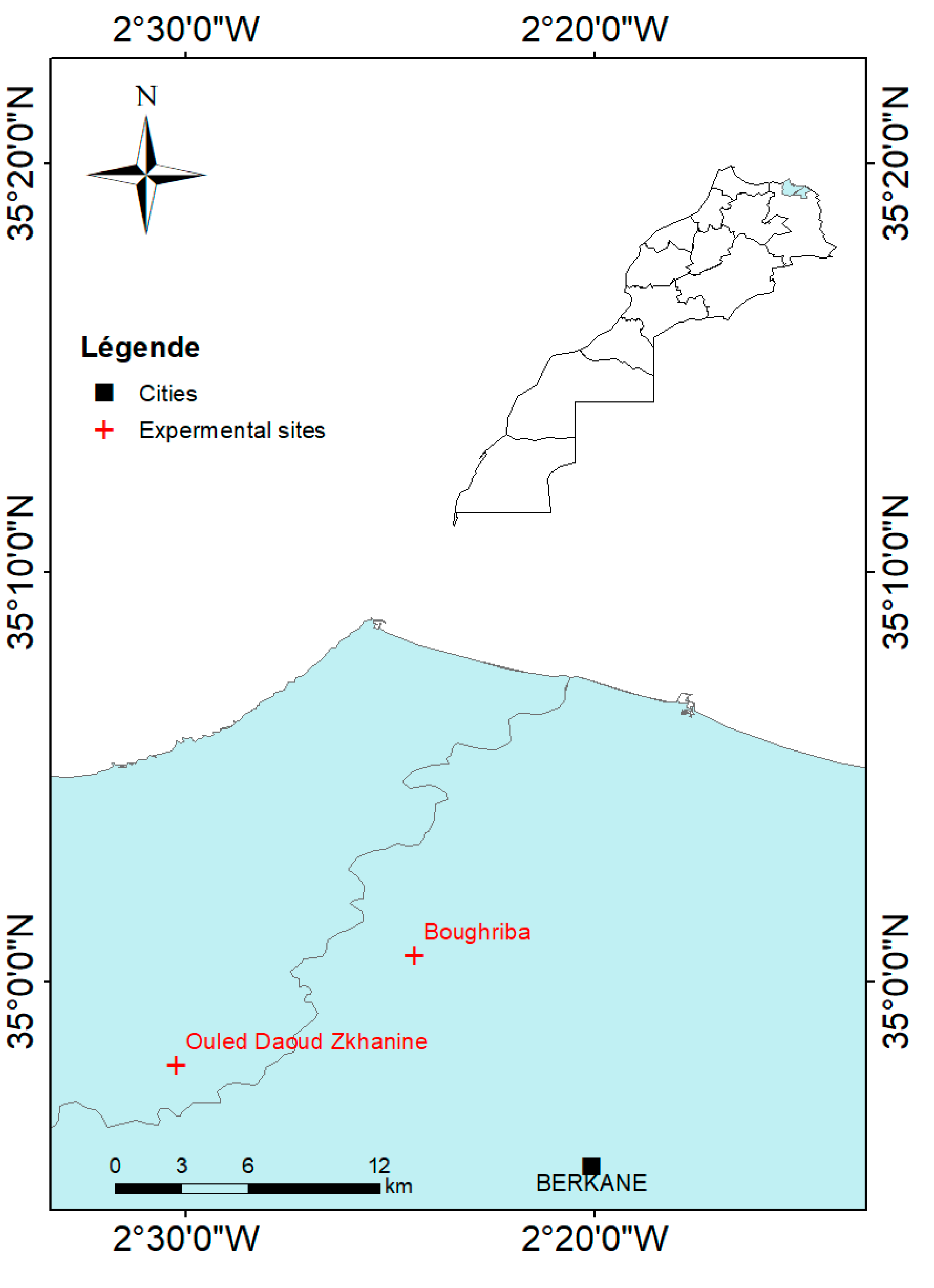
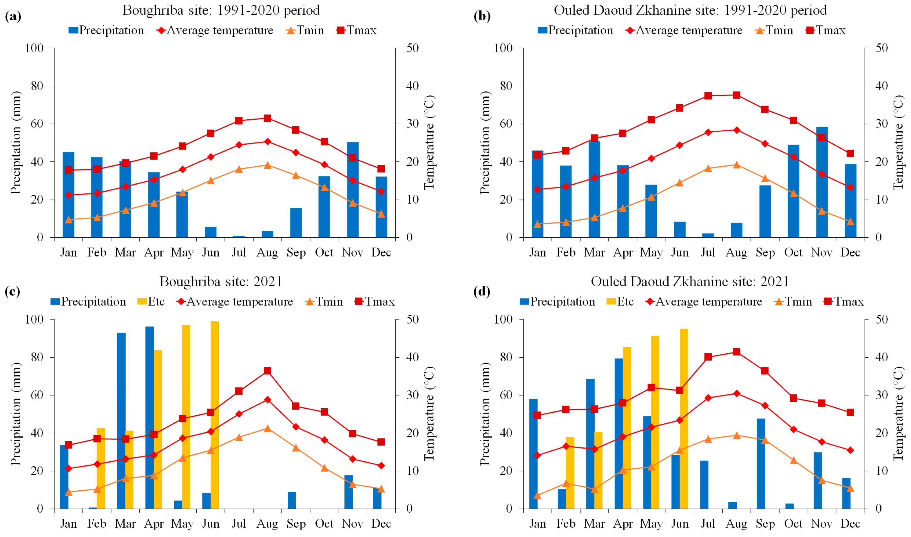
2.1. Experimental Sites

Field experiments were conducted in 2021 in two mature olive orchards in northeastern Morocco. The two sites are natural and organic farms, so no chemical products (pesticides and mineral fertilizers) were applied in accordance with the local practices. The first experimental site (S1) was situated within the Boughriba rural commune in Berkane Province (35°00′39″ N 2°24′23″ W, 52 m from sea level), while the second site (S2) (34°57′58″ N 2°30′12″ W, 62 m from sea level) was based in the Ouled Daoud Zkhanine rural commune in Nador Province (Figure 1).

Before starting the field experiment, soil analysis was performed at the laboratory of the National Institute for Agricultural Research in Rabat. The soil was silt loamy in S1 and loamy in S2. It contained 3.4 and 2.7% of organic matter, respectively. The soil in S2 is more highly rich in P, K, and NO₃ than S1. The other soil properties are reported in

Table 1. Soil properties at both experimental sites (0–30 cm).

	Boughriba Site (S1)		Ouled Daoud Zkhanine Site (S2)
	SCS	AFS	SCS	AFS
Texture	Silt loam	Silt loam	Loamy	Loamy
ECe (mS/cm, 25 °C)	1.25	1.38	2.45	2.40
OM (%)	3.13	3.59	2.53	2.85
PH	7.35	7.32	7.41	7.43
P2O5 (ppm)	3.25	4.90	32.45	35.15
K2O (ppm)	235	270	275	337
NO3 (ppm)	2.75	3.33	4.85	5.63
Ca (mg/100 g)	685	705	545	595
Mg (mg/100 g)	121	128	105	101
Active limestone (%)	8.24	8.75	7.95	8.68

AFS: agroforestry system; SCS: sole crop system. Soil analysis was performed at the laboratory of the National Institute for Agricultural Research in Rabat, Morocco.

.

In both experimental sites, the climate is typically semi-arid, characterized by sporadic annual rainfall. The average rainfall amounts over a 30-year period were 326.5 mm (CV = 29%) and 392.2 mm (CV = 24%) for S1 and S2, respectively. The average minimum and maximum temperatures were 11.3 and 23.7 °C (S1) and 10.2 and 29.4 °C (S2), respectively.

In 2021, the total rainfall was 273.3 mm and 419.5 mm in S1 and S2, respectively, while the corresponding values during the quinoa growing season (from February to June) were 202 mm and 261.3 mm. Compared to the long-term averages, we recorded increases of 27% and 37% regarding the cumulated rainfall during the quinoa growing season, respectively, for S1 and S2. The mean air temperatures were 17.3 and 18.9 °C in S1 and S2. The corresponding absolute maximum temperatures were 25.4 °C (June) and 32.1 °C (May), while the absolute minimum temperatures were 5.20 °C (February) and 5.21 °C (March), respectively.

As depicted by Figure 2a,b, S1 and S2 experienced drought from May to October and from May to September, respectively. Nevertheless, these diagrams exhibit drier plant establishment stages (February) during the quinoa growing season, indicating a reduction in rainfall of 98.6% (S1) and 72.2% (S2) compared to the same period’s long-term average (Figure 2c,d). Additionally, the quinoa growing season in S1 experienced a highly uneven distribution of rainfall, with only 0.3% in February, 93.6% in March and April, and 6% in May and June, while in S2, quinoa received 4%, 56.6%, and 29.7% of the total rainfall during the same periods. According to our study, the three periods correspond to the following stages: germination–emergence, panicle emergence–flowering, and grain filling–maturity. Moreover, the crop water requirements (ETc) emphasize the drought situation through the first and the latest stages of the quinoa growing season (Figure 2c,d).

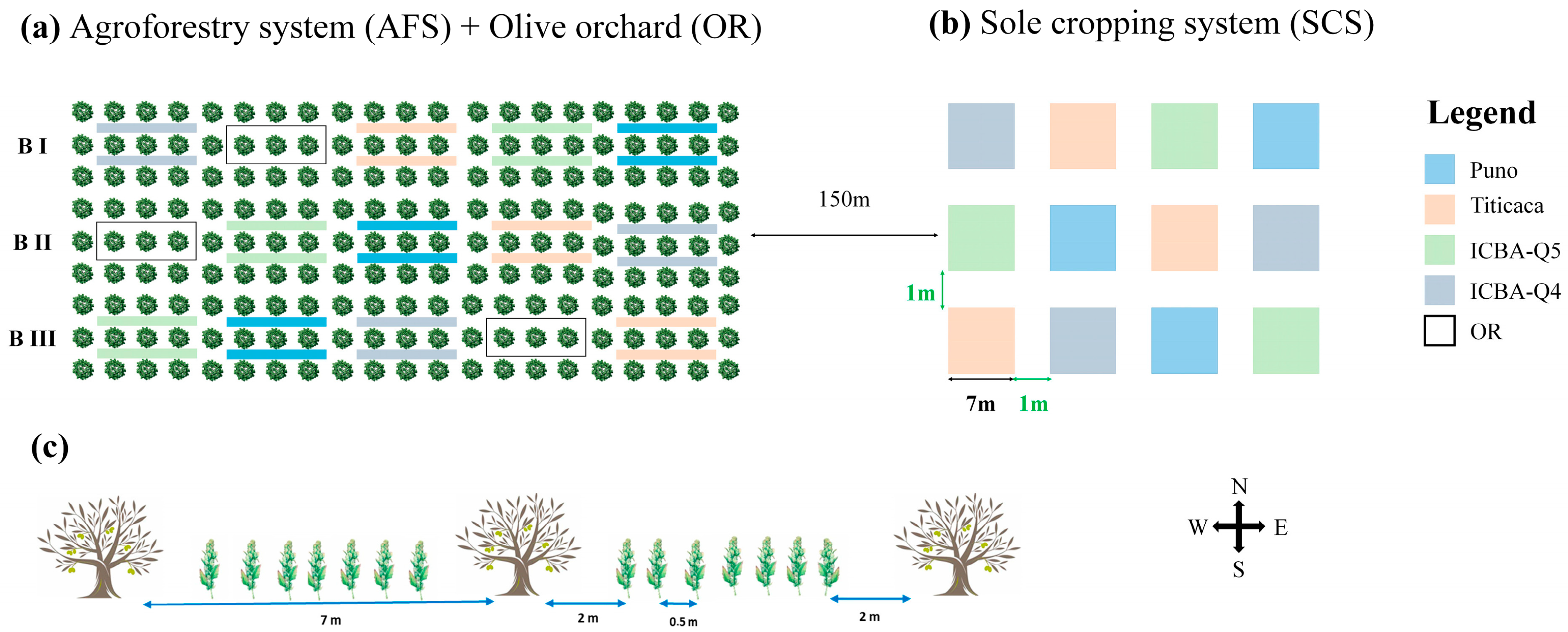
2.2. Plant Material and Experimental Setup

The olive grove (Olea europea, subsp europaea, cv. Picholine marocaine) was 57 and 52 years old in 2021 in S1 and S2, respectively. The density of olive trees at both locations was 200 trees ha⁻¹ with a regular 7 m × 7 m plantation design. Before the experiments, inter-rows were left uncultivated, and the olive trees rarely received gravity-fed irrigation to complement the rainfall supply.

The tested quinoa cultivars (Puno, Titicaca, ICBA-Q5, and ICBA-Q4) are characterized by short growing cycles (90 to 120 days), good performance, and large-scale adaptation under semi-arid conditions in Morocco [36,37,38].

For both experimental sites, the quinoa cultivars were intercropped with olive trees following the same experimental layout. The agroforestry system and the control orchard were in the same olive grove, while the sole quinoa cultivars were sown in an adjacent plot 150 m apart to avoid any interaction between trees and sole quinoa systems. Both agroforestry and sole cropping systems followed a randomized complete block design with 3 replications. For the agroforestry system, quinoa varieties were sown on either side of the middle olive tree row in the unit plot (Figure 3). The total area of the olive grove was 2940 m², divided into 15 plots of 196 m² each (14 m × 14 m). The agroforestry systems (AFS) used 12 of these plots, while the control orchard (OR) occupied 3 plots. The quinoa rows were oriented east–west, parallel to the olive tree rows. Similarly, 12 plots of 49 m² (7 m × 7 m) each were assigned to the sole crop system (SCS), covering a total area of 590 m².

In both AFS and SCS, quinoa varieties were manually sown with an inter-row and intraplant spacing of 0.5 m and 0.25 m, respectively. Within the AFS, 2 m was maintained between the olive trees and quinoa. Quinoa in S1 was sown on 18 February and harvested on 3 July, while in S2, the sowing and harvesting dates were 20 February and 5 July, respectively. As our experiments were conducted on organic (S1) and natural (S2) farms, local organic manure (10 t ha⁻¹) was supplied, and weeds were manually managed.

To secure grain germination and emergence under drought conditions that prevailed at the onset of the quinoa growing cycle (February) in both experimental sites, supplemental irrigation (SI) was exclusively applied during this period through a drip irrigation system. The drip lines were spaced apart by 0.5 m, with 2 l h⁻¹ integral drippers spaced 0.3 m apart. The total irrigation added during February amounted to 42 mm and 28 mm, respectively, for S1 and S2. The crop water requirement was estimated based on the Formula (1).

$${ET}_C=k_C\times {ET}_0$$

(1)

where k_c is the crop coefficient: 0.5 at plant establishment and 1 during flowering and seed fillings [39].

ET₀ was calculated using the Penman–Monteith formula [40] based on climatic parameters collected from local meteorological stations.

2.3. Field Measurments and Sampling

At quinoa flowering, 10 plants were randomly selected on each side of the central row of olive trees, avoiding the borders to assess the plant height. Measurements were performed out from the ground level to the top of quinoa panicle of the mean stem [41].

At quinoa maturity, in each plot, an area of 2 m² was randomly selected on either side of the median row of olive trees, avoiding the borders. Afterward, quinoa plants were threshed, sorted by organ, oven-dried (70 °C, 48 h), and weighted to determine the total aboveground biomass, the grain yield, and the thousand-kernel weight. The harvest index was calculated as the ratio between the grain yield and total aboveground biomass. For the sole crop system (SCS), we evaluated all the monitored parameters in a 2 m² area within each plot.

To measure the olive yield per tree, we randomly selected 3 trees in the middle of each plot to avoid border effects. Then, olives were manually harvested and weighted.

2.4. Quinoa Water Productivity (QWP) and Land Equivalent Ratio (LER)

Quinoa water productivity was calculated as the ratio between the obtained quinoa yield and the amount of supplied water, including the irrigation applied to ensure the quinoa’s emergence. To assess land use efficiency, we evaluated the land equivalent ratio (LER) as the relative land area required for sole crops and trees to achieve the same total yield as agroforestry [42]. LER was calculated as the sum of relative yields in agroforestry compared to the sole crop and the orchard tree yields (Formulas (2)–(4)).

$${LER}_{AFS}={LER}_{Olive}+{LER}_{Quinoa}$$

(2)

$${LER}_{Olive}=\frac{{Olive yield}_{AFS}}{{Olive yield}_{OR}}$$

(3)

$${LER}_{Quinoa}=\frac{{Quinoa yield}_{AFS}}{{Quinoa yield}_{SCS}}$$

(4)

The LER indicates higher (or lower) productivity for an agroforestry system (AFS) than the corresponding orchard (OR) and sole crop (SCS) when its value is above (or below) 1. When this value is equal to 1, the agroforestry system has no significant impact on land productivity [6].

2.5. Quinoa Seed Analysis

2.5.1. Grain Protein, Gross Cellulose, and Mineral Contents

The analysis of chemical and biochemical parameters was performed at the laboratory of the National Institute of Agronomic Research (INRA) in Rabat. The seed’s protein content was calculated using Formula (5), considering that most proteins contain 16% nitrogen [43].

$$Protein (\% dry matter)=N content \left(\% dry matter\right)\times 6.25$$

(5)

where nitrogen was analyzed according to the Kjeldal method. The fat and cellulose contents were determined using a Soxhlet extractor and Weende method (Weende, 1993), respectively. Regarding the grain mineral content analysis, we used the protocol as described by [44]. The mineral matter was determined after the calcination of the dry samples at 550 °C.

2.5.2. Extraction of Bioactive Components

Saponins were extracted following the method of [45] with slight modifications. Briefly, 5 g of each quinoa seed’s powder was placed in a filter paper cartridge and defatted using the Soxhlet apparatus with hexane (1:10 w/v) as a solvent. Ultrasound-assisted extraction of saponins was performed with methanol (1:10 w/v). Extraction was carried out using an ultrasonic probe at 60% amplitude for 15 min (3 cycles of 5 min). The mixture was filtered through Whatman paper N°1. The mixture was centrifuged, and the supernatant was dried under vacuum and then reconstituted in 5 mL of methanol.

2.5.3. Total Saponin Content

The modified technique described by [46] was employed to determine the overall saponin content. In this procedure, 0.25 mL of the saponin extract was combined with 1 mL of a reagent mixture (comprising glacial acetic acid and sulfuric acid in a 1:1 v/v ratio) and subjected to vortexing. Subsequently, the mixture underwent incubation at 60 °C in a water bath for 30 min, followed by cooling in an ice bath. A UV–visible spectrophotometer (VWR International, Radnor, PA, USA) was utilized to measure the absorbance of the sample at 527 nm. Calibration curve preparation involved using oleanolic acid within the concentration range of 0 to 1000 μg/mL. The expression of the total saponin content was in grams of oleanolic acid equivalent per 100 g of dry weight (DW).

2.5.4. Total Phenolic Content (TPC)

The determination of the total phenolic content followed the procedure outlined by [47]. Each sample, consisting of 200 mL aliquots, was combined with 1 mL of 10% Folin reagent and allowed to stand in the dark at room temperature for 6 min. Subsequently, 800 mL of 7.5% Na₂CO₃ (w/v) was introduced into the mixture, and the reaction proceeded in the dark for 30 min before we measured optical densities at 750 nm. A control was also prepared, and the calibration curve utilized gallic acid as the reference standard. The expression of the total phenolic content was in milligrams of gallic acid equivalent (GAE) per 100 g of dry weight (DW).

2.5.5. Antioxidant Activity (AOX)

The assessment of the scavenging activity of quinoa extract was performed using the 2,2-diphenyl-2-picryl-hydrazyl (DPPH) assay, following the protocol outlined by [48]. In summary, 4.9 mL of a 0.1 mM methanolic DPPH solution (violet color) was combined with 100 μL of varying concentrations of quinoa extract. The reaction occurred in the dark at room temperature for 30 min, and the reduction in violet color intensity was gauged at 517 nm. A positive control, substituting methanol for the sample, was prepared, and a standard curve was established using Trolox (0–12 µmole). The outcomes are presented in micromoles of Trolox per gram of extract (µmol TE/g E).

2.6. Statistical Analysis

Statistical analyses were performed using the R programming language (R Core Team, Vienna, Austria, 2021). The additive model of the analysis of variance (ANOVA) was used to assess the effects of three factors (experimental site, cropping system, and quinoa variety) on the monitored parameters (agronomic and biochemical parameters). The comparison of means was performed using the Student–Newman–Keuls test at p < 0.05. Pearson’s correlation matrix was performed to investigate the strength of the linear relationship between the investigated parameters, with values ranging from −1 (perfect negative correlation) to 1 (perfect positive correlation) and 0 (no linear correlation). The matrix graphical representation was carried out using the corrplot package. In addition, principal component analysis (PCA) was utilized to examine the correlation between the traits and evaluate the impact of the factors on the identified correlation patterns. To perform the PCA, the “FactomineR” and “Factoextra” packages were used, and the factors were projected as supplementary qualitative variables.

3. Results

3.1. Grain Yield and Yield-Related Components

The highly significant effects of the cropping system, experimental site, quinoa cultivars, and their interactions on grain yield are reported in

Table 2. Grain yield and yield-related components as affected by the monitored factors and their interactions.

		Plant Height (cm)		Grain Yield (t ha−1)		Dry Biomass (t ha−1)		HI		TKW (g)		Quinoa Water Productivity (kg m−3)
F	Site	6.5 *		42.2 ***		69.2 ***		7.0 *		432.1 ***		14.8 ***
	CS	9.2 **		100.2 ***		153 ***		12.4 **		1.8 ns		94.7 ***
	Variety	3.1 *		6.8 **		9.5 ***		1.3 ns		16.2 ***		6.3 **
	Site × CS	4.6 *		23.1 ***		36.5 ***		1.1 ns		2.6 ns		16.5 ***
	Site × Variety	0.5 ns		11.0 ***		12.6 ***		2.0 ns		5.8 **		10.6 ***
	CS × Variety	1.6 ns		10.9 ***		11.7 ***		1.3 ns		8.0 ***		10.5 ***
	Site × CS × Variety	1.7 ns		10.7 ***		11.1 ***		0.3 ns		1.8 ns		10.4 ***
Sites	Varieties	AFS	SCS	AFS	SCS	AFS	SCS	AFS	SCS	AFS	SCS	AFS	SCS
Site 1	Puno	111.7 ± 5.8 a	97.3 ± 3.1 a	1.1 ± 0.2 a	1 ± 0.2 b	2.4 ± 0.4 a	2.3 ± 0.6 b	0.5 ± 0 a	0.4 ± 0 a	2.5 ± 0.1 ab	2.5 ± 0.1 b	0.6 ± 0.1 a	0.5 ± 0.1 b
	Titicaca	111.0 ± 14.9 a	114 ± 16.5 a	0.9 ± 0.1 a	1 ± 0.2 b	2 ± 0.3 a	2.4 ± 0.4 b	0.4 ± 0 a	0.4 ± 0.1 a	2.6 ± 0 a	2.7 ± 0 a	0.4 ± 0.1 a	0.5 ± 0.1 b
	ICBa-Q5	124.7 ± 19.4 a	125 ± 27.8 a	0.9 ± 0.0 a	2.1 ± 0.4 a	2.2 ± 0.3 a	5.3 ± 1.1 a	0.4 ± 0 a	0.4 ± 0 a	2.4 ± 0.1 b	2.1 ± 0.1 d	0.5 ± 0 a	1.1 ± 0.2 a
	ICBAQ4	121.3 ± 7.2 a	117.7 ± 15.4 a	0.8 ± 0.1 a	1.4 ± 0.4 b	1.9 ± 0.2 a	3.2 ± 0.6 b	0.4 ± 0 a	0.4 ± 0.1 a	2.6 ± 0 a	2.3 ± 0.1 c	0.4 ± 0.1 a	0.7 ± 0.2 b
Means		117.2 ± 12.8 A	113.5 ± 18.6 A	0.9 ± 0.17 B	1.4 ± 0.56 A	2.1 ± 0.34 B	3.3 ± 1.38 A	0.44 ± 0.03 A	0.42 ± 0.04 A	2.5 ± 0.12 A	2.4 ± 0.22 B	0.5 ± 0.09 B	0.7 ± 0.28 A
Site 2	Puno	101.0 ± 18.2 a	88.3 ± 10.4 a	1.2 ± 0.2 a	1.7 ± 0.5 b	2.5 ± 0.4 a	4.3 ± 0.8 b	0.5 ± 0.0 a	0.4 ± 0 a	3.4 ± 0.0 a	3.4 ± 0.3 a	0.5 ± 0.1 a	0.7 ± 0.2 b
	Titicaca	108.0 ± 22.6 a	109.3 ± 18.5 a	1.1 ± 0.1 a	3.5 ± 0.3 a	2.6 ± 0.5 a	8.7 ± 0.7 a	0.4 ± 0.0 a	0.4 ± 0 a	3.0 ± 0.1 c	3.3 ± 0.2 a	0.5 ± 0 a	1.5 ± 0.1 a
	ICBa-Q5	128.3 ± 20.2 a	85.0 ± 13.2 a	1.0 ± 0.1 a	2.4 ± 0.4 b	2.4 ± 0.3 a	6.1 ± 1.0 b	0.4 ± 0.0 a	0.4 ± 0 a	3.1 ± 0.1 bc	2.9 ± 0.1 a	0.4 ± 0 a	1.0 ± 0.2 b
	ICBAQ4	124.7 ± 5.0 a	93.3 ± 5.8 a	1.1 ± 0.2 a	1.7 ± 0.4 b	2.7 ± 0.5 a	4.6 ± 1.1 b	0.4 ± 0.0 a	0.4 ± 0 a	3.3 ± 0.1 ab	3.2 ± 0.2 a	0.5 ± 0.1 a	0.7 ± 0.2 b
Means		115.5 ± 19.3 A	94 ± 14.7 B	1.1 ± 0.14 B	2.3 ± 0.87 A	2.5 ± 0.37 B	5.9 ± 1.97 A	0.43 ± 0.03 A	0.39 ± 0.03 B	3.2 ± 0.18 A	3.2 ± 0.28 A	0.5 ± 0.06 B	1 ± 0.37 A
Overall means		116.3 ± 16.0 A	103.8 ± 19.2 B	1.0 ± 0.17 B	1.9 ± 0.86 A	2.3 ± 0.41 B	4.6 ± 2.13 A	0.44 ± 0.03 A	0.4 ± 0.04 B	2.9 ± 0.12 A	2.8 ± 0.22 A	0.47 ± 0.07 B	0.83 ± 0.35 A

Values are means ± standard deviation (n = 12). For each site and each cropping system, means followed by the same lowercase letters are not significantly different. For each parameter, means followed by the same uppercase letters are not significantly different. *, **, *** indicate the significance level at p < 0.05, 0.01, and 0.001, respectively. AFS and SCS are agroforestry and sole cropping systems, respectively. The statistical analysis was performed using R programming language.

. Overall, the grain yield was higher in SCS than AFS (1.9 t ha⁻¹ vs. 1 t/ha, p < 0.001). This significant increase was more pronounced in S2 (+53%) than in S1 (+35%), with the highest grain yields provided by Titicaca in S2 (3.5 t ha⁻¹) and ICBA-Q5 in S1 (2.1 t ha⁻¹) when grown in SCS. In AFS, no significant differences were recorded among the quinoa varieties at either location. The average grain yields were 1.15 and 1.7 t ha⁻¹ for S1 and S2, respectively.

The variation in dry matter followed the same trends as grain yield, being significantly lower in AFS compared to SCS (2.3 t ha⁻¹ vs. 4.6 t ha⁻¹, p < 0.001). This significant decline was more substantial in S2 (−57%) than S1 (−37%), highlighting the significant effect of the interaction between cropping system and experimental site (p < 0.001) (Table 2). Moreover, this parameter was on average 55.6% higher in S2 than S1. The average dry matters were 2.7 and 4.2 t ha⁻¹ for S1 and S2, respectively. Furthermore, significant differences were noticed among the quinoa cultivars when grown as sole crops in S1 and S2, with the highest values recorded by ICBA-Q5 (5.3 t ha⁻¹) and Titicaca (8.7 t ha⁻¹), respectively. On the other hand, no significant changes were recorded among the quinoa varieties in AFS (Table 2).

Conversely to grain yield and dry matter, the harvest index (HI) showed no significant variation among the quinoa cultivars, and there were no significant interactions between the three factors (Table 2). Significant variance for HI was reported within cropping systems in S2 (p < 0.01) and through experimental sites (p < 0.05).

The quinoa genetic variability (p < 0.01) and the specific conditions at the experimental sites (p < 0.05) were the main factors influencing the thousand-kernel weight individually, while there was no significant difference between the two cropping systems (Table 2). On the other hand, significant interactions were recorded between experimental site and quinoa varieties and between cropping system and quinoa varieties. This parameter was 30% higher in S2 compared to S1. On average, the lowest 1000-kernel weight (2.6 g) was exhibited by ICBA-Q5.

As Table 2 exhibits, plant height at the flowering stage significantly varied according to the cropping system (p ≤ 0.01). Indeed, this parameter was 12% higher within the AFS than the SCS. Simultaneously, the average of plant height differed significantly between S1 and S2 (115.35 cm vs. 104.75 cm, p ≤ 0.05) and among quinoa varieties (p ≤ 0.05), with the highest average exhibited by ICBA-Q5 (115.8 cm). Furthermore, a significant interaction between the cropping system and the experimental site (p ≤ 0.05) was recorded, with an increase of 23% in the AFS in S2. However, no significant effects were observed among quinoa cultivars when grown as sole crops in the same experimental site.

3.2. Quinoa Water Productivity (QWP)

Quinoa water productivity was significantly affected by the local conditions of the experimental sites (p < 0.001), cropping systems (p < 0.001), quinoa cultivars (p < 0.01), and their interactions (p < 0.001). This parameter was 44% higher in SCS than that expected from AFS, and 25% higher in S2 than S1. The highest averages were, respectively, recorded at S2 (0.75 5 kg m⁻³), with SCS (0.8 5 kg m⁻³), and with Titicaca (0.73 5 kg m⁻³) and ICBA-Q5 (0.74 5 kg m⁻³). Moreover, the quinoa cultivars exhibited greater water productivity in SCS than AFS. Unlike Puno in S1, the highest quinoa water productivity was achieved by ICBA-Q5 (1.1 5 kg m⁻³) in S1 and Titicaca (1.5 kg m⁻³) in S2 (Table 2).

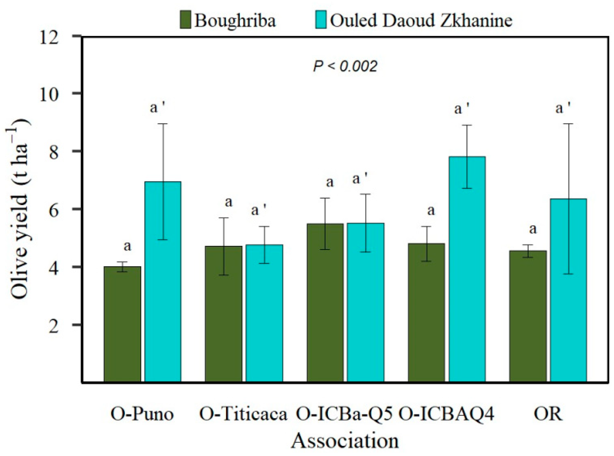
3.3. Olive Yield Comparison between Agroforestry Systems (O-AFS) and Olive Orchard

The olive yield was significantly higher in S2 than S1 (6.26 t ha⁻¹ vs. 4.77 t ha⁻¹, p < 0.01). Moreover, the comparison between olive yields in the AFS and orchard showed no significant difference. The highest yields were recorded for ICBA-Q5 in S1 and ICBA-Q4 in S2 (Figure 4).

3.4. Land Equivalent Ratio (LER)

To assess the contribution of quinoa varieties and olive trees to the total productivity of the agroforestry system, the partial land equivalent ratios of quinoa varieties (LER_Quinoa) and olive trees (LER_Olive) were calculated. The average LER_Quinoa ranged from 0.45 to 0.99, indicating that the quinoa component contributed between 45% and 99% of the total productivity, respectively, depending on the quinoa variety–olive tree association. Similarly, LER_Olive averaged from 0.93 to 1.19, showing that olive trees contributed between 93% and 119% of the total productivity. As depicted in

Table 3. Partial and combined land equivalent ratios as affected by quinoa varieties and experimental site conditions.

Sites	Associations	LERQuinoa	LEROlive	LER
Mean	O-Puno	0.99 ± 0.41 a	1.08 ± 0.48 a	2.07 ± 0.54 a
	O-Titicaca	0.60 ± 0.34 b	0.93 ± 0.26 a	1.54 ± 0.52 b
	O-ICBA-Q5	0.45 ± 0.09 b	1.06 ± 0.22 a	1.51 ± 0.23 b
	O-ICBA-Q4	0.66 ± 0.23 b	1.19 ± 0.29 a	1.85 ± 0.27 ab
F	Site	8.36 *	0.17 ns	3.16 ns
	Variety	5.74 **	0.93 ns	4.23 *
	Site × Variety	3.18 ns	2.40 ns	3.08 ns

Values are means ± standard deviation (n = 6). For each parameter, means followed by the same letters are not significantly different. * and ** indicate the significance level at p < 0.05 and 0.01, respectively. The statistical analysis was performed using R programming language.

, the combined land equivalent ratio (LER) exceeded 1 for all associations, averaging from 1.51 to 2.07, indicating that the productivity was 51% to 107% higher in AFS than SCS. In addition, the results revealed no significant variance in the LER between the two sites, whereas this parameter significantly varied among the four olive–quinoa cultivar associations depending on the quinoa variety (p < 0.05). Considering the partial land equivalent ratios, LER_Quinoa varied significantly depending on the experimental site (p < 0.05) and quinoa variety (p < 0.01), unlike LER_Olive.

3.5. Variation in Protein, Fat, and Cellulose Content in Quinoa Seeds

The grain protein content in AFS was significantly higher than in SCS, with a slight difference of 4% (p < 0.001). Moreover, this parameter was 5% higher in S1 than S2. The grain protein content significantly varied among the quinoa cultivars (p < 0.001) when intercropped with olive trees in both experimental sites and when grown as sole crops in S1. However, this parameter was similar among all varieties grown as sole crops under the environmental conditions in S2 (

Table 4. Variation in grain protein, fat, and cellulose contents at harvest according to cropping systems, experimental sites, and quinoa varieties.

		Protein (% DM)		Fat (% DM)		Cellulose (% DM)
F	Site	61.2 ***		120.9 ***		3 ns
	CS	38.9 ***		0 ns		0.1 ns
	Variety	7.8 ***		6.6 **		2.9 ns
	Site × CS	5.6 *		0.1 ns		1 ns
	Site × Variety	3.9 *		5.3 **		1.2 ns
	CS × Variety	1.5 ns		7.2 ***		2.7 ns
	Site × CS × Variety	0.2 ns		5.8 **		6.4 **
Sites	Varieties	AFS	SCS	AFS	SCS	AFS	SCS
Site 1	Puno	16 ± 0.1 ab	15.5 ± 0.2 ab	4.9 ± 0.1 ab	4.8 ± 0 a	7.3 ± 0.2 a	7.4 ± 0.1 b
	Titicaca	16.2 ± 0.2 a	16 ± 0.2 a	5.1 ± 0.1 a	5.1 ± 0.2 a	7 ± 0.1 a	7.2 ± 0.1 b
	ICBa-Q5	16.1 ± 0.2 a	15.9 ± 0.3 a	4.6 ± 0.2 b	4.8 ± 0.2 a	7.3 ± 0.4 a	7.9 ± 0.1 a
	ICBAQ4	15.7 ± 0.1 b	15.2 ± 0.3 b	4.7 ± 0.2 ab	4.7 ± 0.2 a	7.2 ± 0.3 a	6.7 ± 0.4 c
Means		16 ± 0.2 A	15.7 ± 0.4 B	4.8 ± 0.2 A	4.9 ± 0.2 A	7.2 ± 0.3 A	7.3 ± 0.5 A
Site 2	Puno	15.4 ± 0.1 ab	14.3 ± 0.9 a	7.9 ± 1.8 a	6.8 ± 0.1 b	6.7 ± 0.4 b	7.1 ± 0.8 a
	Titicaca	15.8 ± 0.1 a	15.4 ± 0.4 a	5.7 ± 0.4 b	7.7 ± 0.5 a	6.8 ± 0 b	7.2 ± 0.6 a
	ICBa-Q5	15.2 ± 0.1 b	14.6 ± 0.2 a	5.2 ± 0.1 b	6 ± 0 c	7.9 ± 0.1 a	6.6 ± 0 a
	ICBAQ4	15.7 ± 0.3 ab	14.6 ± 0.1 a	8.1 ± 1.6 a	6.3 ± 0.2 c	7.1 ± 0.2 b	7 ± 0.9 a
Means		15.5 ± 0.3 A	14.7 ± 0.6 B	6.7 ± 1.7 A	6.7 ± 0.7 A	7.1 ± 0.5 A	7 ± 0.6 A
Overall means		15.8 ± 0.4 A	15.2 ± 0.7 B	5.8 ± 1.5 A	5.8 ± 1.1 A	7.2 ± 0.26 A	7.1 ± 0.49 A

Values are means ± standard deviation (n = 12). For each site and cropping system, means followed by the same lowercase letters are not significantly different. For each parameter, means followed by the same uppercase letters are not significantly different. *, **, *** indicate the significance level at p < 0.05, 0.01, and 0.001, respectively. AFS: agroforestry system. SCS: sole cropping system. Chemical analyses were performed at the laboratory of the National Institute for Agricultural Research in Rabat Morocco. The statistical analysis was carried out using R programming language.

). Significant interactions between the experimental sites, quinoa cultivars, and cropping systems were also reported (p < 0.001), with values ranging from 15.2% to 16.2% and from 14.3% to 16% in AFS and in SCS, respectively. Titicaca recorded the best average grain protein content (15.8%) (Table 4).

Table 4 shows the significant effects on grain fat content in S1 and S2 (4.85% cv 6.7%, p < 0.001) and between all quinoa cultivars (p < 0.01), averaging from 5.1% ICBA-Q5 to 6.1% (Puno). Nevertheless, the cropping system did not significantly affect the grain fat content. Significant interactions between the studied factors were also observed. Regarding grain cellulose content, Table 4 exhibits no significant differences between either site, either system, and the quinoa varieties. Nevertheless, cellulose content was significantly affected by the interactions between the three factors (p < 0.05).

3.6. Variation in Mineral Content in Quinoa Seeds

As depicted in

Table 5. Variation in mineral content in quinoa seeds at harvest.

		P (mg kg−1 DM)		K (mg kg−1 DM)		Ca (mg kg−1 DM)		Fe (mg kg−1 DM)		Na (mg kg−1 DM)
F	Site	0 ns		1.1 ns		57.2 ***		18.1 ***		0.1 ns
	CS	16.7 ***		4.7 *		0.3 ns		0.1 ns		3.8 ns
	Variety	23.2 ***		3.3 *		3 *		5.6 **		5 **
	Site × CS	5.3 *		13.9 ***		0.2 ns		3.6 ns		1.6 ns
	Site × Variety	22.9 ***		8.9 ***		3.4 *		0.6 ns		3.9 *
	CS × Variety	17.5 ***		0.6 ns		1.6 ns		0.7 ns		2.4 ns
	Site × CS × Variety	82.8 ***		1.2 ns		0.2 ns		4.1 *		0.6 ns
Sites	Varieties	AFS	SCS	AFS	SCS	AFS	SCS	AFS	SCS	AFS	SCS
Site 1	Puno	354.9 ± 1.8 b	353.1 ± 2.8 b	971.8 ± 4.8 a	4SQZ3	147.6 ± 1.3 a	148.4 ± 1 a	16.9 ± 0.1 a	15.5 ± 0.5 b	4.2 ± 0.1 a	4.1 ± 0 a
	Titicaca	375.3 ± 4.5 a	322.1 ± 0.2 c	938.6 ± 6 a	933.7 ± 1.4 b	149.9 ± 1.1 a	149.3 ± 1 a	15.6 ± 1.3 a	15.6 ± 0.6 b	4.1 ± 0.1 a	4.7 ± 0.1 a
	ICBa-Q5	359.2 ± 2.4 b	355.4 ± 10 b	977.1 ± 6.3 a	953.9 ± 1.5 a	150.1 ± 1.7 a	149.6 ± 0.7 a	15.9 ± 0.6 a	15.3 ± 0.4 b	4.6 ± 0.3 a	4.8 ± 0.4 a
	ICBAQ4	355.1 ± 0.1 b	367.9 ± 2.2 a	957.9 ± 27.7 a	914.9 ± 6.1 c	150.1 ± 1.9 a	149.4 ± 0.6 a	16.2 ± 0.4 a	16.9 ± 0.1 a	4.4 ± 0.4 a	4.5 ± 0.2 a
Means		361.1 ± 9 A	349.6 ± 18.2 B	961.3 ± 20 A	935.6 ± 14.9 B	149.4 ± 1.7 A	149.2 ± 0.9 A	16.2 ± 0.8 A	15.8 ± 0.8 A	4.3 ± 0.3 A	4.5 ± 0.3 A
Site 2	Puno	388.8 ± 0.6 a	363.3 ± 4.4 a	944.6 ± 40.2 a	948.3 ± 3 b	147 ± 0.2 b	147.8 ± 0.2 a	15.1 ± 0.7 a	15.7 ± 0.4 a	4.4 ± 0.2 a	4.2 ± 0.2 a
	Titicaca	315.8 ± 0.7 d	366.6 ± 10.2 a	930.9 ± 21.1 a	934.4 ± 0.8 b	147.4 ± 0.3 ab	146.6 ± 0.6 b	15.1 ± 0.4 a	15.5 ± 0.6 a	4.3 ± 0.1 a	4.5 ± 0.4 a
	ICBa-Q5	383.7 ± 0.2 b	338.2 ± 16 a	926.7 ± 0.6 a	935.4 ± 2.1 b	147 ± 0.1 b	147.4 ± 0.1 a	14.7 ± 0.4 a	15.2 ± 0.6 a	4.3 ± 0.2 a	4.3 ± 0.3 a
	ICBAQ4	339.6 ± 4.6 c	346.9 ± 8.3 a	959.5 ± 16.9 a	970.9 ± 16.5 a	147.9 ± 0.2 a	147.5 ± 0.5 a	15.8 ± 0.4 a	15.5 ± 0.2 a	4.6 ± 0 a	4.8 ± 0.1 a
Means		357.0 ± 31.9 A	353.8 ± 15.2 A	940.4 ± 24.6 A	947.2 ± 17 A	147.3 ± 0.4 A	147.3 ± 0.6 A	15.2 ± 0.6 A	15.5 ± 0.5 A	4.4 ± 0.2 A	4.4 ± 0.3 A
Overall means		359.0 ± 23.0 A	351.7 ± 16.5 B	950.9 ± 24.4 A	941.4 ± 16.7 B	148.4 ± 1.6 A	148.2 ± 1.2 A	15.7 ± 0.9 A	15.6 ± 0.6 A	4.4 ± 0.3 A	4.5 ± 0.3 A

Values are means ± standard deviation (n = 12). For each site and cropping system, means followed by the same lowercase letters are not significantly different. For each parameter and each site, means followed by the same uppercase letters are not significantly different. *, **, *** indicate the significance level at p < 0.05, 0.01, and 0.001, respectively. AFS: agroforestry system. SCS: sole cropping system. Chemical analyses were performed at the laboratory of the National Institute for Agricultural Research in Rabat Morocco. The statistical analysis of Puno and ICBA-Q5 was carried out using R programming language. With regard to the effect of the experimental site, no significant variances in DPPH were observed.

, the results revealed that the cropping system significantly affected the phosphorus and potassium contents, which were slightly higher in agroforestry than in sole crops (3%). However, sodium, iron, and calcium were not affected by the cropping system. Additionally, the local conditions of the experimental sites significantly influenced grain calcium and iron contents (p < 0.001), unlike phosphorus and potassium. Significant differences in all grain mineral contents were reported considering the quinoa genotype effect. Puno recorded the highest values with regard to P and K seed contents (365 mg/100 g DW vs. 951 mg/100 g DW), whereas ICBA-Q4 averaged the highest values of Ca and iron seed contents (148 mg/100 g DW vs. 16.1 mg/100 g DW).

3.7. Saponin, Total Polyphenol (TPC), and DPPH Contents in Seeds

Saponins are a class of chemical compounds found in a broad spectrum of plant species including quinoa chenopodium and are known for their characteristic bitter taste.

Table 6. Seed quinoa contents of saponin, TPC, and DPPH.

		Saponin (% DM−1)		TPC (mg GAE/100 g DM)		DPPH (µmol TE/g E)
F	Site	7.2 *		2.6 ns		0.02 ns
	CS	9.6 **		5.7 *		5.6 *
	Variety	6.8 **		8.1 ***		21.8 ***
	Site × CS	22.3 ***		0.7 ns		0.6 ns
	Site ×Variety	2.5 ns		1.3 ns		3.7 *
	CS × Variety	30.4 ***		2.9 ns		4.3 *
	Site × CS × Variety	3.2 *		1.6 ns		2.7 ns
Sites	Varieties	AFS	SCS	AFS	SCS	AFS	SCS
Site 1	Puno	0.3 ± 0.1 bc	0.3 ± 0 a	891.7 ± 2.5 a	832.5 ± 7.1 b	40.7 ± 0.4 a	31.8 ± 0.7 a
	Titicaca	0.2 ± 0.1 c	0.2 ± 0 b	801.4 ± 1.7 a	598.3 ± 2.7 c	33 ± 0.5 b	31.7 ± 0.6 a
	ICBa-Q5	0.7 ± 0.1 a	0.1 ± 0 c	743.8 ± 128.9 a	449.3 ± 6.2 d	24.7 ± 0.7 b	23.7 ± 0.5 b
	ICBAQ4	0.4 ± 0 b	0.1 ± 0 c	778.5 ± 91.7 a	898 ± 1.8 a	28 ± 7.2 b	24.9 ± 0.4 b
Means		0.4 ± 0.2 A	0.2 ± 0.1 B	803.9 ± 88.4 A	694.5 ± 188.2 B	31.6 ± 7 A	28 ± 3.9 B
Site 2	Puno	0.4 ± 0.1 b	0.5 ± 0.2 a	845.4 ± 68.6 a	738.7 ± 160.3 a	39.7 ± 5.7 a	36.3 ± 6.1 a
	Titicaca	0.2 ± 0 b	0.4 ± 0.1 a	694.7 ± 25.1 a	545.6 ± 221.1 a	29.8 ± 6.8 ab	23.1 ± 5.5 a
	ICBa-Q5	0.5 ± 0 a	0.2 ± 0 a	648.8 ± 0 a	654.3 ± 233.4 a	19.8 ± 0.8 b	29.2 ± 3.8 a
	ICBAQ4	0.3 ± 0.1 b	0.5 ± 0.1 a	696.1 ± 170 a	738.9 ± 156.3 a	34.2 ± 3.8 a	27.7 ± 2.6 a
Means		0.3 ± 0.1 A	0.4 ± 0.2 A	721.2 ± 110.6 A	669.4 ± 186.5 A	30.9 ± 8.7 A	29.1 ± 6.3 A
Overall means		0.4 ± 0.18 A	0.3 ± 0.16 B	763 ± 107 A	682 ± 184 B	31.2 ± 7.7 A	28.5 ± 5.2 B

Values are means ± standard deviation (n = 12). For each site and cropping system, means followed by the same lowercase letters are not significantly different. For each parameter, means followed by the same uppercase letters are not significantly different. *, **, *** indicate the significance level at p < 0.05, 0.01, and 0.001, respectively. Chemical analyses were performed at the laboratory of the National Institute for Agricultural Research in Rabat Morocco. The statistical analysis was carried out using R programming language.

depicts significant differences in saponin content depending on the cropping system, quinoa cultivar, and their interactions under two different soil and climate conditions. The average ranged from 0.2% DM to 0.4%. Additionally, a significant increase in saponin content was shown in AFS (26%, p < 0.01). This increase was most pronounced in S1 (96%, p < 0.001). Furthermore, this parameter significantly varied between the experimental sites (0.3% in S1 vs. 0.36% in S2, p < 0.05). In AFS, the highest seed saponin contents were achieved by ICBA-Q5 (0.7% in S1 vs. 0.5% in S2).

Polyphenols are a large group of naturally occurring compounds that are known for their antioxidant properties and are found in a wide variety of plants. Their amount significantly varied depending on the quinoa genotype (p < 0.001) and cropping system (p < 0.05). In average, the highest and the lowest values of polyphenol content were recorded by Puno (827 mg GAE/100 g of DM) and by ICBA-Q5 (624 mg GAE/100 g of DM), respectively (Table 6). Likewise, the average polyphenol content was 12% and significantly higher in AFS than SCS with 16% in S1 (p < 0.001) vs. 8% in S2 (p = 0.434). However, no significant variation in this parameter was reported for experimental locations and interactions between the three factors.

Under abiotic stresses, quinoa produces various enzymatic and non-enzymatic antioxidants that work to scavenge reactive oxygen species (ROS). In our experiment, we used DPPH (2.2-diphenyl-2-picryl-hydrazyl) to evaluate the antioxidant activity. As depicted in Table 6, DPPH followed the same trends as TPC regarding the individual effects of the monitored factors. Significant variances in DPPH were observed depending on the cropping system (p < 0.05) and quinoa genotype (p < 0.001). DPPH was 9% higher in AFS than SCS; moreover, the highest and the lowest values averaged 37.1 and 24.4 µmol TE/g E, respectively.

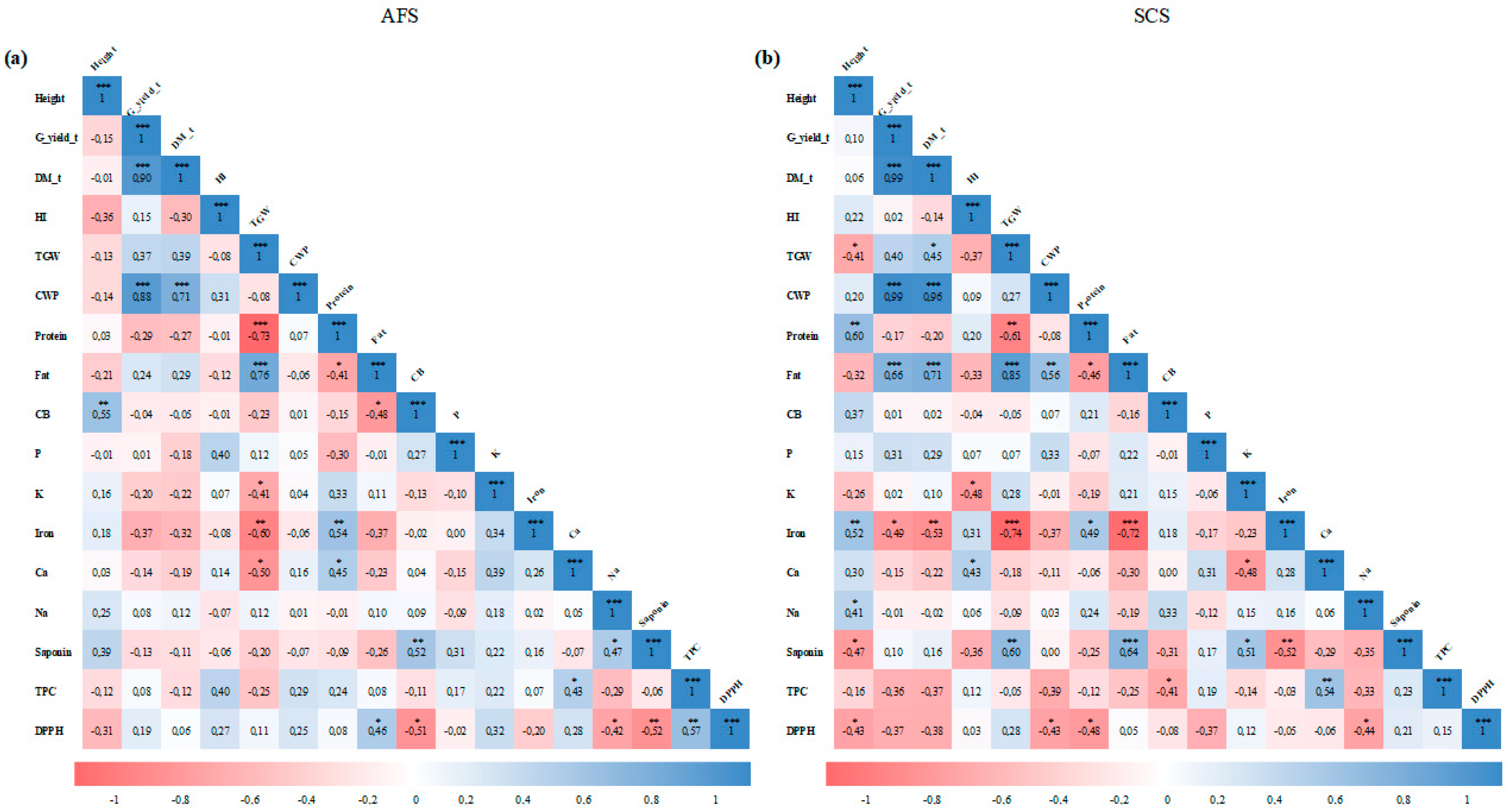
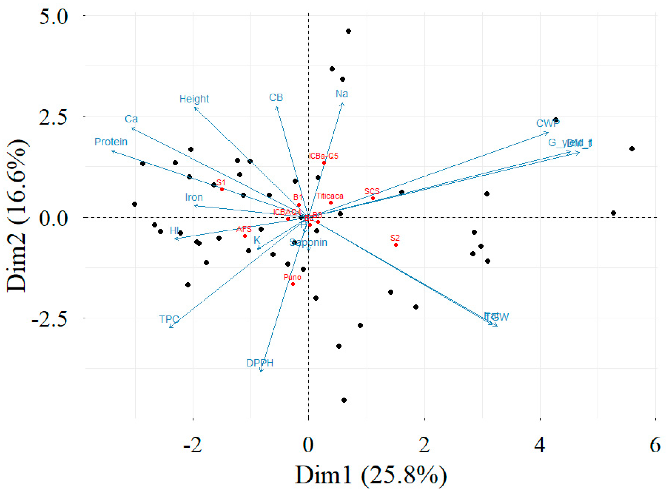
3.8. Correlation Matrix and Principal Component Analysis

In examining the relationships among the evaluated quinoa parameters, our findings revealed more significant correlations in SCS than in AFS (Figure 5). Indeed, quinoa grain yield, dry matter, water productivity, and seed contents of Fe, saponin, and fat were significantly correlated with more parameters in SCS than in AFS. For instance, in AFS, the grain yield was only correlated with the dry matter (r = 0.90) and crop water productivity (r = 0.88). However, in SCS, the grain yield was correlated with the dry matter (r = 0.99), crop water productivity (r = 0.99), and seed contents of fat (r = 0.66) and Fe (r = −0.49). In addition, for AFS, the seed fat content was only correlated with its contents of protein (r = −0.41), cellulose (r = −0.48), and DPPH (r = 0.45) and the 1000-kernel weight (r = 0.76). On the other hand, in SCS, the seed fat content was correlated with the grain yield (r = 0.66), dry matter (r = 0.71), crop water productivity (r = 0.56), and the seed contents of protein (r = −0.46), Fe (r = −0.72), and saponin (r = 0.64).

The results of PCA indicated that the first plane explained 42.3% of the data variability (Figure 6). This variability is significant since it is greater than the reference value of 26.6 [49]. Grain yield, dry matter, quinoa water productivity, thousand-kernel weight, and seed contents of protein and fat mostly contributed to the construction of the first dimension of the PCA. Grain yield, dry matter, TKW, and fat content were positively correlated with the first dimension of the PCA. Concerning the second component, it was mainly explained by DPPH, Na, CB, TPC, plant height, and the thousand-kernel weight. TPC, DPPH, iron, and HI were positively correlated with the second dimension of the PCA. However, plant height, Na, saponin, and CB were negatively correlated with the second dimension of the PCA. Moreover, the first plane of the PCA contrasted with the experimental sites and the cropping systems.

4. Discussion

In agroforestry, the interactions between trees and crops differently affect their growth and productivity, depending on the competition or facilitation for resources such as light, water, and nutrients. In Morocco, olive-based agroforestry is a promising way to sustain land management and to improve agricultural productivity thanks to its high adaptation to semi-arid conditions. Yet, under severe abiotic stresses, the yields of intercropped staple crops like cereals and legumes deleteriously decrease [23]. Thus, under such conditions, selecting appropriate and suitable tree–crop combinations is a priority. That is why, for the first time, we proposed to intercrop quinoa cultivars with olive trees. To test our hypothesis that this new intercropping system could be a sustainable agroecological option in semi-arid areas, we assessed yields, yield-related attributes, crop water productivity, land equivalent ratio, grain nutritional quality, and antioxidant parameters.

4.1. Yields and Yield-Related Components

The results showed that all investigated parameters were variously affected by cropping systems, soil and climate conditions, and quinoa genetic variability, as well as their interactions. Plant height was 12% and 23% significantly higher within the AFS and local conditions in S2, respectively. Conversely, grain yield and dry matter were 45% and 49% significantly lower in AFS compared to SCS. Likewise, these losses were more pronounced under the local conditions in S2 than in S1 (grain yield: −53% vs. −31%; dry matter: −57% vs. −35%). These results corroborate the finding of [22] on durum wheat and faba bean in olive-based agroforestry, [26] on legumes intercropped with olive trees, and [50] on wheat in poplar-based agroforestry. Similarly, [51] reported that apricot- and walnut-based intercropping systems negatively affected wheat grain yield, [52] found that dry matter production at the flowering stage of barley, durum wheat, and chickpea was significantly lower in AFS than SCS, and [25] indicated a marked reduction in the wheat grain yield in AFS (−43%) with regard to the shading level.

Considering the effects of local conditions, the rain was better distributed during the growing season of quinoa in S2 than S1, except at the beginning when we irrigated at both sites to ensure quinoa germination and emergence. In addition, the soil texture and its initial content of N, P, and K was richer in S2. These conditions probably improved the height in AFS, especially in S2, while the yield and dry matter were severely reduced in AFS and in S2. This outcome can be explained by the fact that the shading caused by olive trees was the most limiting factor of quinoa productivity, especially in S2, where the well-distributed rain was more profitable to olive trees and thereby increased the negative effect of shade on the quinoa. This is probably explained by the adaptation of quinoa to light stress by increasing its vegetation height and the severe losses of yield and dry biomass in AFS under S2. This result is aligned with the finding of [53] that shade might negatively affect crop productivity under wetter and colder conditions. In addition, the quinoa growing cycle corresponds to the period of full olive development and consequently confronts quinoa with competition from olive trees for nutrient and light interception. This result is in line with the authors of [51,54], who found that competition for light represents the main limiting factor for grain yield. Other findings [20,51] stipulated that negative linear correlations were observed between tree shade intensity and grain yield-related traits, but moderate shade was not a major limiting factor for barley yield in AFS. Furthermore, in our trials, the olive tree densities were higher than recommended in agroforestry (below 200 trees ha⁻¹) [55]. Similar findings were reported in Brazil by [56] where, when intercropping cacao with orange or avocado, trees reduced the cacao yield and plant vigor, especially when the planting distance was small. In addition, the distance between quinoa and trees (2 m) was not sufficient to avoid shade induced by an olive tree canopy.

The non-significant variance in TKW among both cropping systems as well as its increase in S2 (30%) relative to S1 confirms that the drought timing was the main factor determining the TKW during the seed filling stage. In fact, the drought occurred during May–June in S1, and the soil silt loamy texture reduced nutrient uptake and negatively affected the TKW, whereas shade in S2 enhanced this parameter by reducing evapotranspiration and increasing photosynthesis accumulation and nutrient uptake. This result corroborates the findings of [25] that the TKW and harvest index (HI) were slightly higher under moderate shade (AF; +12% vs. CS). Other research [22,51] reported that strong negative linear correlations were observed between tree shade intensity, wheat grain yield-related traits, and seed nutrient content (N, P and K).

The magnitude of grain yield and dry matter reduction depends on the quinoa genetic competitivity. In our experiments, ICBA-Q5 achieved the highest averages of these parameters, highlighting its higher tolerance to shade. However, its lower TKW was probably related to its high sensitivity to drought occurring during the grain filling stage in S1. Shade seemed not to have a significant effect on the number of grains, which probably offset the loss of grain yield. Similar compensation was reported in [22], where it was found that the loss of grain wheat in olive-based agroforestry was compensated by the increase in the total grain number.

4.2. Crop Water Productivity (CWP) and Land Equivalent Ratio (LER)

On average, crop water productivity was significantly (44%) lower in AFS than SCS, and this loss was more pronounced in S2 (−53%) than S1 (−31%). These results were explained by losses in grain yields and dry matter that occurred in AFS due to the shade, which was most intense in S2 and due to the drought at the filling stage in S1. Indeed, CWP was strongly and positively correlated with grain yield and dry matter in AFS (r = 0.88 vs. r = 0.71) and in SCS (r = 0.99 vs. r = 0.96). Additionally, the silt loamy texture in S1, making the soil less friable under the drought that occurred during the grain filling stage, limited the quinoa water and nutrient uptake, explaining the reduction in the grain yield observed in S1. In [57], it was reported that the seed-filling stage is the most sensitive growth stage of quinoa to drought stress.

The most recognized benefit of AFS lies in its potential to enhance land productivity by using resources more efficiently than SCS. In fact, in most cases, AFS predicted a favorable LER compared to sole crops and tree orchards. In our experiment, despite the low grain yields, AFS had higher land productivity than sole stands and tree orchards. LER was always greater than 1 and ranged from 1.57 (AFSO-ICBA-Q5) to 2.07 (AFSO-Puno), indicating that the productivity was 57% to 107% higher in AFS than SCS. Similar findings were reported by [5,22,26,58,59] when growing other annual crops within fruit tree-based agroforestry.

The olive yield average did not significantly vary between olive orchards and when associated with quinoa varieties. However, it was significantly higher in S2 than S1 (6.26 t ha⁻¹ vs. 4.77 t ha⁻¹, p < 0.01). This inter-location variability is likely due to different local conditions, including climate and soil fertility, since the olive-related traits (age: 57 vs. 52, density: 200 tree/ha, variety: Moroccan Picholine) were similar in both sites. Contrarily, the partial land equivalent ratios (LEROlive) were almost all greater than one, confirming that olive–quinoa associations were profitable for olive trees. This result may be explained by a complementarity interaction between olive trees and quinoa varieties, probably due to quinoa’s high potential to regulate soil salinity. In fact, quinoa is a facultative halophyte showing a more efficient control mechanism on xylem Na⁺ loading and better K⁺ retention, ensuring a higher K⁺/Na⁺ ratio [60] compared to staple crops. On the other hand, LER_Quinoa was always lower than 1, reflecting the competition between quinoa and olive trees in light interception, particularly in S2. Concerning water and nutrient uptake, quinoa probably only uses surface layers according to [61], who reported that water from surface layers could be used by annual crops without affecting the production of perennial crops.

4.3. Seed Nutritional Quality

Quinoa has exceptional nutritional properties including high mineral and protein contents, fat, and dietary fiber. Despite its broad adaptation to different environments, the variation in its nutritional components strongly depends on genetic variability, soil, and climate conditions, as well as their interactions [31]. In our experiment, the microclimate created by olive trees systematically and differently influenced the seed nutritional status of four quinoa varieties in both experimental sites.

The cropping system, quinoa cultivar, soil and climate conditions of the experimental sites, and their interactions factored in the determination of the protein, fat, cellulose, and mineral contents. For instance, AFS enhanced the protein content of quinoa seeds by 4%. This parameter was also 5% higher under the local conditions of S2 than S1 and varied significantly among quinoa varieties, with the highest average attained by Puno (15.8%). High values of fat and cellulose contents were also recorded by Puno (6.1% DW) and ICBA-Q5 (7.4% DW), respectively. Phosphorus and potassium varied significantly with quinoa variety, cropping system, and their interactions, while calcium, iron, and sodium depended essentially on soil and climate conditions. Additionally, P and K were significantly enhanced by AFS in S1. This result is probably explained by the fact that P and K were initially limited in S1, leading to more exploration of deeper layers by olive trees to make available these nutrients to the quinoa’s roots. Significant variations in both protein and amino acid contents were observed in [62] through six quinoa varieties cultivated under different pedoclimatic conditions. Similar findings were reported by [22] on wheat in olive-based agroforestry (4%), [63] on wheat in jujube- and walnut-based agroforestry, and [64] on soybean under Aonla trees. In [25,51], positive correlations between shade and protein content were reported.

The trees in AFS likely improved the soil structure and soil nutrient pools due to the high organic matter level resulting from the decomposition process of green biomass by soil microbial activity. Furthermore, the soil in S2 was initially richer in phosphorus, potassium, and nitrogen than in S1. The olive trees limited evapotranspiration and moderated the temperature by shading but also facilitated water and nutrient uptake due to their exploration in deeper layers, especially in S1. According to [18], water is distributed by trees’ roots from deep and wet soil layers to the upper and dry ones. This process, called “Hydraulic Lift (HL)” or water redistribution by roots, happens when there is a difference in soil water potential [65]. Through this mechanism, crops can take advantage of the soil nutrient pool to produce rich grains under water scarcity conditions in agroforestry systems [66]. In fact, mature olive trees may also provide more stability and structure to the system.

4.4. Saponin, Total Polyphenol, and DPPH Contents in Seeds

Besides their strong agronomic and nutritional properties related to their high adaptation to different environments and exceptional nutritional seed properties, quinoa seeds are rich in phytochemical components, such as phenolic compounds and saponins. These components may have beneficial effects on human health, such as antioxidant and anti-inflammatory properties.

Saponins are considered anti-nutritional secondary metabolites of the glycoside family, naturally produced by plants as a response to surrounding abiotic stress [67]. Quinoa seeds contain a high amount of saponins, which are mainly concentrated in the seed’s pericarp (86%) [68] and are responsible for the bitter or sweet taste [69]. The limit established to classify quinoa varieties as sweet or bitter is 0.11% saponin per seed fresh weight [70]. A myriad of environmental factors, such as water availability, salinity level, soil fertility, shading intensity, and genetic variability, are the main determinants of seeds’ saponin quantity and quality. In our experiment, seeds’ saponin content varied with regard to the cropping system, quinoa cultivar, soil, and climate conditions as well as their interactions. In AFS, an increase in this parameter was recorded and was strongly significant in S1 (96%), whereas, in S2, this parameter was slightly lower in AFS (10%). This result contradicts the outcomes of [71], which showed significantly lower contents of total saponins when applying different intensities of shading (70 and 90%) on P. polyphylla. In our case, the increase in saponin content in S1 is probably explained by the drought that occurred particularly during the filling stage or the interactions between shading induced by the olive trees. In this sense, [72,73] indicated that plants accumulate more saponins in response to abiotic stresses. Furthermore, in AFS, the highest seed saponin contents were achieved by ICBA-Q5 (0.7% in S1 vs. 0.5% in S2). These significant differences are in line with the finding of [74,75], where it was noted that saponin content is essentially considered a genotypic-dependent trait, even though it varies with abiotic stresses like drought and salinity.

Phenolic acids are also phytochemical compounds classified as secondary metabolites and are generated naturally by plants in response to stress (oxidative stress, salt stress, and drought stress) [76]. In our study, the total polyphenols in quinoa seeds significantly varied with quinoa genotype (p < 0.001) and cropping system (p < 0.05), averaging from 624 to 827 mg GAE/100 g DW for ICBA-Q5 and Puno, respectively. On average, the TPC was not significantly influenced by the experimental site; however, it was 16% higher in AFS than SCS under S1. S1 was characterized by limiting environmental conditions (sporadic rainfall with only 6% during the filling stage, and a silt loamy texture with lower soil amounts of P, K, and N). This result is also in agreement with previous authors who reported that saponins and TPC are systematically produced in response to unfavorable environmental conditions.

Under abiotic stresses (drought, shading, salinity…), quinoa produces various enzymatic and non-enzymatic antioxidants that work to scavenge reactive oxygen species (ROS). The mechanism consists of transferring electrons from antioxidants to free radicals to stabilize them. In our study, we evaluated the antioxidant capacity of plant extracts using DPPH (2.2-diphenyl-2-picryl-hydrazyl). DPPH and TPC were positively correlated (r = 0.57%, p < 0.01). On average, DPPH ranged from 24.4 to 37.1 mg/100 g DW for ICBA-Q5 and Puno, respectively.

On average, saponin, TPC, and DPPH contents were 26%, 12%, and 9% higher in AFS than SCS, respectively. AFS often increases soil organic matter and microbial activity. This can enhance nutrient cycling and nutrient availability to crops, which may positively influence antioxidant capacity under abiotic stresses [77].

4.5. Correlation Matrix and Principal Components Analysis

The correlation analysis revealed complex links between the evaluated quinoa parameters. Although the grain yield was correlated with other biomass production parameters in both AFS and SCS, the results were different regarding the other parameters, especially for saponin, DPPH, and Fe contents. In addition, for SCS, the grain yield was also related to the grain fat and Fe contents. This study is, to our knowledge, the first to investigate the links between agronomic parameters, seed nutrients contents, and other quality and physiological parameters in AFS and SCS. However, such relationships were analyzed in other pedoclimatic conditions. A positive correlation between grain yield, dry matter, and crop water productivity has been reported [62,78]. This analysis revealed more significant positive correlations (55%) in AFS than in SCS (45%) between the monitored parameters. According to these results, we can emphasize the higher synergistic relationships between quinoa varieties and olive trees in an agroforestry system.

Concerning the PCA, the experiment location and the cropping system were the main factors that discriminated between the individuals (Figure 6). This means that S2 recorded a higher grain yield, dry biomass, crop water productivity, thousand-grain weight, and grain fat content compared to S1. Similarly, AFS had higher plant height and grain protein content, but lower grain yield, dry biomass, crop water productivity, and thousand-grain weight compared to SCS. Also, the PCA emphasized that the grain yield, dry biomass, crop water productivity, thousand-grain weight, and grain fat were higher in SCS under the S2 conditions.

5. Conclusions

Olive-based agroforestry, traditionally practiced under rainfed conditions in Morocco’s semi-arid regions, commonly involves intercropping with cereals and legumes. However, the effectiveness of this traditional agroforestry has deleteriously declined due to climate change, particularly in arid and salinity-affected lands. Addressing this challenge, our study pioneered the intercropping of quinoa with olive trees for the first time in northeastern Morocco, assessing its viability as an eco-resilient crop in such environments. Our research focused on the influence of microclimate created by olive trees on the agronomic and biochemical traits of quinoa. Additionally, we evaluated the overall performance of this novel olive-based agroforestry system, particularly through the lens of the land equivalent ratio (LER). The results revealed an LER greater than one, reflecting that a quinoa–olive-based agroforestry approach could be a promising practice to enhance land use efficiency, sustain biodiversity, improve ecosystem services, and support local farmers in vulnerable environments to adapt to and mitigate climate change impacts. Given the promising outcomes, this study lays the groundwork for considering this system as a potential agroecological solution in semi-arid areas amidst the ongoing climate crisis. However, further research is essential to validate these findings. For instance, future studies should explore the productivity of quinoa under different tree-based agroforestry systems such as those involving pomegranate and carob, which are prevalent in northeastern regions known for dry and salinity-affected conditions. The nitrogen fixation ability of carob could offer additional benefits for quinoa cultivation. Moreover, optimizing the sowing dates for quinoa could mitigate competition for water and nutrients, further enhancing the effectiveness of this agroforestry model.

References

1. Santoro, A.; Venturi, M.; Bertani, R.; Agnoletti, M. A Review of the Role of Forests and Agroforestry Systems in the FAO Globally Important Agricultural Heritage Systems (GIAHS) Programme. Forests 2020, 11, 860. [Google Scholar] [CrossRef]
2. Castle, S.E.; Miller, D.C.; Merten, N.; Ordonez, P.J.; Baylis, K. Evidence for the Impacts of Agroforestry on Ecosystem Services and Human Well-Being in High-Income Countries: A Systematic Map. Environ. Evid. 2022, 11, 10. [Google Scholar] [CrossRef]
3. Santos, P.Z.F.; Crouzeilles, R.; Sansevero, J.B.B. Can Agroforestry Systems Enhance Biodiversity and Ecosystem Service Provision in Agricultural Landscapes? A Meta-Analysis for the Brazilian Atlantic Forest. For. Ecol. Manag. 2019, 433, 140–145. [Google Scholar] [CrossRef]
4. Colmenares, O.M.; Brindis, R.C.; Verduzco, C.V.; Grajales, M.P.; Gómez, M.U. Horticultural Agroforestry Systems Recommended for Climate Change Adaptation: A Review. Agric. Rev. 2020, 41, 14–24. [Google Scholar] [CrossRef]
5. Lehmann, L.M.; Smith, J.; Westaway, S.; Pisanelli, A.; Russo, G.; Borek, R.; Sandor, M.; Gliga, A.; Smith, L.; Ghaley, B.B. Productivity and Economic Evaluation of Agroforestry Systems for Sustainable Production of Food and Non-Food Products. Sustainability 2020, 12, 5429. [Google Scholar] [CrossRef]
6. Sereke, F.; Graves, A.R.; Dux, D.; Palma, J.H.N.; Herzog, F. Innovative Agroecosystem Goods and Services: Key Profitability Drivers in Swiss Agroforestry. Agron. Sustain. Dev. 2015, 35, 759–770. [Google Scholar] [CrossRef]
7. Mbow, C.; Van Noordwijk, M.; Luedeling, E.; Neufeldt, H.; Minang, P.A.; Kowero, G. Agroforestry Solutions to Address Food Security and Climate Change Challenges in Africa. Curr. Opin. Environ. Sustain. 2014, 6, 61–67. [Google Scholar] [CrossRef]
8. Vaast, P.; Harmand, J.-M.; Rapidel, B.; Jagoret, P.; Deheuvels, O. Coffee and Cocoa Production in Agroforestry—A Climate-Smart Agriculture Model. In Climate Change and Agriculture Worldwide; Torquebiau, E., Ed.; Springer: Dordrecht, The Netherlands, 2016; pp. 209–224. ISBN 978-94-017-7462-8. [Google Scholar]
9. Saqib, M.; Akhtar, J.; Abbas, G.; Murtaza, G. Enhancing Food Security and Climate Change Resilience in Degraded Land Areas by Resilient Crops and Agroforestry. In Climate Change-Resilient Agriculture and Agroforestry: Ecosystem Services and Sustainability; Castro, P., Azul, A.M., Leal Filho, W., Azeiteiro, U.M., Eds.; Climate Change Management; Springer International Publishing: Cham, Switzerland, 2019; pp. 283–297. ISBN 978-3-319-75004-0. [Google Scholar]
10. Sileshi, G.W.; Dagar, J.C.; Nath, A.J.; Kuntashula, E. Agroforestry as a Climate-Smart Agriculture: Strategic Interventions, Current Practices and Policies. In Agroforestry for Sustainable Intensification of Agriculture in Asia and Africa; Dagar, J.C., Gupta, S.R., Sileshi, G.W., Eds.; Sustainability Sciences in Asia and Africa; Springer Nature: Singapore, 2023; pp. 589–640. ISBN 978-981-19460-2-8. [Google Scholar]
11. Jose, S. Agroforestry for Conserving and Enhancing Biodiversity. Agrofor. Syst. 2012, 85, 1–8. [Google Scholar] [CrossRef]
12. Ntawuruhunga, D.; Ngowi, E.E.; Mangi, H.O.; Salanga, R.J.; Shikuku, K.M. Climate-Smart Agroforestry Systems and Practices: A Systematic Review of What Works, What Doesn’t Work, and Why. For. Policy Econ. 2023, 150, 102937. [Google Scholar] [CrossRef]
13. Octavia, D.; Murniati; Suharti, S.; Hani, A.; Mindawati, N.; Suratman; Swestiani, D.; Junaedi, A.; Undaharta, N.K.E.; Santosa, P.B.; et al. Smart Agroforestry for Sustaining Soil Fertility and Community Livelihood. For. Sci. Technol. 2023, 19, 315–328. [Google Scholar] [CrossRef]
14. van Noordwijk, M.; Speelman, E.; Hofstede, G.J.; Farida, A.; Abdurrahim, A.Y.; Miccolis, A.; Hakim, A.L.; Wamucii, C.N.; Lagneaux, E.; Andreotti, F.; et al. Sustainable Agroforestry Landscape Management: Changing the Game. Land 2020, 9, 243. [Google Scholar] [CrossRef]
15. Murniati, M.; Suharti, S.; Yeny, I.; Minarningsih, M. Cacao-Based Agroforestry in Conservation Forest Area: Farmer Participation, Main Commodities and Its Contribution to the Local Production and Economy. For. Soc. 2022, 6, 243–274. [Google Scholar] [CrossRef]
16. Sollen-Norrlin, M.; Ghaley, B.B.; Rintoul, N.L.J. Agroforestry Benefits and Challenges for Adoption in Europe and Beyond. Sustainability 2020, 12, 7001. [Google Scholar] [CrossRef]
17. Isaac, M.E.; Borden, K.A. Nutrient Acquisition Strategies in Agroforestry Systems. Plant Soil 2019, 444, 1–19. [Google Scholar] [CrossRef]
18. Bayala, J.; Prieto, I. Water Acquisition, Sharing and Redistribution by Roots: Applications to Agroforestry Systems. Plant Soil 2020, 453, 17–28. [Google Scholar] [CrossRef]
19. Schroth, G.; Sinclair, F.L. Trees, Crops and Soil Fertility: Concepts and Research Methods. For. Sci. 2003, 51, 91. [Google Scholar]
20. Vaccaro, C.; Six, J.; Schöb, C. Moderate Shading Did Not Affect Barley Yield in Temperate Silvoarable Agroforestry Systems. Agrofor. Syst. 2022, 96, 799–810. [Google Scholar] [CrossRef]
21. Daoui, K.; Fatemi, Z.E.A. Agroforestry Systems in Morocco: The Case of Olive Tree and Annual Crops Association in Saïs Region. In Science, Policy and Politics of Modern Agricultural System: Global Context to Local Dynamics of Sustainable Agriculture; Behnassi, M., Shahid, S.A., Mintz-Habib, N., Eds.; Springer: Dordrecht, The Netherlands, 2014; pp. 281–289. ISBN 978-94-007-7957-0. [Google Scholar]
22. Temani, F.; Bouaziz, A.; Daoui, K.; Wery, J.; Barkaoui, K. Olive Agroforestry Can Improve Land Productivity Even under Low Water Availability in the South Mediterranean. Agric. Ecosyst. Environ. 2021, 307, 107234. [Google Scholar] [CrossRef]
23. Amassaghrou, A.; Bouaziz, A.; Daoui, K.; Belhouchette, H.; Ezzahouani, A.; Barkaoui, K. Productivité et efficience des systèmes agroforestiers à base d’oliviers au Maroc: Cas de Moulay Driss Zerhoun. Cah. Agric. 2021, 30, 2. [Google Scholar] [CrossRef]
24. Chehab, H.; Tekaya, M.; Ouhibi, M.; Gouiaa, M.; Zakhama, H.; Mahjoub, Z.; Laamari, S.; Sfina, H.; Chihaoui, B.; Boujnah, D.; et al. Effects of Compost, Olive Mill Wastewater and Legume Cover Cropson Soil Characteristics, Tree Performance and Oil Quality of Olive Trees Cv.Chemlali Grown under Organic Farming System. Sci. Hortic. 2019, 253, 163–171. [Google Scholar] [CrossRef]
25. Panozzo, A.; Huang, H.; Bernazeau, B.; Vamerali, T.; Samson, M.F.; Desclaux, D. Morphology, Phenology, Yield, and Quality of Durum Wheat Cultivated within Organic Olive Orchards of the Mediterranean Area. Agronomy 2020, 10, 1789. [Google Scholar] [CrossRef]
26. Amassaghrou, A.; Barkaoui, K.; Bouaziz, A.; Alaoui, S.B.; Fatemi, Z.E.A.; Daoui, K. Yield and Related Traits of Three Legume Crops Grown in Olive-Based Agroforestry under an Intense Drought in the South Mediterranean. Saudi J. Biol. Sci. 2023, 30, 103597. [Google Scholar] [CrossRef] [PubMed]
27. Aumeeruddy-Thomas, Y.; Moukhli, A.; Haouane, H.; Khadari, B. Ongoing Domestication and Diversification in Grafted Olive–Oleaster Agroecosystems in Northern Morocco. Reg. Environ. Chang. 2017, 17, 1315–1328. [Google Scholar] [CrossRef]
28. Zahour, M. Food Security in Morocco: Risk Factors and Governance. In Emerging Challenges to Food Production and Security in Asia, Middle East, and Africa: Climate Risks and Resource Scarcity; Behnassi, M., Barjees Baig, M., El Haiba, M., Reed, M.R., Eds.; Springer International Publishing: Cham, Switzerland, 2021; pp. 149–170. ISBN 978-3-030-72987-5. [Google Scholar]
29. Bazile, D.; Pulvento, C.; Verniau, A.; Al-Nusairi, M.S.; Ba, D.; Breidy, J.; Hassan, L.; Mohammed, M.I.; Mambetov, O.; Otambekova, M.; et al. Worldwide Evaluations of Quinoa: Preliminary Results from Post International Year of Quinoa FAO Projects in Nine Countries. Front. Plant Sci. 2016, 7, 850. [Google Scholar] [CrossRef] [PubMed]
30. Lavini, A.; Pulvento, C.; d’Andria, R.; Riccardi, M.; Choukr-Allah, R.; Belhabib, O.; Yazar, A.; İncekaya, Ç.; Metin Sezen, S.; Qadir, M.; et al. Quinoa’s Potential in the Mediterranean Region. J. Agron. Crop Sci. 2014, 200, 344–360. [Google Scholar] [CrossRef]
31. Matías, J.; Rodríguez, M.J.; Cruz, V.; Calvo, P.; Granado-Rodríguez, S.; Poza-Viejo, L.; Fernández-García, N.; Olmos, E.; Reguera, M. Assessment of the Changes in Seed Yield and Nutritional Quality of Quinoa Grown under Rainfed Mediterranean Environments. Front. Plant Sci. 2023, 14, 1268014. [Google Scholar] [CrossRef]
32. Saddiq, M.S.; Wang, X.; Iqbal, S.; Hafeez, M.B.; Khan, S.; Raza, A.; Iqbal, J.; Maqbool, M.M.; Fiaz, S.; Qazi, M.A.; et al. Effect of Water Stress on Grain Yield and Physiological Characters of Quinoa Genotypes. Agronomy 2021, 11, 1934. [Google Scholar] [CrossRef]
33. Bazile, D.; Bertero, H.; Nieto, C. State of the Art Report on Quinoa around the World in 2013; FAO & CIRAD: Santiago, Chile, 2015; 603p. [Google Scholar]
34. Rodríguez Gómez, M.J.; Matías Prieto, J.; Cruz Sobrado, V.; Calvo Magro, P. Nutritional Characterization of Six Quinoa (Chenopodium quinoa Willd) Varieties Cultivated in Southern Europe. J. Food Compos. Anal. 2021, 99, 103876. [Google Scholar] [CrossRef]
35. Olivera, L.; Best, I.; Paredes, P.; Perez, N.; Chong, L.; Marzano, A.; Olivera, L.; Best, I.; Paredes, P.; Perez, N.; et al. Nutritional Value, Methods for Extraction and Bioactive Compounds of Quinoa. In Pseudocereals; IntechOpen: London, UK, 2022; ISBN 978-1-80355-181-4. [Google Scholar]
36. Qureshi, A.S.; Daba, A.W. Evaluating Growth and Yield Parameters of Five Quinoa (Chenopodium quinoa W.) Genotypes under Different Salt Stress Conditions. J. Agric. Sci. 2020, 12, 128. [Google Scholar] [CrossRef]
37. Hirich, A.; Rafik, S.; Rahmani, M.; Fetouab, A.; Azaykou, F.; Filali, K.; Ahmadzai, H.; Jnaoui, Y.; Soulaimani, A.; Moussafir, M.; et al. Development of Quinoa Value Chain to Improve Food and Nutritional Security in Rural Communities in Rehamna, Morocco: Lessons Learned and Perspectives. Plants 2021, 10, 301. [Google Scholar] [CrossRef]
38. Abidi, I.; Hirich, A.; Bazile, D.; Mahyou, H.; Gaboun, F.; Alaoui, S.B. Using Agronomic Parameters to Rate Quinoa (Chenopodium quinoa Willd.) Cultivars Response to Saline Irrigation under Field Conditions in Eastern Morocco. Environ. Sci. Proc. 2022, 16, 67. [Google Scholar] [CrossRef]
39. Garcia, M.; Raes, D.; Jacobsen, S.-E. Evapotranspiration Analysis and Irrigation Requirements of Quinoa (Chenopodium quinoa) in the Bolivian Highlands. Agric. Water Manag. 2003, 60, 119–134. [Google Scholar] [CrossRef]
40. Allan, R.; Pereira, L.; Raes, D.; Smith, M. Crop Evapotranspiration—Guidelines for Computing Crop Water Requirements—FAO Irrigation and Drainage Paper 56; FAO: Rome, Italy, 1998; Volume 56. [Google Scholar]
41. Hussain, M.I.; Muscolo, A.; Ahmed, M.; Asghar, M.A.; Al-Dakheel, A.J. Agro-Morphological, Yield and Quality Traits and Interrelationship with Yield Stability in Quinoa (Chenopodium quinoa Willd.) Genotypes under Saline Marginal Environment. Plants 2020, 9, 1763. [Google Scholar] [CrossRef]
42. Mead, R.; Willey, R.W. The Concept of a ‘Land Equivalent Ratio’ and Advantages in Yields from Intercropping. Exp. Agric. 1980, 16, 217–228. [Google Scholar] [CrossRef]
43. Chang, S.K.C.; Zhang, Y. Protein Analysis. In Food Analysis; Nielsen, S.S., Ed.; Food Science Text Series; Springer International Publishing: Cham, Switzerland, 2017; pp. 315–331. ISBN 978-3-319-45776-5. [Google Scholar]
44. Pequerul, A.; Pérez, C.; Madero, P.; Val, J.; Monge, E. A Rapid Wet Digestion Method for Plant Analysis. In Optimization of Plant Nutrition: Refereed Papers from the Eighth International Colloquium for the Optimization of Plant Nutrition, 31 August–8 September 1992, Lisbon, Portugal; Fragoso, M.A.C., Van Beusichem, M.L., Houwers, A., Eds.; Developments in Plant and Soil Sciences; Springer: Dordrecht, The Netherlands, 1993; pp. 3–6. ISBN 978-94-017-2496-8. [Google Scholar]
45. Navarro del Hierro, J.; Herrera, T.; García-Risco, M.R.; Fornari, T.; Reglero, G.; Martin, D. Ultrasound-Assisted Extraction and Bioaccessibility of Saponins from Edible Seeds: Quinoa, Lentil, Fenugreek, Soybean and Lupin. Food Res. Int. 2018, 109, 440–447. [Google Scholar] [CrossRef]
46. Lim, J.G.; Park, H.-M.; Yoon, K.S. Analysis of Saponin Composition and Comparison of the Antioxidant Activity of Various Parts of the Quinoa Plant (Chenopodium quinoa Willd.). Food Sci. Nutr. 2020, 8, 694–702. [Google Scholar] [CrossRef]
47. Gómez-Caravaca, A.M.; Segura-Carretero, A.; Fernández-Gutiérrez, A.; Caboni, M.F. Simultaneous Determination of Phenolic Compounds and Saponins in Quinoa (Chenopodium quinoa Willd) by a Liquid Chromatography–Diode Array Detection–Electrospray Ionization–Time-of-Flight Mass Spectrometry Methodology. J. Agric. Food Chem. 2011, 59, 10815–10825. [Google Scholar] [CrossRef]
48. Fischer, S.; Wilckens, R.; Jara, J.; Aranda, M. Variation in Antioxidant Capacity of Quinoa (Chenopodium quinoa Will) Subjected to Drought Stress. Ind. Crops Prod. 2013, 46, 341–349. [Google Scholar] [CrossRef]
49. Husson, F.; Lê, S.; Pagès, J. Exploratory Multivariate Analysis by Example Using R, 2nd ed.; Chapman and Hall/CRC: New York, NY, USA, 2017; ISBN 978-0-429-22543-7. [Google Scholar]
50. Kumar, A.; Singh, V.; Shabnam, S.; Oraon, P.R.; Kumari, S. Comparative Study of Wheat Varieties under Open Farming and Poplar-Based Agroforestry System in Uttarakhand, India. Curr. Sci. 2019, 117, 1054. [Google Scholar] [CrossRef]
51. Qiao, X.; Sai, L.; Chen, X.; Xue, L.; Lei, J. Impact of Fruit-Tree Shade Intensity on the Growth, Yield, and Quality of Intercropped Wheat. PLoS ONE 2019, 14, e0203238. [Google Scholar] [CrossRef] [PubMed]
52. Ben Zineb, A.; Barkaoui, K.; Karray, F.; Mhiri, N.; Sayadi, S.; Mliki, A.; Gargouri, M. Olive Agroforestry Shapes Rhizosphere Microbiome Networks Associated with Annual Crops and Impacts the Biomass Production under Low-Rainfed Conditions. Front. Microbiol. 2022, 13, 977797. [Google Scholar] [CrossRef]
53. Jacobs, S.R.; Webber, H.; Niether, W.; Grahmann, K.; Lüttschwager, D.; Schwartz, C.; Breuer, L.; Bellingrath-Kimura, S.D. Modification of the Microclimate and Water Balance through the Integration of Trees into Temperate Cropping Systems. Agric. For. Meteorol. 2022, 323, 109065. [Google Scholar] [CrossRef]
54. Dufour, L.; Metay, A.; Talbot, G.; Dupraz, C. Assessing Light Competition for Cereal Production in Temperate Agroforestry Systems Using Experimentation and Crop Modelling. J. Agron. Crop Sci. 2013, 199, 217–227. [Google Scholar] [CrossRef]
55. Singh, G.; Mutha, S.; Bala, N. Effect of Tree Density on Productivity of a Prosopis Cineraria Agroforestry System in North Western India. J. Arid. Environ. 2007, 70, 152–163. [Google Scholar] [CrossRef]
56. Tadesse, S.; Gebretsadik, W.; Muthuri, C.; Derero, A.; Hadgu, K.; Said, H.; Dilla, A. Crop Productivity and Tree Growth in Intercropped Agroforestry Systems in Semi-Arid and Sub-Humid Regions of Ethiopia. Agrofor. Syst. 2021, 95, 487–498. [Google Scholar] [CrossRef]
57. Hirich, A.; Allah, R.C.; Jacobsen, S.; Youssfi, L.E.; Homaria, H.E. Using Deficit Irrigation with Treated Wastewater in the Production of Quinoa (Chenopodium quinoa Willd.) in Morocco. Rev. Cient. UDO Agrícola 2012, 12, 570–583. [Google Scholar]
58. Bai, W.; Sun, Z.; Zheng, J.; Du, G.; Feng, L.; Cai, Q.; Yang, N.; Feng, C.; Zhang, Z.; Evers, J.B.; et al. Mixing Trees and Crops Increases Land and Water Use Efficiencies in a Semi-Arid Area. Agric. Water Manag. 2016, 178, 281–290. [Google Scholar] [CrossRef]
59. Žalac, H.; Zebec, V.; Ivezić, V.; Herman, G. Land and Water Productivity in Intercropped Systems of Walnut—Buckwheat and Walnut–Barley: A Case Study. Sustainability 2022, 14, 6096. [Google Scholar] [CrossRef]
60. Hussin, S.A.; Ali, S.H.; Lotfy, M.E.; El-Samad, E.H.A.; Eid, M.A.; Abd-Elkader, A.M.; Eisa, S.S. Morpho-Physiological Mechanisms of Two Different Quinoa Ecotypes to Resist Salt Stress. BMC Plant Biol. 2023, 23, 374. [Google Scholar] [CrossRef]
61. Lövenstein, H.M.; Berliner, P.R.; van Keulen, H. Runoff Agroforestry in Arid Lands. For. Ecol. Manag. 1991, 45, 59–70. [Google Scholar] [CrossRef]
62. Granado-Rodríguez, S.; Aparicio, N.; Matías, J.; Pérez-Romero, L.F.; Maestro, I.; Gracés, I.; Pedroche, J.J.; Haros, C.M.; Fernandez-Garcia, N.; Navarro del Hierro, J.; et al. Studying the Impact of Different Field Environmental Conditions on Seed Quality of Quinoa: The Case of Three Different Years Changing Seed Nutritional Traits in Southern Europe. Front. Plant Sci. 2021, 12, 649132. [Google Scholar] [CrossRef]
63. Qiao, X.; Xiao, L.; Gao, Y.; Zhang, W.; Chen, X.; Sai, L.; Lei, J.; Xue, L.; Zhang, Y.; Li, A. Yield and Quality of Intercropped Wheat in Jujube- and Walnut-Based Agroforestry Systems in Southern Xinjiang Province, China. Agron. J. 2020, 112, 2676–2691. [Google Scholar] [CrossRef]
64. Sharma, A.; Sharma, K.; Thakur, M.; Kumar, S. Protein Content Enhanced in Soybean under Aonla-Based Agroforestry System. Agrofor. Syst. 2023, 97, 261–272. [Google Scholar] [CrossRef]
65. Richards, J.H.; Caldwell, M.M. Hydraulic Lift: Substantial Nocturnal Water Transport between Soil Layers by Artemisia Tridentata Roots. Oecologia 1987, 73, 486–489. [Google Scholar] [CrossRef] [PubMed]
66. Bogie, N.A.; Bayala, R.; Diedhiou, I.; Conklin, M.H.; Fogel, M.L.; Dick, R.P.; Ghezzehei, T.A. Hydraulic Redistribution by Native Sahelian Shrubs: Bioirrigation to Resist In-Season Drought. Front. Environ. Sci. 2018, 6, 98. [Google Scholar] [CrossRef]
67. Ashour, A.S.; El Aziz, M.M.A.; Gomha Melad, A.S. A Review on Saponins from Medicinal Plants: Chemistry, Isolation, and Determination. J. Nanomed. Res. 2019, 7, 282–288. [Google Scholar] [CrossRef]
68. Ando, H.; Chen, Y.-C.; Tang, H.; Shimizu, M.; Watanabe, K.; Mitsunaga, T. Food Components in Fractions of Quinoa Seed. Food Sci. Technol. Res. 2002, 8, 80–84. [Google Scholar] [CrossRef]
69. Suárez-Estrella, D.; Torri, L.; Pagani, M.A.; Marti, A. Quinoa Bitterness: Causes and Solutions for Improving Product Acceptability. J. Sci. Food Agric. 2018, 98, 4033–4041. [Google Scholar] [CrossRef]
70. Kozioł, M.J. Chemical Composition and Nutritional Evaluation of Quinoa (Chenopodium quinoa Willd.). J. Food Compos. Anal. 1992, 5, 35–68. [Google Scholar] [CrossRef]
71. Chen, W.; Liu, S.; Geng, D.; Gu, Y.; Li, Z.; Pan, J.; Bai, Y. Effect of shading on saponin content and biochemical indexes of Paris polyphylla Smith var. chinensis (Franch.) Hara in northern Zhejiang. Chin. J. Eco-Agric. 2022, 30, 72–81. [Google Scholar]
72. Ariyanti, N.A.; Latifa, S. Saponins Accumulation and Antimicrobial Activities on Shallot (Allium Cepa L.) from Marginal Land. J. AGRO 2021, 8, 188–198. [Google Scholar] [CrossRef] [PubMed]
73. Zang, Z.; Liang, J.; Yang, Q.; Zhou, N.; Li, N.; Liu, X.; Liu, Y.; Tan, S.; Chen, S.; Tang, Z. An Adaptive Abiotic Stresses Strategy to Improve Water Use Efficiency, Quality, and Economic Benefits of Panax Notoginseng: Deficit Irrigation Combined with Sodium Chloride. Agric. Water Manag. 2022, 274, 107923. [Google Scholar] [CrossRef]
74. Pandya, A.; Thiele, B.; Zurita-Silva, A.; Usadel, B.; Fiorani, F. Determination and Metabolite Profiling of Mixtures of Triterpenoid Saponins from Seeds of Chilean Quinoa (Chenopodium quinoa) Germplasm. Agronomy 2021, 11, 1867. [Google Scholar] [CrossRef]
75. Maestro-Gaitán, I.; Granado-Rodríguez, S.; Poza-Viejo, L.; Matías, J.; Márquez-López, J.C.; Pedroche, J.J.; Cruz, V.; Bolaños, L.; Reguera, M. Quinoa Plant Architecture: A Key Factor Determining Plant Productivity and Seed Quality under Long-Term Drought. Environ. Exp. Bot. 2023, 211, 105350. [Google Scholar] [CrossRef]
76. Kumar, K.; Debnath, P.; Singh, S.; Kumar, N. An Overview of Plant Phenolics and Their Involvement in Abiotic Stress Tolerance. Stresses 2023, 3, 570–585. [Google Scholar] [CrossRef]
77. Parvin, K.; Nahar, K.; Mohsin, S.M.; Al Mahmud, J.; Fujita, M.; Hasanuzzaman, M. Plant Phenolic Compounds for Abiotic Stress Tolerance. In Managing Plant Production Under Changing Environment; Hasanuzzaman, M., Ahammed, G.J., Nahar, K., Eds.; Springer Nature: Singapore, 2022; pp. 193–237. ISBN 9789811650598. [Google Scholar]
78. El Mouttaqi, A.; Sabraoui, T.; Belcaid, M.; Ibourki, M.; Mnaouer, I.; Lazaar, K.; Sehbaoui, F.; Ait Elhaj, R.; Khaldi, M.; Rafik, S.; et al. Agro-Morphological and Biochemical Responses of Quinoa (Chenopodium quinoa Willd. Var: ICBA-Q5) to Organic Amendments under Various Salinity Conditions. Front. Plant Sci. 2023, 14, 1143170. [Google Scholar] [CrossRef]
Figure 1. Location of the experimental sites in the northeast of Morocco. The map was generated using ArcGIS (version 10.1).
Agronomy 14 00495 g001
Figure 2. Gaussen climate diagrams displaying the monthly distribution of precipitation and mean, minimum, and maximum temperatures, along with the delimitation of dry periods for the two experimental sites ((c) S1 and (d) S2), in comparison to the historical 30-year mean (1991–2020) data ((a) S1 and (b) S2). The period from February to June corresponds to the quinoa growing season. The yellow bars represent the crop water requirements (ETc).
Agronomy 14 00495 g002
Figure 3. Experimental layout showing (a) agroforestry system (AFS) and olive orchard (OR) in the same olive grove; (b) sole cropping system (SCS); (c) distances between the test plants. The layout was generated using MS PowerPoint (version 2013).
Agronomy 14 00495 g003
Figure 4. Olive yield (t ha−1) as affected by experimental site and by olive–quinoa cultivar associations (O-Puno, O-Titicaca, O-ICBA-Q5, O-ICBA-Q4) compared to olive orchard (OR). Vertical bars denote standard deviations (n = 3). For Boughriba site, means followed by the same lowercase letter are not significantly different. Similarly, for Ouled Daoud Zkhanine, means followed by the same lowercase letter (with apostrophe) are not significantly different.
Agronomy 14 00495 g004
Figure 5. Pearson’s correlation matrix for the monitored parameters in agroforestry (a) and sole crop systems (b). Values in the matrix represent Pearson’s correlation coefficient. *, **, *** indicate the significance of the correlation coefficient at p < 0.05, 0.01, and 0.001, respectively. The matrix graphical representation was carried out using the corrplot package of R programming language.
Agronomy 14 00495 g005
Figure 6. PCA–biplot projection of individuals (black points), factors (red points), and variables (blue arrows) on the main plan for the investigated parameters. S1: Boughriba. S2: Ouled Daoud Zkhanine. The plot was designed with “Factoextra” package of R programming language.
Agronomy 14 00495 g006