Plant Disease Diagnosis Based on Hyperspectral Sensing: Comparative Analysis of Parametric Spectral Vegetation Indices and Nonparametric Gaussian Process Classification Approaches

Abstract

Early and accurate disease diagnosis is pivotal for effective phytosanitary management strategies in agriculture. Hyperspectral sensing has emerged as a promising tool for early disease detection, yet challenges remain in effectively harnessing its potential. This study compares parametric spectral Vegetation Indices (VIs) and a nonparametric Gaussian Process Classification based on an Automated Spectral Band Analysis Tool (GPC-BAT) for diagnosing plant bacterial diseases using hyperspectral data. The study conducted experiments on tomato plants in controlled conditions and kiwi plants in field settings to assess the performance of VIs and GPC-BAT. In the tomato experiment, the modeling processes were applied to classify the spectral data measured on the healthy class of plants (sprayed with water only) and discriminate them from the data captured on plants inoculated with the two bacterial suspensions (10⁸ CFU mL⁻¹). In the kiwi experiment, the standard modeling results of the spectral data collected on nonsymptomatic plants were compared to the ones obtained using symptomatic plants’ spectral data. VIs, known for their simplicity in extracting biophysical information, successfully distinguished healthy and diseased tissues in both plant species. The overall accuracy achieved was 63% and 71% for tomato and kiwi, respectively. Limitations were observed, particularly in differentiating specific disease infections accurately. On the other hand, GPC-BAT, after feature reduction, showcased enhanced accuracy in identifying healthy and diseased tissues. The overall accuracy ranged from 70% to 75% in the tomato and kiwi case studies. Despite its effectiveness, the model faced challenges in accurately predicting certain disease infections, especially in the early stages. Comparative analysis revealed commonalities and differences in the spectral bands identified by both approaches, with overlaps in critical regions across plant species. Notably, these spectral regions corresponded to the absorption regions of various photosynthetic pigments and structural components affected by bacterial infections in plant leaves. The study underscores the potential of hyperspectral sensing in disease diagnosis and highlights the strengths and limitations of VIs and GPC-BAT. The identified spectral features hold biological significance, suggesting correlations between bacterial infections and alterations in plant pigments and structural components. Future research avenues could focus on refining these approaches for improved accuracy in diagnosing diverse plant–pathogen interactions, thereby aiding disease diagnosis. Specifically, efforts could be directed towards adapting these methodologies for early detection, even before symptom manifestation, to better manage agricultural diseases.

1. Introduction

Plant diseases are a major threat to worldwide agriculture, causing substantial yield losses and impacting food security and quality [1]. Timely and accurate disease diagnosis is crucial for implementing effective management strategies in sustainable agriculture. These practices aim to contribute to more effective and precise plant protection measures due to more customized phytosanitary treatments regarding time, location, product used, and dose. However, traditional diagnostic methods often fail to detect diseases before visible symptoms emerge, limiting their effectiveness in proactive disease management [2,3]. Innovative plant disease monitoring and diagnosis methods involving different state-of-the-art sensing approaches have recently been explored for precise and in vivo and in situ disease assessment. Recent strides in innovative sensing techniques, particularly hyperspectral spectroscopy (HS), offer promising avenues for precise disease diagnosis [2,4].

Changes in the host plant’s physiological, biochemical, and metabolic properties caused by pathogens result in altered optical and metabolic features. Proximal optical sensors, including HS devices, can detect these changes, along with the monitorization of the spatiotemporal pattern of disease development [5], which allows the development of several methods of diagnosis.

Plant pigments are one of the first host compounds to be affected and degraded by pathogens, resulting in changes in plant’s optical behavior. Chlorophylls (Chl) a and b are the major pigments of plants (accounting for almost 65% of the total pigment content), and their spectral absorption range is mostly concentrated in the 410–430 and (Chl a), 450–470 nm (Chl b), and 600–690 nm (Chl a) bands, located in the blue and red regions, respectively. Green radiation, on the other hand, is less strongly absorbed. In healthy plants, chlorophyll concentration is approximately ten times higher than that of other pigments (e.g., carotenoids and flavonoids, among others), thus masking out the specific absorption features of these compounds [6].

With the disease development and onset, other photosynthetic pigment levels are increasingly more affected, namely carotenoids and polyphenols. The first type of pigment absorbs most effectively between 440 and 480 nm and extends its absorption action into the blue-green region. They include compounds such as yellow lutein pigments, β-carotenes, and xanthophylls (e.g., violaxanthin and zeaxanthin). In turn, polyphenols (e.g., brown pigments) start to appear only when the plant tissues begin to necrose [7,8,9,10]. They include compounds such as flavonoids and anthocyanins, which absorb radiation from blue to red spectral ranges with higher intensity in the shorter wavelengths [7,8,9,10].

Moreover, the optical spectral properties of host plants are also affected in the Near-Infrared (NIR) region (700–1300 nm) and short-wave infrared (SWIR, 1000–2500 nm) when plant leaves structure (e.g., cell layers, cell size, structural components—lignin, and proteins, among others), air spaces, and water content is affected [9,11].

In this regard, it is possible to see those changes in plant leaves’ biochemistry and cellular composition result in changes in a plant’s spectral characteristics. Nevertheless, it is important to mention that a leaf’s spectral properties are not a static phenomenon over time. Indeed, they continuously change during growth, maturity, senescence, decay, or stress (e.g., plant disease development).

Hence, despite the potential of HS in plant disease diagnosis, challenges persist in harnessing its full potential due to the complexity of hyperspectral data and the need for efficient processing methodologies to extract relevant information [12,13]. Addressing these challenges is crucial to unlocking the full potential of HS in improved disease diagnosis and management strategies.

HS is known for acquiring data in narrow wavebands (<10 nm), with high precision and resolution, and being able to capture detailed information from the electromagnetic spectrum [12]. Nevertheless, despite this evident benefit, the measurement of this large number of variables (i.e., features, wavelengths) results in the data’s high dimensionality, which increases the complexity of its processing to produce relevant information. Furthermore, the spectral data assessed in near-contiguous variables likely present similar or overlapping information. This potential data redundancy also increases the complexity of its analysis interpretation and the chance of overfitting occurrence [14]. Dimensionality reduction methods were developed to mitigate the effects of high dimensionality and collinearity, mostly based on identifying and extracting the most relevant and distinctive spectral features (without losing relevant information) [13].

The computation of spectral Vegetation Indices (VIs) is one of the most widespread Feature Selection (FS) approaches for retrieving crop biophysical information, especially due to their intrinsic simplicity. It consists of a user-defined mathematical combination of two or more wavelengths that improves crop biophysical information extraction from data, i.e., identifying spectral relationships that unravel specific plant properties. Hence, VIs are considered as parametric, physiological-driven methods. Nonetheless, it is important to note that when narrowband hyperspectral data are used, Vis can be a restrictive formulation, since they only use some of the available wavelengths, failing to leverage the complete wealth of information in the continuous spectral data [15]. Besides that, some of the VIs that have already been developed were designed to estimate specific vegetation traits (e.g., plant biomass and photosynthetic pigments research), which might not entirely suit the assessment of plant disease. The ones developed for studying specific plant–pathogen interactions (e.g., [16]) are usually only applicable in analyzing that specific pathosystem (usually in similar environmental conditions), mostly in symptomatic conditions, and are unsuitable for generalized disease assessment. Disease studies are usually modeled as a classification approach, which adds difficulty to the application of the index.

Another emerging strategy, recently employed for exploring hyperspectral data, is applying different advanced techniques (e.g., machine learning algorithms) that search for relationships between spectral data and biophysical variables (also known as nonparametric, data-driven methods). They mostly consider all the spectral features measured by the hyperspectral sensors, which constitutes an important benefit compared to the VIs [17]. These methods can be based on linear or nonlinear predictive methods.

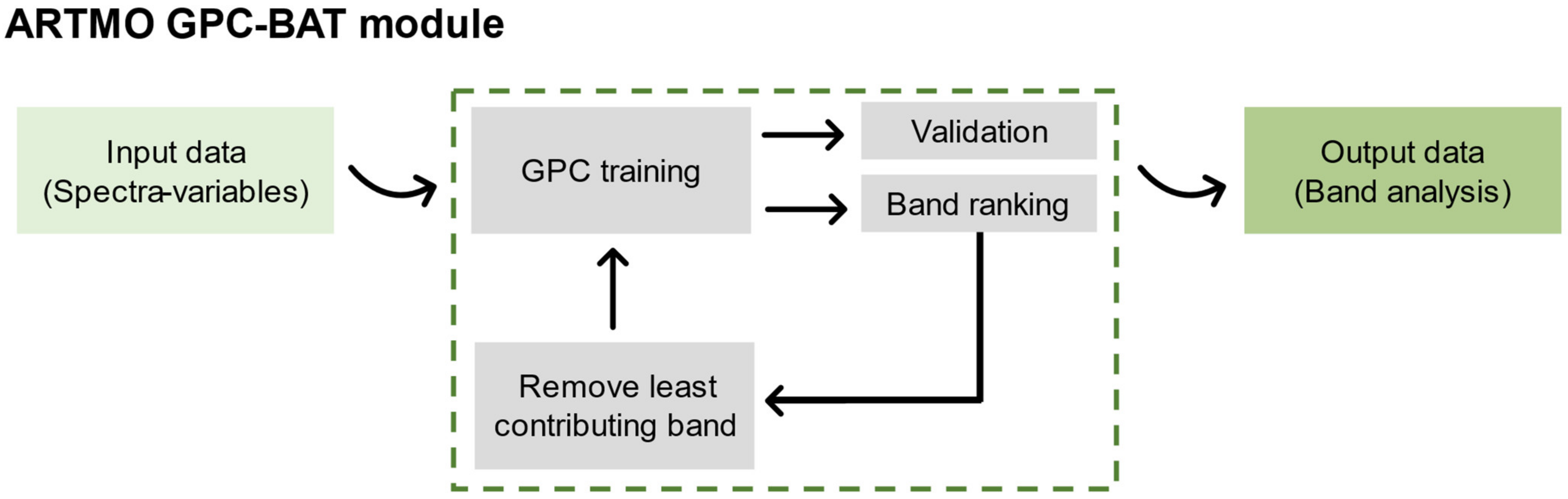
Furthermore, automated band analysis tools have been developed in the domain of machine learning classification algorithms (MLCAs). Following a band selection method earlier introduced in regression [18], this paper introduces an automated spectral band analysis tool (BAT) based on Gaussian process classification (GPC) for the spectral analysis of bacterial plant diseases. Briefly, starting from using all bands, GPC-BAT sequentially removes the least informative band in GPC until one band is left. By tracking the accuracy of statistics, GPC-BAT allows (1) to identify the most informative bands relating spectral data to a classification problem, and (2) to find the least number of bands that preserve optimized accurate classification tasks.

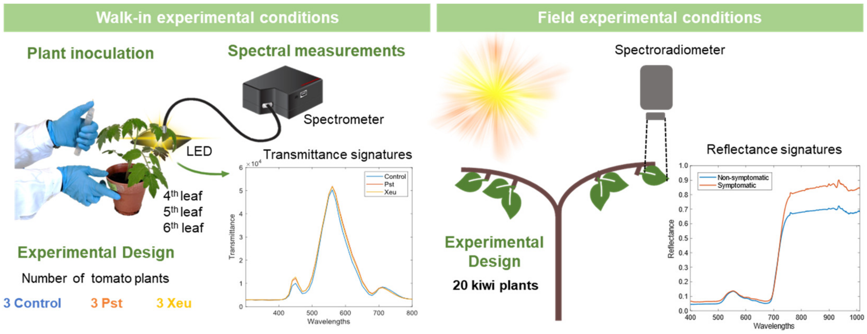
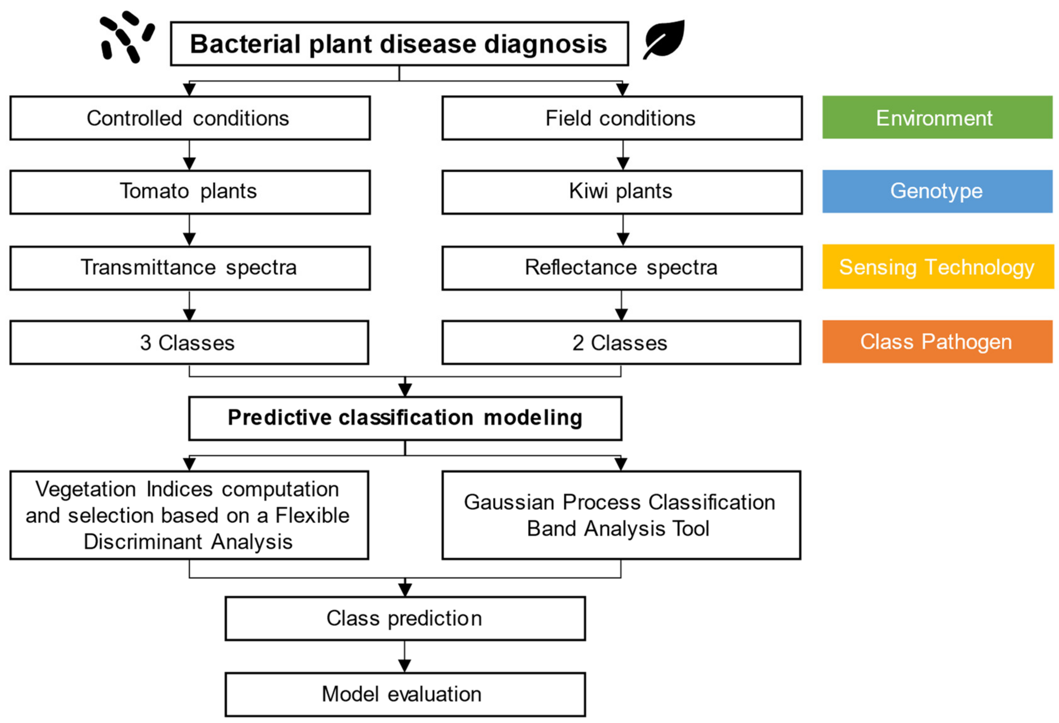
Hence, despite the development and availability of diverse methods for extracting meaningful spectral information in the context of plant bacterial disease diagnosis, it is necessary to address their suitability and performance when leading with different pathosystems. Therefore, the main objective of the present work aimed to explore, test, and validate the application of proximal optical sensed data for the early assessment and diagnosis of bacterial plant diseases. In this regard, the specific goals of this study were: (i) explore the suitability of different VIs for extracting relevant spectral features for performing plant bacterial disease diagnosis, using both reflectance and transmittance hyperspectral data (physiological driven approach); (ii) investigate the potential of a GPC-BAT for performing plant bacterial disease diagnosis using reflectance and transmission hyperspectral data (data-driven approach); (iii) compare and contrast the performance of VIs and GPC-BAT in discerning spectral features crucial for differentiating between healthy and diseased plant tissues; and (iv) uncover the biological significance of the identified spectral features concerning specific plant–pathogen interactions and their implications for early disease diagnosis. To achieve this, two case studies were conducted on tomato (controlled conditions) and kiwi (field conditions) plants, aiming to explore the capabilities of the developed approaches for performing bacterial disease diagnosis in distinct species in different environmental conditions.

2. Materials and Methods

The present analysis focuses on two case studies: one in controlled environmental conditions using hyperspectral transmittance sensing data and the second in field conditions using hyperspectral reflectance sensing data. The first case consisted of collecting spectral data in healthy tomato leaflets’ tissues, along with measurements in inoculated (diseased) tissues with Pseudomonas syringae pv. tomato (responsible for the bacterial speck disease of tomato), and tissues inoculated with Xanthomonas euvesicatoria (responsible for the bacterial spot disease of tomato). The second case assessed spectral data in nonsymptomatic and symptomatic kiwi leaf tissues affected by the bacterial canker of kiwi caused by Pseudomonas syringae pv. actinidiae. In both case studies, multiple spectral samples were gathered within an experimental setup at various time intervals, encompassing all the plants involved in the study.

The hyperspectral data were then used in two modeling approaches involving a physiologically driven parametric approach based on VIs and a nonparametric approach based on a Gaussian Process Classification Banda Analysis Tool.

2.1. Case Studies—Experimental Design for Kiwi and Tomato

2.1.1. Tomato Bacterial Diseases—Indoor Assay

An indoor assay was performed in a walk-in growth chamber (temperature of 25 to 27 °C, humidity of 60% approximately, photoperiod of 12/12 h, and light intensity of 30 W) with nine tomato (Solanum lycopersicum L.) plants of the variety Cherry in 200 mL pots with a commercial potting substrate. Groups of three plants were formed and physically separated from each other to avoid cross-contamination; one group was sprayed with distilled water (Control, healthy class), the second group with a bacterial suspension ($1\times {10}^8\mathrm{c}\mathrm{e}\mathrm{l}\mathrm{l}\mathrm{s}/\mathrm{m}\mathrm{L}$) of Pseudomonas syringae pv. tomato DC 3000 (Pst), and the last group with a suspension ($1\times {10}^8\mathrm{c}\mathrm{e}\mathrm{l}\mathrm{l}\mathrm{s}/\mathrm{m}\mathrm{L}$) of Xanthomonas euvesicatoria (Xeu), following a previously developed protocol [19] (Figure 1). Plant phenotypical observations were performed daily to assess symptom development for 10 days (

Table 1. Spectral data characterization of the measurements randomly performed on tomato leaflets (walk-in chamber—controlled conditions, transmittance) and kiwi leaves (in-field conditions, reflectance), showing the number of assessment dates, plants, and observations (classified according to visual phenotyping observations).

	N° Dates	N° Plants *	N° NS	N° S	Total
Walk-in assay
Tomato	8	9	1365	981	2346
Con		3	809	---	809
Pst		3	93	634	727
Xeu		3	463	347	810
In-field assay (2 sites)
Kiwi	9	20	281	223	504

Control (healthy), Pst—Inoculated with Pseudomonas syringae pv. tomato, Xeu—Inoculated with Xanthomonas euvesicatoria, NS—nonsymptomatic, S—symptomatic. * Several measurements were taken over time on different leaflets on each plant.

).

The success of artificial bacterial inoculation was assessed by the performance of a viability assay and through a colony polymerase chain reaction (PCR), as stated in [19]. PCR analyses were performed at 48, 72, and 96 h after bacterial inoculation, as well as in the last assay date. The growth of Pst and Xeu in their appropriate selective (KB and YDC, respectively) media demonstrated that bacteria were viable at the moment of inoculation. PCR results proved the infection success, where the formation of bacteria-specific bands for each pathogen species, namely a 200-base pair (bp) fragment for Pst and a 713 bp fragment for Xeu, were observed. No PCR amplification was observed from samples collected from Control samples, assuring they were healthy until after the last spectral measurement. The first macroscopic lesions were detected in Pst-inoculated samples 3 days after inoculation (DAI) and in Xeu-inoculated samples at 8 DAI.

Hyperspectral transmittance point-of-measurement (POM) data were captured inside a walk-in chamber using a setup composed of a mini spectrometer (Hamamatsu Photonics K.K. TM Series C11697MB) with a wavelength range of 200–1100 nm, and a spectral resolution of 0.6 nm. This setup includes a transmission optical fiber bundle (FCR-7UVIR200-2-45-BX, Avantes, Eerbeek, The Netherlands), a laptop for data storage and processing, and a white LED spanning from 390 to 800 nm. A specialized evaluation software (SpecEvaluationUSB2.exe, Hamamatsu Photonics K.K., Hamamatsu, Japan) was used for data acquisition. Further details about the setup can be found in previous work [19] (Figure 1). Subsequently, a resampling technique of approximately 10 nm was employed to minimize data redundancy. A dataset comprising 2346 samples (spectral observations) encompassing 51 wavelength features (spectral variables) was selected for subsequent analysis. The spectral measurements were later classified according to the leaflets’ plant treatment group, including the classes: (i) Control (healthy); (ii) inoculated with Pst; and (iii) inoculated with Xeu (Table 1). This dataset can be found in [20].

2.1.2. Kiwi Bacterial Diseased—Field Assay

An assay was performed in field conditions in commercial orchards of kiwi (Actinidia deliciosa) of the cultivar ‘Bo.Erika’, located in Guimarães, Portugal. Macroscopic signs (i.e., symptoms visual to the human eye) of bacterial canker caused by Pseudomonas syringae pv. actinidiae (Psa) were assessed in feminine plants. Plant visual phenotyping was performed, classifying leaves into nonsymptomatic (NS, when no macroscopic visual symptoms were present) or symptomatic (S, when macroscopic symptoms were visible), as described in [21] (Table 1). The detection of Psa in Kiwi samples was carried out by dedicated PCR following the EPPO guideline [22], as detailed by Mariz-Ponte et al. [23]. These samples were collected before the spectral assay and proved the presence of the bacteria in study in the orchards under study.

Hyperspectral reflectance measurements were collected in situ, in vivo leaves, using a portable spectroradiometer (ASD FieldSpec^® HandHeld 2, ASD Instruments, Boulder, CO, USA) with a wavelength range of 325 to 1075 nm, spectral resolution of 1 nm, and field-of-view conical angle of 25° (Figure 1). The detailed procedures followed during the spectral acquisition assay can be found in previous research [21]. In brief, three leaves were chosen per plant, and their spectral signatures were collected at different time points, resulting in 504 samples (spectral observations) and 751 spectral features (spectral variables). Binary classification of leaves’ spectra was made according to the phenotype of the leaves resulting in the binary classes NS and S (Table 1). This dataset can be found in [24].

2.2. Modeling Approaches

Parametric Approach—Vegetation Indices (VIs)

Hyperspectral data, including both transmittance and reflectance spectra, usually have an overlapping nature and multi-scale interference [25]. To address this issue, a selection of 33 spectral VIs, encompassing 42 distinct wavelength combinations, was computed to identify the most relevant wavelengths or bands for discriminating healthy and diseased biological tissues (Table 2) (Figure 2). This selection process aimed to integrate VI formulations commonly used to assess different crop traits as well as crops’ physiological conditions. The variables used in each formula corresponded to default values explicitly mentioned in the formula (Table 2) or values chosen by the authors, namely: 450 nm (representing the blue region of the electromagnetic spectrum), 550 nm (green), 680 nm (red), 700 nm (red edge), and 800 nm (NIR). The feature representing the blue region was elected due to being related to pigment absorption features (~450 nm, e.g., chlorophylls and carotenoids) [26,27] and a blue fluorescence maximum [28]. The 550 nm wavelength was selected because reflectance data correspond to the green peak (or green edge), where reflectance values can be more than twice the surrounding wavelengths [29,30]. This value is also sensitive to chlorophyll content and has been explored to detect plant stress-induced changes and pigment content variations [31,32]. Instead, 680 nm was chosen because it corresponds to the reflectance minimum in the Red region [29,30]. The red-edge value (700 nm) was used because it is highly sensitive to changes in chlorophyll-a absorption and is used to detect subtle changes related to plant physiological status and growth stage transitions [31,33]. The 800 nm spectral feature was chosen because it is related to the influence of changes in leaf structure and density, but it is not sensitive to pigment level changes [34]. Furthermore, all these wavelengths have been extensively used in formulating multiple VIs, as seen in Index Data Base (IDB), a database for remote sensing indices [35,36].

A Flexible Discriminant Analysis (FDA), which applied predictive modeling with a built-in Feature Selection (FS), was then performed to evaluate the most significant VIs used to discriminate between spectral data measured in (i) healthy tomato tissues (Control, Con), diseased tomato tissues inoculated with Pst, and diseased tomato tissues infected with Xeu; and (ii) nonsymptomatic (i.e., without macroscopic lesions, NS) and symptomatic (S) kiwi tissues (Figure 2). The datasets, encompassing both tomato and kiwi cases, were split according to the holdout method [37], which involved partitioning into a training set comprising 70% of the data and a testing set with the remaining 30% of the observations [38].

Model evaluation was employed through a resampling strategy involving repeated 10-fold cross-validation to estimate accuracy. A more detailed explanation can be found in [37,38,39]. Model performance was then evaluated by assessing different classification model metrics, including the confusion Matrix (CM), accuracy score, kappa coefficient, and F1-score [19].

The CM is a 2D-matrix representation of the actual classes of the collected spectral samples in one dimension and the predicted class values in the other. When the predicted class values are equal to the actual value, they are considered correct classifications and localized in the CM’s diagonal. The remaining matrix cells correspond to incorrect classification predictions, where the predicted value is not coincident with the actual value. The class of interest is considered positive, while the other(s) are considered negative. When the predicted class is correctly classified as the class of interest, it is considered a true positive (TP) case. When the predicted class is accurately classified as not belonging to the class of interest, it is called a true negative (TN). When the predicted class is wrongly classified as the class of interest, it is called a false positive (FP), and when incorrectly classified as not fitting the class of interest, it is classified as a false negative (FN).

The accuracy score (also known as Success Rate) corresponds to the number of rightfully classified prediction cases divided by the total number of predictions (Equation (1)):

$$Accuracy=\frac{TP+TN}{TP+TN+FP+FN}$$

(1)

The kappa coefficient (also called Cohen’s kappa) amends the accuracy score by considering the probability of an accurate prediction occurring by chance alone [37] (Equation (2)). Its value can range from zero, indicating an imperfect agreement, to one, the perfect agreement between models’ predictions and true values. Kappa values (in percentage) can be interpreted as follows: when less than 20%, it is considered a poor agreement; 20% to 40%, a fair agreement; 40% to 60%, a moderate agreement; 60% to 80%, a good agreement; and 80% to 100%, a very good agreement [37]. The kappa coefficient can be estimated through the following formula, where Pr(a) represents the proportion of actual agreement and Pr(e) refers to the expected agreement between the classifier and the true values, under the hypothesis that they were chosen randomly (Equation (2)):

$$Kappa coefficient=\frac{\mathit{Pr}\left(a\right)-\mathit{Pr}\left(e\right)}{1-\mathit{Pr}\left(e\right)}$$

(2)

The F1-score (also called F-measured) combines the proportion of positive cases that are truly positive (Precision) with the number of TP over the total number of positives (Recall, which measures how complete the results are) into a single number using the harmonic mean (Equation (3)):

$$F-score=\frac{2\times precision\times recall}{recall+precision}=\frac{2\times TP}{2\times TP+FP+FN}$$

(3)

Sensitivity was evaluated, indicating the models’ ability to predict the TP of each available class (Equation (4)):

$$Sensitivity=\frac{TP}{TP+FN}$$

(4)

The Specificity metric was also calculated, since it indicates the models’ suitability for predicting TN of each available class (Equation (5)):

$$Specificity=\frac{TN}{TN+FP}$$

(5)

All these computation analyses were made in the software R [40] (v. 4.2.1) using the packages ‘caret’ [41] and ‘earth’ [42]. The previous formulae can also be found in [41].

Table 2. List of the Spectral Vegetation Indices (VIs) computed in this work, mentioning their formula and reference (when available).

Vegetation Indices	Formula	Ref.
Ashburn Vegetation Index (AVI)	$2.0\times NIR-RED$	[43,44]
Anthocyanin reflectance index (ARI)	$\frac{1}{GREEN}-\frac{1}{RED}$	[45]
Blue Green Pigment Index (BGI)	$\frac{BLUE}{GREEN}$	-
Browning Reflectance Index (BRI)	$\frac{\frac{1}{GREEN}-\frac{1}{RED}}{NIR}$	[46]
Blue/Red Pigment Index (BRI2)	$\frac{450 \mathrm{n}\mathrm{m}}{690 \mathrm{n}\mathrm{m}}$	[47]
Canopy Chlorophyll Content Index (CCI)	$\frac{\frac{NIR-RED EDGE}{NIR+RED EDGE}}{\frac{NIR-RED}{NIR+RED}}$	[48,49,50,51,52,53]
Chlorophyll Green (Chlgreen)	${\left(\frac{NIR}{GREEN}\right)}^{(-1)}$	[54]
Coloration Index (CI)	$\frac{RED-BLUE}{RED}$	[55]
Chlorophyll Index Green (CIgreen)	$\frac{NIR}{GREEN}-1$	[56,57,58]
Chlorophyll Index Red Edge (CIrededge)	$\frac{NIR}{RED EDGE}-1$	[56,57,58]
Chlorophyll vegetation index (CVI)	$NIR \times \frac{RED}{{GREEN}^2}$	[59]
Double Difference Index (DD)	$(749 \mathrm{n}\mathrm{m}-720 \mathrm{n}\mathrm{m})-(701 \mathrm{n}\mathrm{m}-672 \mathrm{n}\mathrm{m})$	[60,61]
Enhanced Vegetation Index (EVI)	$2.5\times \frac{NIR-RED}{\left(NIR+6RED-7.5BLUE\right)+1}$	[58,62]
Green atmospherically resistant vegetation index (GARI)	$\frac{NIR-(GREEN-(BLUE-RED\left)\right)}{NIR-(GREEN+(BLUE-RED\left)\right)}$	[57,63]
Green-Blue NDVI (GBNDVI)	$\frac{NIR-\left(GREEN+BLUE\right)}{NIR+\left(GREEN+BLUE\right)}$	[64]
Global Environment Monitoring Index (GEMI)	$\left(n\times \left(1-0.25n\right)-\frac{RED-0.125}{1-RED}\right)$ $n=\frac{2\times \left({NIR}^2-{RED}^2\right)+1.5\times NIR+0.5\times RED}{NIR+RED+0.5}$	[65]
Simple Ratio Greenness Index (GI)	$\frac{GREEN}{RED}$	[61,66]
Green Normalized Difference Vegetation Index (GNDVI)	$\frac{NIR-GREEN}{NIR+GREEN}$	[56,58]
Tasseled Cap—vegetation (GVI)	$$\begin{gathered} -0.2848\times Blue-0.2435\times Green-0.5436\times Red+ \\ 0.7243\times NIR+0.0840\times SWIR-0.1800\times SWIR \end{gathered}$$	[67,68]
Infrared percentage vegetation index (IPVI)	$\frac{\frac{NIR}{NIR+RED}}{2}\times (NDVI+1)$	[69,70]
Log Ratio (LogR)	$log\left(\frac{NIR}{RED}\right)$	-
Misra Green Vegetation Index (MGVI)	$\begin{array}{cc}-0.386\times GREEN& - 0.530\times RED+0.535\times REDEDGE\\ & +0.532\times NIR\hfill \end{array}$	[44,71]
Modified NDVI (mNDVI)	$\frac{NIR-RED}{NIR+RED-2\times BLUE}$	[61,72]
Modified Simple Ratio (mSR)	$\frac{NIR-BLUE}{RED-BLUE}$	[61,70]
Modified Simple Ratio 2 (mSR2)	$\left(\frac{NIR}{RED}\right)-\frac{1}{\sqrt{\left(\frac{NIR}{RED}\right)+1}}$	[73]
Normalized Difference NIR/Red Normalized Difference Vegetation Index (NDVI)	$\frac{NIR-RED}{NIR+RED}$	[74,75]
Normalized Green (NG)	$\frac{GREEN}{NIR+RED+GREEN}$	[68]
Normalized Near Infrared (NNIR)	$\frac{NIR}{NIR+RED+GREEN}$	[68]
Hyperspectral perpendicular VI (PVIhyp)	$\frac{NIR-a\times 807-b}{{(1+a^2)}^{0.5}}$ $a=1.17, b=3.37$	[68]
Plant Senescence Reflectance Index (PSRI)	$\frac{RED-BLUE}{NIR}$	[76,77]
Reflectance at the inflection point (Rre)	$\frac{RED+NIR}{2}$	[78]
Red-Edge Stress Vegetation Index (RVSI)	$\frac{718+748}{2}-733$	-
Structure Intensive Pigment Index (SIPI)	$\frac{NIR-BLUE}{NIR-RED}$	[60,66]
Simple Ratio (SR) NIR/RED	$\frac{NIR}{RED}$	-

Table 2. List of the Spectral Vegetation Indices (VIs) computed in this work, mentioning their formula and reference (when available).

Vegetation Indices	Formula	Ref.
Ashburn Vegetation Index (AVI)	$2.0\times NIR-RED$	[43,44]
Anthocyanin reflectance index (ARI)	$\frac{1}{GREEN}-\frac{1}{RED}$	[45]
Blue Green Pigment Index (BGI)	$\frac{BLUE}{GREEN}$	-
Browning Reflectance Index (BRI)	$\frac{\frac{1}{GREEN}-\frac{1}{RED}}{NIR}$	[46]
Blue/Red Pigment Index (BRI2)	$\frac{450 \mathrm{n}\mathrm{m}}{690 \mathrm{n}\mathrm{m}}$	[47]
Canopy Chlorophyll Content Index (CCI)	$\frac{\frac{NIR-RED EDGE}{NIR+RED EDGE}}{\frac{NIR-RED}{NIR+RED}}$	[48,49,50,51,52,53]
Chlorophyll Green (Chlgreen)	${\left(\frac{NIR}{GREEN}\right)}^{(-1)}$	[54]
Coloration Index (CI)	$\frac{RED-BLUE}{RED}$	[55]
Chlorophyll Index Green (CIgreen)	$\frac{NIR}{GREEN}-1$	[56,57,58]
Chlorophyll Index Red Edge (CIrededge)	$\frac{NIR}{RED EDGE}-1$	[56,57,58]
Chlorophyll vegetation index (CVI)	$NIR \times \frac{RED}{{GREEN}^2}$	[59]
Double Difference Index (DD)	$(749 \mathrm{n}\mathrm{m}-720 \mathrm{n}\mathrm{m})-(701 \mathrm{n}\mathrm{m}-672 \mathrm{n}\mathrm{m})$	[60,61]
Enhanced Vegetation Index (EVI)	$2.5\times \frac{NIR-RED}{\left(NIR+6RED-7.5BLUE\right)+1}$	[58,62]
Green atmospherically resistant vegetation index (GARI)	$\frac{NIR-(GREEN-(BLUE-RED\left)\right)}{NIR-(GREEN+(BLUE-RED\left)\right)}$	[57,63]
Green-Blue NDVI (GBNDVI)	$\frac{NIR-\left(GREEN+BLUE\right)}{NIR+\left(GREEN+BLUE\right)}$	[64]
Global Environment Monitoring Index (GEMI)	$\left(n\times \left(1-0.25n\right)-\frac{RED-0.125}{1-RED}\right)$ $n=\frac{2\times \left({NIR}^2-{RED}^2\right)+1.5\times NIR+0.5\times RED}{NIR+RED+0.5}$	[65]
Simple Ratio Greenness Index (GI)	$\frac{GREEN}{RED}$	[61,66]
Green Normalized Difference Vegetation Index (GNDVI)	$\frac{NIR-GREEN}{NIR+GREEN}$	[56,58]
Tasseled Cap—vegetation (GVI)	$$\begin{gathered} -0.2848\times Blue-0.2435\times Green-0.5436\times Red+ \\ 0.7243\times NIR+0.0840\times SWIR-0.1800\times SWIR \end{gathered}$$	[67,68]
Infrared percentage vegetation index (IPVI)	$\frac{\frac{NIR}{NIR+RED}}{2}\times (NDVI+1)$	[69,70]
Log Ratio (LogR)	$log\left(\frac{NIR}{RED}\right)$	-
Misra Green Vegetation Index (MGVI)	$\begin{array}{cc}-0.386\times GREEN& - 0.530\times RED+0.535\times REDEDGE\\ & +0.532\times NIR\hfill \end{array}$	[44,71]
Modified NDVI (mNDVI)	$\frac{NIR-RED}{NIR+RED-2\times BLUE}$	[61,72]
Modified Simple Ratio (mSR)	$\frac{NIR-BLUE}{RED-BLUE}$	[61,70]
Modified Simple Ratio 2 (mSR2)	$\left(\frac{NIR}{RED}\right)-\frac{1}{\sqrt{\left(\frac{NIR}{RED}\right)+1}}$	[73]
Normalized Difference NIR/Red Normalized Difference Vegetation Index (NDVI)	$\frac{NIR-RED}{NIR+RED}$	[74,75]
Normalized Green (NG)	$\frac{GREEN}{NIR+RED+GREEN}$	[68]
Normalized Near Infrared (NNIR)	$\frac{NIR}{NIR+RED+GREEN}$	[68]
Hyperspectral perpendicular VI (PVIhyp)	$\frac{NIR-a\times 807-b}{{(1+a^2)}^{0.5}}$ $a=1.17, b=3.37$	[68]
Plant Senescence Reflectance Index (PSRI)	$\frac{RED-BLUE}{NIR}$	[76,77]
Reflectance at the inflection point (Rre)	$\frac{RED+NIR}{2}$	[78]
Red-Edge Stress Vegetation Index (RVSI)	$\frac{718+748}{2}-733$	-
Structure Intensive Pigment Index (SIPI)	$\frac{NIR-BLUE}{NIR-RED}$	[60,66]
Simple Ratio (SR) NIR/RED	$\frac{NIR}{RED}$	-

2.3. ARTMO Software

The Automated Radiative Transfer Models Operator (ARTMO) is a modular MATLAB GUI toolbox initially developed for automating the simulation of radiative transfer models (RTMs) [79]. This comprehensive toolbox integrates various leaf and canopy RTMs alongside essential tools for semi-automated retrieval of biophysical and biochemical variables. ARTMO (v. 3.31) is connected to a relational SQL database management system (MySQL, version 5.5 or 5.6; local installation required) for storing all generated data (i.e., simulations and statistical results) and trained models along with metadata, enabling the re-execution of earlier models or simulations. An initial version of the machine learning classification algorithm (MLCA) toolbox was introduced in version 3.29, and this functionality has been expanded in subsequent releases.

The current official version (v.1.02) of the MLCA toolbox incorporates 20 supervised MLCAs belonging to the principal families of supervised classifiers, predominantly affiliated with machine learning methodologies. Note that this initial version is limited to pixel-based classifiers, implying that object-based subpixel-based or scene-based deep learning classifiers have not been incorporated. Nevertheless, pixel-based classifiers enable the learning and characterization of intricate spectra.

Supervised classifiers are traditionally classified into parametric and nonparametric methods. Parametric methods are grounded in probabilistic theories, modeling the decision boundaries between classes from a fixed number of parameters, independent of the number of samples, employing global criteria for classification [80]. By contrast, nonparametric methods guide the class grouping based on the digital number (single band/image) or spectral data (multi- and hyperspectral reflectance or transmittance). The spectral value distribution is independent and focused on the local data structure, requiring a substantial set of samples for the classification process [81].

Arguably, one of the most promising nonparametric classifiers is the Gaussian process (GP) classification. GPs are stochastic processes where each random variable follows a multivariate normal distribution [82]. The goal of GP classification is to learn a mapping from the input data (e.g., spectral reflectance or transmittance values) to their corresponding classification label (e.g., plant health group type), which can then be used on new, unseen spectral measurements (Figure 2). When the GP is developed with kernel methods [83], it allows mapping the original data into a possibly infinite-dimensional space [84]. In this space, the input–output relationship can be better estimated as the GP can consider more complex and flexible functions than the linear models. This enables the GP to capture intricate relationships between the spectral data and the health crop phenotype, leading to more accurate classification results. Due to its probabilistic framework, the GP provides uncertainty estimation per sample. This means that for each spectral measurement, the GP can provide a measure of how confident it is in its classification prediction. This uncertainty information can inform decision making, allowing users to be more or less confident with the inferred classification label (e.g., see [15]).

Machine Learning Approaches—Gaussian Process Classification (GPC-BAT)

The GP has another advantage of being capable of using more sophisticated kernel functions than the standard linear kernel or the radial basis function (RBF) kernel equation (Equation (6)), which can be optimally tuned through likelihood maximization:

$$k_{RBF}\left(x_i,x_j\right)=exp\left(-\frac{{‖x_i-x_j‖}^2}{2{\sigma }^2}\right)$$

(6)

where $x_i$ and $x_j$ represent two spectra, σ is the variance, and $‖x_i-x_j‖$ is the Euclidean distance between the two spectra $x_i$ and $x_j$ [18,82].

In the classification case, the output values of $k_{RBF}$ are discrete (±1); this causes the likelihood function to be non-Gaussian, and then some approximations should be performed [85]. We chose the Laplace approximation which performs well and is robust. One notable kernel function is the automatic relevance determination (ARD) kernel equation (Equation (7)):

$$K_{ARD}\left(x_i,x_j\right)=\mathrm{e}\mathrm{x}\mathrm{p}\left(-\frac{1}{2}{\left(x_i,x_j\right)}^{\mathrm{\top }}{\sum }^{-1}\left(x_i,x_j\right)\right)$$

(7)

where Σ is a diagonal matrix, whose diagonal tries are constituted by $\left\{{\sigma }_1^2,\dots ,{\sigma }_d^2\right\}$ parameters to weight each input dimension [18,82]. This kernel covariance function requires one parameter per input feature; it can be optimized under that framework, and it allows providing a band ranking based on their optimal values.

Following the rationale as presented in Verrelst et al. (2016) [18] for GP regression, a GPC-based band ranking feature has been implemented into a so-called band analysis tool (i.e., GPC-BAT). In short, we employ a simplified and general iterative backward greedy algorithm to identify the most informative bands. This algorithm assesses the impact of each band on the prediction error in the context of the remaining bands. At each iteration, the algorithm removes the band with the highest uncertainty σb, thereby re-training the GPC model with the remaining bands. This is referred to as sequential backward band removal (SBBR). The SBBR algorithm is analogous to recursive feature elimination (RFE), a technique earlier presented with support vector machines or random forests. In RFE, the feature with the lowest ranking score is eliminated, iteratively removing insignificant features until only the most relevant ones remain (e.g., [86,87,88,89]). This SBBR approach allows us to pinpoint the bands that most strongly influence the prediction of our target classes. These bands provide valuable insights into the spectral characteristics that best capture the sensitivity of the classes of interest, e.g., healthy and diseased groups.

A principal application of GPC-BAT is that the algorithm identifies how many bands are minimally needed in order to retain robust results and informs us about the most sensitive wavelengths. Accordingly, the output GUI delivers the following band analysis outputs: (1) overall accuracy (OA) statistics as a function of #bands plotted over the sequentially removed bands until only two bands are left and (2) associated wavelengths selected by the tool (Figure 3).

3. Experimental Results

3.1. Spectral Vegetation Indices—Parametric Approach

This section presents the predictive classification results of the approach combining the calculation of different VIs (

Table 3. Cross-validation statistics of the Flexible Discriminant Analysis (FDA) using the validation set of the Vegetation Indices (VIs) computed in the hyperspectral data collected on tomato leaflet tissues (transmittance) and kiwi leaf tissues (reflectance). Model metrics by class are also provided.

	Overall Classes		Metrics per Class
Class	Accuracy (%)	Kappa (%)	Precision (%)	Sensitivity (%)	Specificity (%)	F1 (%)
Tomato (703 observations)
Con	63.33	44.77	63.67	76.03	77.22	69.30
Pst			75.66	65.60	90.52	70.27
Xeu			52.44	48.56	76.74	50.43
Kiwi (504 observations)
NS/S	71.33	41.73	67.69	66.67	75.00	67.18

Con—Control (healthy), Pst—Inoculated with Pseudomonas syringae pv. tomato, Xeu—Inoculated with Xanthomonas euvesicatoria, NS—nonsymptomatic, S—symptomatic.

) followed by the computation of the FDA model, which allowed (i) the classification of tomato leaflet spectral samples collected on healthy (Control, Con) and both inoculated diseased tissues with Pst and Xeu bacteria; and (ii) the classification of kiwi leaf spectral samples measured on nonsymptomatic (NS) and symptomatic (S) diseased tissues.

3.1.1. Tomato Disease in Walk-In Chamber

Table 2 presents the results of an overall accuracy of 63.30% (proportion of correctly classified instances) and a kappa coefficient of 44.70 (which indicates agreement between the predicted and actual classes beyond random occurrence) for the validation dataset (Table 3, detailed information about the training results is present in Supplementary Materials Table S1). The model metric analysis per class revealed that samples inoculated with Pst bacteria presented good precision (75.66%), sensitivity (65.60%), specificity (90.52%), and F1-score (70.27%) (Table 3). These metrics indicate the model’s suitability for accurately performing correct predictions for both classes (healthy vs. inoculated), correctly identifying instances of these classes, distinguishing samples that do not belong to these classes, and a good balance in capturing true positives and avoiding false positives (Table 3). The control class presented a higher sensitivity, highlighting the model’s efficiency in correctly identifying healthy samples. In contrast, the Xeu class had a reduced precision (52.44%), sensitivity (48.56%), and F1-score (50.43%), which translates into a higher likelihood of false positives in Xeu prediction, a more probable miss of a considerable proportion of positive instances of this class, and an imbalance in assessing true positives and avoiding false positives (Table 3). Therefore, although the FDA model exhibits good capabilities in differentiating samples measured in healthy (Control) and Pst-diseased tissues, there is potential for improving the identification of spectra captured on Xeu-inoculated tissues (Table 3).

A fraction of these false positives may be accounted for by the sensitivity gap between digital and visual phenotyping methods. These results are based on visual phenotyping, which only allows samples with visible symptoms to be identified. However, Xeu-inoculated plants may present early changes in their optical properties long before the appearance of symptoms, which could justify some of the false positive cases recorded.

CM results indicate that predictions of samples collected on tissues inoculated with Xeu were more challenging to the model when compared to the healthy and inoculated with Pst ones, presenting a higher number of wrong classifications than in the remaining classes studied (

Table 4. Confusion Matrix results of the Flexible Discriminant Analysis (FDA) using the Vegetation Indices (VIs) computed in the hyperspectral data collected on tomato leaflet tissues (transmittance) and kiwi leaf tissues (reflectance). The predicted samples of each class (column) that were correctly classified for each true class (row) for the spectral data collected on tomato leaflets tissues (left) and kiwi leaf tissues (right) are shown. The classes used in the tomato case study were control samples (healthy, Con), samples inoculated with Pseudomonas syringae pv. tomato (Pst), and samples inoculated with Xanthomonas euvesicatoria (Xeu). In turn, the binary classes nonsymptomatic (NS) and symptomatic (S) were applied to the kiwi case study.

		Predicted Class—Tomato							Predicted Class—Kiwi
		Training			Validation				Training		Validation
		Con	Pst	Xeu	Con	Pst	Xeu		NS	S	NS	S
True Class	Con	416	10	141	184	4	54	NS	157	40	63	21
	Pst	52	345	112	22	143	53	S	50	107	22	44
	Xeu	193	90	284	83	42	118

, for both training and validation sets). In fact, the model only correctly identified 49.63% of the total Xeu samples. The majority of the remaining Xeu samples were wrongly inputted to the Control class. This can be related to the fact that macroscopic symptoms only appeared 8 DAI, resulting in a high number of nonsymptomatic samples (presenting a phenotype similar to the healthy ones), whose spectral signature is more similar to healthy samples than Pst-diseased ones. In contrast, approximately 74.17% of the total healthy (Control) samples were accurately classified and 67.13% of the total number of samples inoculated with Pst (Table 4).

3.1.2. Kiwi Bacterial Canker Disease in the Field

In turn, when the IVs-based modeling approach was applied in the binary classification of nonsymptomatic (NS in Table 3) and symptomatic (S in Table 3) samples of the validation set taken on kiwi leaves in field conditions, the overall accuracy achieved was 71.33%. The kappa value of 41.73% demonstrates the model’s effectiveness in classifying the two classes (results for the training set can be seen in Supplementary Materials Table S1). The model metrics for the spectra collected in nonsymptomatic and symptomatic tissue’s spectra revealed that the model acceptably identifies a significant proportion of true positive samples of these classes, classifies samples belonging to both classes, and has a good ability to correctly identify instances that do not belong to the class in analysis, along with a good balance between finding positive cases and avoiding false positives (Table 3).

The CM values show that the model has less difficulty predicting nonsymptomatic samples correctly classifying 78.28% of the total samples compared to the symptomatic samples (67.71%) (Table 4).

3.2. GPC-BAT Performance with Original Training Data and Further Validation

This section presents the predictive classification results of the approach using the ARTMO GPC-BAT tools, which also allowed (i) the classification of tomato leaflet spectral samples collected on healthy (Control, Con), Pst-inoculated, and Xeu-inoculated tissues and (ii) the classification of kiwi leaf spectral samples measured on nonsymptomatic (NS) and symptomatic (S) tissues.

3.2.1. Tomato Diseases in Walk-In Chamber

For the selected 23 wavelengths (from the 51 available) for the tomato case study and 577 wavelengths (from the 611) for the kiwi case study, the models presented the best classification metrics (

Table 5. Cross-validation statistics of the Gaussian Process Classification (GPC) models developed using hyperspectral data collected on tomato leaflet tissues (transmittance) and kiwi leaf tissues (reflectance).

	Overall Classes		Metrics per Class
Class	Accuracy (%)	Kappa (%)	Precision (%)	Sensitivity (%)	Specificity (%)	F1 (%)
Tomato
Con	70.46	55.60	80.72	68.09	88.75	73.87
Pst			75.24	79.51	89.14	77.31
Xeu			55.93	64.81	78.32	60.04
Kiwi
NS	75.40	49.95	79.36	77.16	73.02	78.25
S			70.40	73.02	77.16	71.69

Con—Control (healthy), Pst—Inoculated with Pseudomonas syringae pv. tomato, Xeu—Inoculated with Xanthomonas euvesicatoria, NS—nonsymptomatic, S—symptomatic.

). The prediction for discriminating the different classes defined for the tomato dataset achieved a maximum overall accuracy of 70.46% and kappa of 55.60%. Furthermore, metric evaluation per class provides insights into the model’s performance in distinguishing between healthy (Con in Table 5) and diseased instances (Pst and Xeu in Table 5). In terms of Precision (80.72 vs. 75.24%), Specificity (88.75 vs. 89.14%), and F1-values (73.87 vs. 77.31%), the Control and Pst-inoculated classes presented good metric levels. These results highlight the model’s accuracy in identifying positive predictions for both classes, distinguishing samples that do not belong to these respective classes and achieving a good balance in capturing true positives and avoiding false positives (Table 5). The Xeu-inoculated class, compared with Pst, showed lower values of Precision (55.93 vs. 75.24%) and F1-score (60.04 vs. 71.31%), indicating a higher likelihood of false positives in their prediction and an imbalance in assessing true positives and avoiding false positives. This class had a good Specificity value, similar to the other two, suggesting the model’s performance in distinguishing spectral measurements that do not belong to it (Table 5). Regarding Sensitivity, the Pst class presented the higher level, indicating the model’s effectiveness in correctly identifying instances of this class. However, the values for the two remaining classes were lower, implying that the model may miss a notable proportion of positive instances in the Control and Xeu classes (Table 5).

The CM also demonstrates that 81% of the healthy and 75% of Pst-inoculated samples were correctly classified. Similar to the previous approach (based on VIs), the GPC-BAT also faced more difficulty in accurately classifying the inoculated Xeu samples, with only predicting 56% of the cases correctly (

Table 6. Confusion Matrix of the GPC model results show the predicted samples of each class (column) correctly classified for each true class (row) for the spectral data collected on tomato leaflets’ tissues and kiwi leaf tissues. The classes used in the tomato case study were Control samples (healthy, Con), samples inoculated with Pseudomonas syringae pv. tomato (Pst), and samples inoculated with Xanthomonas euvesicatoria (Xeu). The binary class nonsymptomatic (NS) and symptomatic (S) were applied to the kiwi case study.

		Predicted Class—Tomato							Predicted Class—Kiwi
		Training			Validation				Training		Validation
		Con	Pst	Xeu	Con	Pst	Xeu		NS	S	NS	S
True Class	Con	595	48	221	653	52	254	NS	232	32	223	66
	Pst	31	512	89	38	547	103	S	21	169	58	157
	Xeu	102	95	419	118	128	453

). Hence, while the model demonstrates strong capabilities in distinguishing samples collected in Control (healthy) tissues and those measured on Pst-diseased tissues, it needs to be enhanced to accurately identify spectra collected on Xeu-diseased tissues (Table 5).

3.2.2. Kiwi Bacterial Canker Disease in the Field

The binary classification performed for the kiwi leaves hyperspectral reflectance measurements achieved a maximum overall accuracy of 75.40% and a kappa of 49.95%. The model proved effective in both class predictions, allowing the distinction between nonsymptomatic (NS in Table 5) and symptomatic (S in Table 5) assessments collected in kiwi leaves in field conditions. The model metrics for the spectra collected in nonsymptomatic and symptomatic tissue’s spectra revealed that the model effectively identifies a significant proportion of true positive samples of these classes, a good ability to classify instances that do not belong to them correctly, and a well-balanced between identifying positive instances and avoiding false positives (Table 5).

The CM demonstrates that 79% of the nonsymptomatic samples were accurately classified, along with 70% of the symptomatic samples (Table 6).

The GPC model did not perform best for both case studies when all the spectral bands were applied. In the tomato case study, the overall accuracy and kappa values when all spectral features were used were lower, reaching 69.06% and 53.48%, respectively. Likewise, the kiwi case study’s values were 61.90% and 22.50% for accuracy and kappa, respectively. Furthermore, for the kiwi case study, the outcomes were more unstable when compared to the model developed with the wavelengths chosen by BAT, presenting a higher standard deviation (SD) and processing time (

Table 7. Cross-validation statistics of the GPC models developed using hyperspectral data collected on tomato leaflet tissues (transmittance) and kiwi leaf tissues (reflectance) were used.

SD	Time (s)	FS	Wavelengths (nm)
Tomato
2.75	819.20	51	All wavelengths (300.09 to 800.34 nm)
3.32	491.08	23	430.00, 440.21, 450.04, 460.31, 490.04, 500.00, 510.41, 520.00, 550.20, 560.31, 570.03, 620.21, 640.35, 650.24, 660.15, 670.08, 680.02, 690.42, 700.41, 710.41, 740.09, 750.17, 760.26
Kiwi
4.49	171.86	611	All wavelengths (400 to 1010 nm)
3.23	14.80	34	544, 597, 754, 771, 790, 791, 795, 825, 835, 839, 845, 850, 851, 860, 864, 866, 869, 881, 883, 888, 893, 902, 905, 906, 928, 932, 939, 945, 947, 973, 980, 993, 999, 1006

FS—Feature Selection, SD—Standard Deviation.

). In the tomato case study, the SD value was lower when all the features were used, but the processing time was almost 40% superior (Table 7).

In terms of selected sensitive wavelengths, when the spectral data collected on kiwi were used, GPC profusely selected wavelengths greater than 800 nm (26 of 34 wavelengths), these wavelengths (>800 nm) did not prove to be important in the construction of the selected VIs. Only PVIhyp (800, 1000 nm) selected wavelengths at 800 nm, but this VI has a very modest representation (24.46%) in the distinction between the nonsymptomatic and symptomatic classes.

3.3. Comparing the Performance of VIs and GPC-BAT

3.3.1. Models’ Metric-Based Comparison

The tested approach combining the VIs with the FDA model allowed the identification of the most relevant VIs analyzed for class identification for both the tomato and kiwi case studies (

Table 8. Vegetation Index (VI) importance for classification according to Flexible Discriminant Analysis (FDA). The importance value corresponds to the t-statistic value scaled to the maximum.

Case Study—Tomato			Case Study—Kiwi
VI	Wavelengths (nm)	Importance (a.u.)	VI	Wavelengths (nm)	Importance (a.u.)
mSR2	700.41, 750.17	100.00	Chlgreen	553, 800	100.00
BRI2	450.04, 690.42	70.30	mSR2	705, 750	67.15
GEMI	680.02, 800.34	42.92	CI	450, 700	52.94
PSRI	550.20, 680.02, 750.17	31.69	GI	554, 677	44.45
CCCI	550.20, 700.41, 800.34	27.59	BRI2	450, 690	40.55
EVI	450.04, 680.02, 800.34	22.41	AVI	400, 994	33.71
SIPI	450.04, 680.02, 800.34	16.50	PVIhyp	8,001,000	24.46
Chlgreen	550.20, 730.04	10.71	Chlgreen	530, 730	19.65
SIPI	500.00, 690.42, 800.34	6.66	Rre	670, 780	16.46
GARI	450.04, 550.20, 680.02, 800.34	0.00

AVI—Ashburn Vegetation Index, BRI2—Blue/Red Pigment Index, CCCI—Canopy Chlorophyll Content Index, Chlgreen—Chlorophyll Green, CI—Coloration Index, EVI—Enhanced Vegetation Index, GEMI—Global Environment Monitoring Index, GI—Simple Ratio Greenness Index, mSR2—Modified Simple Ratio, PSRI—Plant Senescence Reflectance Index, PVIhyp—Hyperspectral perpendicular Vegetation Index, Rre—Reflectance at the inflection point, and SIPI—Structure Intensive Pigment Index.

). When the tomato spectral data were used, the selected wavelength combinations present in the computed VIs considered features in the blue region (450.04 nm), green region (500.00, and 550.20 nm), red-edge region (680.02, 690.42, 700.41, 730.04, and 750.17), and NIR region (800.34 nm). Similar wavelengths were selected when the data collected on kiwi leaves were used and were mainly located in the blue region (400, and 450 nm), green region (530, 553, and 554 nm), red-edge region (670, 677, 700, 705, 730, and 750 nm), and NIR region (780, 800, 994, and 1000 nm) (Table 8). For both species, equal wavelengths were identified by the approach, such as 450 (blue), 550 (green), 700, 730, 750 (red-edge), and 800 nm (NIR).

For the tomato case study, the FDA selected five VIs whose formula integrated three wavelengths: PSRI, CCCI, EVI, SIPI, and GARI (Table 8). In contrast, in the kiwi case study, all the chosen VIs presented only two wavelengths (Table 8).

The spectral wavelengths identified by GPC-BAT as the most sensitive for performing bacterial plant disease diagnosis in tomato (in controlled environmental conditions) were mainly located in the blue region (430.00, 440.21, 450.04, and 460.31 nm), green region (510.41, 520.00, 550.20, and 560.31 nm), red region (640.35, 650.24, and 660.15 nm), and red-edge region (670.08, 680.02, 690.42, 700.41, 710.41, 740.09, 750.17, and 760.26 nm) (Table 5, Figure 4). In turn, the model identified the most sensitive features for discriminating in field diseased kiwi leaves infected with bacterial canker (caused by Psa) as mainly occurring in the green region (544, and 597 nm), red-edge region (754 nm), and NIR region (771, 790, 791, 795, 825, 835, 839, 845, 850, 851, 860, 864, 866, 869, 881, 883, 888, 893, 902, 905, 906, 928, 932, 939, 945, 947, 973, 980, 993, 999, and 1006 nm) (Table 5, Figure 5). Similar features were only selected for the two species in the green (550.20 vs. 544 nm) and red-edge (750.17 vs. 754 nm) spectral regions. In contrast, the blue and red spectral regions were only considered in the tomato case study, and the NIR region was considered only in the kiwi case study (since only the spectral sensor used in this assay had wavelengths assessed in these regions) (Table 5).

Both approaches, the one using VIs and FDA and the one using the GPC-BAT, for the tomato case study, selected coincident wavelengths in the blue region (450.04 nm), green region (550.20 nm), and red-edge region (680.02, 690.42, 700.41, and 750.17 nm). The same consistency was not observed for the kiwi case study since different features were chosen. Nevertheless, these were similar in the red-edge region (750 vs. 754 nm) and NIR region (795 vs. 800 nm, 994 vs. 993 nm, and 999 vs. 1000 nm) (Table 5).

In GPC-BAT, the predictive power of each wavelength for the target variable is evaluated by the index sigma (σ). Accordingly, the lower the sigma value, the more important the feature is. Thus, the contribution of each spectral feature can be ranked through the quantification of this property. In the tomato case study, for the selected spectral features, it is possible to observe in Figure 4 that for the identification of the Control (Con) class, 440.21, 450.00, 460.31, 490.04, 510.41, 520.00, 640.35, 680.02, and 750.17 nm were the more relevant wavelengths, since they presented a lower sigma value (i.e., more weight in model), leading to a higher distance from the plots’ center (blue dots). The most significant features for predicting samples made on tomato leaflet tissues inoculated with Pst were 440.21 and 450.04 nm (red dots). In classifying samples collected on leaflet tissues inoculated with Xeu, the 440.21, 450.04, 660.15, and 680.02 nm wavelengths were the most significant for prediction (orange dots). In turn, in the kiwi dataset, from the selected wavelengths, the identification of samples belonging to both classes was more influenced by the 597, 771, 791, 835, 869, 883, 902, and 999 nm features (Figure 5). The wavelengths selected as relevant for the classification of nonsymptomatic samples are the same as those chosen to predict the opposing symptomatic class (Figure 5). This tendency was expected, since this is a binary classification task, where the differences between the two categories in the study are expected to occur in coincident spectral features.

3.3.2. Biological Interpretation of Sensitive Wavelengths

These wavelengths chosen in both case studies present an interesting biological significance, since they coincide with the spectral absorption regions of several photosynthetic pigments, namely: (i) chlorophylls, in the blue region around 430 to 480 nm, and the red region, from 640 to 680 nm; (ii) carotenoids, including xanthophylls, in the blue-green region nearby 400 to 550 nm; (iii) flavonoids, in the UV-blue wavelengths ranging from 315 to 500 nm, including anthocyanins whose absorption band is from 500 to 550 nm, (iv) and pheophytins, whose absorption action is located in the blue (430 to 480 nm) and red (640 to 680 nm). Furthermore, the selected wavelength features also overlap the NIR spectral range associated with interactions between light and leaf water content and between light and leaf structural components (such as cellulose and lignin). Thus, it is possible to determinate that all these pigments and structural components are affected by the action of Psa, Pst, and Xeu bacteria in kiwi and tomato leaves, respectively, due to the relevant spectral variance found in the wavelengths corresponding to their spectral absorption regions among the different classes in study.

4. Discussion

This work analyzed two methodologies for performing bacterial disease classification in tomato (assay performed in controlled environmental conditions, using a transmittance-based sensor) and kiwi (assay made in the field, using a reflectance-based sensor) plants. One approach combines the calculation of different VIs described in the literature and a machine learning algorithm with a built-in FS method (FDA). Another approach uses the two distinct hyperspectral datasets combined through the ARTMO GPC-BAT. In both approaches, the most relevant spectral wavelengths for class detection were identified and linked to their biological significance. The first approach uses VIs developed according to the physiological information of plants. In contrast, the second approach constitutes a data-driven approach. The tomato experiment (three classes: Control vs. Pst and Xeu), compared to the kiwi experiment (binary), represents a more complex classification model. The sensor used in the tomato experiment allows obtaining spectral information from the visible spectrum up to 800 nm, with wavelength resampling to 10 nm intervals (approximately), whereas the sensor used in the field experiment with kiwi allows data from the visible spectrum up to 1000 nm, with a more precise step of 1 nm wavelength.

It is possible to observe that both approaches allowed the identification of the different classes in the study, using the tomato and kiwi datasets. Nevertheless, the strategy involving the application of VIs as an FS technique showed lower classification metrics than the methodology that used the GPC-BAT, which may not be high enough to justify their future application. This may be related to the fact that the VIs used, despite being well established in the literature, were developed for specific plant traits and situations differing from the bacterial plant disease diagnosing problem in the study. Furthermore, since they are calculated using only available spectral features, they may not use all the information in spectral narrowband, high-dimensional hyperspectral data [5]. Hence, this modeling approach must be enhanced aiming at a more effective class discrimination. Exploring distinct wavelength combinations in the VIs, different FS models (e.g., Random Forest), and performing hyperparameter tunning are some of the strategies that may be performance.

In contrast, GPC-BAT considered all the available spectral features and performed a selection according to their relevance for identifying the class in the study.

The GPC-BAT, when applied to the analysis encompassing all wavelengths captured by the hyperspectral sensors, exhibited lower classification metrics than the VIs approach in both the tomato and kiwi case studies. For instance, in the kiwi study, where the hyperspectral data indicated a narrowband field of 1 nm, the model’s performance using all available features was as poor as when only three wavelengths were utilized (data not displayed). This may be related to hyperspectral data being super-imposed in the recorded spectra at different interference scales [25], (i.e., the data collected corresponds to several structural and metabolic plant compounds present in the area measured) and to the significant amount of redundant information embedded in contiguous wavelengths. As a result, only a few specific spectral variables are relevant to identify diseased plant tissues [90,91].

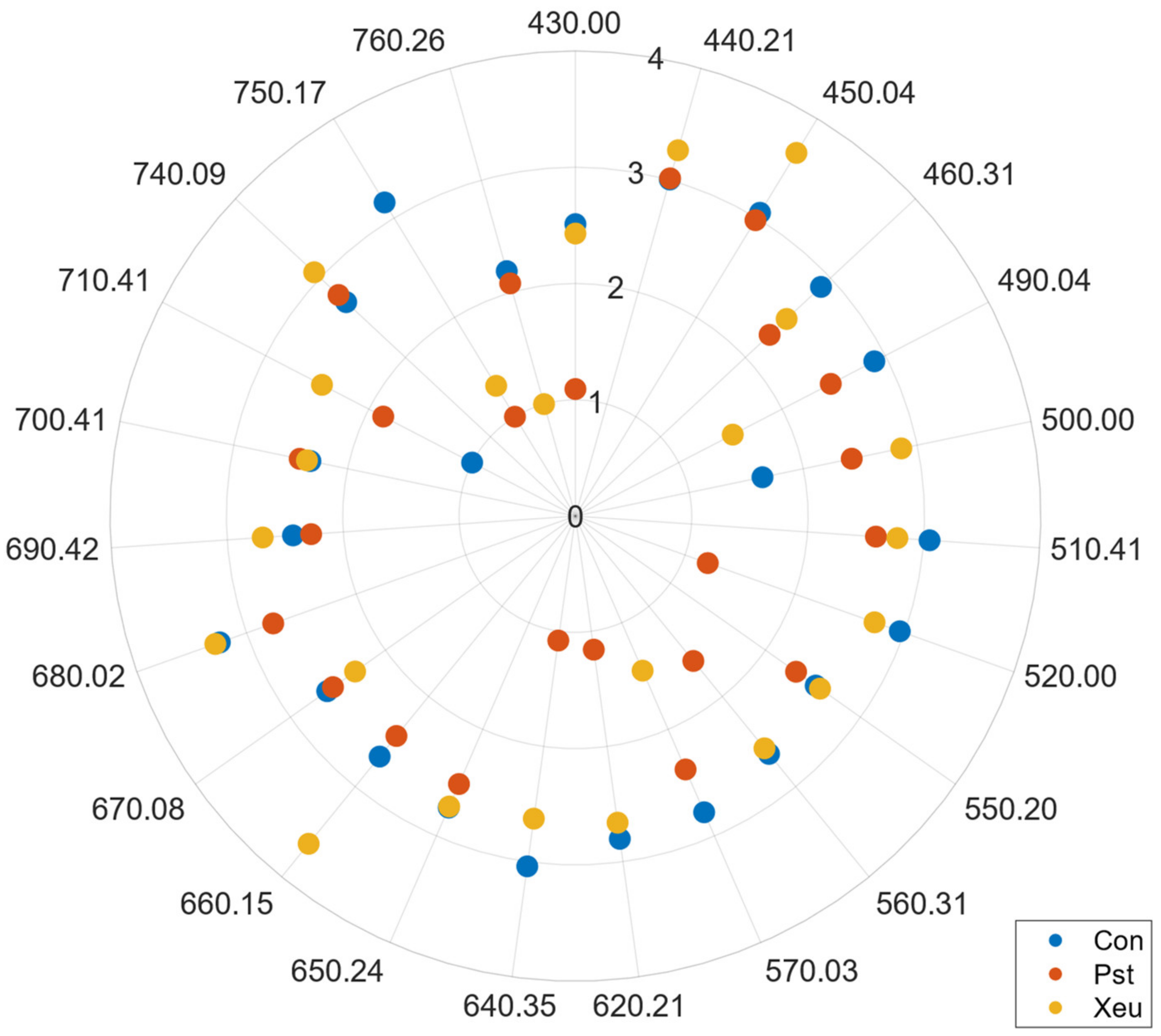
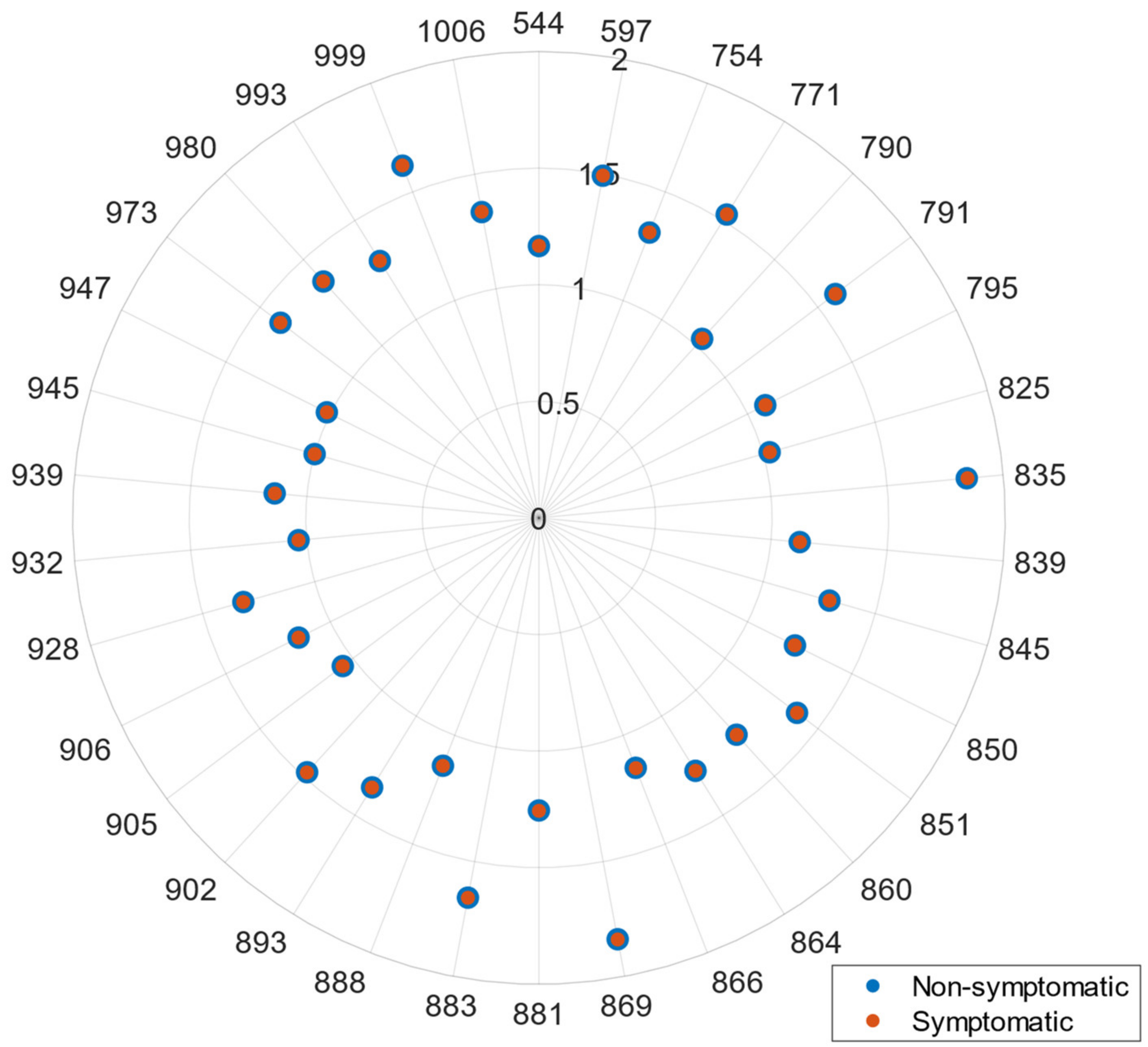
In this regard, Feature Selection or spectral reduction techniques are, thus, recommended to overcome this hurdle. In this work, two approaches were analyzed namely an FDA algorithm and the BAT of ARMO. Given the selected wavelengths, both studied strategies (VI-based vs. GPC-BAT) presented comparable results for both case studies, notably when dealing with the more complex tomato dataset especially with the tomato dataset. Equivalent wavelengths were found in the blue (450 nm), green (550 nm), and red-edge regions (680, 690, 700, and 750 nm). VIs further highlighted the 800 nm wavelength in the NIR region. In the kiwi case study, the features selected by the two algorithms were similar but not entirely coincident, namely in the green region (where VIs selected the 530, 553, and 554 nm, and the GPC-BAT chosen the 544, 597 nm), red-edge region (Vis identified the 670, 677, 700, 705, 730, and 750 nm as relevant, and GPC-BAT only considered the 754 nm), and NIR region (Vis picked a lower amount of wavelengths, namely 780, 800, 994, and 1000 nm, when compared to the GPC-BAT which took into account the following wavelengths 771, 790, 791, 795, 825, 835, 839, 845, 850, 851, 860, 864, 866, 869, 881, 883, 888, 893, 902, 905, 906, 928, 932, 939, 945, 947, 973, 980, 993, 999, and 1006 nm). Only the Vis presented features in the blue region 400 and 450 nm. Thus, it is important to address that despite the two modeling strategies applied to work with different types of spectra (reflectance vs. transmittance), having different spectral resolution (~10–10 nm vs. 1–1 nm) and presenting different pre-processing methods, they selected similar wavelengths.

These findings present biological significance, since the relationship between the plant host and the pathogen causes changes in photosynthetic pigment content, water levels, and structural composition (e.g., cellulose and lignin levels) [92]. This ultimately leads to modifications in the tissues’ spectral behavior. In particular, the variance in spectral characteristics among diseased leaves infected by distinct bacteria could be linked to the generation of unique molecules by each pathogen, which may influence the spectral signature of the host. For instance, Pst bacteria produce a specific phytotoxin named coronatine that induces changes in chlorophyll fluorescence (by altering photosystem II—PSII), impacting tomato plant tissues’ absorption and scattering of light [93]. Moreover, the host tomato plant can activate diverse defense responses upon encountering a pathogen, initiating a cascade of biochemical and molecular reactions that further contribute to spectral modifications in the visible wavelength ranges. Phytoalexins (e.g., flavonoids) serve as an example, with their production hypothesized to be linked to an increase in the spectral reflectance of plants in the VIS range [94].

Previous studies performed by our team also reported similar outcomes. In particular, that study developed a methodology for early diagnosing two bacterial diseases of tomato, caused by Pst and Xeu bacteria, using hyperspectral transmittance data and an applied predictive modeling approach [19]. A total of 3478 spectral measurements were normalized and subjected to a Linear Discriminant Analysis (LDA) aiming to reduce data dimensionality. This algorithm highlighted similar relevant wavelengths in the blue, green, and red spectral regions. Furthermore, a modeling approach using a Support Vector Machine was applied for spectral classification. It achieved an accuracy of 100% for samples measured on tissues inoculated with Pst and 74% for tissues inoculated with Xeu when samples collected before symptom appearance were used [19]. Likewise, another study performed on a kiwi orchard allowed the identification of hyperspectral reflectance samples collected on nonsymptomatic and symptomatic Psa disease leaf tissues. Several methodologies involving different Feature Selection techniques combined with different Machine Learning algorithms were explored, and the one combining a stepwise forward various selection (SFVS) approach followed by the computation of an SVM algorithm was selected, achieving an overall accuracy of 85%. Similar to the other strategies explored, the SFVS elected the blue region, green region, and NIR region as the most relevant for sample classification.

Furthermore, other researchers reported similar classification findings to the ones found in the present work, namely when studying different tomato and kiwi diseases based on modeling hyperspectral spectroscopy data. The suitability of a portable hyperspectral spectrometer combined with various algorithms for FS and data modeling for early nondestructive diagnosis of tomato bacterial wilt disease (Erwinia tracheiphila) in leaves was explored [95]. The model presenting higher evaluation metrics (overall accuracy of 90.70%) applied Genetic Algorithms for FS and SVM to predict classification. The Simple Ratio Pigment Index (SRPI) was the VI and was found to have a higher contribution in the developed model. It considers 430 and 680 nm wavelengths and is sensitive to leaf nitrogen content and photosynthetic efficiency (and is similar to our findings) [95].

Another study using tomato plants explored the usage of a portable high-resolution spectroradiometer combined with VIs, Principal Component Analysis (PCA), and a classification model K-nearest neighbor (KNN) for the diagnosis of late blight (Phytophthora infestans), target (Corynespora cassiicola), and bacterial spot (Xanthomonas euvesicatoria) [96]. They successfully identified the spectral samples collected on detached tomato leaflets with an accuracy reaching the 100% level even in nonsymptomatic stages (Error Rate of 9.50%), when the 15 VIs selected by PCA in the first principal component (PC) were considered. Interestingly, it is possible to observe that when 30 VIs selected by PCA and belonging to the first PC were used, the model showed a lower accuracy value (65.20%) and a higher error rate (28.6). In terms of VIs, the ones selected presented similar features to the ones found in our study (such as the 680 and 800 nm used in the Normalized difference index and the Simple Ratio, and structure-intensive pigment index, among others) [96].

Hyperspectral VIS-NIR spectroscopy was, moreover, used for the nondestructive early diagnosis of tomato chlorosis virus (ToCV) [97]. They used a Neighborhood component analysis (NCA) for performing FS and for selecting the most relevant VIs in the study, along with two ML models for data modeling (XY-fusion network—XY-F—and Multilayer Perceptron with Automated Relevance Determination—MLP-ARD). The best overall accuracy (92.1% before outlier removal and 100% after outlier removal) was obtained using MLP-ARD. In terms of relevant VIs, is possible to observe that wavelengths such as 550, 670, 700, 720, 740, and 800 nm, among others, were present in the most notable VIs formulae (such as Anthocyanin Reflectance Index—ARI, Pigment Specific Simple Ratio—PSSR, Red Edge Inflection Point—REIP, Simple Ratio—SR, and Vogelmann Index—VOG). In turn, from the 15 wavelengths selected by the NCA, these were mostly located in the blue (402.20 to 449.20 nm), green (556.40 to 566.40 nm), red-edge (676.40 to 726.30 nm), and NIR regions (862.10 nm). These outcomes coincided with our observations [97].

The feasibility of multispectral data for predicting kiwifruit decline (probably caused by Phytophtora spp. and Phytopythium spp.) in diseased orchards was also tested [98]. Multispectral data included the 550, 660, and 790 nm spectral features, and when combined with K-means clustering allowed the determination of kiwi plants’ vigor affected or not by the disease with 73% (or more) Accuracy and 82% Precision. These results are, thus, in line with ours also identifying the green, red, and NIR regions as relevant for estimating plant biophysical traits [98].

The present outcomes demonstrate that hyperspectral transmittance and reflectance spectroscopy can identify healthy and diseased tissues, such as tomato (herbaceous) and kiwi (woody) crops, in laboratory or field conditions. Further research is advised to explore if specific host–pathogen interactions require customized modeling approaches to be predicted or if it is possible to elaborate a unified strategy that allows bacterial disease assessment. Nevertheless, it should be taken into consideration that model comparison may be challenging due to several factors: pathogen species in the study; the occurrence of specific host–pathogen interactions; the number of spectral points measured; the environmental conditions where the data are collected; and the stage of the disease cycle where the spectral assessments are made, among others. Furthermore, hyperspectral spectroscopy sensors present a relatively low Technology Readiness Level (TRL), indicating that these sensors have a large margin to be improved. In this regard, developing and enhancing effective FS strategies or Dimensionality Reduction approaches may be conducted to identify specific spectral regions valuable for performing plant disease diagnosis, which may be incorporated in multispectral sensors involving lower production and data processing costs. Moreover, the application of hyperspectral imaging sensors should also be explored in future studies, since it would offer a comprehensive spectral overview across spatial dimensions, allowing the capture of spectral signatures from several pixels in the image. This spatial information enables the identification of spatial variations in spectral features within the plant tissue sample, which can provide valuable insights into the spatial distribution of disease symptoms or other physiological changes. However, hyperspectral imaging typically requires more complex data processing and may involve higher equipment costs compared to point-measurement techniques, which must be taken into consideration in the technique development.

5. Conclusions

This study aimed to explore and compare two distinct modeling approaches, namely the parametric Spectral Vegetation Indices (VIs) and the Gaussian Process Classification based on an Automated Spectral Band Analysis Tool (GPC-BAT), for diagnosing bacterial diseases in plants using hyperspectral sensing. Our analysis covered two experimental conditions, namely controlled conditions where tomato plants were used and field conditions where kiwi plants were analyzed, revealing insights into the performances of each approach.

Both the VI- and GPC-BAT-based approaches demonstrated potential for class discrimination in both experiments. Nevertheless, the modeling strategy applying VIs showed moderate success in distinguishing healthy and Pst-inoculated tomato tissues, with accuracy values ranging from 63% to 71%. In turn, the GPC-BAT strategy exhibited enhanced accuracy in classifying healthy and diseased tissues, achieving overall accuracy values extending from 70% to 75% in the tomato and kiwi case studies. This approach also revealed greater potential for discriminating nonsymptomatic from symptomatic tissues in kiwi plants in field conditions.

The identified spectral bands, particularly in the blue, green, red-edge, and NIR regions, align with the absorption regions of several photosynthetic pigments and plant structural components. These spectral modifications correlate with bacterial infections, affecting chlorophylls, carotenoids, flavonoids, pheophytins, and water content in plant leaves.

Hence, while VIs offer a simplistic yet moderately effective means of disease diagnosis, GPC-BAT, with feature reduction, shows promise in improving accuracy. However, further refinements are necessary, especially for the early-stage diagnosis of specific bacterial infections.

The identified wavelengths hold biological significance, suggesting a correlation between bacterial infections and alterations in photosynthetic pigments and leaf structural components. Future research could focus on refining and integrating these approaches to develop more robust and accurate diagnostic tools for various plant–pathogen interactions, thereby aiding in early disease detection and management in diverse agricultural settings.

References

1. Ristaino, J.B.; Anderson, P.K.; Bebber, D.P.; Brauman, K.A.; Cunniffe, N.J.; Fedoroff, N.V.; Finegold, C.; Garrett, K.A.; Gilligan, C.A.; Jones, C.M.; et al. The persistent threat of emerging plant disease pandemics to global food security. Proc. Natl. Acad. Sci. USA 2021, 118, e2022239118. [Google Scholar] [CrossRef] [PubMed]
2. Martinelli, F.; Scalenghe, R.; Davino, S.; Panno, S.; Scuderi, G.; Ruisi, P.; Villa, P.; Stroppiana, D.; Boschetti, M.; Goulart, L.R. Advanced methods of plant disease detection. A review. Agron. Sustain. Dev. 2015, 35, 1–25. [Google Scholar] [CrossRef]
3. Dyussembayev, K.; Sambasivam, P.; Bar, I.; Brownlie, J.C.; Shiddiky, M.J.A.; Ford, R. Biosensor technologies for early detection and quantification of plant pathogens. Front. Chem. 2021, 9, 636245. [Google Scholar] [CrossRef] [PubMed]
4. Zhang, J.C.; Huang, Y.B.; Pu, R.L.; Gonzalez-Moreno, P.; Yuan, L.; Wu, K.H.; Huang, W.J. Monitoring plant diseases and pests through remote sensing technology: A review. Comput. Electron. Agric. 2019, 165, 104943. [Google Scholar] [CrossRef]
5. Mahlein, A.K.; Oerke, E.C.; Steiner, U.; Dehne, H.W. Recent advances in sensing plant diseases for precision crop protection. Eur. J. Plant Pathol. 2012, 133, 197–209. [Google Scholar] [CrossRef]
6. Jacquemoud, S.; Baret, F. PROSPECT: A model of leaf optical properties spectra. Remote Sens. Environ. 1990, 34, 75–91. [Google Scholar] [CrossRef]
7. Jensen, J.R. REMOTE Sensing of the Environment: An earth Resource Perspective 2/e. 2009: Pearson Education India. Available online: https://www.academia.edu/2969968/Remote_Sensing_of_the_Environment_An_Earth_Resource_Perspective_2_e (accessed on 1 January 2024).
8. Sahoo, R.N.; Ray, S.S.; Manjunath, K.R. Hyperspectral Remote sensing of agriculture. Curr. Sci. 2015, 108, 848–859. [Google Scholar]
9. Jones, H.G.; Vaughan, R.A. Remote Sensing of Vegetation: Principles, Techniques, and Applications; Oxford University Press: Oxford, UK, 2010. [Google Scholar]
10. Deshmukh, R.; Janse, P.; Karungaru, S.; Kalyankar, N.; Koinkar, P. Hyperspectral Remote Sensing for Agriculture: A Review. 2018. Available online: https://www.researchgate.net/profile/Ratnadeep-Deshmukh-2/publication/325295759_Hyperspectral_Remote_Sensing_for_Agriculture_A_Review/links/5b041f6eaca2720ba09972f5/Hyperspectral-Remote-Sensing-for-Agriculture-A-Review.pdf (accessed on 1 January 2024).
11. Haq, I.U.; Ijaz, S. Plant Disease Management Strategies for Sustainable Agriculture through Traditional and Modern Approaches; Springer International Publishing: New York, NY, USA, 2020. [Google Scholar]
12. Galieni, A.; D’Ascenzo, N.; Stagnari, F.; Pagnani, G.; Xie, Q.G.; Pisante, M. Past and future of plant stress detection: An overview from Remote Sensing to Positron Emission Tomography. Front. Plant Sci. 2021, 11, 609155. [Google Scholar] [CrossRef]
13. Thomas, S.; Kuska, M.T.; Bohnenkamp, D.; Brugger, A.; Alisaac, E.; Wahabzada, M.; Behmann, J.; Mahlein, A.-K. Benefits of hyperspectral imaging for plant disease detection and plant protection: A technical perspective. J. Plant Dis. Prot. 2018, 125, 5–20. [Google Scholar] [CrossRef]
14. Szymańska, E. Modern data science for analytical chemical data—A comprehensive review. Anal. Chim. Acta 2018, 1028, 1–10. [Google Scholar] [CrossRef]
15. Verrelst, J.; Malenovský, Z.; Van der Tol, C.; Camps-Valls, G.; Gastellu-Etchegorry, J.-P.; Lewis, P.; North, P.; Moreno, J. Quantifying vegetation biophysical variables from Imaging Spectroscopy data: A review on retrieval methods. Surv. Geophys. 2019, 40, 589–629. [Google Scholar] [CrossRef] [PubMed]
16. Mahlein, A.K.; Rumpf, T.; Welke, P.; Dehne, H.W.; Plümer, L.; Steiner, U.; Oerke, E.C. Development of spectral indices for detecting and identifying plant diseases. Remote Sens. Environ. 2013, 128, 21–30. [Google Scholar] [CrossRef]
17. Verrelst, J.; Rivera, J.P.; Veroustraete, F.; Muñoz-Marí, J.; Clevers, J.G.P.W.; Camps-Valls, G.; Moreno, J. Experimental Sentinel-2 LAI estimation using parametric, non-parametric and physical retrieval methods—A comparison. ISPRS J. Photogramm. Remote Sens. 2015, 108, 260–272. [Google Scholar] [CrossRef]
18. Verrelst, J.; Rivera, J.P.; Gitelson, A.; Delegido, J.; Moreno, J.; Camps-Valls, G. Spectral band selection for vegetation properties retrieval using Gaussian processes regression. Int. J. Appl. Earth Obs. Geoinf. 2016, 52, 554–567. [Google Scholar] [CrossRef]
19. Reis Pereira, M.; Santos, F.N.D.; Tavares, F.; Cunha, M. Enhancing host-pathogen phenotyping dynamics: Early detection of tomato bacterial diseases using hyperspectral point measurement and predictive modeling. Front. Plant Sci. 2023, 14, 1242201. [Google Scholar] [CrossRef]
20. Reis Pereira, M.; Tavares, F.; Santos, F.; Cunha, M. Hyperspectral Spectroscopic Transmittance Data Collected In-Vivo Healthy and Diseased Tomato Leaflets in Controlled Conditions-Dataset II; Zenodo: Genève, Switzerland, 2024. [Google Scholar]
21. Reis-Pereira, M.; Tosin, R.; Martins, R.; Santos, F.N.D.; Tavares, F.; Cunha, M. Kiwi plant canker diagnosis using hyperspectral signal processing and Machine Learning: Detecting symptoms caused by Pseudomonas syringae pv. actinidiae. Plants 2022, 11, 2154. [Google Scholar] [CrossRef]
22. Stefani, E.; Loreti, S. PM 7/120 (1) Pseudomonas syringae pv. actinidiae. Bull. OEPP 2014, 44, 360–375. [Google Scholar]
23. Mariz-Ponte, N.; Gimranov, E.; Rego, R.; Moura, L.; Santos, C.; Tavares, F. Distinct phenotypic behaviours within a clonal population of Pseudomonas syringae pv. actinidiae. PLoS ONE 2022, 17, e0269343. [Google Scholar] [CrossRef]
24. Reis Pereira, M.; Tavares, F.; Santos, F.; Cunha, M. Hyperspectral Spectroscopic Reflectance Data Collected In-Vivo Non-Symptomatic and Symptomatic Kiwi Leaves in Field Conditions; Zenodo: Genève, Switzerland, 2024. [Google Scholar]
25. Tosin, R.; Martins, R.; Pocas, I.; Cunha, M. Canopy VIS-NIR spectroscopy and self-learning artificial intelligence for a generalised model of predawn leaf water potential in Vitis vinifera. Biosyst. Eng. 2022, 219, 235–258. [Google Scholar] [CrossRef]
26. Asner, G.P. Biophysical and biochemical sources of variability in canopy reflectance. Remote Sens. Environ. 1998, 64, 234–253. [Google Scholar] [CrossRef]
27. Verdebout, J.; Jacquemoud, S.; Schmuck, G. Optical properties of leaves: Modelling and experimental studies. In Imaging Spectrometry—A Tool for Environmental Observations; Hill, J., Mégier, J., Eds.; Springer: Dordrecht, The Netherlands, 1994; pp. 169–191. [Google Scholar]
28. Lang, M.; Stober, F.; Lichtenthaler, H.K. Fluorescence emission spectra of plant leaves and plant constituents. Radiat. Environ. Biophys. 1991, 30, 333–347. [Google Scholar] [CrossRef] [PubMed]
29. Hennessy, A.; Clarke, K.; Lewis, M. Hyperspectral classification of plants: A review of waveband selection generalisability. Remote Sens. 2020, 12, 113. [Google Scholar] [CrossRef]
30. Moriya, É.A.S.; Imai, N.N.; Tommaselli, A.M.G.; Honkavaara, E.; Rosalen, D.L. Design of Vegetation Index for identifying the mosaic virus in sugarcane plantation: A Brazilian case study. Agronomy 2023, 13, 1542. [Google Scholar] [CrossRef]
31. Gitelson, A.; Merzlyak, M.N. Quantitative estimation of chlorophyll-a using reflectance spectra: Experiments with autumn chestnut and maple leaves. J. Photochem. Photobiol. B Biol. 1994, 22, 247–252. [Google Scholar] [CrossRef]
32. Blackmer, T.M.; Schepers, J.S.; Varvel, G.E. Light reflectance compared with other nitrogen stress measurements in corn leaves. Agron. J. 1994, 86, 934–938. [Google Scholar] [CrossRef]
33. Lichtenthaler, H.K.; Gitelson, A.; Lang, M. Non-destructive determination of chlorophyll content of leaves of a green and an aurea mutant of tobacco by reflectance measurements. J. Plant Physiol. 1996, 148, 483–493. [Google Scholar] [CrossRef]
34. Haboudane, D.; Miller, J.R.; Pattey, E.; Zarco-Tejada, P.J.; Strachan, I.B. Hyperspectral vegetation indices and novel algorithms for predicting green LAI of crop canopies: Modeling and validation in the context of precision agriculture. Remote Sens. Environ. 2004, 90, 337–352. [Google Scholar] [CrossRef]
35. Henrich, V.; Götze, E.; Jung, A.; Sandow, C.; Thürkow, D.; Gläßer, C. Development of an online indices database: Motivation, concept and implementation. In Proceedings of the 6th EARSeL Imaging Spectroscopy Sig Workshop Innovative Tool for Scientific and Commercial Environment Applications, Tel Aviv, Israel, 16–19 March 2009. [Google Scholar]
36. Henrich, V.; Krauss, G.; Götze, C.; Sandow, C. Index Data Base a Database for Remote Sensing Indices. 2023. Available online: https://www.indexdatabase.de/ (accessed on 3 January 2024).
37. Lantz, B. Machine Learning with R: Expert Techniques for Predictive Modeling; Packt Publishing Ltd.: Birmingham, UK, 2019. [Google Scholar]
38. Kuhn, M.; Johnson, K. Applied Predictive Modeling; Springer: Berlin/Heidelberg, Germany, 2013; Volume 26. [Google Scholar]
39. Reis-Pereira, M.; Tosin, R.; Martins, R.C.; Santos, F.N.D.; Tavares, F.; Cunha, M. Enhancing kiwi bacterial canker leaf assessment: Integrating hyperspectral-based Vegetation Indexes in predictive modeling. Eng. Proc. 2023, 48, 22. [Google Scholar]
40. Team, R.C. R: A Language and Environment for Statistical Computing. 2021. Available online: https://apps.dtic.mil/sti/citations/ADA612335 (accessed on 3 January 2024).
41. Kuhn, M. Caret: Classification and Regression Training. Astrophysics Source Code Library. 2015, p. ascl: 1505.003. Available online: https://www.ascl.net/1505.003 (accessed on 1 January 2024).
42. Milborrow, M.S. Package ‘Earth’, version 2.4-8; R Software Package; Citeseer: Princeton, NJ, USA, 2019. [Google Scholar]
43. Ashburn, P. The Vegetative Index Number and Crop Identification; NASA. Johnson Space Center Proc. of Tech. Sessions: Houston, TX, USA, 1979; Volume 1–2. [Google Scholar]
44. Bannari, A.; Morin, D.; Bonn, F.; Huete, A. A review of vegetation indices. Remote Sens. Rev. 1995, 13, 95–120. [Google Scholar] [CrossRef]
45. Gitelson, A.A.; Merzlyak, M.; Zur, Y.; Stark, R.; Gritz, U. Non-Destructive and Remote Sensing Techniques for Estimation of Vegetation Status. In Proceedings of the 3rd European Conference on Precision Agriculture, Montpelier, France, 18–20 June 2001. [Google Scholar]
46. Merzlyak, M.; Gitelson, A.; Chivkunova, O.; Solovchenko, A.; Pogosyan, S. Application of reflectance spectroscopy for analysis of higher plant pigments. Russ. J. Plant Physiol. 2003, 50, 704–710. [Google Scholar] [CrossRef]
47. Zarco-Tejada, P.J.; Berjón, A.; López-Lozano, R.; Miller, J.R.; Martín, P.; Cachorro, V.; González, M.R.; de Frutos, A. Assessing vineyard condition with hyperspectral indices: Leaf and canopy reflectance simulation in a row-structured discontinuous canopy. Remote Sens. Environ. 2005, 99, 271–287. [Google Scholar] [CrossRef]
48. Barnes, E.M.; Clarke, T.R.; Richards, S.E.; Colaizzi, P.D.; Haberland, J.; Kostrzewski, M.; Waller, P.; Choi, C.R.E.; Thompson, T.; Lascano, R.J.; et al. Coincident detection of crop water stress, nitrogen status and canopy density using ground based multispectral data. In Proceedings of the Fifth International Conference on Precision Agriculture, Bloomington, MN, USA, 16 July 2000. [Google Scholar]
49. Henrich, V.; Krauss, G.; Götze, C.; Sandow, C. The Index Database. 2012. Available online: https://www.indexdatabase.de/ (accessed on 3 January 2024).
50. Clarke, T.R.; Moran, M.S.; Barnes, E.M.; Pinter, P.J., Jr.; Qi, J. Planar domain indices: A method for measuring a quality of a single component in two-component pixels. In Proceedings of the IGARSS 2001, Scanning the Present and Resolving the Future, IEEE 2001 International Geoscience and Remote Sensing Symposium (Cat. No.01CH37217), Sydney, Australia, 6 August 2002; pp. 1279–1281. [Google Scholar]
51. Pinter, P.J.; Hatfield, J.L.; Schepers, J.S.; Barnes, E.M.; Moran, M.S.; Daughtry, C.S.T.; Upchurch, D.R. Remote sensing for crop management. Photogramm. Eng. Remote Sens. 2003, 69, 647–664. [Google Scholar] [CrossRef]
52. El-Shikha, D.M.; Barnes, E.M.; Clarke, T.R.; Hunsaker, D.J.; Haberland, J.A.; Pinter, P.J.; Waller, P.M.; Thompson, T.L. Remote sensing of cotton nitrogen status using the Canopy Chlorophyll Content Index (CCCI). Trans. Asabe 2008, 51, 73–82. [Google Scholar] [CrossRef]
53. Herrmann, I.; Karnieli, A.; Bonfil, D.J.; Cohen, Y.; Alchanatis, V. SWIR-based spectral indices for assessing nitrogen content in potato fields. Int. J. Remote Sens. 2010, 31, 5127–5143. [Google Scholar] [CrossRef]
54. Gitelson, A.A.; Keydan, G.P.; Merzlyak, M.N. Three-band model for noninvasive estimation of chlorophyll, carotenoids, and anthocyanin contents in higher plant leaves. Geophys. Res. Lett. 2006, 33, 11. [Google Scholar] [CrossRef]
55. Escadafal, R.; Belghith, A.; Ben Moussa, H. Indices spectraux pour la télédétection de la dégradation des milieux naturels en Tunisie aride. In Proceedings of the 6th International Symposium on Physical Measurements and Signatures in Remote Sensing, Val D’Isere, France, 17–21 January 1994. [Google Scholar]
56. Ahamed, T.; Tian, L.; Zhang, Y.; Ting, K. A review of remote sensing methods for biomass feedstock production. Biomass Bioenergy 2011, 35, 2455–2469. [Google Scholar] [CrossRef]
57. Gitelson, A.A.; Viña, A.; Arkebauer, T.J.; Rundquist, D.C.; Keydan, G.; Leavitt, B. Remote estimation of leaf area index and green leaf biomass in maize canopies. Geophys. Res. Lett. 2003, 30, 1248. [Google Scholar] [CrossRef]
58. Hunt, E.R., Jr.; Daughtry, C.; Eitel, J.U.; Long, D.S. Remote sensing leaf chlorophyll content using a visible band index. Agron. J. 2011, 103, 1090–1099. [Google Scholar] [CrossRef]
59. Datt, B.; McVicar, T.R.; Van Niel, T.G.; Jupp, D.L.; Pearlman, J.S. Preprocessing EO-1 Hyperion hyperspectral data to support the application of agricultural indexes. IEEE Trans. Geosci. Remote Sens. 2003, 41, 1246–1259. [Google Scholar] [CrossRef]
60. Le Maire, G.; François, C.; Dufrene, E. Towards universal broad leaf chlorophyll indices using PROSPECT simulated database and hyperspectral reflectance measurements. Remote Sens. Environ. 2004, 89, 1–28. [Google Scholar] [CrossRef]
61. Main, R.; Cho, M.A.; Mathieu, R.; O’Kennedy, M.M.; Ramoelo, A.; Koch, S. An investigation into robust spectral indices for leaf chlorophyll estimation. ISPRS J. Photogramm. Remote Sens. 2011, 66, 751–761. [Google Scholar] [CrossRef]
62. Huete, A.; Didan, K.; Miura, T.; Rodriguez, E.P.; Gao, X.; Ferreira, L.G. Overview of the radiometric and biophysical performance of the MODIS vegetation indices. Remote Sens. Environ. 2002, 83, 195–213. [Google Scholar] [CrossRef]
63. Gitelson, A.A.; Kaufman, Y.J.; Merzlyak, M.N. Use of a green channel in remote sensing of global vegetation from EOS-MODIS. Remote Sens. Environ. 1996, 58, 289–298. [Google Scholar] [CrossRef]
64. Wang, F.-M.; Huang, J.-F.; Tang, Y.-L.; Wang, X.-Z. New vegetation index and its application in estimating leaf area index of rice. Rice Sci. 2007, 14, 195–203. [Google Scholar] [CrossRef]
65. Pinty, B.; Verstraete, M. GEMI: A non-linear index to monitor global vegetation from satellites. Vegetatio 1992, 101, 15–20. [Google Scholar] [CrossRef]
66. Zarco-Tejada, P.J.; Miller, J.R.; Noland, T.L.; Mohammed, G.H.; Sampson, P.H. Scaling-up and model inversion methods with narrow-band optical indices for chlorophyll content estimation in closed forest canopies with hyperspectral data. IEEE Trans. Geosci. Remote Sens. 2001, 39, 1491–1507. [Google Scholar] [CrossRef]
67. Lee, W.S.; Alchanatis, V.; Yang, C.; Hirafuji, M.; Moshou, D.; Li, C. Sensing technologies for precision specialty crop production. Comput. Electron. Agric. 2010, 74, 2–33. [Google Scholar] [CrossRef]
68. Schlerf, M.; Atzberger, C.; Hill, J. Remote sensing of forest biophysical variables using HyMap imaging spectrometer data. Remote Sens. Environ. 2005, 95, 177–194. [Google Scholar] [CrossRef]
69. Crippen, R.E. Calculating the vegetation index faster. Remote Sens. Environ. 1990, 1, 71–73. [Google Scholar] [CrossRef]
70. Kooistra, L.; Leuven, R.S.E.W.; Wehrens, R.; Nienhuis, P.H.; Buydens, L.M.C. A comparison of methods to relate grass reflectance to soil metal contamination. Int. J. Remote Sens. 2003, 24, 4995–5010. [Google Scholar] [CrossRef]
71. Misra, P.N.; Wheeler, S.G.; Oliver, R.E. Kauth-Thomas Brigthness and Greenness Axes; Contract NASA: Washington, DC, USA, 1977; pp. 23–46. [Google Scholar]
72. Huete, A.R.; Liu, H.Q.; Batchily, K.; van Leeuwen, W. A comparison of vegetation indices over a global set of TM images for EOS-MODIS. Remote Sens. Environ. 1997, 59, 440–451. [Google Scholar] [CrossRef]
73. Chen, J.M. Evaluation of vegetation indices and a modified simple ratio for boreal applications. Can. J. Remote Sens. 1996, 22, 229–242. [Google Scholar] [CrossRef]
74. Thenkabail, P.S.; Smith, R.B.; De Pauw, E. Evaluation of narrowband and broadband vegetation indices for determining optimal hyperspectral wavebands for agricultural crop characterization. Photogramm. Eng. Remote Sens. 2002, 68, 607–621. [Google Scholar]
75. Zarco-Tejada, P.J.; Sepulcre-Cantó, G. Remote Sensing of Vegetation Biophysical Parameters for Detecting Stress Condition and Land Cover Changes. Estudios de la Zona No Saturada del Suelo. Vol. VIII. J.V. Giráldez Cervera y F.J. Jiménez Hornero. 2007. Available online: https://zonanosaturada.com/zns07/publications_files/inv/04.pdf (accessed on 1 January 2024).
76. Apan, A.; Held, A.; Phinn, S.; Markley, J. Formulation and assessment of narrow-band vegetation indices from EO-1 hyperion imagery for discriminating sugarcane disease. In Proceedings of the 2003 Spatial Sciences Institute Conference: Spatial Knowledge without Boundaries (SSC2003), Canberra, Australia, 22–26 September 2003; pp. 1–13. [Google Scholar]
77. Sims, D.A.; Gamon, J.A. Relationships between leaf pigment content and spectral reflectance across a wide range of species, leaf structures and developmental stages. Remote Sens. Environ. 2002, 81, 337–354. [Google Scholar] [CrossRef]
78. Clevers, J.; De Jong, S.; Epema, G.; Van Der Meer, F.; Bakker, W.; Skidmore, A.; Scholte, K. Derivation of the red edge index using the MERIS standard band setting. Int. J. Remote Sens. 2002, 23, 3169–3184. [Google Scholar] [CrossRef]
79. Verrelst, J.; Romijn, E.; Kooistra, L. Mapping vegetation density in a heterogeneous river floodplain ecosystem using pointable CHRIS/PROBA data. Remote Sens. 2012, 4, 2866–2889. [Google Scholar] [CrossRef]
80. Hubert-Moy, L.; Cotonnec, A.; Le Du, L.; Chardin, A.; Pérez, P. A comparison of parametric classification procedures of remotely sensed data applied on different landscape units. Remote Sens. Environ. 2001, 75, 174–187. [Google Scholar] [CrossRef]
81. Phiri, D.; Morgenroth, J. Developments in Landsat land cover classification methods: A review. Remote Sens. 2017, 9, 967. [Google Scholar] [CrossRef]
82. Rasmussen, C.E.; Williams, C.K. Gaussian Processes for Machine Learning; Springer: Berlin/Heidelberg, Germany, 2006; Volume 1. [Google Scholar]
83. Schölkopf, B.; Smola, A.; Müller, K.-R. Nonlinear component analysis as a kernel eigenvalue problem. Neural Comput. 1998, 10, 1299–1319. [Google Scholar] [CrossRef]
84. Bishop, C.M.; Nasrabadi, N.M. Pattern Recognition and Machine Learning; Springer: Berlin/Heidelberg, Germany, 2006; Volume 4. [Google Scholar]
85. Aghababaei, M.; Ebrahimi, A.; Naghipour, A.A.; Asadi, E.; Pérez-Suay, A.; Morata, M.; Garcia, J.L.; Rivera Caicedo, J.P.; Verrelst, J. Introducing ARTMO’s Machine-Learning Classification Algorithms Toolbox: Application to plant-type detection in a semi-steppe Iranian landscape. Remote Sens. 2022, 14, 4452. [Google Scholar] [CrossRef]
86. Bazi, Y.; Melgani, F. Toward an optimal SVM classification system for hyperspectral remote sensing images. IEEE Trans. Geosci. Remote Sens. 2006, 44, 3374–3385. [Google Scholar] [CrossRef]
87. Archibald, R.; Fann, G. Feature selection and classification of hyperspectral images with support vector machines. IEEE Geosci. Remote Sens. Lett. 2007, 4, 674–677. [Google Scholar] [CrossRef]
88. Pal, M.; Foody, G.M. Feature selection for classification of hyperspectral data by SVM. IEEE Trans. Geosci. Remote Sens. 2010, 48, 2297–2307. [Google Scholar] [CrossRef]
89. Zhang, F.; Yang, X. Improving land cover classification in an urbanized coastal area by random forests: The role of variable selection. Remote Sens. Environ. 2020, 251, 112105. [Google Scholar] [CrossRef]
90. Caicedo, J.P.R.; Verrelst, J.; Muñoz-Marí, J.; Moreno, J.; Camps-Valls, G. Toward a semiautomatic machine learning retrieval of biophysical parameters. IEEE J. Sel. Top. Appl. Earth Obs. Remote Sens. 2014, 7, 1249–1259. [Google Scholar] [CrossRef]
91. Rivera, J.P.; Verrelst, J.; Delegido, J.; Veroustraete, F.; Moreno, J. On the semi-automatic retrieval of biophysical parameters based on spectral index optimization. Remote Sens. 2014, 6, 4927–4951. [Google Scholar] [CrossRef]
92. Blancard, D. 3—Principal Characteristics of Pathogenic Agents and Methods of Control, in Tomato Diseases, 2nd ed.; Blancard, D., Ed.; Academic Press: San Diego, CA, USA, 2012; pp. 413–650. [Google Scholar]
93. Zhang, Z.; He, B.; Sun, S.; Zhang, X.; Li, T.; Wang, H.; Xu, L.; Afzal, A.J.; Geng, X. The phytotoxin COR induces transcriptional reprogramming of photosynthetic, hormonal and defence networks in tomato. Plant Biol. 2021, 23, 69–79. [Google Scholar] [CrossRef] [PubMed]
94. Leucker, M.; Wahabzada, M.; Kersting, K.; Peter, M.; Beyer, W.; Steiner, U.; Mahlein, A.-K.; Oerke, E.-C. Hyperspectral imaging reveals the effect of sugar beet quantitative trait loci on Cercospora leaf spot resistance. Funct. Plant Biol. 2016, 44, 1–9. [Google Scholar] [CrossRef]
95. Cen, Y.; Huang, Y.; Hu, S.; Zhang, L.; Zhang, J. Early detection of bacterial wilt in tomato with portable Hyperspectral Spectrometer. Remote Sens. 2022, 14, 2882. [Google Scholar] [CrossRef]
96. Lu, J.; Ehsani, R.; Shi, Y.; de Castro, A.I.; Wang, S. Detection of multi-tomato leaf diseases (late blight, target and bacterial spots) in different stages by using a spectral-based sensor. Sci. Rep. 2018, 8, 2793. [Google Scholar] [CrossRef]
97. Morellos, A.; Tziotzios, G.; Orfanidou, C.; Pantazi, X.E.; Sarantaris, C.; Maliogka, V.; Alexandridis, T.K.; Moshou, D. Non-destructive early detection and quantitative severity stage classification of Tomato Chlorosis Virus (ToCV) infection in young tomato plants using Vis–NIR Spectroscopy. Remote Sens. 2020, 12, 1920. [Google Scholar] [CrossRef]
98. Savian, F.; Martini, M.; Ermacora, P.; Paulus, S.; Mahlein, A.-K. Prediction of the kiwifruit decline syndrome in diseased orchards by Remote Sensing. Remote Sens. 2020, 12, 2194. [Google Scholar] [CrossRef]
Figure 1. Experimental setup of the bacterial inoculation assay performed on tomato leaves (walk-in experimental conditions), and in kiwi leaves (field experimental conditions). In both cases, spectral measurements were performed on the adaxial side of the leaves. In the tomato case study, they were, furthermore, performed on the 4th, 5th, and 6th leaves of the assay plants, in a dark room, using a spectrometer (measuring transmittance data) combined with an optical fiber bundle with a reflection probe. A white LED was placed beneath each leaflet. In kiwi, spectra collection was performed in random points of leaves casually selected, using a passive spectroradiometer (measuring reflectance data).
Agronomy 14 00493 g001
Figure 2. Conceptual framework for the predictive modeling approaches of bacterial diseases of tomato and kiwi.
Agronomy 14 00493 g002
Figure 3. Schematic flow diagram of GPC-BAT within ARTMO’s MLCA toolbox, adapted from [18].
Agronomy 14 00493 g003
Figure 4. Gaussian Process Classification sigma bands polar plot, representing the most significant wavelengths for each class in the study: Control samples (healthy, Con), samples inoculated with Pseudomonas syringae pv. tomato (Pst), and samples inoculated with Xanthomonas euvesicatoria (Xeu). The lower the sigma value, the greater the importance of the wavelength.
Agronomy 14 00493 g004
Figure 5. Gaussian Process Classification sigma bands polar plot, representing the most significant wavelengths for the binary class in the study: nonsymptomatic (NS) and symptomatic (S). The lower the sigma value, the greater the importance of the wavelength.
Agronomy 14 00493 g005