Designing an Economical Water Harvesting System Using a Tank with Numerical Simulation Model WASH_2D

Abstract

Newly incorporated module into the WASH_2D model has enabled simulating a rainwater harvesting system (RWHS) using a tank. The incorporated module in WASH_2D was tested for two field experiments to determine the optimal tank capacity and cultivated area that give the highest net income for farmers. The first experiment was composed of treatments A, B, and C having the same cultivated and harvested areas (plastic sheets) of 24 m² and 12.5 m², respectively. The capacity of the tanks for treatments A, B, and C was set at 500, 300, and 200 L, corresponding to storability of 21, 13, and 8 mm, respectively, while in the second experiment we carried out three treatments: F, G, and H having the same tank capacity of 300 L and harvested area of 12.5 m² with variable cultivated areas as G and H were larger by two and three times than F (10.5 m²), respectively. Water was applied automatically through a drip irrigation system by monitoring soil water suction. Results of the first experiment showed that the optimal storability and seasonal net income simulated by WASH_2D were 17 mm and 5.82 USD yr⁻¹, which were fairly close to 18 mm and 5.75 USD yr⁻¹ observed from field data, respectively. Similarly, the results of the second experiment revealed that simulated net incomes for different cultivated areas agreed well with the observed data. We concluded that the use of the simulation model WASH_2D can be economically useful to promote small-scale irrigation in semi-arid regions and guide planning irrigation or rainwater harvesting investments.

1. Introduction

In dryland farming, drought stress has been one of the most serious environmental factors that causes significant crop failures. Therefore, the use of supplemental irrigation (SI) could avoid crop failure and improve yield and farmer financial income [1,2,3,4,5,6]. In places away from irrigation canals and having no irrigation infrastructure, the application of SI in rainfed agriculture can be enhanced through the construction of rainwater harvesting systems (RWHS). The RWHS was defined as a system to harvest rainfall runoff from a catchment area, store it in a reservoir, and use it to irrigate normally-rainfed crops for a long time when rainfall alone is not enough to provide soil moisture in the root zone to support crop growth and enhance plant development [7].The typical RWHS consists of a catchment area that can be a plastic sheet as an example, reservoir (e.g., polyethylene tanks), and irrigation network (e.g., drip irrigation system). These systems can be more efficient if they are incorporated with automated irrigation systems, which can wisely respond to provide soil moisture deficits in the crop root zone [7,8]. The common RWHS include unlined soil reservoirs [1,9], lined soil reservoirs [3,10,11] and tanks [12,13,14,15]. One of the critical limitations of the unlined and lined soil reservoirs is low storage efficiency. In unlined soil reservoirs, much water is often lost through seepage and deep percolation. In a lined soil reservoir without cover, loss of harvested water is still uncontrolled due to evaporation. Therefore, the use of tanks (i.e., lined and covered reservoirs) in RWHS can overcome those shortcomings of other systems. However, the storage capacity or the economical design of the RWHS is still an important issue for farmers [15,16,17,18]. Construction cost and high seepage rates have been the major limitations of storage water in soil reservoirs for SI [19,20]. In sandy soil where runoff is limited, seepage losses can be greater than 25 mm day⁻¹ [5]. Instead of harvesting rainwater in earth reservoirs, plastic or concrete tanks can be utilized to improve the effectiveness of rainwater storage. The tank, for example, can be prefabricated, taking less time to install than standard ones. In hilly sites with poor access to irrigation canals and infrastructure, the use of tanks for SI may enhance food and water security in rainfed farming based on the lifetime of the tank materials. The energy consumption for SI may be reduced if water is supplied by gravity using the advantages of slopes in hilly sites.

In sandy soil where runoff is limited, the use of plastic sheets or solar panels as catchment areas may enhance the storage tank efficiency because the runoff ratio of them is 100%. Designing an economical RWHS using a tank is important to stabilize crop production in rainfed areas where canals are not accessible and groundwater is very deep or too saline. The optimal design of tank capacity should not depend only on crop water requirements but also on maximizing net income. The larger the tank we install, the greater the chance of storing water we may have, while the larger the cost we must cover. In addition, large-cultivated areas in a RWHS will increase agricultural inputs such as labor, fertilizers, SI, and crop seeds, whereas smaller cultivated areas may enhance water applied, but the total yield will be lower. A proper design of an economical RWHS for SI is complex, and therefore few attempts to properly optimize the storage reservoir for dissemination of the practice have been made. Verma and Sarma [21] presented a numerical scheme for designing storage tanks for water harvesting for SI. Moreover, the reliability of the method depends on the basis of the lowest assured runoff for pre-sowing irrigation, whereas Srivastava [19] developed a simulation model for determining catchment/cultivated area ratio (CCR) and the size of the tank using water balance in the reservoir. A linear programming optimization model combining with a watershed modeling system was developed by Al-Ansari et al. [22] to determine the optimal cultivated area and the optimal reservoir capacity that meet the crop water demand. Shinde et al. [23] presented an algorithm for sizing reservoirs for rainwater harvesting and SI, using a multi-reservoir model for Water Harvesting and Supplementary Irrigation System for Cascaded reservoirs in a watershed (WH-SIS-CAD), while Mishra et al. [16] developed a multi-objective optimization model to determine the optimal size of the storage reservoir area. Traore and Wang [24] designed the surface reservoir to be constructed from the total cultivated area based on water balance in the reservoir and supplemental irrigation using a simulation flowchart. Recently, Vico et al. [25] proposed a numerical model for designing a farm reservoir for SI to enhance and stabilize yields. The model required monitoring soil moisture, the change in storage depth, and crop biomass. The focus of those trails was to either maximize irrigated area on a large scale or minimize the costs of tank capacity per unit of available water. However, they have not taken into account the response of the crop to the SI-based rain harvest, and they have not linked the optimal tank design with either productivity or crop water demand. Few of them have employed simple water balance calculations to incorporate the crop water demand. A numerical model presented by Pandey et al. [26] used the change in water in the soil reservoir and the water balance in the field to find the optimal size of the storage reservoir.

The use of numerical simulation models for soil water flow and crop response to irrigation (HYDRUS [27], SWAP [28], or WASH_2D [29]) should be incorporated into designing and simulating RWHS. However, none of them has employed numerical simulations of water flow in soils and root water uptake, although accuracy in prediction of water flow and root water uptake is critical for proper evaluation of the response of rain and irrigation on crop yield. A new module was developed and incorporated into WASH_2D [29] to simulate RWHS for SI using tanks. The module can simulate automated irrigation and limitations of tank capacity for the automated simulation. It can also simulate storage in the tank, considering runoff efficiency and loss rate owing to leakage, seepage, or evaporation.

The objective of this study was firstly to evaluate the accuracy of the optimal capacity using WASH_2D with that observed in the field in a water harvesting using a plastic sheet and tank. The second objective was to compare the simulated net income using WASH_2D with the one in the field under three different sizes of cultivated area in a water harvesting using plastic sheet and tank.

2. Materials and Methods

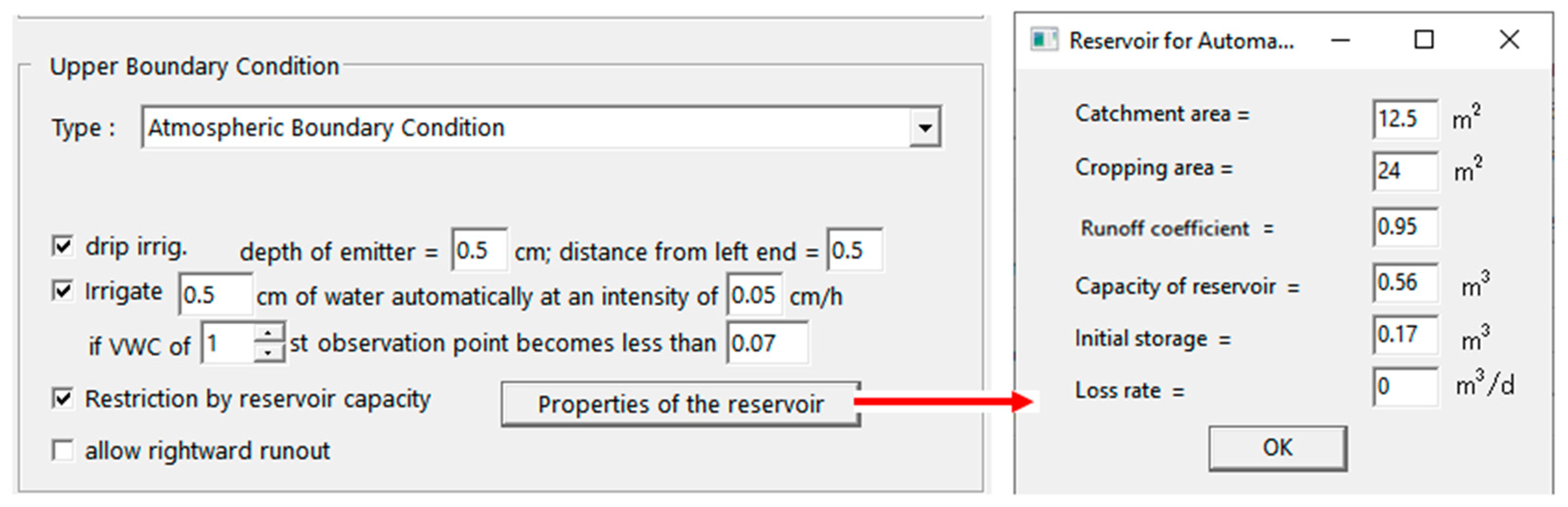
2.1. Numerical Model, WASH_2D

The WASH_2D model [29] simulates two-dimensional movement of water, solute, and heat in the soil with the alternative direction finite difference method. The model solves the two-dimensional water conservation equation of the combined liquid and gaseous phases using Richard’s equation as:

$${\displaystyle \frac{\partial \mathsf{\theta }}{\partial \mathrm{t}}}=-\langle {\displaystyle \frac{{\partial \mathrm{q}}_{\mathrm{l}\mathrm{x}}}{\partial \mathrm{x}}}+{\displaystyle \frac{{\partial \mathrm{q}}_{\mathrm{l}\mathrm{z}}}{\partial \mathrm{z}}}\rangle -\langle {\displaystyle \frac{{\partial \mathrm{q}}_{\mathrm{v}\mathrm{x}}}{\partial \mathrm{x}}}+{\displaystyle \frac{{\partial \mathrm{q}}_{\mathrm{v}\mathrm{z}}}{\partial \mathrm{z}}}\rangle +S$$

(1)

where t is time (h); $q_l$ and $q_v$ are respectively liquid water flux (cm h⁻¹) and water vapor flux (cm h⁻¹); x and z are horizontal distance and depth (cm), respectively; and where $S$ is root water uptake rate (h⁻¹), which is described by the macroscopic root water uptake model [30] as follows.

$$S=\mathsf{\alpha }{T}_{rp}\mathsf{\beta }$$

(2)

where $S$ is root water uptake rate (h⁻¹); $T_{rp}$ is the potential transpiration rate (cm h⁻¹); β is the normalized root density or root activity (cm⁻¹); and $\mathsf{\alpha }$ is a reduction coefficient so-called, stress response function (SRF), which is calculated as a function of matrices and osmotic potentials:

$$\mathsf{\alpha }={\displaystyle \frac{1}{1+{\left(\frac{h}{h_{50}}+\frac{h_o}{h_{o50}}\right)}^p}}$$

(3)

where $h$ and $h_o$ are the matric and osmotic heads, respectively; $h_{50}$ and $h_{o50}$ are the matric and osmotic potentials when the water uptake is 50% of its potential rate; and $p$ is an empirical parameter.

The values of these fitting parameters were using the approach described by Yanagawa and Fujimaki [31].

The $\mathsf{\beta }$ is described as:

$$\mathsf{\beta }=0.75 \left(b_{rt}+1\right){d_{rt}}^{-b_{rt}-1}({d_{rt}-z+z_{r0})}^{b_{rt}} g_{rt}(1-x^2{g_{rt}}^{-2})$$

(4)

where $b_{rt}$ is a fitting parameter; $d_{rt}$ and $g_{rt}$ are the depth and the width of the plant root zone (cm), respectively; $z$ and $z_{r0}$ are the soil depth and the depth below which roots exist (cm), respectively, $x$ is the is the horizontal distance from the plant (cm).

The $d_{rt}$ is expressed as a function of cumulative transpiration, τ, from germination as follows:

$$d_{rt}=a_{d_{rt}}\left[1-exp\left(b_{d_{rt}}\tau \right)\right]+c_{d_{rt}}$$

(5)

where $a_{d_{rt}}$, $b_{d_{rt}}$, and $c_{d_{rt}}$ are fitting parameters.

The $T_{rp}$ is calculated by multiplying reference evapotranspiration (${ET}_0$) by basal crop coefficient ($K_{cb}$) using the approach of FAO 56 [32].

$$K_{cb}=k_{cb}=a_{L_{AI}}\left[1-\mathrm{e}\mathrm{x}\mathrm{p}\left(b_{L_{AI}}\tau \right)\right]+c_{k_{cb}}-d_{k_{cb}}{\tau }^{{e_k}_{cb}}$$

(6)

where ${\mathrm{a}}_{{\mathrm{L}}_{\mathrm{A}\mathrm{I}}}, {\mathrm{b}}_{{\mathrm{L}}_{\mathrm{A}\mathrm{I}}}, {\mathrm{c}}_{{\mathrm{k}}_{\mathrm{c}\mathrm{b}}}, \mathrm{a}\mathrm{n}\mathrm{d} {\mathrm{d}}_{{\mathrm{k}}_{\mathrm{c}\mathrm{b}}}$ are fitting parameters. This equation was used to estimate the $K_{cb}$ until the end of the mid-season. In late stage, the $K_{cb}$ is calculated as a function of day to physiological maturity. The methodology for determining the fitting parameter values of $d_{rt}$ and $K_{cb}$ were described by [29].

The model employs the thermal properties of the soil, including the dependency of the thermal conductivity and albedo of the water content. Thermal conductivity, $k_h$ (W cm⁻¹ K⁻¹) was estimated as:

$$k_h=a_h+b_h\left({\displaystyle \frac{\theta }{{\theta }_{sat}}}\right)-(a_h-d_h)exp\left[-c_h{\left({\displaystyle \frac{\theta }{{\theta }_{sat}}}\right)}^{e_h}\right]$$

(7)

where ${\theta }_{sat}$ is saturated $\theta$; $a_h$, $b_h$, $c_h$, $d_h$, and $e_h$ are fitting parameters. While albedo, ${\alpha }_R,$ was estimated as:

$${\alpha }_R={\displaystyle \frac{{\alpha }_{max}-{\alpha }_{min}}{1+{\left(a_{al}\overline{\theta }\right)}^{b_{al}}}}+{\alpha }_{min}$$

(8)

where ${\alpha }_{max}, {\alpha }_{min}$, $a_{al}$ and $b_{al}$ are fitting parameters.

2.2. Simulation of RWHS in WASH_2D

A new module was developed to evaluate the effect of limitation of tank capacity in a RWHS using tanks on SI, which was incorporated into the WASH 2D model (Figure 1). The model presents an impermeable tank to store the harvested rainwater from a catchment area. SI water is applied from the tank to the cultivated area via an automatic irrigation system. Irrigation water was applied to plants at a rate based on rain and prediction of root water uptake due to drought ($h_{50}$, p) or salinity (${ho}_{50}, p)$ stress. Note that the software is flexible and allows the user to enter the different parameters of the RWHS (Figure 1), such as the size of the catchment area, the cultivated area, the storage capacity, or the runoff efficiency.

Losses owing to seepage and evaporation can also be considered, but in this study, it was set at zero because polyethylene tanks did not allow seepage losses and evaporation. When the tank is filled to its capacity, any inflow to the tank is lost through overflow. The crop yield, Y (kg m⁻²) over the growing season was assumed to be proportional to the cumulative transpiration. The predicted transpiration rate from the WASH_2D model was used to calculate the yield as follows:

$$Y={10ϵ}_{T}HI\sum T_{rp}$$

(9)

where ${ϵ}_T$ is the transpiration productivity (dimensionless) and $HI$ is the harvest index (%) and $\sum T_{rp}$ is the cumulative transpiration (cm) (1 cm = 10 kg m⁻² of water).

2.3. Optimization of Tank Capacity in RWHS

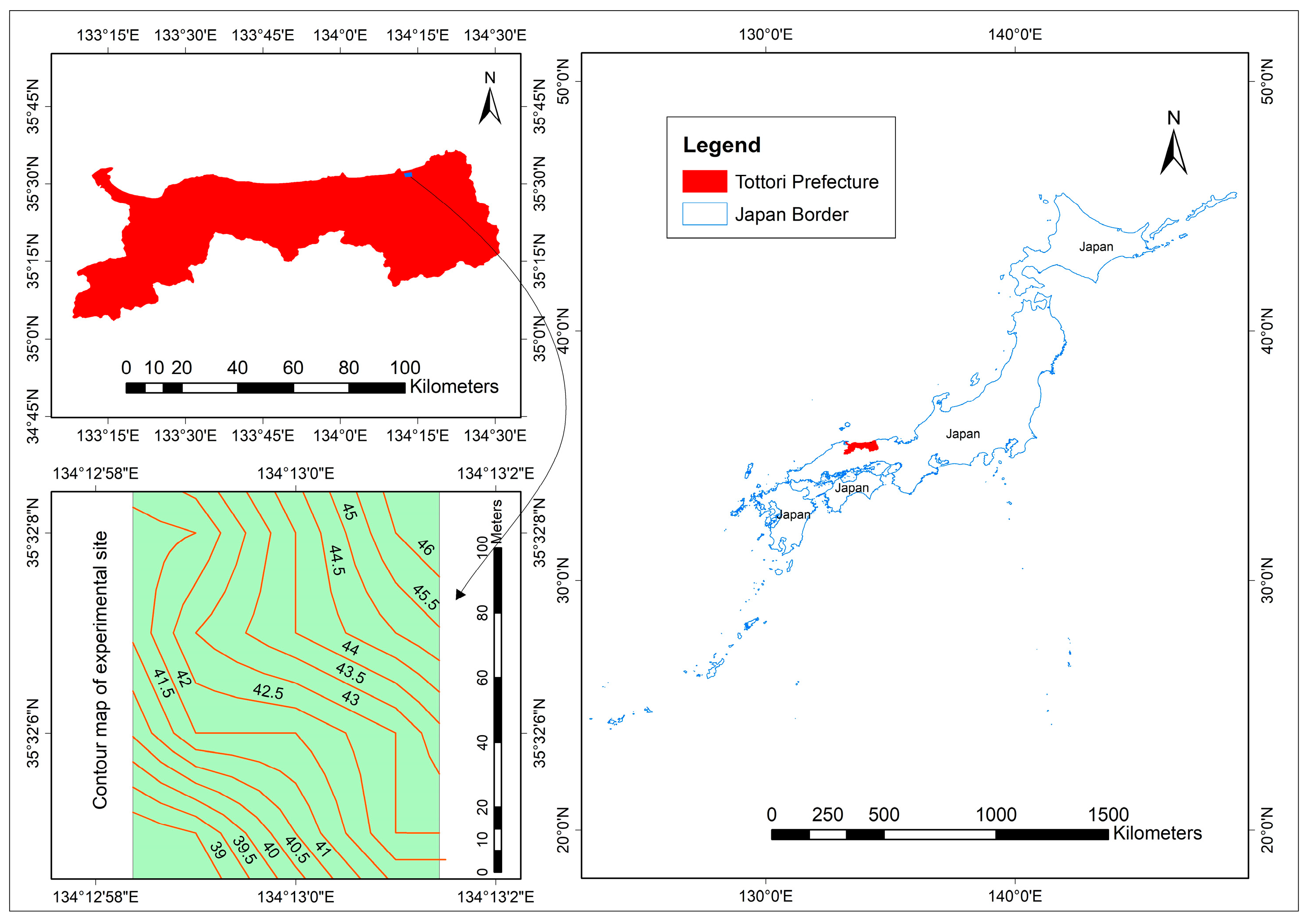
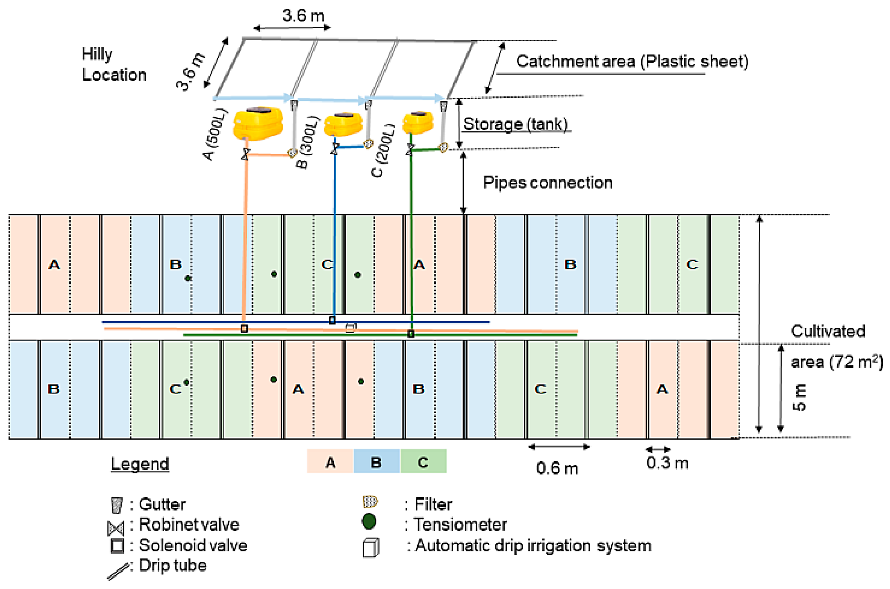
2.3.1. Field Experiment 1

The experiment was carried out on a sand dune in the Arid Land Research Center, Japan (Figure 2). The field experiment consisted of three treatments: A, B, and C having the same cultivated area of 24 m² but different polyethylene tank capacities of 500, 300, and 200 L, with corresponding storability (storage capacity divided by cultivated area) of 21, 13, and 8 mm, respectively (Figure 3). Each treatment had the same area of plastic sheet (3.6 m × 3.6 m) as the catchment area installed on a slope of 15 degrees. Rainwater was harvested from the plastic sheets and conveyed to the storage tanks using a combination of a gutter, filter, and piping system. Water was applied by gravity using an automated drip irrigation system. The emitters and laterals were spaced at 20 and 60 cm, respectively. Water was applied for each treatment when the average observed suction of the two tensiometers installed at the depth of 20 cm exceeded a trigger value of 50 cm. Irrigation was controlled using a CR1000 data logger (Campbell Scientific, Inc., Logan, UT, USA) and solenoid valves.

Garlic cloves were sown in two rows along each drip on 30 September 2021. The distances between plants along drip tubes and between rows were 13.3 cm and 16 cm, respectively. 110 kg ha⁻¹ of N from N-P-K fertilizer of 8-8-8 in solid form was applied three times, 46, 70, and 117 days after sowing, while 160 kg ha⁻¹ of liquid fertilizer N-P-K from composite 8-10-5 was applied to all treatments after two weeks of transplanting. A weather station was set up on the fields. The cumulative rainfall across the growing season was 873 mm.

To evaluate the net income, we set the cost of tanks at 2.6, 2.2, and 1.7 USD yr⁻¹ for treatments A, B, and C, respectively, by considering the 30-year life span. The cost of plastic sheet and drip irrigation were not included because the plastic sheet mimicked solar panels, which do not require any cost if they already exist, and the cost of drip irrigation may be negligible if it is properly maintained.

The producer price of garlic bulbs was set at 1.6 USD kg⁻¹ and the total cost of cultivation, including the cost of seeds, was 0.08 USD m⁻². The net income, $I_n$, (USD yr⁻¹) due to the application of SI can be estimated as follows:

$$I_n=P_{c}Y-C_T$$

(10)

where $P_c$ is the price of crop (USD kg⁻¹); and $Y$ is the total yield (kg yr⁻¹), $C_T$ is the total cost of cultivation (USD yr⁻¹). The optimal storability, $x$, which is the ratio between storage capacity and cultivated area, is achieved at maximum $I_n$ by determining the fitting parameters of a parabola function as:

$$I_n=a{\left(x-x_{max}\right)}^2+I_{n_{max}}$$

(11)

where $a$, $x_{max}$ and $I_{n_{max}}$ are fitting parameters. Note that the value of parameter $a$ is always negative; therefore, $x_{max}$ represents the optimal storability which gives maximum net income, $I_{n_{max}}$.

2.3.2. Procedure of Numerical Optimization of Tank Capacity

The simulation was performed for each treatment: A, B, and C, from sowing to harvesting date that spans 230 days. The irrigation was set to be automatically applied at a rate of 0.05 cm h⁻¹ using drip irrigation with an emitter depth of 0.5 cm at an irrigation depth of 5 mm when the trigger value reached 0.07. The upper boundary condition was set at atmospheric conditions, and the left boundary condition was set as impermeable, while the lower boundary condition was set as gravitational flow. The maximal volumes of harvested water observed in the field in treatments A, B, and C were 560, 330, and 220 L, respectively, owing to overflow from the gutters. The catchment areas and cultivated areas were set at the same values of 12.5 m² and 24 m², respectively. The initial storage water amounts in tanks A, B, and C were 170, 100, and 60 L, respectively. The runoff ratios (k_r) used in the model for A, B, and C were 95, 85, and 50%, respectively. The initial transpiration rate was set at 0.5 cm. The plant rows were located 8 cm apart on both sides of the drip tube. We ran the simulation twice successively at 125 and 105 days for each treatment. The daily simulation started at 9:00 AM from 13 October 2021 until the harvest of garlic bulbs.

2.4. Net Income for RWHS with Different Cultivated Areas

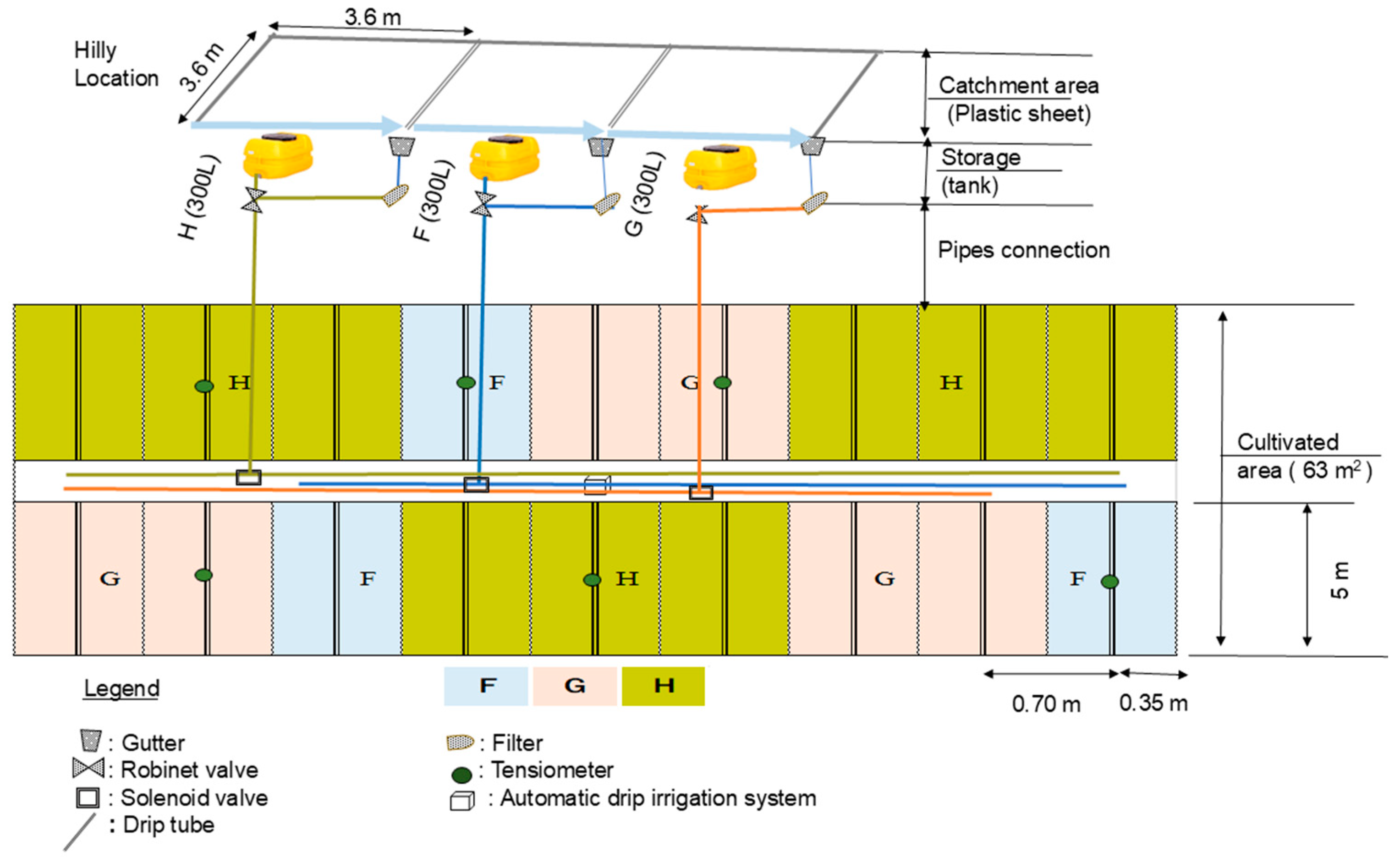
2.4.1. Field Experiment 2

In a sandy field close to the location of the garlic experiment, we set up three treatments: F, G, and H having the same tank capacity of 300 L and the same catchment area (plastic sheet of 3.6 m × 3.6 m), installed on a slope of 15 degrees. The treatments had different cultivated areas of 10.5, 21, and 31.5 m², respectively. The irrigation system with RWHS was identical to that of the garlic experiment (Figure 4). The differences were the lateral spacing of the drip irrigation system and the setting of trigger suction values, which were 70 cm and 45 cm, respectively. Irrigation was controlled using two CR300 data loggers (Campbell Scientific, Inc., Logan, UT, USA) and solenoid valves.

Mung bean seeds were sown under each emitter on 20 June 2023. We followed standard cultivation management and fertilizer application for mung beans. The experiment was terminated on 28 September 2023, and six samples in each replicated treatment were collected once the crops were fully matured under the prevalent conditions to measure the yield on 9 October 2023.

To calculate the $I_n$, we set the cost of tank at 7 USD m⁻³ yr⁻¹. The producer price of mung bean seed was 10 USD kg⁻¹, and the total cost of cultivation, including the cost of seeds, was 0.025 USD m⁻². The measured I_n (USD yr⁻¹) due to the application of SI can be estimated using Equation (10).

2.4.2. Numerical Prediction of Net Income for the Experiment 2

The period of the simulation run was 97 days, equal to the period of 3 days after sowing to termination of the experiment. The irrigation was set to be automatically applied at a rate of 0.05 cm h⁻¹ using drip irrigation with an emitter depth of 0.5 cm at a depth of 5 mm when the trigger value reached 0.06. The upper boundary condition of the water flow was atmospheric, and both the left boundary and lower boundary conditions were set as impermeable. The lower boundary condition of the heat movement was set at zero temperature gradient. We observed the same maximal volume of harvested water of 330 L for each treatment F, G, and H. The catchment areas and cropping areas were the same values in the field experiment using the mung bean crop. For all tanks F, G, and H, the initial volume of storage water was zero. The runoff ratios (k_r) used in the simulation for F, G, and H were 60, 85, and 90%, respectively. The initial transpiration rate was set at 0.5 cm. The location of the plants was close to the emitter of the drip tube.

To calculate the simulated (Equation (9)) garlic bulb yield, we set the values of ${ϵ}_T$ and HI at 0.005 and 0.3, respectively, while that of mung bean, we set at 0.001 and 0.2. Both plant growth parameters used in the model WASH_2D were listed in

Table 1. Garlic and Mung-bean growth parameter values used in the model WASH_2D.

Parameter	Garlic		Mung-Bean
	Value		Remarks
h50	−50	[33]	−150	Equation (3)
ho50	−4821		−3300
p	27.5		2
b	1	Equation (4)	0.02	Equation (4)
grt	20		30
zr0	1		1
adrt	40		45
bdrt	−0.5		−0.5
cdrt	5	Equations (5) and (6)	5	Equations (5) and (6)
akc	0.87		1
bkc	−0.21		−0.15
ckc	0.15		0.1
tlate	200		78
tend	230		97
kcb	0.6		0.6
aLAI	2		2
bLAI	−0.02		−0.1

Note: Parameter values in Table 1 were obtained through the corresponding equation and fitted parameters using the corresponding equation described in a study by Fujimaki et al. [29].

.

Note that the soil used for simulation was Tottori sand, and the parameter values of the soil listed in

Table 2. Tottori sand parameters used in the numerical model WASH_2D.

Parameter	Value
θsat (cm3 cm−3)	0.42
θr (cm3 cm−3)	0.03
αv (cm−1)	0.018
n	4
${\mathit{a}}_{\mathit{h}}$	0.0061
${\mathit{b}}_{\mathit{h}}$	0.0032
${\mathit{c}}_{\mathit{h}}$	22.6
${\mathit{d}}_{\mathit{h}}$	0.00152
${\mathit{e}}_{\mathit{h}}$	1.46
${\mathit{\alpha }}_{\mathit{m}\mathit{a}\mathit{x}}$	0.224
${\mathit{\alpha }}_{\mathit{m}\mathit{i}\mathit{n}}$	0.159
${\mathit{a}}_{\mathit{a}\mathit{l}}$	8
${\mathit{b}}_{\mathit{a}\mathit{l}}$	3

were measured in the laboratory [29] using van Genuchten Equations (7) and (8). In both experiments, the climatic parameters data, such as precipitation intensity, weed speed, humidity, solar radiation, and air temperature, collected from the weather station installed in the field, was used as variable data in the model. The corresponding weather data, such as rainfall and air temperatures (Figure 5a,b), for each experiment showed a large change across the growing season. We corrected the intensity of the rainfall across the growing season for each to be uniform during heavy rain by reducing high precipitation intensity to improve the simulation running. The maximal rain intensity used in the model was 0.225 mm h⁻¹ for garlic experiments, while that for mung bean was set at 0.15 mm h⁻¹.

Although the total rain fell (873 mm) during the garlic growth period, we observed drought stress, and plants were supplementally irrigated due to the consumption of water in storage tanks [13]. Except for the snow period observed during garlic growth (Figure 5a). Both the climatic data observed indicate experimental conditions of a dryland climatic zone with high frequent drought spells in Figure 5b.

3. Results and Discussion

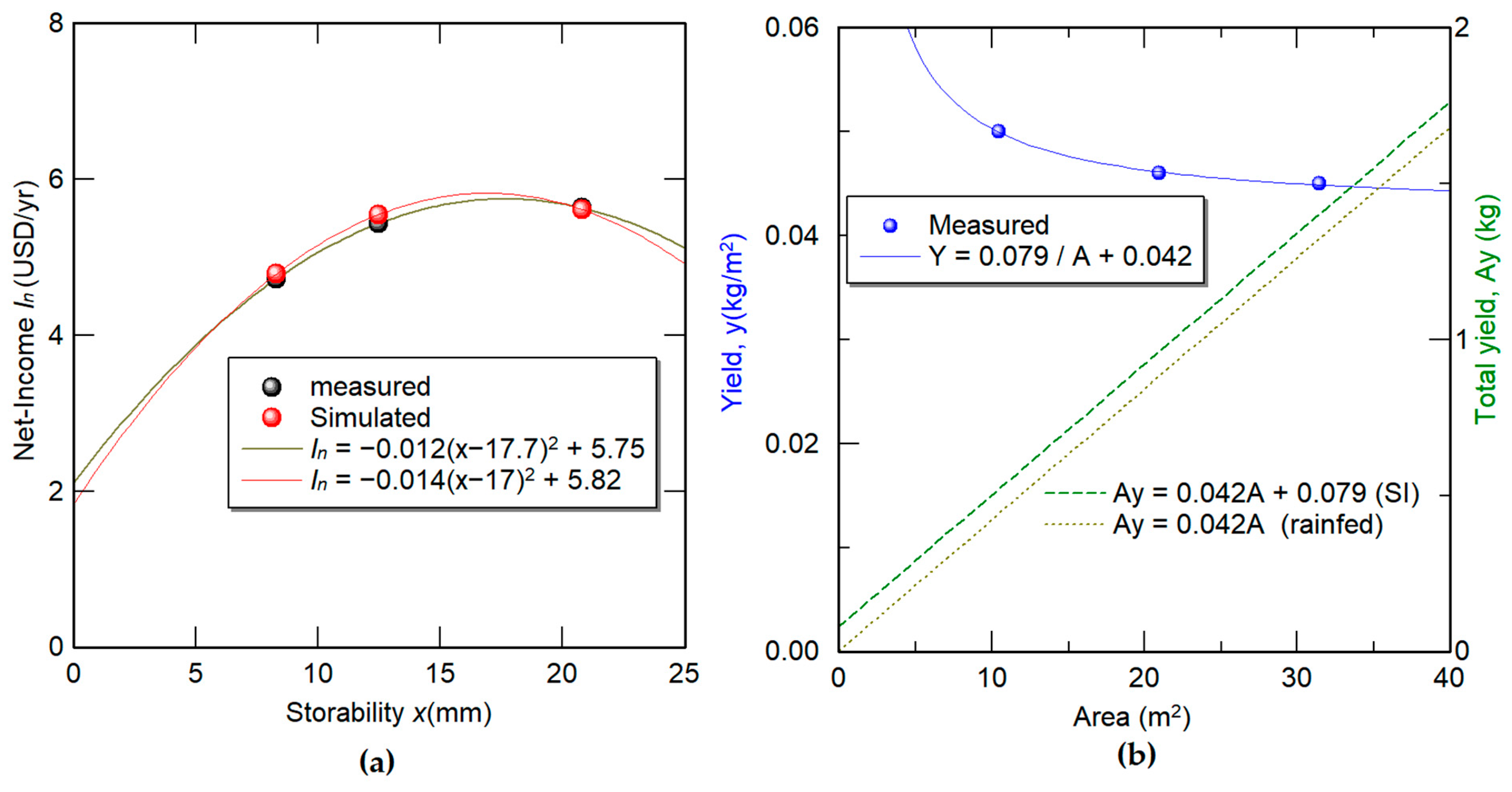
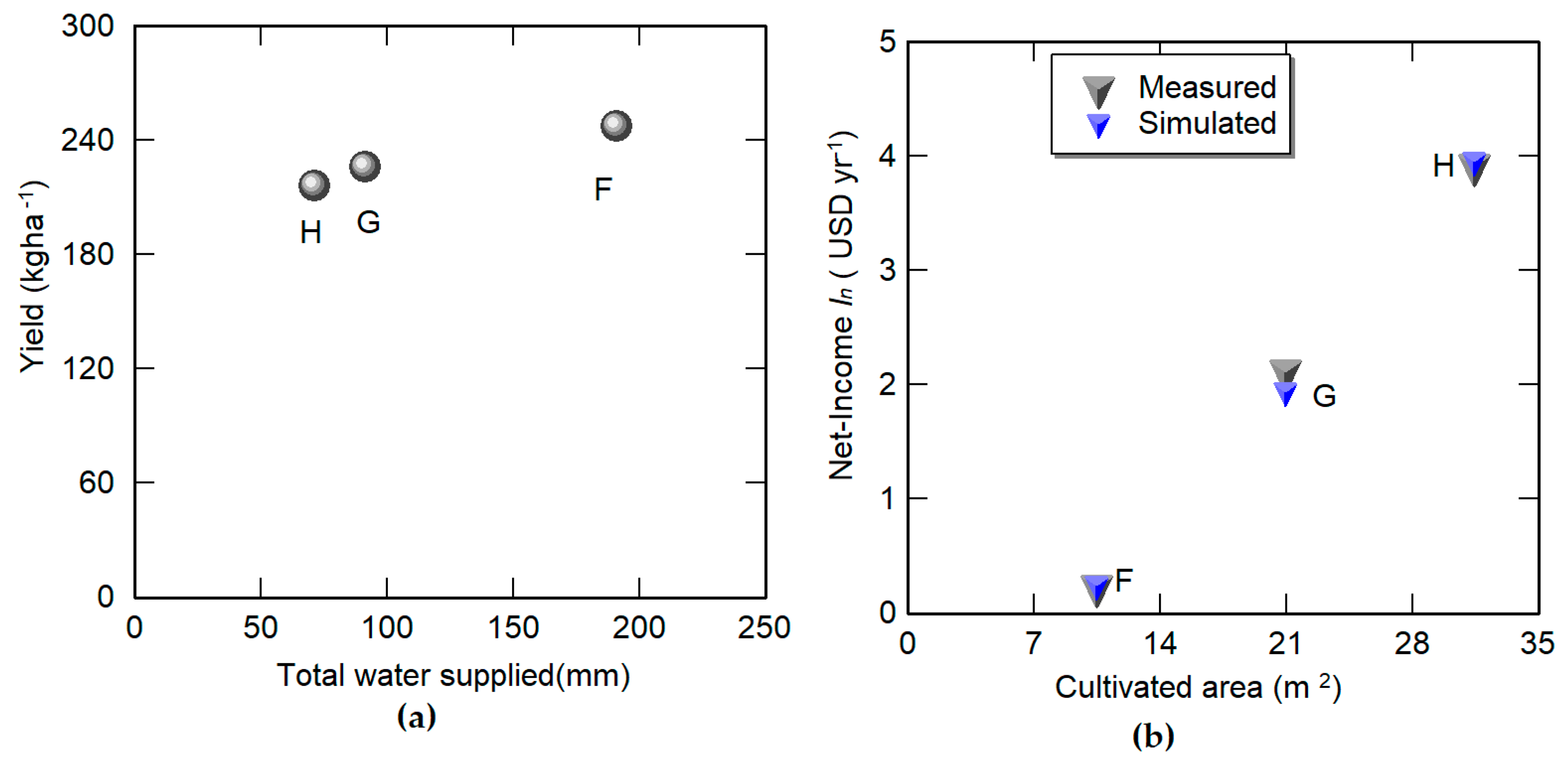
3.1. Optimization of Tank Capacity in Terms of $I_n$

A comparison between storability and both observed and simulated net income is shown in Figure 6a. The simulated bulb yields of A, B, and C were 6.4, 6.1, and 5.3 kg, respectively, close to the field observed data of 6.4, 6.0, and 5.3 kg, respectively. The observed $I_n$ was calculated by substituting the actual harvest yield into Equation (8), which was 5.6, 5.4, and 4.7 USD yr⁻¹ for A, B, and C, respectively, mean-while the simulated $I_n$ was 5.6, 5.5, and 4.8 USD yr⁻¹ for A, B, and C. Note that the simulated cumulative transpiration for A of 17.8 cm was higher than both B (16.9 cm) and C (14.7 cm). Those results were similar to the observed SI applied to A (74 cm), which was higher than both B (63 cm) and C (45 cm). The fitted curve of $I_n$ (Equation (9)) plotted in Figure 6a gave an optimal storability of 18 mm with maximum $I_{n_{max}}$.of 5.75 USD yr⁻¹ (1 USD = 140 JPY) [13], which was close to the simulated one of 17 mm with maximum $I_{n_{max}}$ of 5.82 USD yr⁻¹. These results emphasize the economic importance of optimizing tank capacity and also reveal a fair match between observed and simulated storability values, indicating the effectiveness of the newly developed and incorporated RWH module into WASH_2D for planning and analyzing the performance of RWHS to maximize the $I_n$. It should be noted that parameter values, such as proper estimation of run-off efficiency and filled tank capacity, are necessary to contribute to obtaining accurate values of simulated optimal tank capacities and I_n compared to those observed in fields. The simulation experiment demonstrates designing an optimal tank capacity might help farmers improve yields and achieve higher net income. Despite the close accuracy of the optimal tank capacity simulated with the measured in the field using plastic sheet as a catchment area, harvested rainwater with solar or rooftop poor sites with limited access to irrigation canals, it urges to employ the low-cost method WASH_2D to optimize the storage reservoir capacity for large dissemination of the practices. As a result, the use of optimal tank capacity will expand the adoption of RWHS. Farmers may reduce the cost of large tank capacities, improve crop water demand during drought spells, and maximize net income. For households with existing rooftops, designing an optimal tank capacity for home farming might be useful, and there can be more tanks to store enough water or by enlarging the tank capacity.

In contrast to an optimal impermeable tank, an economic feasibility of optimal soil reservoir size was reported by Mishra et al. [16], but they revealed that by assuming 50% of the main reservoir capacity water available for dry season irrigation, maximum seasonal net income and maximum cultivated area were obtained at optimal surface area for the auxiliary reservoir of 17.4 and 10.9%, respectively, whereas [26] found an optimal size soil reservoir with a slope of 1:1, which require 18.9% and 14.9% for the unlined reservoir, while the lined reservoir requires 14.7% and 10.7% of the 800 m² of field area at a depth of 2 m and 2.5 m, respectively, for a 5-year return period. A similar trend has been reported by [10]. Traore and Wang [24] attempt to determine the optimal surface size to be allocated for the construction of the optimal reservoir that gives the highest yield. They reported an average optimal surface size of the soil reservoir ranged between 11.1 and 28.4% of the cultivation area. Overall, the use of tanks in rainfed agriculture could increase food security across the mounting world food demand under the severe restriction of funds to develop conventional water resources.

3.2. Assessment of $I_n$ for Different Cultivated Areas

Figure 7 shows the changes in stored rainwater in tanks across the growing season. The frequent water consumption indicated the contribution of harvested rainwater in irrigating the crop. Drought stress occurred for a long time from 14 July to 5 August; therefore, we applied irrigation manually during this period to secure the survival of the plants.

Note that poor storage of rainwater was observed in tanks G and H from 16 August to 6 September, while great storage was observed in tank H from 6 September to 28 September, while sand may somewhat cause pipe clogging, resulting in a decrease in tank storage efficiency for G and F.

The cumulative irrigation and storage were shown in Figure 8. The cumulative irrigation (Figure 8a) as well as a cumulative storage (Figure 8b) of treatment F was higher than both of G and H, indicating that the crop was sufficiently irrigated owing to the small-cultivated area, whereas the irrigation amount was inadequate for cultivated G and H due to their large areas and the constant tank capacity. As the sand content of soil is more than 98.5%, the plants quickly undergo drought stress. In addition, the soil water holding capacity is too low; most of the precipitation is deep percolated. This emphasizes the importance of the installation of RWHA composed of tank and plastic sheet. Figure 6b shows that the contribution of irrigation-based harvested rainwater substantially improved the total crop yield compared to the one under rainfed conditions for each cultivated area.

We compared the simulated and observed $I_n$ for different cultivated areas for the mung bean crop (Figure 9b). The result of simulated cumulative transpiration of treatment F was higher at 12.4 cm than that of both G and H, which had the same value of 10.9 cm. A similar trend in SI depth was observed in the field experiment, with fairly close values in treatments G and H (Figure 8a). The observed $I_n$ for cultivated areas varied between 0.24 and 3.93 USD yr⁻¹ for cultivated areas of 10.5 to 31.5 m². The simulated results compared to the field observations showed the effectiveness of the WASH_2D model in fairly simulating the $I_n$ with a range of 0.25 to 3.96 USD yr⁻¹ for the same cultivated areas (Figure 9b). Considering the results of simulation using WASH_2D and net income for previous study in irrigation management [34], the use of the numerical model WASH_2D, freely available on the web (https://www.alrc.tottori-u.ac.jp/fujimaki/download/WASH_2D/, accessed on 8 December 2023), can enhance profitability for farmers. The small-cultivated area was sufficiently irrigated (Figure 8a) with a large yield of 248 kg ha⁻¹ (Figure 9a) because of abundant harvested rainwater applied compared to other treatments. However, the disadvantage is that the total yield of the area is quite low compared to larger cultivated areas of G and H as well as $I_n$ (Figure 6b and Figure 9b). We could not obtain optimal cultivation area as a peak in these experimental conditions, due to the monotonical increasing of net income as cultivation area increased, in our experiment (Figure 9b). Predicted net income of cultivated area using the model WASH_2D in a RWHS is a relevant issue. Therefore, the low-cost simulation model WASH_2D will have an advantage for farmers and agriculture management companies in dryland regions. Optimizing cultivated area might maximize net income. If the tank capacity is fixed and the irrigation depth is too low to meet the minimum crop water demand, the cultivated area must be reduced using the model WASH_2D. In view of the optimal surface cultivated area in RWHS without a root water uptake model, Rozaki et al. [11] applied the optimal size of cultivated area to four different capacities of soil-lined reservoirs and reported maximum net incomes. Because of the high cost of lined reservoirs. In a study, they recommended loan support from the government to improve the dissemination of the practice.

4. Conclusions

The new module developed and incorporated into WASH_2D demonstrated that with three RWHS with different sizes of tank capacities and run-off efficiencies, the model could predict an optimal tank capacity for farmers with maximum net income, $I_{n_{max}}$ for garlic crop. The simulation gave an optimal tank capacity of 408 L with a maximum $I_{n_{max}}$ of 5.82 USD yr⁻¹, close to the measured optimal tank capacity of 425 L with maximum $I_{n_{max}}.$ of 5.75 USD yr⁻¹. The model could predict with fairly close optimal tank capacity. The proposed method using WASH_2D to optimize tank capacity was valid for garlic crops in a sandy field. WASH_2D provided similar results in less time with far lower cost.

In developing countries where numerous projects of RWHS are ongoing, WASH_2D could be used to optimize tank capacity of RWHS using tanks and existing rooftop or solar panels as catchment areas for various crops, climates, and soils. This implies firstly defining the size of the catchment area; secondly, the runoff efficiency; and thirdly, the need to determine parameter values of the stress response function for local crop and weather data for metrological services.

Results of $I_n$ at different cultivated areas using the simulation model agreed well with experimental data, which also reveals the validity of using WASH_2D for optimizing design parameters, although we could not obtain an optimum cultivated area owing to a linear increase in net income.

References

1. Fox, P.; Rockström, J. Supplemental Irrigation for Dry-Spell Mitigation of Rainfed Agriculture in the Sahel. Agric. Water Manag. 2003, 61, 29–50. [Google Scholar] [CrossRef]
2. Ngigi, S.N.; Savenije, H.H.G.; Rockström, J.; Gachene, C.K. Hydro-Economic Evaluation of Rainwater Harvesting and Management Technologies: Farmers’ Investment Options and Risks in Semi-Arid Laikipia District of Kenya. Phys. Chem. Earth 2005, 30, 772–782. [Google Scholar] [CrossRef]
3. Zongo, B.; Barbier, B.; Diarra, A.; Zorom, M.; Atewamba, C.; Combary, O.S.; Ouédraogo, S.; Toé, P.; Hamma, Y.; Dogot, T. Economic Analysis and Food Security Contribution of Supplemental Irrigation and Farm Ponds: Evidence from Northern Burkina Faso. Agric. Food Secur. 2022, 11, 4. [Google Scholar] [CrossRef]
4. Uwizeyimana, D.; Mureithi, S.M.; Karuku, G.; Kironchi, G. Effect of Water Conservation Measures on Soil Moisture and Maize Yield under Drought Prone Agro-Ecological Zones in Rwanda. Int. Soil Water Conserv. Res. 2018, 6, 214–221. [Google Scholar] [CrossRef]
5. Odhiambo, K.O.; Iro Ong’Or, B.T.; Kanda, E.K. Optimization of Rainwater Harvesting System Design for Smallholder Irrigation Farmers in Kenya: A Review. J. Water Supply Res. Technol. Aqua. 2021, 70, 483–492. [Google Scholar] [CrossRef]
6. Reddy, K.S.; Ricart, S.; Maruthi, V.; Pankaj, P.K.; Krishna, T.S.; Reddy, A.A. Economic Assessment of Water Harvesting Plus Supplemental Irrigation for Improving Water Productivity of a Pulse–Cotton Based Integrated Farming System in Telangana, India†. Irrig. Drain. 2020, 69, 25–37. [Google Scholar] [CrossRef]
7. Nangia, V.; Oweis, T. Supplemental Irrigation: A Promising Climate-Resilience Practice for Sustainable Dryland Agriculture. In Innovations in Dryland Agriculture; Farooq, M., Siddique, K., Eds.; Springer: Cham, Switzerland, 2016; pp. 549–564. [Google Scholar]
8. He, X.F.; Cao, H.; Li, F.M. Econometric Analysis of the Determinants of Adoption of Rainwater Harvesting and Supplementary Irrigation Technology (RHSIT) in the Semiarid Loess Plateau of China. Agric. Water Manag. 2007, 89, 243–250. [Google Scholar] [CrossRef]
9. Ngigi, S.N.; Savenije, H.H.G.; Thome, J.N.; Rockström, J.; De Vries, F.W.T.P. Agro-Hydrological Evaluation of on-Farm Rainwater Storage Systems for Supplemental Irrigation in Laikipia District, Kenya. Agric. Water Manag. 2005, 73, 21–41. [Google Scholar] [CrossRef]
10. Roy, D.; Panda, S.N.; Panigrahi, B. Water Balance Simulation Model for Optimal Sizing of On-Farm Reservoir in Rainfed Farming System. Comput. Electron. Agric. 2009, 65, 114–124. [Google Scholar] [CrossRef]
11. Rozaki, Z.; Senge, M.; Ito, K.; Priyo Ariyanto, D. Komariah Evaluation on Rainwater Harvesting Suitability in Indonesia. J. Rainwater Catchment Syst. 2017, 22, 19–24. [Google Scholar] [CrossRef]
12. Amos, C.; Rahman, A.; Gathenya, J.; Friedler, E.; Karim, F.; Renzaho, A. Roof-Harvested Rainwater Use in Household Agriculture: Contributions to the Sustainable Development Goals. Water 2020, 12, 332. [Google Scholar] [CrossRef]
13. Nana, J.B.; Abd El Baki, H.M.; Erukudi, A.C.; Fujimaki, H. Optimization of the Capacity of Tank in Water Harvesting Using Plastic Sheet and Tank in a Sandy Field 2024. J. Arid. Land Stud. 2024, 34-S, 79–82. [Google Scholar] [CrossRef]
14. Sample, D.J.; Liu, J. Optimizing Rainwater Harvesting Systems for the Dual Purposes of Water Supply and Runoff Capture. J. Clean. Prod. 2014, 75, 174–194. [Google Scholar] [CrossRef]
15. Woltersdorf, L.; Liehr, S.; Döll, P. Rainwater Harvesting for Small-Holder Horticulture in Namibia: Design of Garden Variants and Assessment of Climate Change Impacts and Adaptation. Water 2015, 7, 1402–1421. [Google Scholar] [CrossRef]
16. Mishra, A.; Adhikary, A.K.; Panda, S.N. Optimal Size of Auxiliary Storage Reservoir for Rain Water Harvesting and Better Crop Planning in a Minor Irrigation Project. Water Resour. Manag. 2009, 23, 265–288. [Google Scholar] [CrossRef]
17. Liang, X.; van Dijk, M.P. Identification of Decisive Factors Determining the Continued Use of Rainwater Harvesting Systems for Agriculture Irrigation in Beijing. Water 2016, 8, 7. [Google Scholar] [CrossRef]
18. Velasco-Muñoz, J.F.; Aznar-Sánchez, J.A.; Batlles-delaFuente, A.; Fidelibus, M.D. Rainwater Harvesting for Agricultural Irrigation: An Analysis of Global Research. Water 2019, 11, 1320. [Google Scholar] [CrossRef]
19. Srivastava, R.C. Methodology for Design of Water Harvesting System for High Rainfall Areas. Agric. Water Manag. 2001, 47, 37–53. [Google Scholar] [CrossRef]
20. Panigrahi, B.; Panda, S.N. Optimal Sizing of On-Farm Reservoirs for Supplemental Irrigation. J. Irrig. Drain. Eng. 2003, 129, 117–128. [Google Scholar] [CrossRef]
21. Verma, H.N.; Sarma, P.B.S. Design of Storage Tanks for Water Harvesting in Rainfed Areas. Agric. Water Manag. 1990, 18, 195–207. [Google Scholar] [CrossRef]
22. Al-Ansari, N.; Ezz-Aldeen, M.; Knutsson, S.; Zakaria, S. Water Harvesting and Reservoir Optimization in Selected Areas of South Sinjar Mountain, Iraq. J. Hydrol. Eng. 2013, 18, 1607–1616. [Google Scholar] [CrossRef]
23. Shinde, M.; Smout, I.; Gorantiwal, S. Algorithms for Sizing Reservoirs for Rainwater Harvesting and Supplementary Irrigation. Hydrol. Sci. Pract. 21st Century 2004, II, 480–486. [Google Scholar]
24. Traore, S.; Wang, Y.-M. On-Farm Rainwater Reservoir System Optimal Sizing for Increasing Rainfed Production in the Semiarid Region of Africa. Afr. J. Agric. Res. 2011, 6, 4711–4720. [Google Scholar] [CrossRef]
25. Vico, G.; Tamburino, L.; Rigby, J.R. Designing On-Farm Irrigation Ponds for High and Stable Yield for Different Climates and Risk-Coping Attitudes. J. Hydrol. 2020, 584, 124634. [Google Scholar] [CrossRef]
26. Pandey, P.K.; Panda, S.N.; Panigrahi, B. Sizing On-Farm Reservoirs for Crop-Fish Integration in Rainfed Farming Systems in Eastern India. Biosyst. Eng. 2006, 93, 475–489. [Google Scholar] [CrossRef]
27. Šimůnek, J.; Hopmans, J.W. Modeling Compensated Root Water and Nutrient Uptake. Ecol. Model. 2009, 220, 505–521. [Google Scholar] [CrossRef]
28. Van Dam, J.C.; Huygen, J.; Wesseling, J.G.; Feddes, R.A.; Kabat, P.; Van Walsum, P.E.V.; Groenendijk, P.; van Diepen, C.A. Theory of SWAP, Version 2.0: Simulation of Water Flow, Solute Transport and Plant Growth in the Soil-Water-Atmosphere-Plant Environment; DLO Winand Staring Centre: Wageningen, The Netherlands, 1997; p. 71. [Google Scholar]
29. Fujimaki, H.; Tokumoto, I.; Saito, T.; Inoue, M.; Shibata, M.; Okazaki, T.; El-Mokh, F. Determination of Irrigation Depths Using a Numerical Model and Quantitative Weather Forecasts and Comparison with an Experiment. R Laj Ed Pract. Appl. Agric. Syst. Models Optim. Use Ltd. Water Adv. Agric. Syst. Model. 2014, 5, 209–235. [Google Scholar] [CrossRef]
30. Homaee, M.; Feddes, R.A.; Dirksen, C. A Macroscopic Water Extraction Model for Nonuniform Transient Salinity and Water Stress. Soil Sci. Soc. Am. J. 2002, 66, 1764–1772. [Google Scholar] [CrossRef]
31. Yanagawa, A.; Fujimaki, H. Tolerance of Canola to Drought and Salinity Stresses in Terms of Root Water Uptake Model Parameters. J. Hydrol. Hydromech. 2013, 61, 73–80. [Google Scholar] [CrossRef]
32. Allen, R.G.; Pereira, L.S.; Raes, D.; Smith, M. Crop Evapotranspiration: Guidelines for Computing Crop Water Requirements. FAO Irrig. Drain. Pap. No 56 Food Agric. Organ. U. N. Rome 1998, 300, D05109. [Google Scholar]
33. Nana, J.B.; Abd El Baki, H.M.; Fujimaki, H. Determining Drought and Salinity Stress Response Function for Garlic. Soil Syst. 2024, 8, 59. [Google Scholar] [CrossRef]
34. Abd El Baki, H.M.; Liang, S.; Fujimaki, H. Simulation-Based Schemes to Determine Economical Irrigation Depths Considering Volumetric Water Price and Weather Forecasts. J. Water Resour. Plan. Manag. 2023, 149, 1–13. [Google Scholar] [CrossRef]
Figure 1. New module of RWH added to the WASH 2D model.
Agronomy 14 02466 g001
Figure 2. Geographical location of elevation map of the experimental field.
Agronomy 14 02466 g002
Figure 3. Schematic representation of the experimental 1 design.
Agronomy 14 02466 g003
Figure 4. Schematic representation of the experimental 2 design.
Agronomy 14 02466 g004
Figure 5. Time evolution of rainfall and air temperature (a) 2021 and (b) 2023.
Agronomy 14 02466 g005
Figure 6. Comparison of optimal tank capacity between observed in field and simulated with WASH_2D (a) and relationship between area and yield under SI with RWHS (b).
Agronomy 14 02466 g006
Figure 7. Relation between change in storage reservoir and rainfall events.
Agronomy 14 02466 g007
Figure 8. Relationship between cumulative irrigation depth (mm) and intensity of rainfall (mmd−1) (a) and relationship between cumulative storage depth (mm) and intensity of rainfall (mmd−1) (b).
Agronomy 14 02466 g008
Figure 9. Total water supplied versus yield (a) and comparison between observed In in field with the simulated WASH_2D model (b).
Agronomy 14 02466 g009