Water–Salt Migration Patterns among Cropland–Wasteland–Fishponds in the River-Loop Irrigation Area

Abstract

In order to investigate the influence of freshwater fish ponds on water and salt transport in cultivated wasteland in salinized areas, a typical study area was selected in the middle and lower reaches of the Hetao Irrigation District in China in the Yichang Irrigation Domain, and the temporal and spatial changes in the salinity of soil and salinity of groundwater and fish pond water in the cultivated–wasteland–fish pond system were characterized through the monitoring of the environmental information of soil and groundwater at the boundaries of the cultivated land, wasteland, and fish ponds. Salinity changes and groundwater migration in different periods were determined, and the response of soil salinity to the depth of groundwater burial was analyzed, as well as the effect of fish ponds on soil salinization. The results showed that the amount of groundwater migrating from cropland to wasteland during the simulation period in 2022 was 2700 m³, the amount of groundwater migrating from wasteland to fish ponds was 630 m³, and the amount of groundwater migrating from fish ponds to wasteland during the fall watering period was 440 m³. From an overall perspective, the average soil salinity of wasteland was 1.56 times higher than that of the boundary of fish ponds. Not only do fish ponds play a positive role in the ecosystem, but they also have a desalinization effect that reduces soil salinity significantly. Groundwater depth and soil salinity have an exponential relationship; when the depth of groundwater is greater than 1.75 m, the soil salinity varies little with the depth of groundwater and the soil salinity is less than 0.66 ds/m, which can be determined as the critical depth, and the average depth of groundwater in cultivated land in the study area is 1.5 m. Therefore, it is necessary to reasonably control the water level of fish ponds, so as to make the groundwater depth of cultivated land control between 1.75 m and 2.0 m, and to prevent soil salinization.

1. Introduction

The Hetao Irrigation District in Inner Mongolia is located in the arid, semi-arid, and semi-desert grassland zone, which is a typical salinization irrigation area where there is no agriculture without irrigation [1,2,3,4], and the local agricultural production is plagued by soil salinization problems. The transport of soil salts is mainly carried by groundwater, so the depth of groundwater burial and mineralization are the main factors affecting the degree of soil salinization [5,6,7]. In recent years, the Ministry of Agriculture and Rural Development has actively promoted aquaculture in saline soils, and this mode of “digging ponds to reduce salt and fishing to cure alkali” can improve the soil structure, thus realizing the replanting of saline and alkaline soils [8,9]. Nowadays, fish pond aquaculture is very common in agricultural production [10,11], which is connected to the groundwater of nearby farmland and has a significant impact on the water–salt dynamics of arable land and wasteland. Fish ponds have a more obvious impact on the surrounding soil and groundwater environment, which is more different from the traditional study of arable land–wasteland–lake. Large-scale saline pond aquaculture has been practiced in China for more than a decade, and the area of aquaculture has expanded to millions of hectares. At present, saline–alkaline aquaculture has been popularized and used in 15 provinces (autonomous regions and municipalities) in China, including Shaanxi, Hebei, Ningxia, and Tianjin. The Hetao irrigation area in Inner Mongolia, where soil salinization is serious, has just begun to promote the use of this technology on a trial basis.

At present, many scholars have conducted a lot of research on the water and salt transport law among different land classes and achieved fruitful results. Based on the SWAP model, studies by Zeng et al. [12] have shown that the water content of arable land is strongly influenced by irrigation, with water gradually leaking to the deeper layers and recharging laterally to the salt wasteland and sand dunes. Sand dunes have low water content in the surface layer, while deeper water can recharge laterally to cultivated land and salt wasteland. Wang [13] et al. studied the soil saline transport process using the Hydrus-1D model with arable land–wasteland–lake as the research object. The results showed that the upper soil salinization of wasteland and lake boundaries is serious, and some measures should be taken to reduce the salt content and prevent soil salinization. Chughtai et al. [14] indicated that fish farming plays an important role not only in human nutrition but also in the rural economy and that saline aquaculture has the potential to meet the demand for fishery products, generate income, and contribute to a sustainable food supply. Oron et al. [15] proposed a new saltwater management model, that is, reuse salt water for fish growth, and use waste generated by fish ponds to cultivate duckweed plants as fish feed; the remaining salt water will be used to cultivate nutrient green plants.

So far, researchers have paid more attention to the technical means of efficient output and less attention to the impacts in terms of saline and alkaline land improvement in the studies on fish pond farming in saline and alkaline land [16,17]. There is no study on dry salinity drainage between continuous cropland–wasteland–fish pond systems, and the soil water salinity of cropland–wasteland under the action of fish ponds has changed greatly, which has a positive effect on improving and preventing shallow soil salinization in the river-loop irrigation area. Therefore, the aim of this paper is to explore the spatial and temporal characteristics of water salinity between arable land–wasteland–fish ponds in the river-loop irrigation area based on solute kinetic theory, and the effect of groundwater burial depth on soil salinity, to construct a theoretical model of salinity, and to estimate the amount of soil salts migrating and the amount of groundwater migrating. Based on the solute dynamics theory, a theoretical model of salinization of arable land–wasteland–fish ponds was constructed to estimate soil salinity migration and groundwater migration, with a view to providing a reference for the prevention and improvement of soil salinization in the river-loop irrigation area. It fills the gap of research on the water and salt change law of cropland–wasteland–fish pond systems in the river-loop irrigation area.

2. Materials and Methods

2.1. Overview of the Study Area

The test area is located in the Yichang Irrigation Area, Hetao Irrigation District, Inner Mongolia, China. The geographic coordinates are 107°35′70″ E~108°37′50″ E, 40°46″30 N~41°16″45′ N. The test area belongs to the mid-temperate continental climate, characterized by abundant light energy, sufficient sunshine, dry and windy weather, and low rainfall. The average annual precipitation is 170~200 mm, and the distribution of the four seasons is extremely uneven, mostly concentrated in July–September, and the evaporation is strong, with an annual evaporation of about 2000 mm. Most of the groundwater depths in the area range from 1.5 m to 3.0 m during the non-irrigation period, and from 0.58 m to 1.35 m during the irrigation period, and it fluctuates regularly. Influenced by the infiltration of irrigation and evaporation, the groundwater is mainly in vertical movement. Lateral movement only occurs 15% of the time, and the frost-free period is 150 days. The area of cultivated land in the test area is about 0.8 hm², the area of wasteland is about 0.28 hm², and the area of fish pond is about 0.77 hm². The cropland–wasteland–fish ponds were adjacent to each other (Figure 1). The cropland is separated from other cropland by roads on three sides and adjacent to wasteland on one side, and the study area can be viewed as a relatively independent cropland–wasteland–fish pond system. Cultivated land in the study area is lower than wasteland by about 0.6 m, and the maximum difference in surface elevation of farmland is 15 cm. Rainfall is concentrated in June–August, and the rainfall during the reproductive period of the crop in 2022 is 120 mm. Because sunflower has strong salinity tolerance and is the main cash crop in the river-loop irrigation area, the main crop in the study area is sunflower, which is planted in the middle of June and harvested at the end of September, and has a reproductive period of 115 days, and the output of sunflower was 1358 kg/hm². In the Irrigation District, sunflowers, as the main cash crop, are commonly grown by farmers using consistent cultivation methods, so crop type and cultivation method did not have a significant effect on the results of the study. A total of 8 groundwater observation wells were installed, and 2 sets of field negative pressure gauges were installed in the boundaries of the cultivated wasteland and fish ponds, 2 sets of negative pressure gauges were installed in the cultivated wasteland, and 2 sets of negative pressure gauges were installed in the cultivated wasteland. The water and salt transport was based on the principle of water–salt balance (Figure 2).

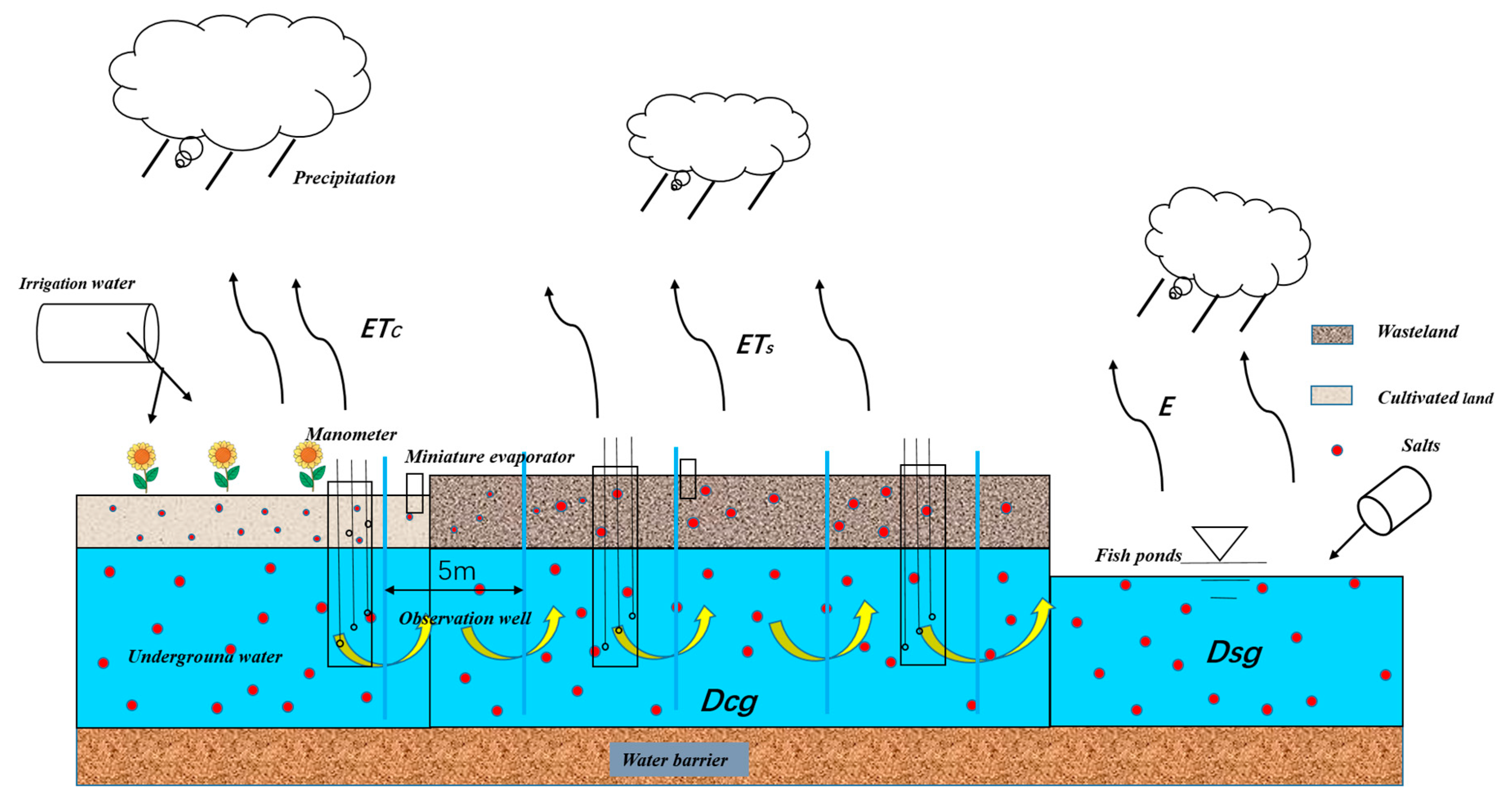
2.2. Test Layout and Data Acquisition

2.2.1. Groundwater Observation

Eight groundwater observation wells were installed in the study area, all with a depth of 5 m. Among them, two were in cultivated land, four in wasteland, and two at the boundary of fish ponds. The elevation of the cultivated land was 1022.06 m, and the elevation of the wasteland was 1022.46 m. The spring irrigation in the study area took place on 16 May 2022, with a water volume of about 150 mm, and the fall watering took place on 30 September 2022, with a water volume of about 200 mm. During the fall watering period, farmers recharged the fish ponds with water. The average mineralization of irrigation water was 1.05 g/L. Groundwater depth and conductivity were measured every 7 days, with additional measurements before and after rainfall and irrigation.

2.2.2. Soil Monitoring

There were 22 soil observation points, and the selected test area was divided into several 30 × 30 grids, with sampling in the center of the grid and encrypted sampling next to the groundwater observation wells. The sampling depth of the soil was 0–100 cm, and the soil was sampled in six layers: 0–10 cm, 10–20 cm, 20–40 cm, 40–60 cm, 60–80 cm, and 80–100 cm. A laser particle size analyzer was used to determine the particle size grading of the soil at the boundary of the cultivated wasteland and fish ponds, and the physical properties of the soil at the boundary of the cultivated wasteland and fish ponds are shown in

Table 1. Soil physical properties of typical sample points in the study area.

Land Type	Soil Depth (cm)	Soil Physical Properties				VG Parameter
		Clay (%)	Silt (%)	Sand (%)	Bulk Density (g.cm−3)	θr	θs	α	n	Ks	l
Cultivated land	0–10	5.48	67.54	26.98	1.63	0.036	0.3291	0.0105	1.5013	20.31	0.5
	10–20	5.67	65.5	28.83	1.61	0.0359	0.3299	0.0103	1.5048	21.22	0.5
	20–40	5.87	65.6	28.53	1.59	0.0369	0.3342	0.0096	1.5217	22.65	0.5
	40–60	4.81	72.64	22.55	1.57	0.0391	0.3487	0.0085	1.5636	27.7	0.5
	60–80	7.59	79.58	12.83	1.57	0.0482	0.3766	0.0072	1.5978	21.5	0.5
	80–100	4.70	64.4	30.9	1.55	0.0353	0.3362	0.0097	1.5279	28.74	0.5
Wasteland	0–10	5.54	63.31	31.15	1.58	0.0355	0.3317	0.0102	1.51	23.6	0.5
	10–20	7.64	68.36	24.00	1.57	0.0421	0.3484	0.0078	1.5688	21.18	0.5
	20–40	8.60	71.08	20.32	1.56	0.0458	0.3595	0.007	1.5939	20.51	0.5
	40–60	9.63	77.9	12.47	1.55	0.0521	0.3832	0.0065	1.6144	19.83	0.5
	60–80	6.94	79.89	13.17	1.53	0.0485	0.3835	0.0068	1.6164	26.63	0.5
	80–100	5.35	85.79	8.86	1.51	0.0495	0.4005	0.0071	1.6195	30.36	0.5
Fish pond boundary	0–10	5.21	68.09	26.7	1.54	0.0383	0.3458	0.0083	1.5632	29.82	0.5
	10–20	6.16	66.54	27.3	1.53	0.0395	0.3477	0.0079	1.5708	28.27	0.5
	20–40	9.65	75.44	14.91	1.53	0.0514	0.3805	0.0063	1.6245	21.65	0.5
	40–60	6.68	76.61	16.71	1.52	0.0464	0.375	0.0068	1.6177	28.71	0.5
	60–80	7.03	73.36	19.61	1.51	0.0455	0.3695	0.0066	1.619	28.96	0.5
	80–100	3.40	74.28	22.32	1.49	0.0396	0.3631	0.0075	1.605	42.55	0.5

. The water content of the soil was measured by the drying method, and the soil leachate with a water-to-soil ratio of 1:5 was measured by a conductivity meter (DDS-307A, Shanghai Youke Instrument Co., Ltd., Shanghai, China).

2.2.3. Water Sample Collection

Irrigation water, groundwater samples, and fish pond water samples were collected once every 7 days. Three replicates were collected each time, and their conductivity was measured by a conductivity meter.

2.2.4. Soil Water Potential

Two groups of field negative pressure meters were installed at the boundaries of arable land, wasteland, and fish ponds at depths of 60, 80, and 100 cm, respectively, the soil–water potentials at the boundaries of arable land, wasteland, and fish ponds were measured, and the averages of the two groups were taken, respectively.

2.3. Research Methods

2.3.1. Sample Processing

The conversion of soil electrical conductivity to soil total salt content calculation formula is as follows [18]:

$$C=3.7657E{C}_{1:5}-0.2405$$

(1)

where C represents the soil total salt content (g/kg), and EC_1:5 denotes the soil water mass ratio of 1:5 soil extract conductivity (ds/m).

The formula of soil salt content is as follows [19]:

$$S=100C{\rho }_{s}l$$

(2)

where S represents the soil salt content (kg/hm²), ρ_s denotes the volume weight of soil (g/cm³), and l indicates the soil depth (cm).

Using the empirical formula developed by the laboratory, the groundwater conductivity is converted into groundwater salinity. The formula is as follows:

$$T_{DS}=0.69EC$$

(3)

2.3.2. Calculation of Groundwater Recharge

In this paper, the positioning flux method is used to calculate groundwater recharge. The positioning flux method is to install a negative pressure gauge at a specific position Z₁ and Z₂. By monitoring the change in soil water potential gradient, the flux at this point is calculated by West’s law [20] and is calculated via the following formula:

$$Q(z_{1-2})=-K(\overline{h})(\frac{h_2-h_1}{\Delta Z}+1)$$

(4)

of which:

$$\overline{h}=\frac{h_1+h_2}{2}$$

(5)

$$K(h)=\alpha mn\alpha {\theta }_s{(\alpha h)}^{n-1}{\left[1+{(\alpha h)}^n\right]}^{-m-1}.\exp {(b\theta s\left[1+{(\alpha h)}^n\right])}^{-m}$$

(6)

where h₁ and h₂ represent the negative pressure at Z₁ and Z₂ of the section measured (hPa), ∆Z denotes the difference between Z₂ and Z₁ (cm), Q(Z₁₋₂) indicates the soil water flow per unit area in the t₁~t₂ period (mm), K(h) is the unsaturated hydraulic conductivity (cm/min), θs is the saturated soil moisture content (cm³/cm³), α is the reciprocal of the soil air intake value (cm⁻¹), h is the soil suction (hPa), and m and b form the fitting empirical parameters.

The flow rate of any section can also be obtained from Q(Z₁₋₂):

$$Q(z)=Q(z_{1-2})+{\displaystyle \underset{z}{\overset{z_{1-2}}{\int }}Q(z,t_2)dz-{\displaystyle \underset{z}{\overset{z_{1-2}}{\int }}Q(z,t_1)dz}}$$

(7)

2.3.3. Calculation of Soil Salinity for Groundwater Recharge

Groundwater recharge soil salt formula:

$$S_b=10005\frac{N_d{\displaystyle \sum _{i=1}^2\overline{Q_i}(z)\overline{TDS}}}{1000\phi }$$

(8)

where S_b is the groundwater recharge soil salt content (kg/hm²), N_d is the computing time (days), $\overline{Q_{\mathrm{i}}}(z)$ is the average groundwater recharge in the soil layer (mm/d), $\overline{TDS}$ is the average salinity of groundwater (g/L), and φ is the soil porosity value as 0.36.

2.3.4. Calculation of Osmotic Salts

Based on the theory of salt balance, the formula for calculating the horizontal infiltration salt amount of cultivated land is as follows:

$$S_l=S_i-S_{i-1}-S_{ib}-S_{is}$$

(9)

where S_i is the salt storage of wasteland in the i period (kg/hm²), S_i−1 is the salt storage of wasteland in the i − 1 period (kg/hm²), S_ib is the salt content of groundwater recharge to wasteland in period i − 1~i (kg/hm²), and S_is is the accumulated salt content of wasteland (0–60 cm) in period i~1 − i (kg/hm²).

2.3.5. Calculation of Soil Salt Accumulation Rate

The soil salt accumulation rate is the increased rate of soil salt content in a certain period of 0–100 cm soil profile compared with the previous period. The calculation formula is as follows:

$$t=\frac{W_i-W_{i-1}}{W_i}\times 100\%$$

(10)

where t is the soil salinity (%), W_i is the soil salt content in period i (kg/hm²), and W_i−1 is the soil salt content in period i − 1 (kg/hm²).

2.3.6. Soil Desalinization Rate Calculation

The soil desalinization rate is 0~100 cm average soil profile in a period of time after irrigation compared with the before-irrigation soil salt content reduction rate, and the calculation formula is as follows:

$$\omega =\frac{s_0-s_t}{s_0}\times 100\%$$

(11)

where ω is the soil desalinization rate (%), S_t is the soil salt content in a certain period after irrigation (kg/hm²), and S₀ is the soil salt content before irrigation (kg/hm²).

2.3.7. Estimation of Groundwater Migration

The formula for calculating the hydraulic gradient of the cross section of cultivated wasteland is as follows:

$$J_i{}_1=\frac{h_{ci}-h_{wi}}{L}$$

(12)

where J_i1 is the hydraulic gradient between cultivated land and wasteland, i is the ith stress period, h_ci is the groundwater level of the cultivated land observation point (m), h_wi is the groundwater level of the salt wasteland observation point (m), and L is the distance between the cultivated–wasteland observation points of each water cross section (m).

The formula for calculating the hydraulic gradient of the water section of the fish pond in the wasteland is as follows:

$$J_i{}_2=\frac{h_{wi}-h_{fi}}{L}$$

(13)

where J_i2 is the hydraulic gradient between wasteland and fish pond, i is the ith stress period, h_wi is the groundwater level of the wasteland observation point (m), h_fi is the groundwater level of the fish pond observation point (m), and L is the distance between the wasteland and the fish pond observation point (m).

According to Dupuit’s basic differential equation, the unit width flow formula of each cross section of cultivated wasteland can be obtained as follows:

$$q_i{}_1=KD{J}_{i1}=KD\frac{h_{ci}-h_{wi}}{L}$$

(14)

where q_i1 is the unit width flow of groundwater between cultivated land and wasteland every day (m²/d), and K is the permeability coefficient in the horizontal direction. According to the existing research results [21], the value is 6.26 m/d, D is the thickness of the phreatic aquifer in the study area. According to the relevant literature [22], the value is 22.5 m.

The unit width flow formula of each cross section of wasteland–fish pond is as follows:

$$q_i{}_2=KD{J}_{i2}=KD\frac{h_{wi}-h_{fi}}{L}$$

(15)

where q_i2 is the unit width flow of groundwater between fish ponds in wasteland every day (m²/d), K is the permeability coefficient in the horizontal direction, with a value of 6.26 (m/d), and D is the thickness of the phreatic aquifer in the study area. According to the relevant literature, the value is 22.5 m.

The formula for calculating the amount of water transferred from cultivated land groundwater to salt wasteland is as follows:

$$Q_{c-w}={\displaystyle \sum _{i=1}^{30}{q}_i{}_1\times B}$$

(16)

where Q_c−w is the amount of water transferred from cultivated land groundwater to wasteland during the 30 stress periods in 2022 (m³), q_i1 is the average daily unit width flow of groundwater at the cultivated–wasteland boundary (m²/d), B is the total length of the cultivated–wasteland boundary (m). (Through the earth measurement of Bigemap GIS 2.9.2 software, we can see that the total length of the boundary between cultivated land and wasteland is 130.8 m).

The formula for calculating the amount of water transferred from wasteland groundwater to fish ponds is as follows:

$$Q_{w-f}={\displaystyle \sum _{i=1}^{30}{q}_{i2}\times B}$$

(17)

where Q_w−f is the amount of water transferred from wasteland to fishpond during 30 stress periods in 2022, and the negative value represents the amount of water transferred from fishpond to wasteland (m³), q_i2 is the average daily unit width flow of groundwater in wasteland–fish pond (m²/d), B is the total length of the wasteland–pond boundary (m). (The total length of the boundary between the wasteland and the fishpond is 95.7 m, as measured by Bigemap GIS software).

3. Results

3.1. Statistical Characteristics of Soil Salinity

Typical statistical analyses of the experimental observations in the study area in 2022 were carried out using SPSS 27 software, and the results are shown in

Table 2. Statistical analysis results of soil salt content g/kg.

Land Type	Soil Depth (cm)	Min	Max	Mean Vale	Standard Deviation	Coefficient of Variation	Bias Angle	Kurtosis
Cultivated land	0–10	1.68	3.07	2.31	0.50	0.22	0.64	1.52
	10–20	1.57	2.84	2.11	0.49	0.23	0.69	0.35
	20–40	1.27	2.23	1.87	0.40	0.21	−0.96	−0.55
	40–60	1.11	2.15	1.64	0.49	0.30	−0.40	−2.96
	60–80	0.84	1.85	1.42	0.49	0.35	−0.59	−3.17
	80–100	0.78	1.54	1.20	0.35	0.29	−0.55	−2.95
Wasteland	0–10	14.61	21.72	19.57	2.898	0.15	−1.779	3.381
	10–20	5.20	9.97	8.19	1.859	0.23	−1.270	1.626
	20–40	4.44	8.47	6.87	1.775	0.26	−0.745	−2.038
	40–60	4.11	8.13	6.46	1.900	0.29	−0.572	−2.902
	60–80	3.78	6.33	5.28	1.288	0.24	−0.598	−3.238
	80–100	3.20	5.75	4.58	1.128	0.25	−0.434	−2.656
Fish pond boundary	0–10	10.08	11.46	10.92	0.580	0.05	−0.689	−0.650
	10–20	4.14	8.26	6.21	1.638	0.26	−0.139	−1.310
	20–40	3.38	5.00	4.23	0.777	0.18	−0.444	−3.080
	40–60	2.48	4.44	3.75	0.885	0.24	−0.899	−1.408
	60–80	2.83	5.41	3.88	1.046	0.27	0.685	−0.475
	80–100	2.46	4.35	3.64	0.854	0.23	−0.796	−2.019

. The coefficient of variation (COV) reflects the degree of dispersion of the experimental observations, and in soil science, the degree of variability in soil properties is categorized according to the value of the coefficient of variation (CV): CVs of 0–0.15 are considered to be weak, 0.16–0.35 are considered to be moderate, and greater than 0.36 are considered to be strong [23].

By analyzing the statistical results of the conductivity of 1:5 soil leachate (Table 2), it can be seen that the coefficients of variation (CV) of salinity of different land types at different soil depths in the study area were weakly variable, except for the coefficient of variation (CV) of the 0–10 cm soil layer on the border of the fish pond, which was weakly variable from 0 to 0.15, and the rest of the coefficients of variation (CV) of the soil layers were moderately variable from 0.16 to 0.35. The average salinity of soil of different land types showed a decreasing trend with the increase in soil depth, and the phenomenon of salinity surface aggregation was obvious. The salinity of 0–10 cm soil of wasteland was 8.47 times higher than that of 0–10 cm soil of arable land, and 1.74 times higher than that of 0–10 cm soil of fish pond boundary.

3.2. Salt Apparent Analysis

The results of soil salinity calculation are shown in Figure 3, calculated at the beginning of the spring irrigation period to before fall watering (1 May to 23 September). The crop planted in the arable land was sunflower; sowing started on 13 June and harvesting was carried out on 21 September, and the arable land was not irrigated during the reproductive period of the crop. In the 1 m soil body of arable land, during the spring irrigation period (1 May to 15 June), the soil desalinization was 4.56 t/hm², with a soil desalinization rate of 13%, and the soil salinity before the fall watering (23 September), the average value of the arable land salinity during the more fertile period (15 June to 22 August), was 22.64 t/hm², and the soil salinity accumulation was 7.54 t/hm², with a salinity accumulation rate of 25%.

The soil salt accumulation in the 1 m soil body of wasteland during the spring irrigation period (1 May to 15 June) was 6.99 t/hm², and the salt accumulation rate was 5.23%. Soil salinity before fall watering was 103.64 t/hm² compared to the average value of salinity during the crop fertility period (15 June to 22 August) in the wasteland, with a salt accumulation of 66.57 t/hm² and a salt accumulation rate of 39%.

During the spring irrigation period (1 May to 15 June), soil salt accumulation in the 1 m soil bordering the fish ponds was 3.63 t/hm², with a salt accumulation rate of 4%. Compared with the average salt value of 67.27 t/hm² during the crop fertility period (15 June to 22 August), the soil salt accumulation before fall irrigation was 17.92 t/hm², with a salt accumulation rate of 21%.

In summary, after one fertility period, the 1 m soil body of arable land failed to discharge the salts from the soil through spring irrigation drenching; because of the high temperature and strong evaporation in summer in the experimental area, the soil accumulated 25% of salts. Within the 1 m soil body of wasteland, salt accumulation was maintained throughout the reproductive period. The salt accumulation rate reached 44%; the 1 m soil body within the boundary of the fish pond also remained in a salt accumulation state throughout the reproductive period, but the salt accumulation rate was 25%, which was 0.57 times higher than that of the salt accumulation rate of the soil in the wasteland.

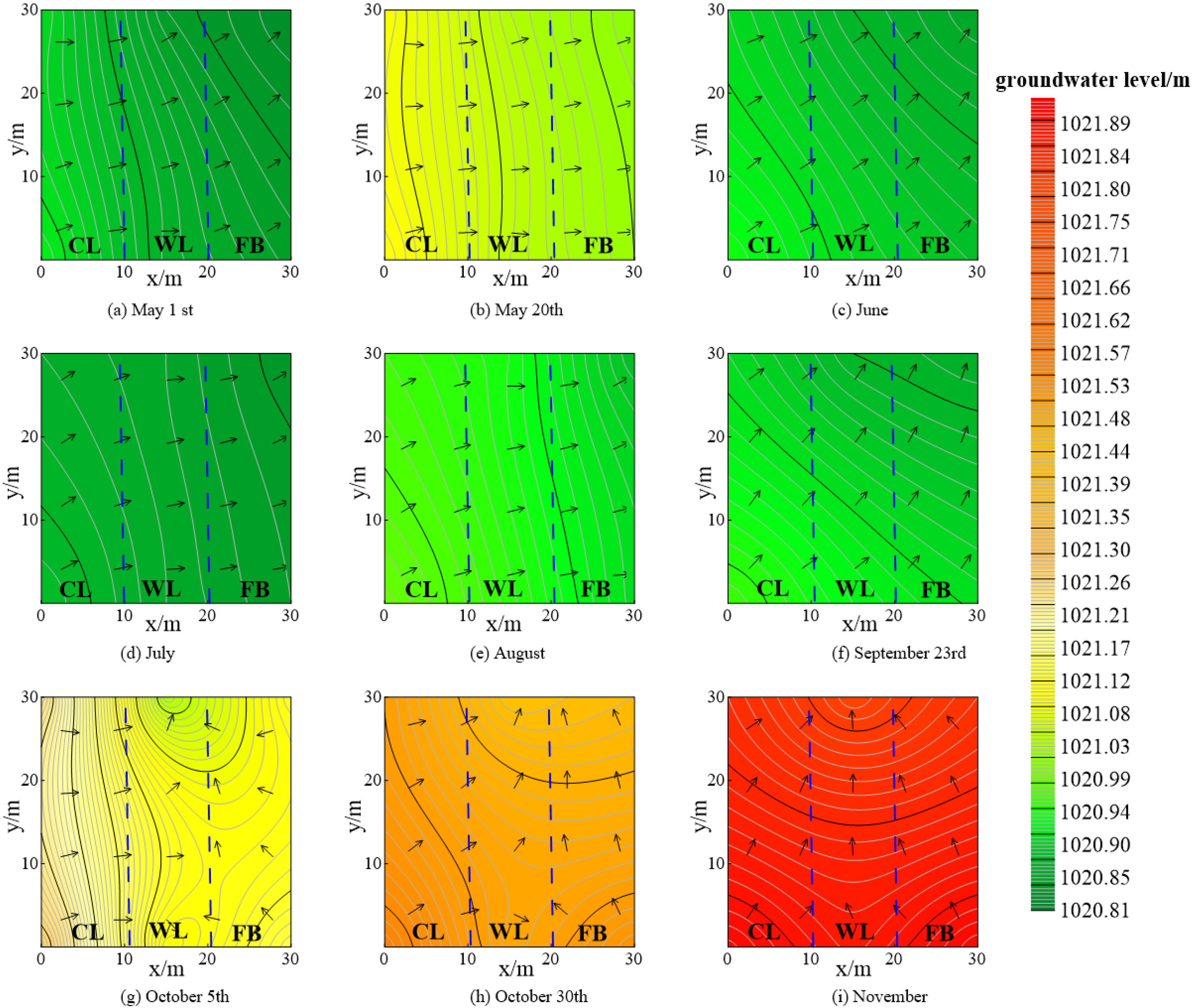
3.3. Groundwater Migration and Transformation in the Boundary of Cultivated Land–Wasteland–Fish Pond

In order to explore the water–salt conversion law between arable land–wasteland–fish ponds in different periods, based on the Grid Vector map of the surfer software, the change in groundwater level and the direction of groundwater transport were plotted as shown in Figure 4 (CL—cultivated land; WL—wasteland; FB—fish pond boundary). Groundwater level changes in the study area can be divided into 3 stages. There were 2 irrigation events throughout the year, and the irrigation time was May 16 and September 30, before and after these 2 nodes were encrypted to draw the groundwater level contour maps to respond to the changes in groundwater level. Groundwater level analysis was conducted every 1 month at other times.

(1) Spring irrigation stage (Figure 4a,b represent the water level changes before and after irrigation, respectively): the groundwater level of the cultivated land rose rapidly after irrigation, forming a water level difference with the unirrigated wasteland, and the migration of groundwater from the cultivated land to the wasteland groundwater became more obvious. The direction of groundwater migration was cropland–wasteland–fish pond.

(2) Fertility stage (Figure 4c–f): with the gradual increase in temperature, diving evaporation is strong, and the groundwater level of cultivated wasteland decreases month by month. Sunflower is planted in this study area, and there is no irrigation during the fertility stage and less rainfall, so the change in the groundwater level during the fertility stage is small. The water level in the wasteland and fish ponds tends to be the same, except for the cultivated land, which is slightly fluctuated by the influence of irrigation in the surrounding land (tomato and corn farmland). Fish ponds have greater evaporation of water surface in this stage and less water recharge in this period, so the water level also decreased; however, the direction of groundwater migration is still cultivated land–wasteland–fish ponds.

(3) Autumn watering stage (Figure 4f–i, where f represents the change in water level before irrigation; g represents the change in water level at the early stage of irrigation; Figure 4h,i represent the change in water level at the end of irrigation): Because of the large amount of water used for autumn watering and the recharge of water to fish ponds by farmers at this stage, the change in groundwater level is more drastic, and the water level reaches the lowest point of the whole year before irrigation (Figure 4f), then rises rapidly due to the irrigation, as shown in Figure 4g for the early stage of irrigation, which is the first stage of irrigation. Under the influence of fall watering, the groundwater of cultivated land is recharged by irrigation water, the groundwater level rises significantly, the unirrigated wasteland forms an obvious water level difference, and the migration of groundwater to the wasteland is more significant; at the same time, farmers recharge the water to the fish ponds, which leads to a rapid rise in the water level of the fish ponds, the adjacent wasteland forms a water level difference, and the water of the fish ponds migrates to the wasteland; Figure 4h,i are the end of the irrigation period, and it can be seen that, with the passage of time, the groundwater level changes are more obvious, the groundwater level of cultivated land and the groundwater level of fish pond boundary continue to rise. At the end of irrigation, the direction of groundwater migration is changed, and the groundwater levels of cultivated land and fish ponds migrate to the groundwater of wasteland at the same time.

According to Equations (12)–(17), the amount of water migrating from groundwater in cropland to wasteland in the simulation period of 2022 is 2700 m³, the amount of water migrating from groundwater in wasteland to fish pond is 630 m³, and the amount of water migrating from fish pond to groundwater in wasteland during fall watering is 440 m³.

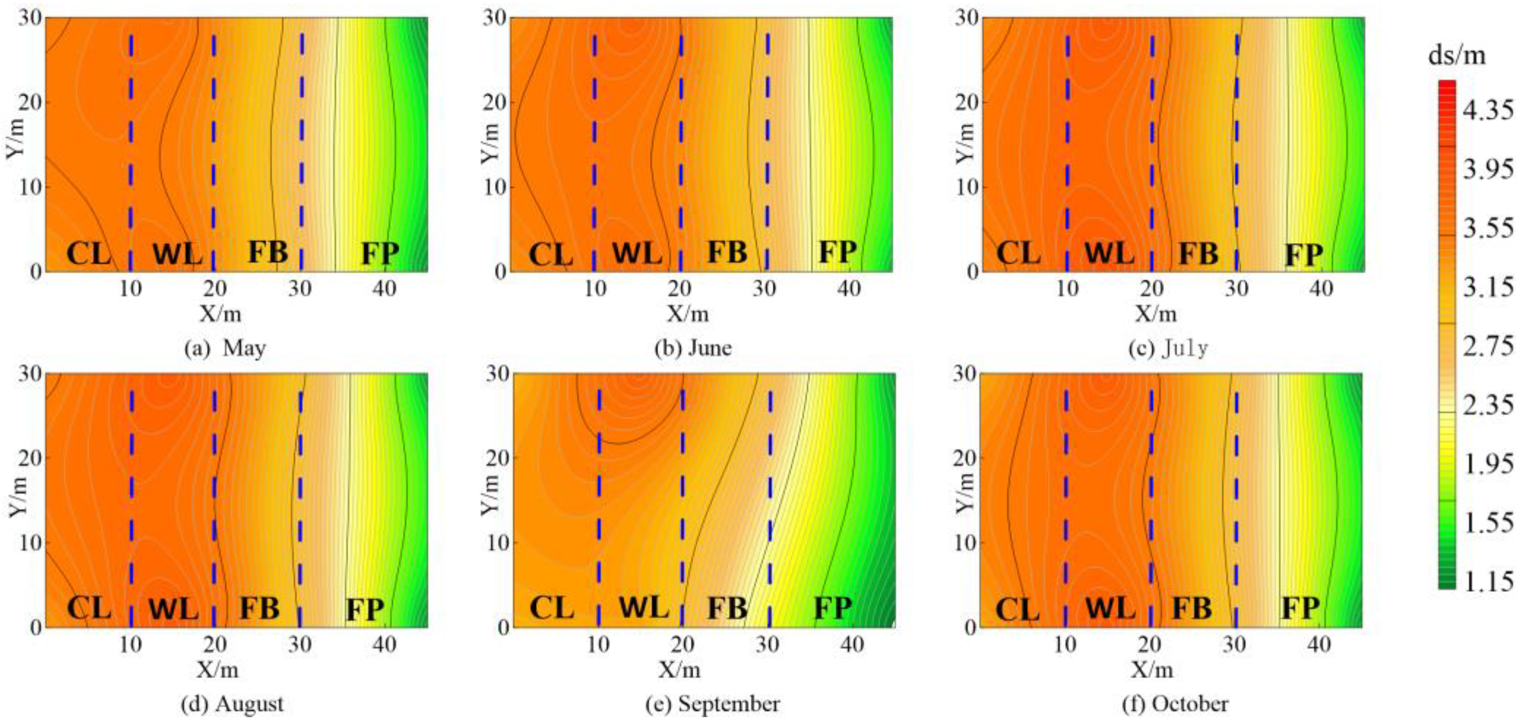
3.4. The Variation Law of Groundwater EC in the Boundary of Cultivated Land–Wasteland–Fish Pond

Groundwater mineralization indicates all anions and cations in the water. Groundwater mineralization is an important indicator of changes in groundwater quality under the influence of human activities [24]. Changes in the concentration of chemical components, especially macronutrients, in groundwater will cause changes in mineralization. Therefore, the mineralization degree can well respond to the distribution characteristics and change trends of material components in groundwater in general. In this paper, the measured EC data of groundwater in cropland, wasteland groundwater, and fish pond water in different periods in 2022 were utilized to map the temporal and spatial changes in groundwater EC based on the Universal Kriging interpolation method (Figure 5) (CL–cultivated land; WL–wasteland; FB–fish pond boundary; FP–fish pond). As shown in Figure 5: (1) The mean value of groundwater EC in the study area was 3.27 ds/m for cultivated land; the mean value of groundwater EC in wasteland was 3.71 ds/m, which was close to cultivated land, and 1.13 times higher than cultivated land. The mean value of conductivity of the fish pond is 1.22 ds/m, which is 0.37 times that of groundwater of cultivated land; the mean value of conductivity of groundwater at the boundary of the fish pond is 2.73 ds/m, which is 0.83 times that of groundwater of cultivated land and 0.73 times that of groundwater of wasteland. The reason for this is as follows: under the action of irrigation water, the salts in the arable land that were washed into the groundwater flowed to the wasteland along with the groundwater of the arable land, and at the same time, the evaporation of the soil of the wasteland was intense, which led to the wasteland being the most serious salinization area. And the fish pond is recharged with Yellow River water, which dilutes the groundwater at the boundary of the fish pond when the water from the fish pond flows to the groundwater of the wasteland. (2) The reason for the monthly and seasonal changes in groundwater EC value within the year is that the changes in groundwater EC value are directly affected by groundwater recharge and discharge. Infiltration water incorporates a large amount of salts in the soil into the groundwater due to the influence of salt suppression by spring irrigation and autumn watering, resulting in the groundwater mineralization remaining at a high level during the irrigation period.

3.5. Estimation of Water and Salt Migration in Wasteland

Wasteland is in the middle of cultivated land and fish ponds, soil water salinity is greatly affected by cultivated land and fish ponds, and when cultivated land is irrigated or fish ponds are recharged, the groundwater level will be raised accordingly, resulting in a difference in the water level and the neighboring cultivated land to produce horizontal lateral exchange inf groundwater. During the crop reproductive period, the sources of soil moisture recharge in the wasteland are capillary recharge of groundwater in the wasteland and rainfall recharge. The rainfall mineralization in the study area is very small and negligible, so the sources of salinity in the wasteland are the horizontal hydrodynamic diffusive recharge of salts from cultivated soils and groundwater capillary recharge. The mineralization of groundwater in wasteland has a significant influence from the groundwater from cultivated land and groundwater from fish ponds. Wasteland groundwater depletion is mainly the surface evapotranspiration evaporation effect.

For salt migration estimation of 1 m soil body from the beginning of sunflower sowing to before autumn watering (15 June–23 September, 101 days), it can be seen from Figure 3 that the salt accumulation of wasteland was 36.55 t/hm², and the salt accumulation of 0~60 cm soil layer of wasteland was 31.04 t/hm², which accounted for 85% of the salt accumulation of wasteland. From Equations (4)–(7), the groundwater recharge of each soil layer in the wasteland is shown in Figure 6, and the average groundwater recharge of 60~80 cm and 80~100 cm soil layer is 0.54 and 0.47 mm/d, respectively. From Equation (3), the average groundwater mineralization in the wasteland is 2.62 g/L. From Equation (8), the groundwater recharge of soil salt in the wasteland is 3.71 t/hm², accounting for 10% of the salt accumulation, 10% of the salt volume. From Equation (9), it can be seen that the horizontal infiltration of cultivated land to the wasteland salt amount is 1.79 t/hm², accounting for 5% of the accumulation of salt.

3.6. Effect of Fish Pond on Soil Salinity

Existing studies have shown the significant effect of fish ponds on saline land improvement [25]. According to the experimental monitoring data, the mean value of soil salinity in the 0–10 cm soil layer of the wasteland was 19.57 g/kg, the mean value of soil salinity in the 0–10 cm soil layer at the boundary of the fish pond was 10.92 g/kg, and the salinity of the soil at the boundary of the fish pond was reduced by a factor of 0.56 compared with that in the wasteland; the mean value of the groundwater level in the wasteland was 1020.9 m, the mean value of the groundwater level at the boundary of the fish pond was 1020.42 m, and the groundwater level at the boundary of the fish pond was 0.48 m lower than that of the wasteland; the amount of water migrating from the wasteland groundwater to the fish pond during the simulation period was 630 m³, and the amount of water migrating from the fish pond to the wasteland groundwater during the fall watering period was 440 m³. The mean value of the groundwater EC of the wasteland groundwater was 3.71 ds/m, the mean value of the groundwater EC at the boundary of the fish pond was 2.73 ds/m, and the EC of groundwater at the boundary of the fish pond was 0.99 ds/m lower than that of groundwater in the wasteland.

In summary, controlling the water level in fish ponds during the crop fertility stage can reduce soil salinization by lowering the wasteland groundwater level to inhibit surface evaporation. After replenishing water in the fall watering stage, soil salinity can be reduced by diluting the EC value of wasteland groundwater. Reasonable control of the water level in fish ponds has a positive effect on saline land improvement without bringing a greater risk of soil salinization. According to the results of a survey of farmers, the average income from saline fish ponds is $3000/hm², the construction of fish ponds in wasteland effectively utilizes land resources and realizes the multifunctional use of land. At the same time, fish ponds can improve the surrounding environment, improve the ecological benefits of the land, and promote the development of the local economy. The role of fish ponds in the improvement of saline land is multifaceted and can have a positive impact on the economy, ecology, and society.

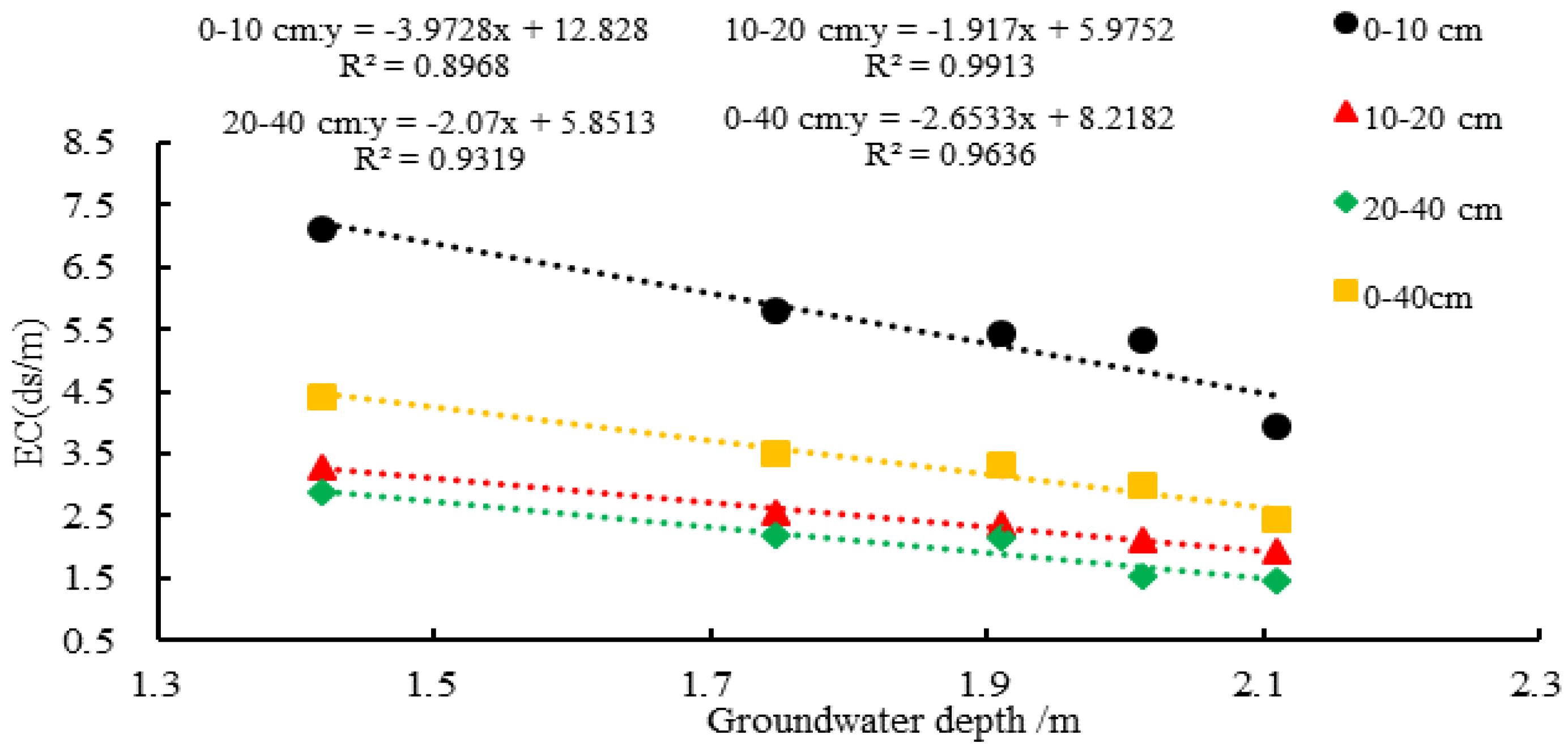
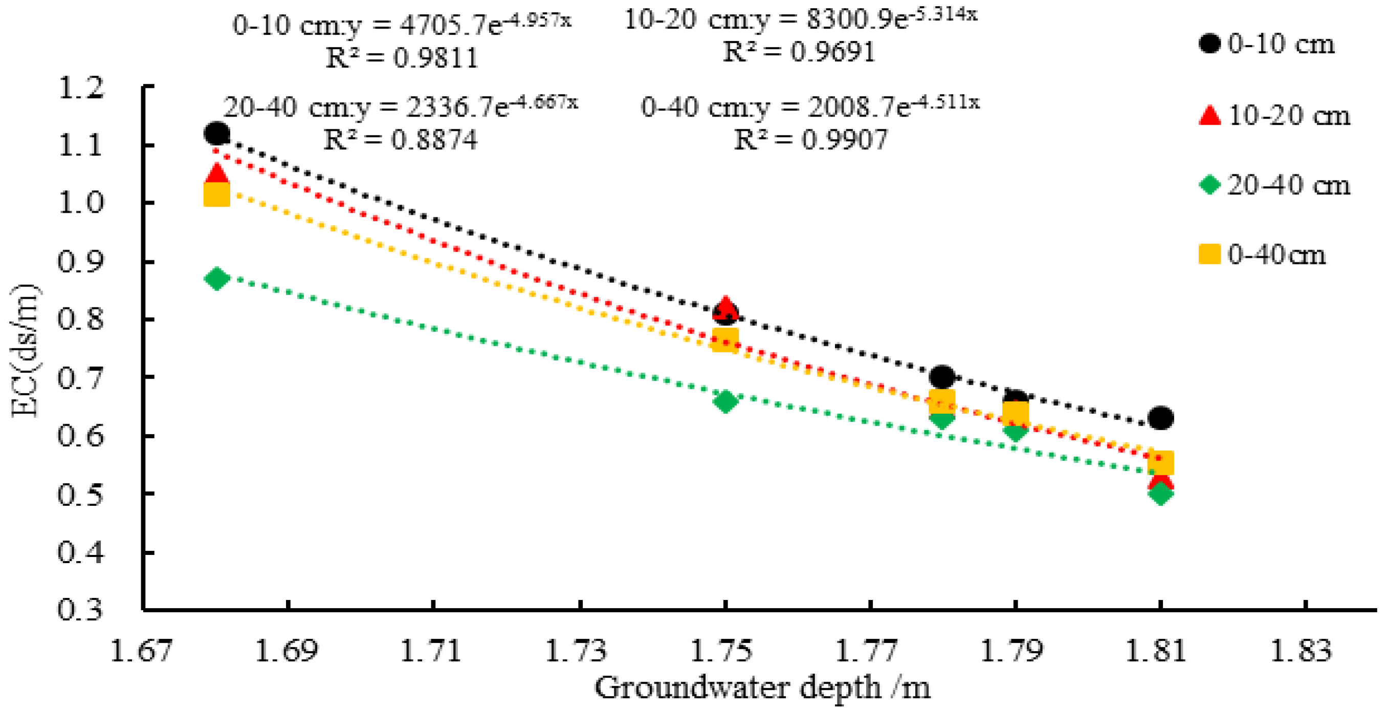
3.7. Effect of Groundwater Depth on Soil Salinity

Research shows that the soil salt content is most affected by the water table and the mineralization of groundwater, and the depth of groundwater is a decisive factor in the occurrence of soil salinization. In the river-loop irrigation area, the depth of groundwater is shallow, and the groundwater contains more soluble salts, which are brought to the surface of the soil by evaporation and lead to the accumulation of salt in the soil, so controlling the depth of groundwater is crucial for the improvement of soil salinization in the river-loop irrigation area.

The monthly average values of 8 groundwater observation wells in the study area and the EC1:5 average values of 22 soil (0–10 cm, 10–20 cm, 20–40 cm, 0–40 soil layer average) layers per month were selected to plot the relationship between soil salinity and groundwater burial depth in wasteland, and the relationship between soil salinity and groundwater burial depth in cultivated land, respectively (Figure 7 and Figure 8).

As shown in Figure 7, the soil salinity and groundwater burial depth of wasteland satisfy the linear relationship, R² > 0.8968, the soil salinity decreases with the increase in groundwater burial depth, and the salinity of the 0–10 cm soil layer of wasteland has a larger trend of change with the depth of groundwater; as shown in Figure 8 the soil salinity of arable land satisfies the exponential relationship with the depth of groundwater, R² > 0.8874, and when groundwater depth is in the range of 0~1.75 m, the soil conductivity EC1:5 varies greatly with the depth of groundwater burial, and soil EC_1:5 conductivity decreases with the increase in soil depth; when the depth of groundwater burial is greater than 1.75 m, the change in soil conductivity with the increase in soil depth is not significant, and the soil conductivity is below 0.66 ms/cm, which has less impact on the growth of crops and basically does not cause crop yield reduction. Existing studies have shown [26,27] that a shallow groundwater burial depth of 1.5~2.5 m is favorable for crop growth, but from the perspective of salinization control, the appropriate depth of groundwater burial should be controlled at about 2.0 m. Therefore, exploring methods to control the critical depth of groundwater burial depth to ensure that it does not affect crop growth and does not exacerbate soil salinization is an urgent problem that needs to be solved. And this study shows that when the water level of fish ponds is lower than the groundwater level of wasteland, it can reduce the groundwater level of wasteland, so we need to control the water level of fish ponds so that it is lower than the groundwater level of wasteland during the evaporation-sensitive period, so it is significant to explore the mechanism of water and salt transport in arable wasteland under the influence of fish ponds.

4. Discussion

The area of soil salinization in the Hetao Irrigation District of Inner Mongolia is about 330,000 hm², accounting for 63% of the total cultivated area. Soil salinization has become one of the prominent problems of land in today’s society [28,29,30], so many scholars have explored the effects of different factors on soil salinization with a view to providing a theoretical basis for improving and preventing soil salinization [31,32,33,34,35].

In order to explore the effect of saline–alkaline land on saline–alkaline land improvement, Fan et al. [36] analyzed the saline–alkaline bare soil, the silt of fish ponds in 3,5,8 a of fish ponds, and the soil of rice planting after 5 a of fish ponds, and concluded that the effect of saline–alkaline land improvement was different in different years of fish ponds, and that rice planting after 5 a of fish ponds was the most effective way of improving the saline–alkaline land. Mandal et al. [37] evaluated different land shaping patterns and showed that farm ponds, rice-cum-fish systems, etc., can increase cropping intensity and net farm income, reduce salinity in the summer, reduce flooding in the rainy season, and improve soil quality (Batukaev et al. [38]). Calcium carbonate equilibrium algorithms, mathematical models, and original software were developed for calculating the true equilibrium form of calcium carbonate and determining the nature of the equilibrium of calcium carbonate in solution. Representation of the carbonate system in aqueous solutions of soils and air inclusion zones helps to explain the evolution of saline soils, air inclusion zones, and saturated zones, as well as landscapes, and also helps to improve soil maintenance, plant nutrition, and irrigation. Guan et al. [23] showed that when the soil conductivity is less than 0.8 ms/cm, it has less impact on corn and wheat, etc., and basically does not cause crop yield reduction. Narjary et al. [39] used the Hydrus-1D model to simulate the effects of shallow saline groundwater burial depth and evaporative flux on soil salt transport, and the results showed that summer is the most important period for controlling soil salinity. Khasanov et al. [40], by combining traditional research methods and cross-validated GIS methods, analyzed the spatial variations of groundwater level, groundwater mineralization, and soil salinity induced by climatic factors from 2000 to 2019, and they concluded that groundwater mineralization and groundwater level are the main factors influencing soil salinization. Malik et al. [41] indicated that the depth of groundwater burial affects soil moisture, soil temperature, and surface temperature, and they indicated that soil moisture is strongly negatively correlated with the water table (Li et al. [42]) In order to study the temporal and spatial distribution law of soil salinization, the temporal and spatial change law of groundwater depth in the saline and alkaline land of the Yellow River was analyzed. The results of the study showed that the changes in groundwater depth were divided into the fall watering stage, freeze–thaw stage, and crop fertility stage, and that fall watering and irrigation caused antisalinity in the surface layer of the soil in spring.

In this study, the difference between cultivated land and wasteland under the influence of artificial fish ponds was selected. Fish ponds can not only improve the soil structure of saline and alkaline land but also play a positive role in the ecological environment. Fish ponds of an appropriate scale can improve the ecological environment of rivers, lakes, and other waters. By breeding fish, the circulation and oxidation of the water body can be strengthened to promote the decomposition of the substrate and improve water quality, which will help to restore the ecological environment. Moreover, the fish ponds have a low topography, and the water in the fish ponds has a low mineralization, which is a more special salt wasteland land type in the river-loop irrigation area.

5. Conclusions

(1) Observational data showed that soil salinity and groundwater mineralization varied considerably among the locations of the observation wells. The groundwater observation wells at the boundary of the fish ponds have a large depth of groundwater, small groundwater mineralization, and relatively small salinity compared to the wasteland. In the river-loop irrigation area, where salinization is serious, the fish ponds play a role in reducing soil salinization and, at the same time, increase the economic income of local farmers, which in turn promotes local economic development.

(2) In the cropland–wasteland–fish pond system, the spatial distribution of salts in the groundwater and fish pond was consistent. The soluble salts that were drenched into the groundwater during the spring irrigation period migrated to the fish pond along with the groundwater, and after the farmers replenished the fish pond during the autumn watering stage, the water in the fish pond flowed backward into the groundwater of the wasteland, which played a role in diluting the mineralization of the groundwater of the wasteland.

(3) There is an exponential relationship between groundwater depth and soil salinity. When the depth of groundwater is greater than 1.75 m, the change in soil salinity with depth of groundwater is small, so it can be controlled by controlling the water level of fish ponds to control the depth of groundwater in the range of 1.75 to 2.0 m.

(4) Fish ponds inhibit shallow water evaporation by lowering the groundwater level in the cultivated wasteland during the crop reproductive period, thus reducing soil salinity, and reduce soil salinity by diluting groundwater mineralization in the fall.

References

1. Pereira, L.S.; Goncalves, J.M.; Dong, B.; Mao, Z.; Fang, S.X. Assessing basin irrigation and scheduling strategies for saving irrigation water and controlling salinity in the upper Yellow River Basin, China. Agric. Water Manag. 2007, 93, 109–122. [Google Scholar] [CrossRef]
2. Ramos, T.B.; Liu, M.; Paredes, P.; Shi, H.; Feng, Z.; Lei, H.; Pereira, L.S. Salts dynamics in maize irrigation in the Hetao plateau using static water table lysimeters and HYDRUS-1D with focus on the autumn leaching irrigation. Agric. Water Manag. 2023, 283, 108306. [Google Scholar] [CrossRef]
3. Zhou, L. Influences of deficit irrigation on soil water content distribution and spring wheat growth in Hetao Irrigation District, Inner Mongolia of China. Water Supply 2020, 20, 3722–3729. [Google Scholar] [CrossRef]
4. Mousong, W.; Huang, J.; Xiao, T.; Jingwei, W. Water, salt and heat influences on carbon and nitrogen dynamics in seasonally frozen soils in Hetao Irrigation District, Inner Mongolia, China. Pedosphere 2019, 29, 632–641. [Google Scholar] [CrossRef]
5. Haj-Amor, Z.; Hashemi, H.; Bouri, S. Soil salinization and critical shallow groundwater depth under saline irrigation condition in a Saharan irrigated land. Arab. J. Geosci. 2017, 10, 301. [Google Scholar] [CrossRef]
6. Qureshi, A.S.; Ahmad, W.; Ahmad, A.F.A. Optimum groundwater table depth and irrigation schedules for controlling soil salinity in central Iraq. Irrig. Drain. 2013, 62, 414–424. [Google Scholar] [CrossRef]
7. Said, I.; Salman, S.A.; Elnazer, A.A. Salinization of groundwater during 20 years of agricultural irrigation, Luxor, Egypt. Environ. Geochem. Health 2022, 44, 3821–3835. [Google Scholar] [CrossRef]
8. Sarrazin, B.; Wezel, A.; Guerin, M.; Robin, J. Pesticide contamination of fish ponds in relation to crop area in a mixed farmland-pond landscape (Dombes area, France). Environ. Sci. Pollut. Res. 2022, 29, 66858–66873. [Google Scholar] [CrossRef]
9. Jia, Y.H.; Zheng, Y.H.; He, T.; Tang, H.Y. Effects of integrated rice-frog farming on soil bacterial community composition. Chil. J. Agric. Res. 2023, 83, 525–538. [Google Scholar] [CrossRef]
10. Ogburn, D.M.; White, I. Integrating livestock production with crops and saline fish ponds to reduce greenhouse gas emissions. J. Integr. Environ. Sci. 2011, 8, 39–52. [Google Scholar] [CrossRef]
11. Riley, W.D.; Potter, E.C.E.; Biggs, J.; Collins, A.L.; Jarvie, H.P.; Jones, J.I.; Kelly-Quinn, M.; Ormerod, S.J.; Sear, D.A.; Wilby, R.L.; et al. Small Water Bodies in Great Britain and Ireland: Ecosystem function, human-generated degradation, and options for restorative action. Sci. Total Environ. 2018, 645, 1598–1616. [Google Scholar] [CrossRef] [PubMed]
12. Zeng, J.; Liu, X.; Li, J.; Xia, Y. Dynamic analysis of water and salt in cropland—Saline alkali land—Sand dunes—Lake area based on SWAP model. J. Agric. Resour. Environ. 2018, 35, 540–549. [Google Scholar] [CrossRef]
13. Wang, G.S.; Xu, B.; Tang, P.C.; Shi, H.B.; Tian, D.L.; Zhang, C.; Ren, J.; Li, Z.K. Modeling and Evaluating Soil Salt and Water Transport in a Cultivated Land-Wasteland-Lake System of Hetao, Yellow River Basin’s Upper Reaches. Sustainability 2022, 14, 14410. [Google Scholar] [CrossRef]
14. Chughtai, M.I.; Mahmood, K. Semi-intensive Carp Culture in Saline Water-Logged Area: A Multi-Location Study in Shorkot (District Jhang), Pakistan. Pak. J. Zool. 2012, 44, 1065–1072. [Google Scholar]
15. Oron, G.; Appelbaum, S.; Guy, O. Reuse of brine from inland desalination plants with duckweed, fish and halophytes toward increased food production and improved environmental control. Desalination 2023, 549, 116317. [Google Scholar] [CrossRef]
16. Nguyen, H.L.; Tran, D.H. Saline Soils and Crop Production in Coastal Zones of Vietnam: Features, Strategies for Amelioration and Management. Pak. J. Bot. 2020, 52, 1327–1333. [Google Scholar] [CrossRef]
17. Mustafa, A.; Ratnawati, E.; Undu, M.C.; IOP. Characteristics and management of brackishwater pond soil in South Sulawesi Province, Indonesia. In Proceedings of the 3rd International Symposium on Marine and Fisheries (ISMF), South Sulawesi, Indonesia, 5–6 June 2020. [Google Scholar]
18. Zhao, Y.; Shi, H.; Miao, Q.; Yang, S.; Hu, Z.; Hou, C.; Yu, C.; Yan, Y. Analysis of Spatial and Temporal Variability and Coupling Relationship of Soil Water and Salt in Cultivated and Wasteland at Branch Canal Scale in the Hetao Irrigation District. Agronomy 2023, 13, 2367. [Google Scholar] [CrossRef]
19. Zhao, Y.; Li, Y.; Wang, J.; Pang, H.; Li, Y. Buried straw layer plus plastic mulching reduces soil salinity and increases sunflower yield in saline soils. Soil Tillage Res. 2016, 155, 363–370. [Google Scholar] [CrossRef]
20. Lei, Z. Soil Water Dynamics; Tsinghua University Press: Beijing, China, 1988. [Google Scholar]
21. Yang, W.; Mao, W.; Yang, Y.; Zhu, Y.; Yang, J. Optimizing Conjunctive Use of Groundwater and Cannel Water in Hetao Irrigation District Aided by MODFLOW. J. Irrig. Drain. 2021, 40, 93–101. [Google Scholar] [CrossRef]
22. Yuan, C. Monitoring Analysis and Numerical Simulation of Soil Water-Salt Dynamics under Irrigation Conditions in Arid Area of Northwest China. Ph.D. Thesis, Yangzhou University, Yangzhou, China, 2021. [Google Scholar]
23. Guan, X.; Wang, S.; Gao, Z. Spatio-temporal variability of soil salinity and its relationship with the depth to groundwater in salinizationirrigation district. ACTA Ecol. Sin. 2012, 32, 198–206. [Google Scholar] [CrossRef]
24. Barmakova, D.B.; Rodrigo-Ilarri, J.; Zavaley, V.A.; Rodrigo-Clavero, M.-E.; Capilla, J.E. Spatial analysis of the chemical regime of groundwater in the karatal irrigation Massif in South-Eastern Kazakhstan. Water 2022, 14, 285. [Google Scholar] [CrossRef]
25. Wu, Y.; Fan, F.; Ma, J.; Li, F.; Zhang, Q. Study on changes of fish pond water quality and soil physical and chemical properties during the improvement of saline alkali soil for fish culture in Embankments. Agric. Sci. J. Yanbian 2022, 44, 45–51. [Google Scholar]
26. Karimov, A.K.; Simunek, J.; Hanjra, M.A.; Avliyakulov, M.; Forkutsa, I. Effects of the shallow water table on water use of winter wheat and ecosystem health: Implications for unlocking the potential of groundwater in the Fergana Valley (Central Asia). Agric. Water Manag. 2014, 131, 57–69. [Google Scholar] [CrossRef]
27. Sharda, V.; Gowda, P.H.; Marek, G.; Kisekka, I.; Ray, C.; Adhikari, P. Simulating the impacts of irrigation levels on soybean production in Texas high plains to manage diminishing groundwater levels. JAWRA J. Am. Water Resour. Assoc. 2019, 55, 56–69. [Google Scholar] [CrossRef]
28. Zhang, Y.; Yang, P. A Simulation-Based Optimization Model for Control of Soil Salinization in the Hetao Irrigation District, Northwest China. Sustainability 2023, 15, 4467. [Google Scholar] [CrossRef]
29. Guo, S.; Ruan, B.; Chen, H.; Guan, X.; Wang, S.; Xu, N.; Li, Y. Characterizing the spatiotemporal evolution of soil salinization in Hetao Irrigation District (China) using a remote sensing approach. Int. J. Remote Sens. 2018, 39, 6805–6825. [Google Scholar] [CrossRef]
30. Ren, D.; Xu, X.; Huang, Q.; Huo, Z.; Xiong, Y.; Huang, G. Analyzing the role of shallow groundwater systems in the water use of different land-use types in arid irrigated regions. Water 2018, 10, 634. [Google Scholar] [CrossRef]
31. Panagopoulos, T.; Jesus, J.; Antunes, M.D.C.; Beltrão, J. Analysis of spatial interpolation for optimising management of a salinized field cultivated with lettuce. Eur. J. Agron. 2006, 24, 1–10. [Google Scholar] [CrossRef]
32. Rukhovich, D.I.; Simakova, M.S.; Kulyanitsa, A.L.; Bryzzhev, A.V.; Koroleva, P.V.; Kalinina, N.V.; Chernousenko, G.I.; Vil’chevskaya, E.V.; Dolinina, E.A.; Rukhovich, S.V. The Influence of Soil Salinization on Land Use Changes in Azov District of Rostov Oblast. Eurasian Soil Sci. 2017, 50, 276–295. [Google Scholar] [CrossRef]
33. Masoud, A.A.; Koike, K.; Atwia, M.G.; El-Horiny, M.M.; Gemail, K.S. Mapping soil salinity using spectral mixture analysis of landsat 8 OLI images to identify factors influencing salinization in an arid region. Int. J. Appl. Earth Obs. Geoinf. 2019, 83, 101944. [Google Scholar] [CrossRef]
34. Foster, S.; Pulido-Bosch, A.; Vallejos, Á.; Molina, L.; Llop, A.; MacDonald, A.M. Impact of irrigated agriculture on groundwater-recharge salinity: A major sustainability concern in semi-arid regions. Hydrogeol. J. 2018, 26, 2781–2791. [Google Scholar] [CrossRef]
35. Khitrov, N.B.; Chernikov, E.A.; Popova, V.P.; Fomenko, T.G. Factors and mechanisms of soil salinization under vineyards of southern Taman. Eurasian Soil Sci. 2016, 49, 1228–1240. [Google Scholar] [CrossRef]
36. Fan, F.; Zang, Q.; Ma, Y.; Hou, M. Improving biological traits by soda alkali-saline land diking for fish. Trans. Chin. Soc. Agric. Eng. 2018, 34, 142–146. [Google Scholar] [CrossRef]
37. Mandal, U.K.; Burman, D.; Bhardwaj, A.K.; Nayak, D.B.; Samui, A.; Mullick, S.; Mahanta, K.K.; Lama, T.D.; Maji, B.; Mandal, S.; et al. Waterlogging and coastal salinity management through land shaping and cropping intensification in climatically vulnerable Indian Sundarbans. Agric. Water Manag. 2019, 216, 12–26. [Google Scholar] [CrossRef]
38. Batukaev, A.-M.A.; Endovitsky, A.P.; Andreev, A.G.; Kalinichenko, V.P.; Minkina, T.M.; Dikaev, Z.S.; Mandzhieva, S.S.; Sushkova, S.N. Ion association in water solution of soil and vadose zone of chestnut saline solonetz as a driver of terrestrial carbon sink. Solid Earth 2016, 7, 415–423. [Google Scholar] [CrossRef]
39. Narjary, B.; Kumar, S.; Meena, M.D.; Kamra, S.K.; Sharma, D.K. Effects of Shallow Saline Groundwater Table Depth and Evaporative Flux on Soil Salinity Dynamics using Hydrus-1D. Agric. Res. 2021, 10, 105–115. [Google Scholar] [CrossRef]
40. Khasanov, S.; Li, F.D.; Kulmatov, R.; Zhang, Q.Y.; Qiao, Y.F.; Odilov, S.; Yu, P.; Leng, P.F.; Hirwa, H.; Tian, C.; et al. Evaluation of the perennial spatio-temporal changes in the groundwater level and mineralization, and soil salinity in irrigated lands of arid zone: As an example of Syrdarya Province, Uzbekistan. Agric. Water Manag. 2022, 263, 107444. [Google Scholar] [CrossRef]
41. Malik, M.S.; Shukla, J.P.; Mishra, S. Effect of Groundwater Level on Soil Moisture, Soil Temperature and Surface Temperature. J. Indian Soc. Remote Sens. 2021, 49, 2143–2161. [Google Scholar] [CrossRef]
42. Li, H.; Wang, J.; Liu, H.; Wei, Z.; Miao, H. Quantitative Analysis of Temporal and Spatial Variations of Soil Salinization and Groundwater Depth along the Yellow River Saline–Alkali Land. Sustainability 2022, 14, 6967. [Google Scholar] [CrossRef]
Figure 1. Study area and sampling points.
Agronomy 14 00107 g001
Figure 2. Experimental design profile of the study area.
Agronomy 14 00107 g002
Figure 3. Soil salt content of different land types. (a) Cultivated land; (b) Wasteland; (c) Fish pond boundary.
Agronomy 14 00107 g003
Figure 4. Cropland–wasteland–fish pond groundwater flow field. (a) 1 May; (b) 20 May; (c) June; (d) July; (e) August; (f) 23 September; (g) 5 October; (h) 30 October; (i) November. Where the direction of the arrow indicates the direction of groundwater migration.
Agronomy 14 00107 g004
Figure 5. Temporal and spatial variation of groundwater EC in 2022. (a) May; (b) June; (c) July; (d) August; (e) September; (f) October.
Agronomy 14 00107 g005
Figure 6. Groundwater recharge of wasteland in 2022. (60–80 cm indicates soil layers from 60 cm to 80 cm in depth; 80–100 cm indicates soil layers from 80 cm to 100 cm in depth.)
Agronomy 14 00107 g006
Figure 7. The relationship between groundwater depth and soil EC1:5 in wasteland.
Agronomy 14 00107 g007
Figure 8. The relationship between groundwater depth and soil EC1:5 in cropland.
Agronomy 14 00107 g008