Real-Time Localization and Colorful Three-Dimensional Mapping of Orchards Based on Multi-Sensor Fusion Using Extended Kalman Filter

Abstract

To realize autonomous navigation and intelligent management in orchards, vehicles require real-time positioning and globally consistent mapping of surroundings with sufficient information. However, the unstructured and unstable characteristics of orchards present challenges for accurate and stable localization and mapping. This study proposes a framework fusing LiDAR, visual, and inertial data by using the extended Kalman filter (EKF) to achieve real-time localization and colorful LiDAR point-cloud mapping in orchards. First, the multi-sensor data were integrated into a loosely-coupled framework based on the EKF to improve the pose estimation, with the pose estimation from LiDAR and gyroscope acting as the predictions, while that from visual-inertial odometry acting as the observations. Then, the Loam_Livox algorithm was enhanced by incorporating color from the image into the LiDAR point cloud, enabling the real-time construction of a three-dimensional colorful map of the orchard. The method demonstrates a high accuracy for localization in different motion trajectories (average RMSE: 0.3436) and different scenarios (average RMSE: 0.1230) and clear and efficient construction of three-dimensional colorful mapping, taking only 75.01 ms in localization and mapping for a frame of LiDAR point cloud. This indicates the proposed method has a great potential for the autonomous navigation of agricultural vehicles.

1. Introduction

Agricultural robots are currently extensively utilized in both indoor and outdoor agricultural settings to replace repetitive and high-risk tasks typically performed by humans [1,2,3,4,5]. The robot’s capabilities of autonomous navigation, precise positioning, mapping, path planning, and obstacle avoidance are crucial for their successful implementation. Notably, achieving precise positioning and real-time generation of a globally consistent map of the surroundings are essential tasks for enhancing navigation performance [6,7]. However, in orchards with mature and densely planted fruit trees, the high and dense canopies obstruct signals, rendering global navigation satellite systems (GNSS) unsuitable for autonomous navigation systems for agricultural robots [8,9]. Consequently, it is imperative to propose an efficient and accurate real-time positioning and mapping method that does not rely on GNSS, meeting the requirements of autonomous navigation in commercial orchards, such as pear tree orchards.

Simultaneous localization and mapping (SLAM) is the most commonly used technique for real-time positioning and mapping, allowing a robot to construct a map of its surrounding environment and locate itself without prior knowledge [10,11]. From a sensor perspective, SLAM can be categorized into two main types: LiDAR SLAM, which utilizes LiDAR sensors, and visual SLAM, which utilizes cameras. LiDAR SLAM has been extensively studied and applied in various robot applications, including autonomous navigation [12]. However, traditional single-line LiDAR SLAM only provides two-dimensional (2D) information about the environment, limiting its ability for obstacle avoidance in three-dimensional (3D) space. Multi-line LiDAR, while capable of capturing 3D information, is expensive and not widely adopted in agriculture. Another option is solid-state LiDAR, which is more affordable but has a lower field of view (FoV). Recently, the “Livox” LiDAR sensor has significantly increased coverage ratio compared to common solid-state LiDAR through irregular sampling and non-repetitive scanning. However, it presents challenges in SLAM due to its scanning and sampling pattern. To address these challenges, Lin et al. [13] proposed a robust and efficient localization and navigation method called “Loam_Livox”, which builds upon the standard lLiDAR odometry and mapping (LOAM) [14] algorithm. Loam_Livox tackles key problems such as feature extraction and selection within a limited FoV, robust outlier suppression, motion object filtering, and motion distortion compensation. This method achieves acceptable positioning and navigation accuracy in outdoor environments and constructs high-quality 3D point-cloud maps. As a result, LiDAR SLAM using solid-state LiDAR, such as Livox, has gained popularity in the field of mobile vehicles, particularly in research related to autonomous navigation [15,16].

Traditional LiDAR SLAM methods are effective in indoor environments or outdoor environments with distinct structural features. However, the accuracy and stability of these systems are greatly limited in outdoor environments due to factors such as dynamic objects, fewer environmental constraints, and rugged roads [17,18]. Consequently, the research focus has shifted to multi-sensor fusion methods based on optimization and filtering techniques, aiming to compensate for the limitations of LiDAR and provide more accurate localization results for robots. Shan et al. [19] proposed a tightly coupled framework named LIO-SAM, which combines laser odometry and inertial odometry. However, the tightly coupled multi-sensor system reduces the system’s ability to handle interference. In contrast, Lin et al. [20] proposed a framework that utilizes high-frame-rate filtering odometry and low-frame-rate factor-graph optimization, demonstrating sufficient robustness to handle state estimation even using only camera or LiDAR. Compared to tight coupling, loose coupling processes sensors individually to infer their motion constraints, resulting in stronger localization robustness in complex scenes. Gilmar et al. [21] developed a high-precision navigation system that integrates an EKF to fuse information from an inertial measurement unit (IMU), wheel speed sensors, and a LiDAR module based on LeGO-LOAM. This approach enables robust localization and mapping in environments where there are inadequate environmental constraints, such as pipelines or corridors, where GNSS is unavailable. Alliez et al. [22] designed a multi-sensor wearable SLAM system for high-dynamic indoor and outdoor localization. They introduced a novel LiDAR-Vision-IMU-GPS fusion positioning strategy that utilizes a Kalman filter to improve the robustness of each sensor in dynamic scenarios. The use of EKF for sensor fusion in localization enhances navigation accuracy and continuity in situations where there is a lack of sufficient environmental constraints.

In recent years, SLAM-related technologies have been extensively employed in agricultural environments to achieve real-time localization, mapping, and navigation. Dong et al. [23] proposed a method that utilizes visual SLAM technology with an RGB camera to align global features and semantic information on both sides. They integrated a map model of apple tree rows, enabling mapping and localization through the visual system. Astolfi et al. [24] developed a navigation system in complex vineyard scenarios by incorporating wheel encoders, IMU, GPS, LiDAR SLAM, and an adaptive Monte Carlo localization algorithm. This system provides accurate and robust pose estimation, facilitating the construction of navigation maps. Emmi et al. [25] constructed a hybrid topological map for navigation using LiDAR, IMU, and cameras. They identified key locations in the orchard through camera or LiDAR and obtained robot pose information using a probabilistic approach with semantic analysis. Although the use of target objects reduces flexibility, this method offers effective localization based on semantic analysis. However, there is relatively limited research on the concurrent use of visual SLAM and LiDAR SLAM for agricultural scenes in localization and mapping.

Compared to greenhouse and farmland environments, orchards present unique challenges for agricultural robots due to their large-scale unstructured and swaying trees and limited accessibility for GNSS positioning caused by tree canopies [26]. Currently, it lacks a robust framework for positioning without GNSS in orchards. Furthermore, existing research on the analysis of positioning effects in different motion trajectories and orchard scenarios is insufficient, and there is a need for the establishment of point cloud maps with richer information to support intelligent orchard management. Therefore, this paper proposes an EKF based fusion framework that integrates solid-state LiDAR, IMU, and camera. The objective is to achieve accurate and robust real-time localization, compare positioning accuracy in different motion trajectories and scenarios, and generate colorful 3D maps of the orchard through a vehicle with multi-sensor. The special contributions of this study include: (1) integration of the pose estimations from VIO, IMU, and LiDAR, into a loosely-coupled multi-sensor fusion framework to optimize localization accuracy; (2) analysis of accuracy in different vehicle movement patterns and surrounding conditions; and (3) real-time generation of 3D RGB point-cloud maps in various orchard scenarios.

2. Materials and Methods

2.1. The System Platform and Sensors

This study conducted experiments using a self-developed orchard caterpillar vehicle platform, as depicted in Figure 1. The vehicle chassis is designed with tracks, allowing it to maneuver through the complex terrain of orchards. The sensor system is comprised of a LiDAR, binocular camera, and IMU, which are installed above the control box of the tracked vehicle to ensure that the FoV does not cover the vehicle itself. The LiDAR (Livox MID-70, Livox Technology Co., Ltd., Shenzhen, China) utilizes a unique non-mechanical solid-state laser scanning technology, offering a FoV angle of 70.4° and a precision of 100,000 points per second. The binocular camera (ZED2, Stereolabs, San Francisco, CA, USA) has an FoV of 110° (H) × 70° (V) × 120° (D), a focal length of 2.12 mm, and a baseline of 12 cm. The ZED2 camera is a commercially available device known for its highly accurate VIO functionality, integrated into a compact and low-power processing unit. To facilitate the use of the ZED2 camera in the ROS environment, we installed the ZED SDK 4.0 (https://www.stereolabs.com/developers/release, accessed on 24 July 2022) and utilized the ROS package zed-ros-wrapper (https://github.com/stereolabs/zed-ros-wrapper, accessed on 2 May 2022). The IMU (WHEELTEC N100, WHEELTEC Co., Ltd., Dongguan, China) comprises a three-axis digital gyroscope with a measurement range of ±250°/s. The high-precision point cloud obtained from the LiDAR is utilized to construct a comprehensive 3D point cloud map of the large-scale orchard environment.

The multi-sensor fusion localization and mapping algorithm was executed on a laptop computer that featured an AMD Ryzen 7 5800 h, 3.2 GHz CPU, 16 GB of memory (San Jose, CA, USA), and NVIDIA GeForce RTX 3070 GPU (Santa Clara, CA, USA).

2.2. System Framework

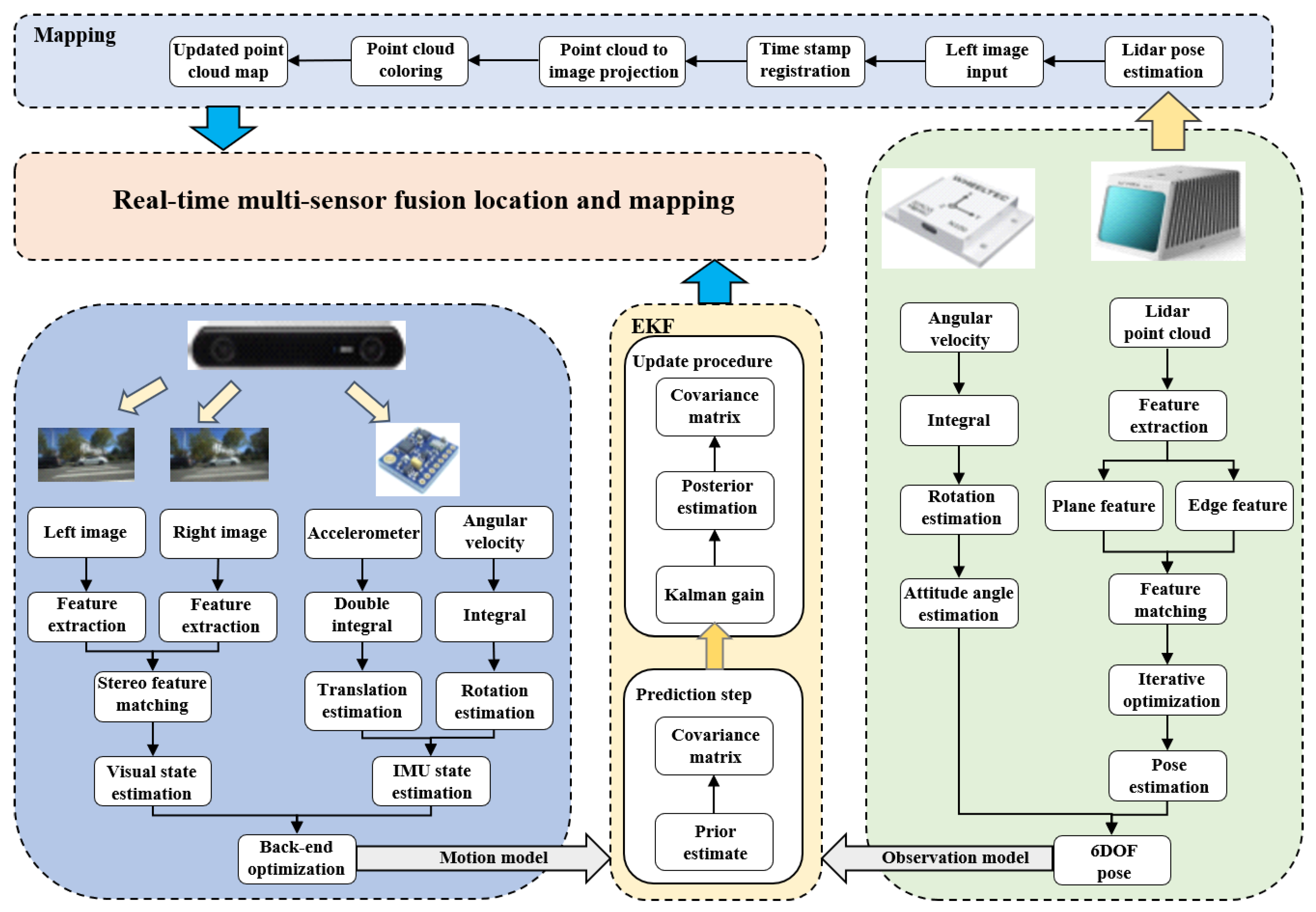
The system in this study is divided into two main parts, as illustrated in Figure 2: multi-sensor fusion localization and three-dimensional RGB point-cloud mapping. The multi-sensor fusion localization section integrates pose estimations from the LiDAR odometry, IMU, and VIO. The LiDAR sensor processes the scanned point cloud to derive LiDAR odometry, while the IMU’s three-axis gyroscope provides angular velocity data for estimating the robot’s rotation. The combination of LiDAR odometry and IMU pose estimation yields the robot’s six degrees of freedom (DOF) pose. This pose serves as the input for the state model of the EKF system. To calibrate the estimated pose obtained from the state model, the VIO output from the visual system is used as the observation model. By utilizing the Kalman gain from both the state and observation models, the optimal system state can be estimated. In the three-dimensional RGB point-cloud mapping section, the Loam_Livox algorithm was utilized and further enhanced with point cloud coloring functionality. This enhancement enabled the output of RGB point clouds, resulting in real-time generation of three-dimensional RGB point-cloud maps of the surrounding environment.

The algorithm was implemented on the Ubuntu 18.04 LTS operating system with ROS Melodic and developed using the C++ programming language.

2.2.1. The Pose Estimations from Sensors

The LiDAR SLAM employed the Loam_Livox algorithm, which is specifically designed for Livox LiDAR. Loam_Livox [13] is capable of delivering real-time synchronized 20 Hz odometry output and map updates. It consists of five modules: point selection and feature extraction, iterative pose optimization, feature matching, odometry output, and map updates. The algorithm (https://github.com/hku-mars/loam_livox, accessed on 28 May 2022) takes raw point cloud data from the Livox as input and produces the vehicle’s pose and a point cloud map of the surrounding environment as output.

During the measurement process, the angular velocities in the three directions of the tracked vehicle are captured using a three-axis gyroscope within an IMU. Let ${\widehat{\omega }}_t$ denote the measured angular velocity from the gyroscope, which is prone to noise interference. Hence, the measured gyroscope value comprises the true value ${\omega }_t$, white noise $n_{\omega }$, and bias $b_{\omega }$ [27,28,29]. It is important to note that the white noise is assumed to follow a Gaussian distribution to accurately model the noise characteristics.

$$\left\{\begin{array}{c}{n}_{\omega }~N\left(0,{\sigma }_{n\omega }^2\right)\\ b_{\omega }~N\left(0,{\sigma }_{b\omega }^2\right)\end{array}\right.$$

(1)

The formula for the angular velocity with noise can be expressed as:

$${\widehat{\omega }}_t={\omega }_t+n_{\omega }+b_{\omega }$$

(2)

By considering two consecutive LiDAR frames as $f_k$ and $f_{k+1}$, with corresponding time intervals of $t_k$ and $t_{k+1}$, the gyroscope measurements can be pre-integrated. This pre-integration process involves integrating the measured gyroscope values over the time interval to obtain cumulative estimates of orientation and angular velocity.

$$R_{f_{k+1}}^{f_k}={\int }_{t_k}^{t_{k+1}}{R}_t^{f_k}\left({\widehat{\omega }}_t-n_{\omega }-b_{\omega }\right)dt$$

(3)

In the equation, $R_{f_{k+1}}^{f_k}$ represents the rotation estimation between two consecutive laser radar frames, while $R_t^{f_k}$ represents the rotation pose at time $t_k$.

In order to refine the LiDAR odometry and IMU state estimates, we utilized the ZED2 camera within the VIO-SLAM module to obtain a 6 DOF pose estimation for the vehicle. The VIO-SLAM algorithm provided by ZED SDK 4.0 comprises four main components: visual front end, IMU backend, optimization, and loop-closure detection. Figure 3 provides an overview of the fundamental process involved in pose estimation using ZED SDK 4.0.

2.2.2. Localization Using LiDAR–IMU–Vision Fusion Based on Extended Kalman Filter

In this study, we employed the “robot_localization” ROS package (https://github.com/cra-ros-pkg/robot_localization, accessed on 15 June 2022) to implement real-time localization through multi-sensor fusion. The LiDAR odometry and IMU state estimation served as inputs for the state model, while the VIO state estimation was used as the input for the observation model. By utilizing an EKF-based multi-sensor loosely coupled framework, we integrated the pose estimations from the LiDAR odometry, IMU, and VIO to enhance the robustness and accuracy of the overall pose estimation.

The EKF is a widely utilized optimization method that is employed to estimate the state of a system. It integrates prior information, including the system state model and observation model, with real observation data in order to obtain the optimal estimate of the system’s state. By continuously updating the state estimate and the estimated error covariance matrix, the EKF achieves an improved estimation of the state, leading to enhanced accuracy and stability of the estimate [30]. To effectively handle the system’s nonlinearity, the EKF algorithm divides the system into two steps: prediction and update. In the prediction step, the system’s state model is employed to forecast the state. Subsequently, in the update step, the observation model is utilized to bring the prediction closer to the actual state.

The state model and observation model are as follows:

$$\left\{\begin{array}{c}{x}_k=f\left(x_{k-1},u_k\right)+{\omega }_k\\ z_k=h\left(x_k\right)+v_k\end{array}\right.$$

(4)

In the equation, $x_k$ represents the state vector at time k, $u_k$ represents the input control quantity, ${\omega }_k$ represents the state noise, $f\left(·\right)$ is the nonlinear system state transition function. $z_k$ represents the observed state vector at time k, $v_k$ represents the observation noise, $h\left(·\right)$ is the observation state function. Assuming $h\left(·\right)$ and $v_k$ are Gaussian white noise, the magnitude of the noise follows a Gaussian distribution.

Assume that the motion noise is Gaussian white noise with a mean value of 0.

$${\omega }_k~N\left(0,Q_k\right)$$

(5)

Expand the state vector of the system using the first-order Taylor series approximation and expand the state model into a linear equation.

$$x_k\approx f\left({\widehat{x}}_{k-1},u_k\right)+{\nabla f}_x\left(x_{k-1}-{\widehat{x}}_{k-1}\right)+{\omega }_k$$

(6)

In the equation, ${\widehat{x}}_{k-1}$ represents the posterior estimate of the state vector at time $\mathrm{k}-1$, and ${\nabla f}_x\left(·\right)$ denotes the Jacobian matrix of the state model.

Assume that the observation noise is Gaussian white noise with a mean value of 0.

$$v_k~N(0,R_k)$$

(7)

Expand the observation vector of the system using the first-order Taylor series approximation and expand the observation model into a linear equation.

$${ z}_k\approx h\left({\widehat{x}}_k^{-}\right)+\nabla h_x\left(x_k-{\widehat{x}}_k^{-}\right)+v_k$$

(8)

In the equation, ${\widehat{x}}_k^{-}$ represents the a priori estimate of the state vector at time $k$, and ${\nabla \mathrm{h}}_x\left(·\right)$ is the Jacobian matrix of the observation model.

The formulas for the prediction part of the EKF algorithm can be derived as follows:

A priori estimation of the predicted state vector:

$${\widehat{x}}_k^{-}=f\left({\widehat{x}}_{k-1},u_k\right)$$

(9)

The covariance matrix of the a priori estimation of the predicted state vector:

$$P_k^{-}=\nabla f_x{P}_{k-1}\nabla f_x^T+Q_k$$

(10)

The formulas for the update part of the EKF algorithm can be derived as follows.

Calculating the Kalman gain:

$$K_k=P_k^{-}\nabla h_x^T{\left(\nabla h_x{P}_k^{-}\nabla h_x^T+R_k\right)}^{-1}$$

(11)

Obtaining the posterior estimation of the state variables by updating them using the observed values:

$${\widehat{x}}_k={\widehat{x}}_k^{-}+K_k\left(z_k-h\left({\widehat{x}}_k^{-}\right)\right)$$

(12)

Updating the covariance matrix to the posterior estimation covariance matrix of the state variables:

$$P_k=P_k^{-}-K_k\nabla h_x{P}_k^{-}$$

(13)

2.2.3. Point Cloud Mapping with RGB Color

In order to enable localization, navigation, and obstacle avoidance, the establishment of a high-precision point-cloud map is crucial. This can be achieved by processing the point cloud data obtained from LiDAR sensors, as well as the images captured by cameras. By integrating these data sources, it becomes possible to construct a point cloud map that includes RGB color information. Such a map offers detailed and comprehensive information regarding the surrounding environment, providing invaluable insights for the vehicle’s operations.

In the map building module, we have made enhancements to the Loam_Livox algorithm and incorporated coloring functionality for point cloud mapping. These improvements were implemented to achieve precise alignment between 3D point clouds and 2D images in outdoor settings, as well as to incorporate RGB color information into the point clouds. The following steps were undertaken to accomplish this: joint calibration of the LiDAR and camera, point cloud filtering, timestamp alignment, projection of the LiDAR point cloud onto the image coordinate system, and point-cloud coloring. These steps ensure accurate spatial registration and add visual richness to the resulting point cloud map.

To achieve joint calibration between the LiDAR and camera, we utilized the open-source software called livox_camera_lidar_calibration available at (https://github.com/Livox-SDK/livox_camera_lidar_calibration, accessed on 6 August 2022). This software is specifically designed for the calibration of Livox LiDAR and cameras. The calibration process involved several steps, including intrinsic parameter calibration of the camera, acquisition of calibration data, and computation of the extrinsic parameters between the camera and Livox. The distinctive non-repeating scanning feature of Livox aided in accurately locating corners within high-density point clouds. This contributed to better calibration results and improved the fusion effect of the LiDAR-camera system.

To maintain real-time performance of the coloring process, it is essential to perform point cloud filtering due to the large number of points present in each frame. Filtering is primarily achieved through point selection, wherein certain points are excluded based on specific criteria. These criteria include identifying points on the edges or occluded points, points with excessively high or low intensities, and points with incident angles close to π or 0. Following the filtering step, feature extraction is performed by classifying the remaining points into two main categories: edge points and planar points. This classification is based on the local smoothness of the points and their intensity. By implementing these filtering and feature extraction techniques, computational efficiency is improved while ensuring accurate and reliable point-cloud coloring.

To achieve real-time alignment between each point cloud frame and its corresponding 2D image, the timestamps were synchronized between the LiDAR point cloud and the left image of the stereo camera. During data capture, the timestamps of each point cloud frame and image were recorded. Temporal registration between the point cloud and image occurred after pose estimation of the point clouds. Since the LiDAR point cloud has a lower frame rate (10 Hz) compared to the stereo camera (30 Hz), careful selection of images was necessary for alignment. When registering the image that corresponds to each point cloud frame, a time range of 15 ms before and after the point cloud timestamp was considered. From this time range, the image with the closest timestamp was selected. In instances where multiple images fell within the time range, the image with the closest timestamp to the point cloud frame was chosen for alignment. This approach ensured accurate temporal registration between the point cloud and its corresponding image.

To perform the projection of the LiDAR point cloud onto the image coordinate system and achieve point-cloud coloring, the following steps were undertaken. Firstly, the extrinsic parameters of the LiDAR and the left camera were utilized to transform each point from the processed point cloud. This transformation involved converting the point’s coordinates from the LiDAR coordinate system to the coordinate system of the left camera. Subsequently, the intrinsic parameters of the left camera were employed to project the point cloud from the camera coordinate system onto the image coordinate system (refer to Figure 4). As a result, the x and y coordinates of each point corresponded to the column and row of pixels on the image. By retrieving the corresponding RGB information from the pixel, the point cloud map with RGB color information was constructed. Finally, the edge points and planar points were aligned and merged on the map to continuously update the point cloud map and obtain the most recent colored point cloud map.

2.3. Experimental Design

The experiment was conducted at the Baima Teaching and Research Base of Nanjing Agricultural University, located in Nanjing, Jiangsu, China (refer to Figure 5). The experimental environment selected for this study was a pear orchard characterized by modern horticultural planting techniques. This environment was deemed highly suitable for tasks such as localization, mapping, and navigation of orchard vehicles. The pear trees within the orchard had an age range of 5–6 years and were in the stage of new shoot growth and young fruit development during the testing period. The tracked vehicle used for the experiment was operated through a remote-control handle and was maneuvered in various scenarios to carry out real-time localization and mapping tasks.

To evaluate the efficacy of the proposed multi-sensor fusion localization method, a total of eight tests were conducted in an outdoor orchard setting. These tests were designed to assess the performance of the method under different conditions and challenges that could impact accurate vehicle localization. Four tests involved different motion trajectories, varying the vehicle’s movement patterns throughout the orchard. The remaining four tests focused on different scenarios, creating diverse situations to examine the feasibility of the proposed method in challenging circumstances. These tests aimed to validate the effectiveness of the method in achieving accurate vehicle localization across a range of real-world scenarios.

2.3.1. Different Motion Trajectories

Vehicles frequently need to traverse intricate paths within orchards, necessitating the study of diversified trajectory navigation in complex scenarios. In this research, we conducted four motion trajectory tests, namely the “loop”, sharp turning, curve, and “N”-shaped trajectories.

The “loop” trajectory was implemented in a semi-structured pear orchard, featuring a relatively flat terrain and scaffolds in each row of trees for shape training. This trajectory facilitates closed-loop navigation in a comparatively simple environment, making it a widely used trajectory in practical vehicle applications.

On the other hand, the tests for sharp turning, curve, and “N”-shaped trajectories were carried out in sparsely planted pear orchards. In such scenarios, the pear trees in each row are widely spaced without any obstructions, enabling the vehicles to execute complex trajectory movements. The sharp turning trajectory allows the vehicle to make an approximate quarter turn. However, during the turning process, the visibility of frontal features significantly decreases, leading to increased instability and uncertainty in sensor data.

The curve trajectory involves guiding the vehicle along a flat curve between pear trees. Sometimes, the vehicle must alternate between different fruit trees, necessitating the testing of this particular trajectory. However, during curve navigation, the data obtained from sensors can be highly unstable, thereby augmenting the challenge of data processing for algorithms. The instability of features further complicates feature matching.

To verify the robustness and accuracy of our proposed approach in free-turning trajectory navigation, we instructed the vehicle to execute an “N”-shaped trajectory. The dynamically changing motion direction of this trajectory posed significant challenges.

2.3.2. Different Scenarios

The diverse planting methods used in orchards have resulted in variations in the orchard environment, increasing the overall diversity and complexity. Therefore, it is imperative to conduct studies examining the robustness and accuracy of vehicles in such diverse scenarios. Figure 6 illustrates the tests conducted in four different scenarios, including sparsely planted pear orchards, densely planted pear orchards, roads, and pond banks. In the sparsely planted pear orchards, the spacing between rows measures 4 m, while the spacing between columns measures 3 m. Conversely, the densely planted pear orchards have a row spacing of 2.8 m and a column spacing of 1.5 m. These scenes possess distinct complexities and characteristics, posing various challenges to the precise localization of vehicles.

In sparsely planted pear orchards, the spacing between pear trees is generally consistent, and the ground is relatively well-maintained. The large spacing between trees and the specific pruning of branches and leaves make these orchards suitable for mechanized management. Each row of pear trees is shape-trained using a scaffold, making it impossible to drive across rows. Consequently, vehicles can only travel in straight lines between columns.

Densely planted pear orchards, on the other hand, have closely spaced trees with narrow row spacing. This results in more branches and leaves between rows, which increases occlusion and poses challenges in feature extraction and matching for multi-sensor systems.

The road scene involves driving on the roads within the orchard, typically characterized by a flat surface with pear trees planted on both sides. In the frontal view of the vehicle, the road appears open and contains fewer distinguishable features. However, the side view of the road presents numerous objects with distinctive features, leading to an imbalance in the number of features between the two directions.

When the vehicle moves along the bank of a pond, there are different scenes on each side. On one side is the pond, which offers a wide field of vision with minimal distinctive objects. The reflectance of light on the water surface further complicates data collection, reducing its reliability. On the side with fruit trees, there are many distinctive objects and diverse structures, providing abundant sensor data. This results in an imbalance in the number of features between the two sides.

2.4. Evaluation Criteria

For localization accuracy evaluation, we utilized the high-precision inertial navigation system (INS-D-E1, Beijing BDStar Navigation Co., Ltd., Beijing, China). This system supports real-time kinematic (RTK) positioning, offering an impressive accuracy of up to 1 cm + 1 ppm.

In this experiment, we utilized the accuracy evaluation tool EVO (https://github.com/MichaelGrupp/evo, accessed on 25 September 2022) to comprehensively assess the performance of the system. This tool provided a comprehensive evaluation of the accuracy of the SLAM algorithms by measuring the absolute pose error (APE) values for both rotation and translation. The APE values are also referred to as absolute trajectory error (ATE) and serve as a metric to measure the global consistency of SLAM trajectories.

APE is based on two poses $P_{est,i}$ and $P_{ref,i}$ at timestamp i in SE (3), which can be calculated using the following formula:

$$E_i=P_{est,i}\ominus P_{ref,i}=P_{est,i}^{-1}{P}_{est,i}\in SE\left(3\right)$$

(14)

In the formula, $\ominus$ is an inverse composition operator that takes two poses and produces the relative pose. The value of high-precision inertial navigation system is used as reference.

In APE, the translation error is calculated by using the translation component of $E_i$, and the unit is in meters.

$${APE}_{trans,i}=‖trans\left(E_i\right)‖$$

(15)

The rotation error is calculated by utilizing the rotation component of $E_i$, and it is dimensionless.

$${APE}_{rot,i}={‖rot\left(E_i\right)-I_{3\times 3}‖}_F$$

(16)

Using the total error, considering rotational and translational errors, calculated with the full set $E_i$, unitless.

$${APE}_{rot,i}={‖rot\left(E_i\right)-I_{3\times 3}‖}_F$$

(17)

The root mean square error (RMSE) can be calculated using the absolute errors at all time points.

$$\mathrm{R}\mathrm{M}\mathrm{S}\mathrm{E}=\sqrt{\frac{1}{N}{\sum }_{i=1}^N{APE}_i^2}$$

(18)

In EVO, evo_res is a tool used for comparing the results of one or multiple evo_ape files. Therefore, relative posture error (RES) can be used for comparing APE values.

3. Results

3.1. Pose Accuracy of Different Motion Trajectories

Table 1. APE value comparison between the proposed multi-sensor fusion method and Loam_Livox of different motion trajectory.

Motion Trajectory	Method	Min	Max	Median	Mean	Std	RMSE
“Loop”	Fusion	0.0291	0.7720	0.0291	0.2890	0.1532	0.3271
	Loam_Livox	0.1762	1.2162	0.1762	0.4961	0.1999	0.5349
Sharp Turning	Fusion	0.1345	0.5539	0.2757	0.2801	0.0543	0.2853
	Loam_Livox	0.2258	0.8709	0.4466	0.4839	0.1633	0.5107
Curve	Fusion	0.0156	0.4792	0.0983	0.1205	0.0798	0.3734
	Loam_Livox	0.0259	0.7232	0.1733	0.1983	0.1181	0.5755
“N” shaped	Fusion	0.0059	0.6588	0.0955	0.1052	0.0688	0.3889
	Loam_Livox	0.0643	2.6056	0.4768	0.5993	0.3837	0.7257

compares the APE of trajectory tests between the proposed multi-sensor fusion method and the Loam_Livox algorithm. It is evident that the fusion method significantly improved accuracy across all trajectory tests. The RMSE decreased to nearly half of the values obtained with the Loam_Livox algorithm. Notably, the accuracy of the “N”-shaped motion trajectory improved the most. The fusion method achieved high accuracy in all motion trajectories, with an average RMSE of 0.3436, surpassing the Loam_Livox algorithm’s average RMSE of 0.5867.

3.1.1. “Loop” Trajectory in a Semi-Structured Pear Orchard

During the “loop” trajectory testing, the tracked vehicle followed a loop pattern inside the pear orchard. Figure 6f displays the designated area for the “loop” motion trajectory, which features large spacing between trees and scaffold-guided shape training. However, a ditch in the middle of the area allowed the tracked vehicle to pass through, albeit causing some bumps. The trajectory plots in Figure 7a illustrate that the motion trajectories of different methods were nearly overlapping. Nevertheless, Figure 7b highlights that the Loam_Livox algorithm exhibited larger positioning errors most of the time. In contrast, the proposed fusion method showcased higher pose accuracy, with a maximum APE difference of 0.3368. As indicated in Table 1, other error metrics for the fusion method were also smaller than those of the Loam_Livox algorithm, thus demonstrating the effectiveness of the proposed method in the challenging orchard environment.

3.1.2. Sharp-Turning Trajectory Inside a Sparsely Planted Pear Orchard

The ability to maneuver and turn effectively is crucial for tracked vehicles operating in large orchard environments, particularly when it comes to autonomous navigation. This study evaluates the efficacy of multi-sensor fusion localization in achieving precise turning motions between fruit trees, as depicted in Figure 8a. The results show that the proposed method in this paper accurately estimates the vehicle trajectory closer to the referential trajectory compared to the Loam_Livox method. In contrast, Loam_Livox exhibits significant errors during turning, leading to deviations in subsequent trajectory. The proposed fusion approach effectively corrects these errors and demonstrates significantly lower fluctuation compared to Loam_Livox. This finding is further supported by the error metrics in Figure 8c,d, which show that all error measurements for Loam_Livox are higher than those of the proposed method. Consequently, when tracked vehicles navigate between fruit trees, the proposed approach in this paper offers more accurate localization, thus enhancing autonomous navigation in orchard environments.

3.1.3. The Curved Trajectory Inside a Sparsely Planted Pear Orchard

In unstructured orchards, where there are no artificial obstructions between the trees, tracked vehicles often require curved motion trajectories. However, during curved motions, the tracking of feature points diminishes, leading to unstable tracking and increased errors in trajectory estimation. To evaluate the efficacy of the multi-sensor fusion method in such motions, Figure 9a was analyzed.

The results show that the Loam_Livox method initially exhibited substantial errors and later displayed noticeable trajectory deviations in the middle of large-angle curves. The LiDAR system had a significant impact on the overall system operation. Figure 9b demonstrates that our method initially had a higher peak, indicating poorer system stability, followed by a direct decrease. In contrast, the proposed approach in this paper utilizes data from a binocular camera and IMU sensor to correct errors in the central part of large-angle curves, subsequently resulting in smaller trajectory errors.

Furthermore, a comparison in Figure 9c,d reveals that the various error indicators of the Loam_Livox method are higher than those of the proposed approach. Therefore, when tracked vehicles navigate curved paths in an orchard environment, the proposed multi-sensor fusion approach provides more accurate positioning for the vehicle.

3.1.4. N-Shaped Trajectory in Sparsely Planted Pear Orchards

In large-scale orchards, tracked vehicles are tasked with various complex navigation assignments. To verify the robustness and accuracy of the proposed approach in unconstrained movement, the pose accuracy of a tracked vehicle executing an “N”-shaped trajectory was evaluated.

From Figure 10a, it is evident that the Loam_Livox method exhibits larger errors in corner tracking. The first corner shows a significant deviation, and while the error decreases during subsequent system operation, there is a sudden increase in error during the final turn. In contrast, the proposed approach in this paper leverages the benefits of multi-sensor fusion to correct trajectory errors at turning points. Boxplot analysis in Figure 10c demonstrates that the estimation errors obtained by the proposed approach in this study are contained within a smaller range. Additionally, other error indicators obtained by the proposed method are also smaller compared to those of Loam_Livox. Consequently, the proposed multi-sensor fusion approach in this paper effectively minimizes pose errors of tracked vehicles in complex environments like orchards.

3.2. Pose Accuracy of Different Scenarios

Tracked vehicles encounter various complex environments in orchards, and the diversity of these environments presents significant challenges to vehicle navigation and positioning. These challenges directly impact the effectiveness of autonomous navigation. To assess the performance of the proposed multi-sensor fusion method compared to Loam_Livox, the APE values for different scenarios are compared in

Table 2. APE value comparison between the proposed multi-sensor fusion method and Loam_Livox of different scenarios.

Motion Trajectory	Method	Min	Max	Median	Mean	Std	RMSE
Sparse Planting	Fusion	0.0047	0.5115	0.0632	0.0747	0.0563	0.0936
	Loam_Livox	0.0246	0.5928	0.1516	0.1626	0.0888	0.1853
Intensive Planting	Fusion	0.0083	0.4886	0.0567	0.0708	0.0582	0.0917
	Loam_Livox	0.0180	0.5446	0.0999	0.1094	0.0711	0.1305
Road	Fusion	0.0411	0.6047	0.1806	0.1878	0.0719	0.2011
	Loam_Livox	0.0761	2.8904	0.9832	1.0137	0.6065	1.1813
Bank of pond	Fusion	0.0088	0.5859	0.0780	0.0884	0.0581	0.1058
	Loam_Livox	0.0417	0.6756	0.2386	0.2512	0.1180	0.2776

. The fusion method exhibits increased accuracy in all scenarios, with particularly notable improvements in road scenarios. The road scenario demonstrates the highest increase in accuracy. Overall, the proposed method achieves an average RMSE of 0.1230 across all scenarios, outperforming the Loam_Livox method with an RMSE of 0.4436.

3.2.1. Sparse Planting in a Semi-Structured Orchard

To assess the accuracy of the proposed approach for sparse planting in a semi-structured orchard, straight-line movement experiments were conducted in this scenario.

As depicted in Figure 11a, both methods demonstrate high accuracy in this particular scenario. This result can be attributed to the consistent spacing between pear trees in the semi-structured orchard and the flat terrain, which facilitates stable movement of the tracked vehicle. The tracking and matching of feature points were successful, and since there were no turns during the movement, pose estimation errors remained small.

Figure 11c,d highlight the low error metrics attained by both methods. However, the proposed approach in this paper consistently outperforms the Loam_Livox method (Figure 11b) due to its utilization of multi-sensor fusion, which provides additional information for pose estimation and ultimately leads to higher accuracy. Thus, while both methods yield accurate pose estimation in the semi-structured pear orchard scenario, the proposed approach exhibits lower errors.

3.2.2. Intensive Planting in an Unstructured Orchard

The orchard primarily consists of densely planted pear trees without any artificial structures. In this scenario, the tracked vehicle is constrained to move only in straight lines. An evaluation was conducted to assess the accuracy and robustness of tracked vehicles navigating in this setting.

Figure 12a illustrates that the trajectories of both approaches closely overlap. The presence of numerous objects in the dense fruit tree rows provides ample feature points for successful feature matching. Despite the absence of structural objects, the increased data volume contributes to reduced pose estimation errors, thereby improving accuracy and robustness. However, compared to the sparse planting in the semi-structured orchard, this scenario exhibits greater fluctuation (Figure 12b).

Both approaches demonstrated excellent performance in terms of accuracy, as depicted in Figure 12c,d. The multi-sensor fusion method slightly outperformed the Loam_Livox method, highlighting its benefits for achieving higher accuracy in this scenario.

3.2.3. Road Scenario

To gauge the localization capability of the tracked vehicle on flat roads, the pose accuracy was tested in this scenario. Figure 13a reveals that the Loam_Livox method exhibits larger errors in this scenario, primarily due to two reasons. Firstly, the LiDAR’s limited FoV restricts its ability to accurately match feature points at turning points, resulting in increased errors that subsequently impact overall accuracy. Secondly, the tracked vehicle experiences significant vibrations when traversing on hardened ground, leading to decreased data accuracy from various sensors and consequently increasing errors.

A comparison of the errors in Table 2 with those in other scenarios reveals that the multi-sensor fusion approach significantly improves the accuracy in this scenario. Despite the increased pose estimation errors for both approaches, the proposed method demonstrates smaller errors in this environment.

3.2.4. Bank of Pond Scenario

In orchards, complex environments can sometimes occur. This particular scenario focuses on the area surrounding a pond adjacent to the fruit trees, as depicted in Figure 6a. Figure 14a illustrates the good overall localization performance of this approach, with the estimated trajectory closely matching the referential trajectory. However, Loam_Livox exhibits non-smooth changes in APE in the later stages of the experiment, accompanied by increased errors (Figure 14b). Despite this, the proposed method in this paper achieves a high level of pose accuracy, with an RMSE of 0.1059, indicating its reliability. The measurements obtained from the stereo camera and IMU effectively enhance the positioning accuracy of the LiDAR, making the proposed method applicable in semi-open scenes with fewer objects. Furthermore, the reflection from the water surface of the pond poses significant challenges in data acquisition. Analysis from Table 2 demonstrates that the integration of the binocular camera and IMU reduces the error range of the LiDAR, leading to improved positioning accuracy. Therefore, the utilization of a multi-sensor fusion method compensates for the limitations of individual sensors and achieves accurate and robust positioning in complex environments.

3.3. LiDAR Point-Cloud Mapping with RGB Color

Localization and mapping are crucial for enabling autonomous navigation in vehicles. To enhance the accuracy and efficiency of autonomous navigation and intelligent management of orchards, the utilization of three-dimensional LiDAR point-cloud maps with RGB colors can provide more detailed environmental information for tracked vehicles. To verify the feasibility of LiDAR point-cloud mapping with RGB color, tests were conducted in different scenarios within orchard environments, which corresponded to those described in Section 3.2.

The initial tests were performed in orchards with different planting modes. One scenario involved non-structured orchards with densely planted trees, while the other scenario involved semi-structured orchards with sparsely planted trees trained in a “Y”-shape. Figure 15a,d depict these two planting modes, showcasing their respective characteristics and the challenges encountered in constructing 3D RGB point-cloud maps. The non-structured trees, structured scaffolds, and the net above the canopy were accurately represented in the 3D RGB maps, with clear display of various colors. The results indicate that the maps possess relatively good quality. However, there is still room for improvement. The irregular sampling, non-repetitive scanning, and frame rates of the Livox point cloud may result in incomplete coverage of the entire tree, and the spacing between fruit trees and leaves can cause the laser beams to pass through the orchard without generating valid point clouds. Consequently, the observed tree shape on the map may not be complete.

The remaining tests focused on orchards with spatial constraints and specific features. One test was conducted on a road within the orchard, as illustrated in Figure 15g. In this scenario, both the road and the outer frame of the orchard were successfully constructed in the map. The spatial structure of the road surroundings was clearly displayed, and the coloring in the map was accurate. The other test took place between a pond and the orchard, as shown in Figure 15j. Weeds on the side of the orchard were successfully reconstructed; however, due to water absorption and laser reflection, the pond did not contain any points. Thus, LiDAR point-cloud mapping with RGB colors is applicable to such scenarios. Through these tests, the constructed maps demonstrate the robustness of the colorful mapping method in unstructured and diverse orchard environments.

Regarding the processing time in pose estimation and colorful mapping, our method required 75.01 ms for a frame of LiDAR point cloud, which represents a 2.79 ms increase for coloring compared to the original Loam_Livox algorithm [13]. This satisfies the requirement for real-time localization and mapping.

4. Discussion

For several decades, the precise positioning, mapping, and navigation of agricultural vehicles in orchard environments have been significant focal points in research. With the advancement and extensive investigation of SLAM technology, there has been a notable increase in research accomplishments in LiDAR SLAM, and the application scenarios have become increasingly intricate. The scanning range and data acquisition accuracy of LiDAR are well suited for constructing expansive scene maps. For instance, Loam_Livox [13] utilizes a single LiDAR and is able to effectively generate a three-dimensional point cloud map in a campus environment. The texture and geometric distribution of the surrounding scene can be vividly depicted, and it demonstrates commendable accuracy and robustness. However, orchard environments differ substantially from campus environments. Orchards lack high walls and are predominantly composed of short fruit trees, which possess irregular angles and gaps amidst their branches and leaves. These factors can diminish the data accuracy obtained by the LiDAR sensor. Consequently, the limitations of a single LiDAR hinder its adaptation to the complex scenes encountered in orchards.

In response to the above-mentioned problem, researcher [31] proposed an adaptive sensor fusion odometry framework based on SLAM that exhibits high efficiency. The framework primarily focuses on addressing the localization issue faced by agricultural unmanned ground vehicles in the absence of GNSS assistance. To achieve this, the framework employs a multi-sensor fusion approach, utilizing LiDAR, IMU, and monocular camera sensors. By incorporating three sub-odometries and integrating them based on environmental cues, the system’s adaptability and robustness are significantly improved. However, the unstructured objects and complexity of orchard scenes significantly diminish the reliability of geometric features in LiDAR SLAM. The unstructured characteristics of orchard scenes encompass irregular and unstable environmental information, such as the varying sizes of fruit trees, the multitude of tree branches, the dynamic movement of leaves, and the overlapping heights of leaves and branches [32,33]. These inherent characteristics result in uncertain and indescribable LiDAR data. Consequently, challenges arise in the processing, feature extraction, and matching of LiDAR point clouds, including insufficient and imperfect geometric feature extraction, as well as difficulties in matching.

The multi-sensor fusion method proposed in this paper enhances the accuracy of pose estimation by increasing the diversity of data captured using an IMU and stereo cameras. The loosely coupled approach also improves the robustness of the system, enabling it to effectively adapt to complex and challenging environments. Experimental results demonstrate that the proposed multi-sensor fusion method enhances data diversity, facilitating the effective utilization of the loosely coupled fusion framework to achieve highly accurate results even when LiDAR information is insufficient. This further enhances the stability and robustness of the system.

The LiDAR-generated point cloud lacks color information, and the environment map constructed using Loam_Livox is also devoid of color features. To address this limitation, this paper proposes algorithmic enhancements that leverage information acquired from multiple sensors. By combining the LiDAR point cloud with images captured by the stereo camera, RGB color information from the stereo camera is extracted and associated with each corresponding point in the point cloud. This integration facilitates the creation of an environment map that encompasses rich color features. Experimental results substantiate the effectiveness of our approach, showcasing an increased diversity of map information and providing a more comprehensive point cloud map for orchard management. As a result, our method furnishes reliable data for intelligent management.

However, there are still some limitations. The EKF model in the ROS package was used to fuse and filter the pose from multi-sensor, which updated and overwrote in every time buffer. Thus, the output pose of the EKF model was later than the input pose of the LiDAR, and the corresponding point cloud coordinates cannot be registered with the optimized pose through the time stamp. Therefore, we only registered the two sensors with time stamps when performing three-dimensional color mapping, to verify whether it can be used to establish the colorful orchard 3D map. In the future, we will rewrite the EKF algorithm to add a time label to every EKF calculation and calibrate the point cloud coordinates, and then compare the results with the current results.

Moreover, environmental disturbances, such as wind, can introduce outliers in the LiDAR-based point-cloud features during data acquisition. This phenomenon compromises the effectiveness of the acquired data and diminishes the available point cloud information. Subsequently, during point cloud processing, additional outliers are eliminated, resulting in reduced point cloud quantity and a decrease in the extracted geometric features. As a consequence, the availability of valid data for pose estimation is reduced, leading to a decline in accuracy and precision of the estimation. This situation also leads to poor convergence of iterative error data and an increase in errors in attitude calculation, ultimately weakening the system’s robustness.

In addition, the experimental results reveal that different motion trajectories have a greater impact on pose estimation error compared to variations in scenes. This effect arises due to the relatively narrow FOV of the utilized LiDAR, which hinders the matching of recognized feature points during complex trajectory operations. Moreover, the present LiDAR point-cloud mapping exhibits low density, which impairs the accurate identification of fruit tree features and hampers the creation of complete tree structures. To address these issues, future approaches will involve integrating multiple LiDAR systems to obtain point clouds with wider FOV and higher density. This integration aims to enhance the identification of fruit tree features and establish a more comprehensive orchard map. On this basis, we will conduct a more comprehensive and quantitative accuracy evaluation of LiDAR point-cloud colorful mapping.

5. Conclusions

This paper proposes a novel approach for real-time localization and mapping in unstructured outdoor orchard environments, eliminating the need for GNSS. To ensure accurate and robust pose estimation for tracked vehicles in complex orchards, the method integrates measurements from LiDAR odometry, an IMU, and a VIO within a loosely coupled multi-sensor fusion framework using an extended Kalman filter. This integration resolves individual sensor limitations. Simultaneously, the enhanced Loam_Livox algorithm is employed to create a point cloud map with RGB information of the surrounding environment. By combining precise positioning with the 3D RGB point-cloud map, the method achieves more accurate positioning for tracked robots, laying the groundwork for further advancements in autonomous navigation.

This method underwent evaluations in orchards featuring various complex motion trajectories and environmental conditions. Across all tests, the method consistently demonstrated a high level of accuracy and robustness in both positioning and mapping. However, during the testing phase, the limited FoV of the solid-state LiDAR impaired feature point tracking, particularly during turns, leading to reduced accuracy in the multi-sensor fusion localization. Furthermore, the current point cloud mapping has not been calibrated by the localization, and its density was insufficient for autonomous navigation at the level of individual trees. Therefore, future work should consider incorporating additional LiDARs and sensors and registering output pose data with sensor data within the multi-sensor fusion framework. This, in turn, will enable better integration of positioning and mapping results, facilitating practical autonomous navigation in smart orchard management.