Core Germplasm Construction Based on Genetic and Phenotypic Diversity of Buffalograss (Bouteloua dactyloides (Nutt.) Columbus) from the Great Plains of America

Abstract

Buffalograss is a valuable forage and turfgrass species native to the Great Plains of America. Utilization of genetic resources and conservation of germplasm rely on effective methods to differentiate and identify genetic differences quickly and at a relatively low cost. The lack of correlation between DNA marker-based genetic diversity and the geographic distance in buffalograss indicates that the interaction between genotype and environment needs to be evaluated. The objective of this study was to establish a core collection of buffalograss germplasm based on SRAP, then solidify the construction with important phenotypic traits. A total of 143 accessions were collected from 16 regions in 10 states of the U.S. A total of 1033 bands were scored from the 10 combinations of forward and reverse primers, of which 1031 were polymorphic within the accessions. After evaluating multiple clustering approaches, we determined that using symmetric distance (such as DMATCH, SM) in the hierarchical Ward’s method was the best clustering method, resulting in five groups. A least distance stepwise clustering approach using the simple match similarity coefficient was most efficient in creating core collections. Adding the phenotypic information and a final core collection size of 59 accessions was recommended to balance representativeness and diversity. We proposed a reverse power function for the percentage of accessions to be included in a core collection. We started at a high value for small numbers of accessions, and the percentage decreased as the accession number increased. then level off at 10% as the accession number reached 1000 and above.

1. Introduction

Buffalograss is a warm-season species native to the Great Plains of North America ranging from Central Mexico to Southern Canada. It is well adapted to arid climates with heavy soil textures and high pH. In addition to being a valuable forage species, it is well suited as a low-maintenance turfgrass for use as lawns, park grounds, roadsides, and golf courses due to its excellent drought tolerance and low growing habit. Its adaptability over this wide latitude was considered to be related to its ploidy levels, which vary from diploid (2n = 2x = 20) to tetraploid (2n = 4x = 40), pentaploid (2n = 5x = 50), and hexaploid (2n = 6x = 50) [1,2]. However, many of its biological traits are not well understood. To conserve germplasm, identify cultivars, and breed new cultivars using these genetic resources, techniques are needed to differentiate genetic differences of baffalograss quickly and at a relatively low cost.

Since the proposal of the core collection concept by Frankel and Brown [3], significant amounts of works have been done on this topic, as described in recent reviews [4,5,6]. This work can be grouped into two general areas. Firstly, there are ongoing discussions concerning the purposes, strategies, and methods of core collection construction for plants of different breeding systems, geographical distributions, and economic impacts [7,8,9,10]. Secondly, advancement in molecular biotechnology allows for reevaluation of the efficacy and diversity of existing collections [11,12].

Methods for identifying turfgrass cultivars and germplasm have evolved with the advancement of new technologies. Using phenotypes to study germplasm diversity and to identify cultivars is vulnerable to varying environmental conditions, and it is also time consuming because the approach relies on the investigation of large numbers of morphological traits. Isoenzyme and protein electrophoresis, especially those from seeds, have been used in the 1970s and 1980s for cultivar identification. Nuclear DNA markers, such as restriction fragment length polymorphisms (RFLPs) were used by Gulsen et al. [13] to assess genetic differences in buffalograss germplasm. However, using RFLPs is more difficult, time consuming and costly than using allozymes. New PCR technology has overcome the shortcomings of RFLP, leading to the use of random amplified polymorphic DNA (RAPD) technics in buffalograss in the 1990s [14,15]. A comparison of RAPD and allozyme techniques in buffalograss was provided by Peakall et al. [16]. Later, a sequence-related amplified polymorphism (SRAP) marker-based method was used to evaluate genetic diversity in germplasm and was found to be very effective in identifying new sources of alleles [13,17]. However, using the same method for both cytoplasmic and nuclear markers, Budak et al. [18] reported that there were no correlations between geographic distance and genetic differences among accessions of buffalograss.

The lack of correlation between DNA marker-based genetic diversity and the geographic distance in baffalograss indicates that the interaction between genotype and environment needs to be evaluated for breeding purposes as well as for constructing a more effective core collection of germplasms. The diecious breeding system in buffalograss, as well as its unique geographical distribution, present challenges for evaluating its germplasm collection, testing for genetic diversity, and evaluating its core collection. However, core construction of this species provides the opportunity to assess the existing models of core constructions for plants of different breeding systems.

The Great Plains where buffalograss is distributed have mostly been converted into farmlands since the second half of nineteenth century. Additionally, continuous breeding work is currently only centered in one state in the U.S. (https://www.usga.org/course-care/turfgrass-and-environmental-research.html) (accessed on 1 May 2023). Therefore, conserving buffalograss germplasm for future global use poses a significant challenge. The objective of this study was to establish a core collection of buffalograss germplasm based on SRAP, and then to solidify the construction with certain phenotypic traits that are important to turf quality.

2. Material and Methods

2.1. Plant Materials

One hundred and forty-three accessions of buffalograss were used for this study. The accessions were collected from 16 regions in 10 states of the Great Plains of the United States with vast climate differences (

Table 1. Accessions of buffalograss (Buchloe dactyloides (Nutt.) Engelm) from the Northern Plains of America.

Origin	Climate †	Accessions	Accession Code (Name)
Yellowstone National Park	Alpine (Dfc/Dfb), a.p ‡. 380 to 2000 mm	7	137 (C007_02AF), 138 (C007_03AM), 139 (C007_04AM), 140 (C031_02AF), 141 (C031_03AF), 142 (C031_04AF), 143 (C031_05AF)
East Wyoming	Semi-arid and continental (BSk), a.p. 300 mm	11	13 (A008_02BF), 14 (A008_03AF), 15 (A008_19AM), 16 (A008_21BM), 17 (A009_02AF), 18 (A009_07AF), 19 (A009_10AF), 20 (A010_10AF), 21 (A011_01AM), 22 (A011_02AM), 23 (A011_04AF)
Southeast North Dakota	Humid continental (Dfa/Dfb), a.p. 574 mm	1	108 (B001_01BM)
Central North Dakota	Humid continental (Dfb), a.p. 427 mm	5	1 (A002_00AM), 2 (A002_00AF), 3 (A002_01AM), 4 (A002_01AF), 43 (A028_01CF)
West North Dakota	Semi-arid (BSK), a.p. 381 mm	8	5 (A003_25AF), 6 (A004_01AF), 7 (A004_02AM), 8 (A005_01AM), 9 (A005_02CM), 10 (A006_03AF), 11 (A006_06AF), 12 (A006_07AF)
Central South Dakota	Humid continental (Dfa), a.p. 508 mm	11	38 (A024_01AM), 39 (A024_02BF), 40 (A025_00AM), 41 (A026_02AF), 42 (A026_03BF), 44 (A033_02AM), 45 (A033_03BF), 46 (A034_06AM), 47 (A034_07AF), 48 (A035_01AM), 109 (B030_01AM)
Northwest South Dakota	Steppe (BSk), a.p. 414 mm	5	33 (A017_01AF), 34 (A017_02AM), 35 (A019_01AM), 36 (A020_00AF), 37 (A021_00AM)
West Central Nebraska	Semi-arid (BSk), a.p. 350 mm	9	24 (A012_01AM), 25 (A012_02AM), 26 (A013_00AM), 27 (A013_00BM), 28 (A014_00AF), 29 (A014_00BF), 30 (A015_02AF), 31 (A015_07AF), 32 (A015_10BF)
Southeast Nebraska	Humid continental (Dfa), a.p. 800 mm	11	110 (B030_04AF), 113 (B037_06AF), 114 (B038_01AM), 115 (B038_02AF), 116 (B039_00AM), 117 (B039_02AF), 118 (B040_01AM), 119 (B040_02AF), 120 (B041_01AM), 121 (B041_03AF), 122 (B041_04AF)
Iowa	Humid continental (Dfa), a.p. 970 mm	2	111 (B036_01AF), 112 (B036_02AM)
North Central Kansas	Humid continental (Dfa), a.p. 930 mm	24	49 (A050_01AM), 50 (A051_01AF), 51 (A051_02AM), 52 (A051_03AF), 53 (A051_04BM), 54 (A052_02AF), 55 (A052_03AF), 56 (A053_01AF), 57 (A053_02AM), 58 (A054_01AF), 123 (B042_01AM), 124 (B043_01AM), 125 (B043_02AF), 126 (B043_03AF), 127 (B045_02AF), 128 (B045_03AF), 129 (B045_05BM), 130 (B046_02AM), 131 (B046_03AF), 132 (B046_04AM), 133 (B046_05AM), 134 (B046_06AF), 135 (B047_01AM), 136 (B049_01AF),
Southwest Kansas	Semi-arid steppe (BSk), a.p. 410 mm	14	59 (A055_01AM), 60 (A055_03BM), 61 (A055_04AF), 62 (A055_05BM), 63 (A055_07AF), 64 (A056_01AF), 65 (A057_01AF), 66 (A057_02BF), 67 (A057_05AF), 68 (A057_06AF), 104 (A072_02AF), 105 (A072_03AF), 106 (A073_01BM), 107 (A073_03AM)
Oklahoma	Humid subtropical (Cfa), a.p. 928 mm	7	69 (A058_02AF), 70 (A059_01AM), 71 (A059_02AM), 72 (A060_01AM), 73 (A060_05AM), 74 (A061_02BM), 75 (A062_01AM)
Northwest Oklahoma	Semi-arid (BSk), a.p. 438 mm	3	101 (A071_01AM), 102 (A071_05AF), 103 (A071_08AF)
Northeast New Mexico	Semi-arid (BSk), a.p. 363 mm	3	98 (A070_03AM), 99 (A070_05AM), 100 (A070_08AM)
Northwest Texas	Semi-arid (BSk), a.p. 520 mm	22	76 (A063_02AM), 77 (A063_03GM), 78 (A063_08AF), 79 (A064_01AM), 80 (A064_02AF), 81 (A064_03AF). 82 (A065_02AF), 83 (A065_03AM), 84 (A065_04AF), 85 (A066_01AF), 86 (A066_02AM), 87 (A066_03AM), 88 (A067_02AM), 89 (A067_05AM), 90 (A067_12CM), 91 (A067_16AM), 92 (A067_20BM), 93 (A068_01AM), 94 (A069_01AF), 95 (A069_03AF), 96 (A069_05AF), 97 (A069_06AF)

^† Climate type in the parenthesis is based on the Köppen system; ^‡ a.p., annual precipitation.

). Buffalograss materials were maintained in a greenhouse with temperatures of 30/15 °C (day/night) and a natural photoperiod. The light intensity was compensated to 400 µmol m⁻²s⁻¹ using metal halite lamps during the day. The accessions were hydroponically propagated in a greenhouse by placing two stolon cuttings in square plastic containers, each measuring 7 cm wide and 10 cm deep. The propagation process started in December 2013. Half strength Hoagland solution [19] was used and changed weekly. The research continued throughout the following years and ended in December 2018.

2.2. Field Phenotype Evaluation

Hydroponically propagated plant materials that developed healthy roots were transplanted to the Beijing Precision Agricultural Research Station (40.1778 N 116.3998 E, 38 m absl) in late April 2014. Each accession was planted in a 0.8 m by 0.8 m field plot with a wood frame. The frames were buried 5 cm below ground and 15 cm above ground and spaced 20 cm apart. The germplasm entries were arranged in randomized complete blocks with three replicates. The plants were watered weekly during the first month following transplantation. To avoid contamination, shoots spread outside the wood frames were routinely removed using scissors.

The research site has a monsoon-influenced continental climate (Köppen: Dwa) characterized by hot and humid summers and cold winters. The annual rainfall was 640 mm, with 60% occurring in July and August. The average summer high temperature was 31 °C, but the absolute high temperatures could exceed 40 °C. The average winter low temperature was −9 °C, with absolute lows of −20 °C. The soil was a silt loam (a coarse-silty, mixed, calcareous, Typic Calciustept), with pH 7.8, 2.1% organic matter, 0.75 g kg⁻¹ total Kjeldahl N, 36.8 g kg⁻¹ available P, and 120 g kg⁻¹ available K.

In this study, phenotype evaluation was focused on morphological traits such as height, tiller density, and stolon length. Measurements were conducted in June 2015. Five primary shoots were randomly selected for measurements of leaf length, leaf width, internode length, internode diameter, and canopy height. The leaf and internode were recorded from the bottom to top. The canopy height and leaf length were measured using a ruler with an accuracy of 0.5 mm, and the rest were measured with a caliper with a 0.01 mm accuracy.

2.3. DNA Extraction and SRAP-PCR

Genomic DNA was extracted in August 2015 from fresh leaf materials of each accession using the CTAB method outlined by Murray and Thompson [20]. All materials were maintained in the above-mentioned greenhouse. A total of 110 primer pairs following Li and Quiros [21], 11 forward and 10 reverse, were screened on buffalograss accessions. Ten final primer combinations were selected for use in this study based on their amplification consistency and band clarity (

Table 2. The SRAP primer combinations and sequences used in the amplification of genomic DNA of buffalograss (Buchloe dactyloides (Nutt.) Engelm) accessions.

Primer Combinations	Forward Sequence (5′-3′)	Reverse Sequence (3′–5′)	Polymorphic Bands
Me1-Em15	TGA GTC CAA ACC GGA TA	GAC TGC GTA CGA ATT TAG	161
Me1-Em16	TGA GTC CAA ACC GGA TA	GAC TGC GTA CGA ATT TGG	123
Me6-Em16	TGA GTC CAA ACC GGT AA	GAC TGC GTA CGA ATT TCG	64
Me9-Em18	TGA GTC CAA ACC GGT AG	GAC TGC GTA CGA ATT GGT	120
Me10-Em19	TGA GTC CAA ACC GGT TG	GAC TGC GTA CGA ATT CCG	98
Me5-Em1	TGA GTC CAA ACC GGA AG	GAC TGC GTA CGA ATT TAT	105
Me12-Em12	TGA GTC CAA ACC GGT CA	GAC TGC GTA CGA ATT ATG	77
Me10-Em15	TGA GTC CAA ACC GGT TG	GAC TGC GTA CGA ATT TAG	85
Me7-Em19	TGA GTC CAA ACC GGT CC	GAC TGC GTA CGA ATT CCG	84
Me2-Em15	TGA GTC CAA ACC GGA GG	GAC TGC GTA CGA ATT TAG	116
Total			1033
Average			103.3

). The PCR reaction solution was a 15 µL mixture containing 1.5 µL of PCR buffer (100 mM Tris-HCl at pH 8.3, 500 mM KCl, and 15 mM Mg Cl₂), 1.2 µL of DNA template, 1.5 µL of dNTPs (2.5 mM), 0.4 µL of MgCl₂ (2.5 mM), 2.0 µL of primer combinations (15 mM), 0.75 U of Taq polymerase, 0.8 µL of M13-FAM, and distilled water. The amplifications were carried out in a GeneAmp 9600 PCR system (ABI Co., Shanghai) using the following procedures: pre-denaturing at 94 °C for 5 min, 10 cycles of denaturing–annealing–extension (95 °C for 1 min, 35 °C for 1 min, and 72 °C for 1 min), another 40 cycles of denaturing–annealing–extension (95 °C for 1 min, 53 °C for 1 min, and 72 °C for 1 min), and a final extension at 60 °C for 30 min. The amplification products were sequenced using a 3730XL sequencer (ABI Co., Shanghai, China). The SRAP fragments were fractioned on polyacrylamide gels using a JY300C vertical gel apparatus (Junyi Oriental Co., Beijing, China). The gels were scanned using a BioSens apparatus (SC810B, Shanfu Scientific Co., Shanghai, China).

2.4. Ploidy Level Determination Using Flow Cytometry

Ploidy level determination work was conducted in April 2014. Six to eight young, fresh leaves from each accession of buffalograss germplasm maintained in the above-mentioned greenhouse were cut into 2–3 cm fragments and rinsed with distilled water, then digested and colored following the method described by Johnson et al. [1]. The ploidy levels were determined using a flow cytometer (Becton-Dickson, San Jose, CA, USA) with a known diploid cultivar ‘Density’ used as a standard. Mean DNA level content was based on 2000 nuclei. Each accession was analyzed using three separate extractions and flow cytometric runs. The sample and data were analyzed using Modfit 4.0 software.

3. Data Analysis

3.1. Genetic Diversity

The presence and absence of each SRAP fragment were coded as 1 and 0 in the data matrix, respectively. The GenALEX 6.5 program [22,23] was used to calculate the percentage of polymorphic loci (PPL). The locus frequency was also calculated from the data matrix and used to calculate Shannon’s diversity index as an estimation of the genetic diversity of accessions [24]:

$$H^{\prime }=-{\displaystyle \sum }_i^k{p}_i\log p_i$$

(1)

where k is the total number of polymorphic loci and p_i is the frequency of the i locus.

3.2. Accession Grouping

Different clustering methods were used to group the accessions. The first cluster analysis was performed using the unweighted pair-group (UPGMA, also known as average-linkage) method in the Numerical Taxonomy Multivariate Analysis System (NTSYS-pc version 2.1, Exeter Software, Setauket, NY, USA). The results were expressed as a dendrogram with a Jaccard coefficient. Using the same system, the ‘Flexible Method’ was also used for cluster analysis based on the simple match (SM) distance.

Alternatively, the SRAP data matrix was analyzed in SAS (SAS 9.4, SAS Institute, Cary, NC, USA), where the DMATCH distance (with the simple matching coefficient transformed into the Euclidean distance) was calculated using the PROC DSTANCE procedure. The results were then used for Ward’s minimum variance clustering using the PROC CLUSTER procedure.

Additionally, the SRAP allele data were subjected to STRUCTURE analysis using the admixture model (Structure Harvester 0.6.92) [25] in which the model estimation of K populations or genetic groups was conducted using the Bayesian approach, which uses a Markov Chain Monte Carlo (MCMC) process. The initial K values were set to 2 to 9, with 10 independent runs for each K value. A total of 100,000 Markov chains were operated following a burn-in period of 10,000 chains [26]. The final K value was based on the maximum change in the likelihood distribution ($\log \left\{Pr\left(X|K\right)\right\}$) (i.e., the ad hoc quantity related to the second order rate of change of the likelihood distribution). Group membership assignment was based on the probability of alleles occurring in a group [27].

3.3. Phenotype Analysis

Cluster analysis was conducted for the morphology traits of buffalograss using the Ward’s method in the CLUSTER procedure following the estimation of the covariance matrix following the ACECLUS procedure in SAS (SAS 9.4, SAS Institute, Cary, NC, USA).

3.4. Core Germplasm Construction

To construct a core germplasm collection for the 143 accessions, two strategies were tested in this study. The first approach was admixture-prioritized clustering (APC), as described by Hu et al. [28]. Starting from the lowest level of sorting, one of the two accessions with the highest amount of admixture was selected for the next round of clustering. If the two accessions in the lowest cluster level had the same amount of admixture, then the accession with the admixture of a lower frequency was selected for the next round of clustering. If the two accessions had same amounts of admixtures and frequencies, then one was randomly selected. The clustering process was repeated to generate cores with 45%, 40%, 35%, 30%, 25%, 20%, 15%, and 10% of the original accessions. The second approach used the least distance stepwise clustering (LDSC), as proposed by Wang et al. [29]. From the initial clustering, the accession with the shortest genetic distance in the lowest level of sorting was discarded before next round of clustering. The process was repeated to generate cores with 45%, 40%, 35%, 30%, 25%, 20%, 15%, and 10% of the original accessions. In this LDSC process, the genetic distance (GD) was calculated using one subtracted by the similarity coefficient (GS). Three different similarity coefficients were used, i.e., simple match (SM) similarity (GS_S), Sorensen-Dice similarity (GS_D), and Jaccard similarity (GS_J), expressed as follows:

GS_Sij = (a + d)/(a + b + c + d)

(2)

GS_Dij = 2a/[(a + b) + (a + c)]

(3)

GS_Jij = a/(a + b + c)

(4)

where a is the number of SRAP band occurring in both accessions i and j, b is the number of SRAP bands occurring in the i accession only, c is the number of SRAP bands occurring in the j accession only, and d is the number of SRAP band occurring neither in accessions i nor j.

Genetic diversity parameters H’ and PPL, as well as the amount of admixtures in the core collections at each step of the clustering were compared to their values in the initial accession group. A core collection was considered sufficient when at least 80% of PPL and 80% of admixtures from the original group were included in the new construction [28]. Principal coordinates analysis (PCoA) was conducted for the original accessions to determine the distribution of core accessions in the original accessions.

4. Results and Discussion

4.1. Genetic Diversity

A total of 1033 bands were scored from the 10 combinations of forward and reverse primers, of which 1031 were polymorphic within the accessions. The number of bands scored per primer ranged from 64 to 161 (average 103.1) (Table 2). The original accessions had a Shannon’s diversity index of 44.44, indicating that the 143 buffalograss accessions had diverse polymorphic loci.

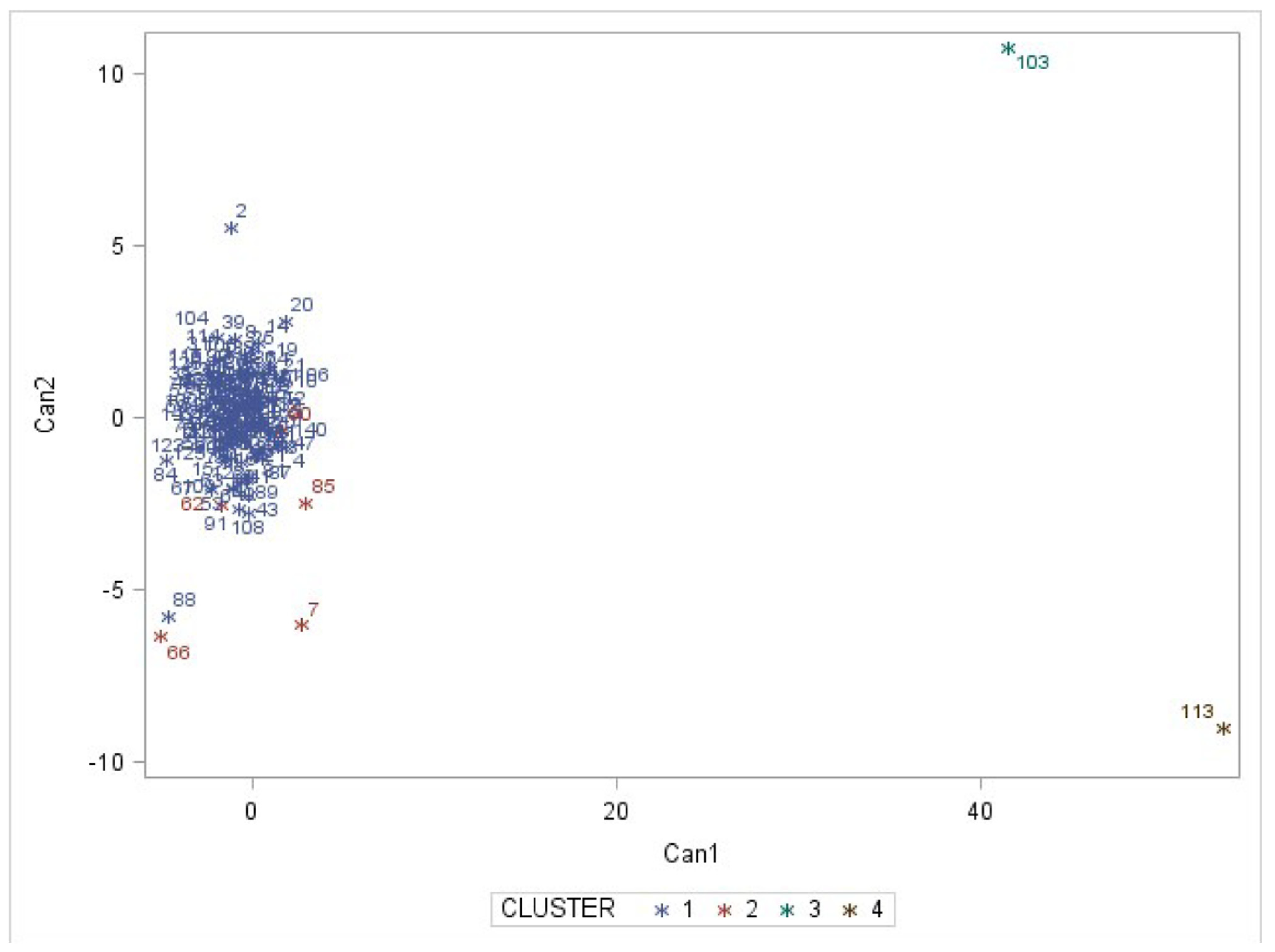
4.2. Accession Grouping

Using the UPGMA method to analyze the SRAP markers, the 143 accessions were clustered into four groups at the Jaccard’s distance coefficient of 0.33 (Figure 1). The first group contained 106 accessions, accounting for 74.13% of the total. The second group contained 22 accessions, accounting for 16.08% of the total. The third group contained 14 accessions, accounting for 9.79% of the total. The fourth group contained only one accession (A071-08AF). With a slight increase in similarity, significantly larger numbers of clusters were created, many of which had only one accession (Figure 1), indicating that this method did not have a strong grouping power.

Using the simple match coefficient for similarity distance in the Flexible method, the clustering resulted in five groups at a coefficient of similarity of 0.88 (Figure 2). This grouping resulted in three very small groups that had only 1 (C031-02AF), 2 (A002-00AF, A002-01AM), and 3 (A051-03AF, B040-01AM, and B040-02AF) accessions, respectively. As in the UPGMA method, a slight increase in the similarity coefficient resulted in the creation of many clusters containing only one accession.

When the DMATCH distance was used in the Ward’s clustering method, 5 clusters were identified at a semi-partial R-square value of 0.017 (Figure 3). This clustering method showed a similar grouping result as the Flexible method above, both having a cluster consisting of two accessions (A002-00AF, A002-01AM). However, Ward’s clustering using the DMATCH distance did not result in as many small groups as occurred in the Flexible method. There were no significant increases in the number of clusters as similarity coefficient increased (decreases in semi-partial R²), indicating that this grouping approach was effective.

The pseudo t-test (possible clusters at local peak back by 1) and pseudo F-test (possible clusters at highest local change of F values) both indicated 5 possible clusters for the grouping (Figure 4a). This was further corroborated by the MCMC method (Figure 4b), which had a regional peak change of the frequency increase rate at K = 5 [26]. Therefore, five clusters were considered as a reasonable initial grouping. Furthermore, because the existence and absence of a locus in different accessions at the same time should be of equal importance in grouping, using symmetric distances (such as SM or DMATCH) to analyze binary data was expected to generate more meaningful clustering results than asymmetric distances (such as Jaccard’s distance) using the UPGMA method [23]. In other words, the 5 clusters generated from the Ward’s clustering method using the DMATCH distance were considered the optimal grouping of the 143 accessions of buffalograss in this study. Our results agree with Tamasauskas et al. [30], who compared different methods of clustering using similarity/dissimilarity distances for binary data.

Examination of the groupings indicated that the clustering results were not associated with geographical origins of the accessions globally, meaning that not all accessions from closer geographical distance were closely clustered. However, all three methods (UPGMA, Flexible, and Ward) had many cases where accessions from the same location (represented by the first three digits of the accession name) were grouped together at the lowest level of clustering. This was especially true for the Ward’s cluster method using DMATCH distance (Figure 3), where accessions from closer geographical distances were more likely grouped together than other methods, with a few exceptions. The ploidy levels of accessions ranged from 2x to 6x and were not correlated with geographical locations, as also shown by Budak et al. [18]. The results were not completely in disagreement with Budak et al. [17]. This is because, although each geographical region belongs to one climate in general, there are large variations in rainfall, temperatures, and soil conditions. For example, the annual average precipitation varies from 380 mm near Mammoth Hot Springs to 2000 mm in the southwestern areas of Yellowstone National Park (National Park Service, https://www.nps.gov) (accessed on 15 January 2023). In addition, the accessions also have different ploidy levels, which are correlated with geographical distances [1].

4.3. Phenotype Evaluation

The accessions showed a large variation in morphological characteristics. The average plant height varied from 8 cm to 29 cm with a mean of 17.2 cm. The tiller number per plant varied from 17 to 38 with a mean of 26.5 (

Table 3. Summary of important morphological traits related to turfgrass quality in 143 accessions of buffalograss (Buchloe dactyloides (Nutt.) Engelm.).

	Leaf Length (mm)					Internode Length (mm)					Canopy Height (cm)	Tiller Number
	1st	2nd	3rd	4th	5th	1st	2nd	3rd	4th	5th
Max.	25.50	24.30	28.70	25.40	28.60	8.50	8.10	7.00	7.60	7.20	29.2	10.0
Min.	6.60	6.20	5.90	7.30	7.10	0.96	0.86	0.79	0.80	0.88	8.4	2.0
Avg.	14.07	14.96	15.31	14.85	14.93	4.29	4.01	3.96	4.09	4.05	17.2	5.3
SD	4.05	4.35	4.73	4.07	4.06	1.60	1.38	1.30	1.36	1.34	4.6	1.04

). The principal component analysis of the morphological data showed that the first latent variable (Can1) was mainly explained by the plant internode length and canopy height, and the second latent variable (Can2) was explained by the 5th leaf length and canopy height (Figure 5). Essentially, the canopy height was positively correlated with the internode length and leaf length, particularly the 5th leaf (flag leaf), with simple correlation coefficients of 0.31 (p < 0.001) and 0.38 (p < 0.001), respectively. A high canopy may have been the result of long internodes and/or a long 5th leaf. However, the length of the leaves and internodes were not correlated. The clustering results showed that both accession 103 (A064-02AF) and 113 (A061-02BM) belonged to a group with short internodes (Can1), but accession 103 had a shorter 5th leaf than accession 113 (Can2) (Figure 6). On the other hand, accessions 66 (B40-01AM) and 88 (B49-01AF) had long internodes, a long 5th leaf, and the highest canopy (Figure 5).

Many traits are important in terms of turfgrass quality in buffalograss [31]. These include stress tolerance, growth habits, and morphological characteristics. Evaluating and identifying these traits are essential to the breeding process [32]. The results from this study agree with the finding reported by Barker [33] that the phenotypes of these traits are heavily influenced by environmental conditions at a given geographical location. Therefore, evaluation of these phenotypes in different geographical locations is necessary.

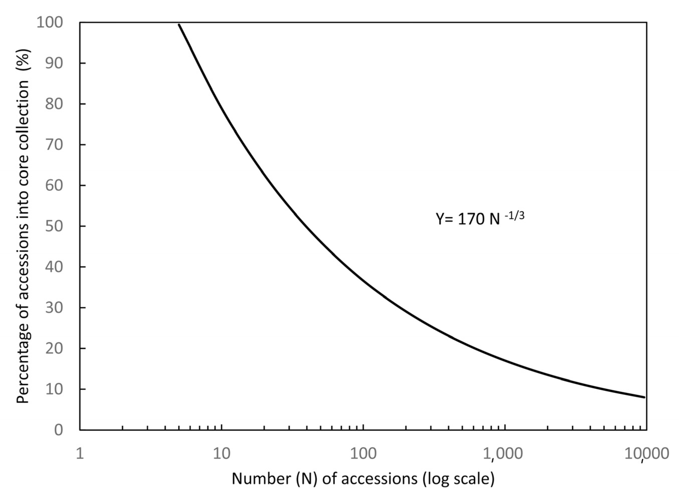
4.4. Core Germplasm Construction

Using the SM similarity coefficient with stepwise clustering resulted in higher admixture retention rates compared to Dice and Jaccard coefficients in both the LDSC and APC approaches (

Table 4. Evaluation of the core collection constructions using different clustering strategies and different similarity coefficients.

Core Size †	Admixture-Prioritized Clustering				Least Distance Stepwise Clustering
	PPL‡	Admixtures	Admixture Retained	H’§	PPL	Admixtures	Admixture Retained	H’
Original	99.81%	807	100.0%	44.44	99.81%	807	100.0%	44.44
S_45	82.87%	635	78.7%	32.37	87.71%	688	85.3%	35.30
S_40	80.83%	614	76.1%	30.50	86.06%	668	82.8%	33.39
S_35	77.73%	582	72.1%	28.61	81.12%	620	76.8%	30.78
S_30	75.80%	563	69.8%	26.77	77.83%	586	72.6%	28.30
S_25	72.99%	535	66.3%	24.34	73.96%	548	67.9%	25.48
S_20	67.96%	485	60.1%	21.45	68.25%	492	61.0%	22.33
S_15	58.37%	406	50.3%	17.64	61.57%	428	53.0%	18.61
S_10	51.21%	332	41.1%	11.04	51.89%	348	43.1%	13.67
D_45	82.19%	629	77.9%	32.49	86.64%	680	84.3%	33.12
D_40	80.83%	615	76.2%	30.84	83.93%	649	80.4%	31.00
D_35	77.73%	583	72.2%	28.62	81.12%	622	77.1%	28.94
D_30	75.70%	563	69.8%	26.49	76.57%	577	71.5%	26.43
D_25	71.35%	520	64.4%	24.29	71.44%	527	65.3%	23.47
D_20	66.60%	472	58.5%	20.91	66.21%	476	59.0%	20.90
D_15	60.70%	416	51.5%	17.68	59.73%	417	51.7%	17.03
D_10	50.73%	332	41.1%	13.01	48.40%	318	39.4%	12.15
J_45	84.70%	654	81.0%	32.81	86.64%	677	83.9%	32.89
J_40	81.32%	619	76.7%	30.58	84.22%	652	80.8%	31.06
J_35	79.57%	601	74.5%	28.92	80.83%	619	76.7%	28.74
J_30	75.67%	571	70.8%	26.65	76.28%	575	71.3%	26.26
J_25	72.22%	528	65.4%	24.00	71.25%	525	65.1%	23.31
J_20	67.47%	481	59.6%	21.18	65.54%	469	58.1%	20.29
J_15	61.18%	426	52.8%	17.75	59.83%	418	51.8%	16.94
J_10	50.63%	331	41.0%	12.99	48.40%	318	39.4%	12.15

^† S = simple match distance, D = Sorensen-Dice distance, and J = Jaccard distance. Subscripts indicate the percentage of the original accession number. ^‡ PPL, percentage of polymorphic loci. ^§ H’, Shannon’s diversity index.

). The LDSC approach also resulted in higher admixture retention and PPL rates than the APC approach at the same core size (Table 4). Using the LDSC approach and the SM similarity criterion, 57 accessions were selected at a core size of 40% (abbreviated as S-40). Although the same core size produced the same number of accessions, the actual accessions were different depending on the clustering strategies and similarity coefficients. Compared to other approaches, S-40 in the LDSC approach missed only two unique accessions which were deemed valuable based on genotype evaluations, i.e., 2 (A002-00AM) and 113 (A061-02BM). Accession A061-02BM had the shortest internode and longest 5th leaf, while accession A002-00AF had the highest number of tillers, longest internodes, and a very short 5th leaf. It is optimal for these two accessions to be included in the final core. When the final core collections were plotted with the original accessions in PCoA, it was apparent that the core collection was distributed in a pattern similar to the original accessions for both dimensions of PCoA (Figure 6). This indicates that the core collection represented the original accessions well.

The size of the core collection is affected by many factors. When the idea of core collection was proposed by Frankel and Brown [3], the core collection was suggested as an alternative to traditional conservation methods to reduce the cost of reserve genetic resources. The size should change due to continuous reception of new accessions, revision of groupings or affinities, and breeders’ priority. Sometimes, the collection is not used solely for conservation purposes, but rather as a basic breeding material. Therefore, for a breeder, the ultimate number of core collections will be based on the variability of traits of current and future interest, as well as analysis of climatic, ecological, and geographical information.

One of the cost factors of germplasm collection is the evaluation, which can be based on phenotypes as well as genotypes. When phenotypes are evaluated, many statistical parameters can be used, such as variability, niche width/variation [7], range retention index [34], and Shannon’s Index. In these cases, evaluation of a large number of accessions could be very expensive. Accordingly, 10% of the original accessions were proposed by Brown [7], as compared to the proportional and logarithmic approaches. For very large original accession numbers, such as the case of soybean (Glycine soja L.) germplasms (>15,500 accessions), 10% of random collection or multivariate strategies resulted in the best cores in terms of statistical variation or maximum range retention [35]. Therefore, core collection size may be affected by the breeding system of the species, as discussed by Brown [7]. In the case of outbreeding perennial ryegrass (Lolium perenne L.) in a relatively small geographical area, 86% of the original diversity requires 5% of the original accession based on phenotypes and the Shannon’s Index [36].

At the time when the proportional approach was proposed by Brown [7], DNA marker technology was rapidly developing, but still considered to be too expensive. However, more effective DNA marker technology such as SRAP can now be used to evaluate large amounts of accessions at a relatively low cost. To balance the representativeness and diversity, as well as for conservation purposes in places where buffalograss is not native, a larger core size is justified. In this study, the SRAP gene marker used for outbreeding species over a large geographical region seems to justify a higher percentage of core size [37]. For this reason, we propose a reverse power function strategy, where the entering percentage is high for small numbers of accessions and then decreases as the accession number increases until it approaches 1000, at which point the sample size levels off at approximately 10% (similar to the proposal by Brown [7]). This strategy is given in:

$$y=170 N^{-\frac{1}{3}}$$

(5)

where y is percentage of entries in the core collection and N is the number of original accessions (Figure 7). For example, using this equation, even for as many as 10,000 accessions, the sample size is 570 ($y$ = 5.7%).

5. Conclusions

As DNA marker technology becomes more affordable for the evaluation of large amounts of genetic resources over a large geographical region, SRAP has become economic and effective. This study has shown that SRAP is an effective method for genotyping buffalograss accessions from the Great Plains of America. The best approach to analyze the genetic diversity based on marker polymorphic bands demonstrated in this study was symmetric distance (such as DMATCH, SM) along with hierarchical clustering methods (such as Ward’s).

The least distance stepwise clustering approach using the simple match similarity coefficient was the most efficient in creating core collections. The efficacy of this method was evaluated using genetic diversity based on Shannon’s diversity index from the gene frequency. Phenotype evaluation and verification added extra information in understanding the affinity and diversity of original accessions. When the phenotypic information was added at a particular location in the genotypic clustering, a final core collection size of 59 was determined from the original 143 accessions. The resulting core collection had a balanced representativeness and diversity.

With all things considered, such as the cost, the purpose of collection, geographical variability, size, species’ breeding systems, and accessibility to wild resources, we proposed a new sampling strategy: the reverse power function. This sampling approach prioritizes a small number of accessions with a relative higher percentage of representation in the core collection. As the total number of accessions increases, the percentage decreases according to the reverse power function, approaching a level of 10% as the total accession number reaches 1000 and above.

References

1. Johnson, P.G.; Riordan, T.P.; Arumuganathan, K. Ploidy level determinations in buffalograss clones and populations. Crop Sci. 1998, 38, 478–482. [Google Scholar] [CrossRef]
2. Johnson, P.G.; Kenworthy, K.E.; Auld, D.L.; Riordan, T.P. Distribution of Buffalograss Polyploid Variation in the Southern Great Plains. Crop Sci. 2001, 41, 909–913. [Google Scholar] [CrossRef]
3. Frankel, O.H.; Brown, A.H. Current plant genetic resources—A critical appraisal. In Genetics: New Frontiers, Proceedings of the XV International Congress of Genetics, New Delhi, India, 12–21 December 1984; Oxford & IBH Publishing Co.: New Delhi, India, 1984; pp. 3–13. [Google Scholar]
4. Davies, L.R.; Allender, C.J. Who is sowing our seeds? A systematic review of the use of plant genetic resources in research. Genet. Resour. Crop Evol. 2017, 64, 1999–2008. [Google Scholar] [CrossRef]
5. Pascual, L.; Fernández, M.; Aparicio, N.; López-Fernández, M.; Fité, R.; Giraldo, P.; Ruiz, M. Development of a Multipurpose Core Collection of Bread Wheat Based on High-Throughput Genotyping Data. Agronomy 2020, 10, 534. [Google Scholar] [CrossRef]
6. Pathirana, R.; Carimi, F. Management and Utilization of Plant Genetic Resources for a Sustainable Agriculture. Plants 2022, 11, 2038. [Google Scholar] [CrossRef]
7. Brown, A.H.D. Core collections: A practical approach to genetic resources management. Genome 1989, 31, 818–824. [Google Scholar] [CrossRef]
8. Egan, L.M.; Conaty, W.C.; Stiller, W.N. Core Collections: Is There Any Value for Cotton Breeding? Front. Plant Sci. 2022, 13, 895155. [Google Scholar] [CrossRef]
9. Raturi, D.; Chaudhary, M.; Bhat, V.; Goel, S.; Raina, S.N.; Rajpal, V.R.; Singh, A. Overview of developed core and mini core collections and their effective utilization in cultivated rice and its related species (Oryza sp.)—A review. Plant Breed. 2022, 141, 501–512. [Google Scholar] [CrossRef]
10. Brown, A.H.D. The case for core collections. In The Use of Plant Genetic Resources; Brown, A.H.D., Frankel, O.H., Marshall, D.R., Williams, J.T., Eds.; Cambridge University Press: Cambridge, UK, 1989; pp. 135–156. [Google Scholar]
11. Cuevas, H.E.; Prom, L.K. Assessment of molecular diversity and population structure of the Ethiopian sorghum [Sorghum bicolor (L.) Moench] germplasm collection maintained by the USDA-ARS National Plant Germplasm System using SSR markers. Genet. Resour. Crop Evol. 2013, 60, 1817–1830. [Google Scholar] [CrossRef]
12. Reeves, P.A.; Tetreault, H.M.; Richards, C.M. Bioinformatic Extraction of Functional Genetic Diversity from Heterogeneous Germplasm Collections for Crop Improvement. Agronomy 2020, 10, 593. [Google Scholar] [CrossRef]
13. Gulsen, O.; Sherman, R.C.; Vogel, K.P.; Lee, D.J.; Baenziger, P.S.; Heng-Miss, T.M.; Budak, H. Nuclear genome diversity and relationships among naturally occurring buffalograss genotypes determined by sequence-related amplified polymorphism markers. HortScience 2005, 40, 537–541. [Google Scholar] [CrossRef]
14. Huff, D.R.; Peakall, R.; Smouse, P.E. Rapd variation within and among natural populations of outcrossing buffa-lograss [Buchloë dactyloides (nutt.) Engelm.]. Theor. Appl. Genet. 1993, 86, 927–934. [Google Scholar] [CrossRef]
15. Wu, L.; Lin, H. Identifying Buffalograss [Buchloe dactyloides (Nutt.) Engelm.] Cultivar Breeding Lines Using Random Amplified Polymorphic DNA (RAPD) Markers. J. Am. Soc. Hortic. Sci. 1994, 119, 126–130. [Google Scholar] [CrossRef]
16. Peakall, R.; Smouse, P.E.; Huff, D.R. Evoluationary implications of allozyme and RAPD variation in diploid populations of dioecious buffalograss Buchloe dactyloides. Mol. Ecol. 1995, 4, 135–147. [Google Scholar] [CrossRef]
17. Budak, H.; Shearman, R.C.; Gulsen, O.; Dweikat, I. Understanding ploidy complex and geographic origin of the Buchloe dactyloides genome using cytoplasmic and nuclear marker system. Theor. Appl. Genet. 2005, 111, 1545–1552. [Google Scholar] [CrossRef]
18. Budak, H.; Shearman, R.C.; Parmaksiz, I.; Gaussoin, R.E.; Riordan, T.P.; Dweikat, I. Molecular characterization of buffalograss germplasm using sequence-related amplified polymorphism markers. Theor. Appl. Genet. 2004, 108, 328–334. [Google Scholar] [CrossRef]
19. Hothem, S.D.; Marley, K.A.; Larson, R.A. Photochemistry in hoagland’s nutrient solution. J. Plant Nutr. 2003, 26, 845–854. [Google Scholar] [CrossRef]
20. Murray, M.G.; Thompson, W.F. Rapid isolation of high molecular weight plant DNA. Nucleic Acids Res. 1980, 8, 4321–4326. [Google Scholar] [CrossRef]
21. Li, G.; Quiros, G.L.F. Sequence-related amplified polymorphism (srap), a new marker system based on a simple pcr reaction: Its application to mapping and gene tagging in brassica. Theor. Appl. Genet. 2001, 103, 455–461. [Google Scholar] [CrossRef]
22. Peakall, R.O.D.; Smouse, P.E. genalex 6: Genetic analysis in Excel. Population genetic software for teaching and research. Mol. Ecol. Notes 2006, 6, 288–295. [Google Scholar] [CrossRef]
23. Peakall, R.; Smouse, P.E. GenAlEx 6.5: Genetic analysis in Excel. Population genetic software for teaching and research—An update. Bioinformatics 2012, 28, 2537–2539. [Google Scholar] [CrossRef] [PubMed]
24. Hennink, S.; Zeven, A.C. The interpretation of Nei and Shannon-Weaver within population variation indices. Euphytica 1991, 51, 235–240. [Google Scholar] [CrossRef]
25. Pritchard, J.K.; Stephens, M.; Donnelly, P. Inference of population structure using multilocus genotype data. Genetics 2000, 155, 945–959. [Google Scholar] [CrossRef] [PubMed]
26. Evanno, G.; Regnaut, S.; Goudet, J. Detecting the number of clusters of individuals using the software structure: A simulation study. Mol. Ecol. 2005, 14, 2611–2620. [Google Scholar] [CrossRef]
27. Earl, D.A.; vonHoldt, B.M. Structure Harvester: A website and program for visualizing STRUCTURE output and implementing the Evanno method. Conserv. Genet. Resour. 2012, 4, 359–361. [Google Scholar] [CrossRef]
28. Hu, J.; Zhu, J.; Xu, H.M. Methods of constructing core collections by stepwise clustering with three sampling strategies based on the genotypic values of crops. Theor. Appl. Genet. 2000, 101, 264–268. [Google Scholar] [CrossRef]
29. Wang, J.C.; Hu, J.; Xu, H.M.; Zhang, S. A strategy on constructing core collections by least distance stepwise sampling. Theor. Appl. Genet. 2007, 115, 1–8. [Google Scholar] [CrossRef]
30. Tamasauskas, D.; Sakalauskas, V.; Kriksciuniene, D. Evaluation Framework of Hierarchical Clustering Methods for Binary Data. In Proceedings of the 12th International Conference on Hybrid Intelligent Systems (HIS), Pune, India, 4–7 December 2012; pp. 421–426. [Google Scholar] [CrossRef]
31. Abeyo, B.; Shearman, R.C. Buffalograss (Buchloe dactyloides) turfgrass performance and seed yield characteristics. Int. Turfgrass Soc. Res. J. 2009, 11, 519–531. [Google Scholar]
32. Johnson, P.G.; Riordan, T.P.; Johnson-Cicalese, J. Low-mowing tolerance in buffalograss. Crop Sci. 2000, 40, 1339–1343. [Google Scholar] [CrossRef]
33. Barker, R.E. Statistics of cultivar discrimination: Are differences real. Intern. Turfgrass Soc. Res. J. 1997, 8, 215–227. [Google Scholar]
34. Diwan, N.; McIntosh, M.S.; Bauchan, G.R. Methods of developing a core collection of annual Medicago species. Theor. Appl. Genet. 1995, 90, 755–761. [Google Scholar] [CrossRef]
35. Oliveira, M.F.; Nelson, R.L.; Geraldi, I.O.; Cruz, C.D.; de Toledo, J.F.F. Establishing a soybean germplasm core collection. Field Crops Res. 2010, 119, 277–289. [Google Scholar] [CrossRef]
36. Charmet, G.; Balfourier, F. The use of geostatistics for sampling a core collection of perennial ryegrass populations. Genet. Resour. Crop Evol. 1995, 42, 303–309. [Google Scholar] [CrossRef]
37. Rao, V.R.; Hodgkin, T. Genetic diversity and conservation and utilization of plant genetic resources. Plant Cell Tissue Organ Cult. (PCTOC) 2002, 68, 1–19. [Google Scholar] [CrossRef]
Figure 1. Dendrogram showing cluster results of 143 Buffalograss (Bouteloua dactyloides (Nutt.) Columbus) accessions based on the Jaccard’s distance coefficient in the UPGMA method.
Agronomy 13 01382 g001
Figure 2. Dendrogram showing cluster results of 143 Buffalograss (Bouteloua dactyloides (Nutt.) Columbus) accessions based on the simple match coefficient for similarity in the Flexible method.
Agronomy 13 01382 g002
Figure 3. Dendrogram showing cluster results of 143 Buffalograss (Bouteloua dactyloides (Nutt.) Columbus) accessions based on the DMATCH distance in Ward’s method.
Agronomy 13 01382 g003
Figure 4. Statistical evaluation of clustering methods used for the 143 Buffalograss (Bouteloua dactyloides (Nutt.) Columbus) accessions. (a). Pseudo F-test and pseudo t-test results. (b). The second order rate of change of the likelihood distribution k group ( log { P r ( X | K ) } ).
Agronomy 13 01382 g004
Figure 5. Principal component analysis results of the morphological data for 143 Buffalograss (Bouteloua dactyloides (Nutt.) Columbus) accessions. The first latent variable (Can1) was mainly explained by the plant internode length and canopy height; the second latent variable (Can2) was explained by the 5th leaf length and canopy height. Accessions with 2n = 6x are represented by numbers 1−5, 8, 9, 12, 13, 17−19, 25, 32−34, 40, 43, 44, 47, 49−51, 53−56, 59, 62−68, 72, 74, 75, 80−87, 89−94, 96−98, 101, 102, 104, 108, 109, 113, 116, 119−121, 137−139, and 141−143. Accessions with 2n = 5x are represented by numbers 7, 11, 14, 60, 61, 69, 77−79, 105, 107, 117, 129, and 140. Accessions with 2n = 4x are represented by numbers 6, 10, 15, 16, 20−24, 26−29, 35−38, 41, 42, 45, 46, 48, 57, 58, 70, 71, 73, 76, 88, 95, 99, 100, 103, 106, 110−112, 114, 115, 122, 124−128, 130, and 132−136. Accessions with 2n = 3x are represented by numbers 39 and 118, while accessions with 2n = 2x are represented by numbers 30, 31, 52, 123, 131. Four color-coded numbers show the clustered groups of the accessions.
Agronomy 13 01382 g005
Figure 6. Principal coordinates analysis (PCoA) of 143 Buffalograss (Bouteloua dactyloides (Nutt.) Columbus) accessions showing representations by core accessions. The accessions with 2n = 6x are represented by numbers 1−5, 8, 9, 12, 13, 17−19, 25, 32−34, 40, 43, 44, 47, 49−51, 53−56, 59, 62−68, 72, 74, 75, 80−87, 89−94, 96−98, 101, 102, 104, 108, 109, 113, 116, 119−121, 137−139, and 141−143. Accessions with 2n = 5x are represented by numbers 7, 11, 14, 60, 61, 69, 77−79, 105, 107, 117, 129, and 140. Accessions with 2n = 4x are represented by numbers 6, 10, 15, 16, 20−24, 26−29, 35−38, 41, 42, 45, 46, 48, 57, 58, 70, 71, 73, 76, 88, 95, 99, 100, 103, 106, 110−112, 114, 115, 122, 124−128, 130, 132−136. Accessions with 2n = 3x are represented by numbers 39 and 118, while accessions with 2n = 2x are represented by numbers 30, 31, 52, 123, 131. The orange color denotes accessions included in the final core collection, while open circles are those not included.
Agronomy 13 01382 g006
Figure 7. A reverse power function strategy for sampling the original accessions as entry to core collection.
Agronomy 13 01382 g007