Abstract
Crop growth is often uneven within an agricultural parcel, even if it has been managed evenly. Aerial images are often used to determine the presence of vegetation and its spatial variability in field parcels. However, the reasons for this uneven growth have been less studied, and they might be connected to variations in topography, as well as soil properties and quality. In this study, we evaluated the relationship between drone image data and field and soil quality indicators. In total, 27 multispectral and RGB drone image datasets were collected from four real farm fields in 2016–2020. We analyzed 13 basic soil quality indicators, including penetrometer resistance in top- and subsoil, soil texture (clay, silt, fine sand, and sand content), soil organic carbon (SOC) content, clay/SOC ratio, and soil quality assessment parameters (topsoil biological indicators, subsoil macroporosity, compacted layers in the soil profile, topsoil structure, and subsoil structure). Furthermore, a topography variable describing water flow was used as an indicator. Firstly, we evaluated single pixel-wise linear correlations between the drone datasets and soil/field-related parameters. Correlations varied between datasets and, in the best case, were 0.8. Next, we trained and tested multiparameter non-linear models (random forest algorithm) using all 14 soil-related parameters as features to explain the multispectral (NIR band) and RGB (green band) reflectance values of each drone dataset. The results showed that the soil/field indicators could effectively explain the spatial variability in the drone images in most cases (R2 > 0.5), especially for annual crops, and in the best case, the R2 value was 0.95. The most important field/soil features for explaining the variability in drone images varied between fields and imaging times. However, it was found that basic soil quality indicators and topography variables could explain the variability observed in the drone orthomosaics in certain conditions. This knowledge about soil quality indicators causing within-field variation could be utilized when planning cultivation operations or evaluating the value of a field parcel.
1. Introduction
The smart farming concept calls for spatial knowledge about field and soil properties. Crop growth and development are not homogeneous within a field parcel, even if the field has been managed evenly. Terms such as “spatial variability” and “within-field variability” are commonly used to describe this situation [1]. Optical drone-based remote sensing of agricultural fields is an excellent tool to determine the spatial and temporal variations in crop stand properties. The reasons for within-field variability need to be considered to better understand the soil–crop system when cultivation operations are planned, and thus to control within-field variation, but also when the value of a field parcel is estimated. Often, spatial variations in crop growth and yield are related to variations in different chemical and physical soil properties (e.g., [2,3,4]). These properties are used to determine soil quality indicators, including the soil’s chemical (pH, soil organic carbon content (SOC), and nutrient content), physical (texture, penetration resistance, bulk density, and saturated hydraulic conductivity), and biological (number of earthworms and microbial biomass) components [5,6]. The relationships between variability in the measured yield and soil property/quality indicators have been studied by monitoring soil properties at the field scale, but this usually requires a large amount of sampling (e.g., [7,8,9,10]), making it time-consuming and laborious.
Remote sensing, either through satellite imagery or low-altitude drones (i.e., unoccupied aerial vehicles (UAVs)), has already been widely employed in different agricultural applications [11]. Low-cost commercial drones are usually used to collect spectral data to estimate different crop parameters, such as biomass [12,13] and nitrogen content [14,15], in order to predict crop yields [16,17,18] and identify weeds [19,20] or water stress in crops [21]. The popularity of drones is due to their flexibility and cost-efficiency in farm-scale surveys in comparison to satellite or terrestrial approaches [22].
In contrast to the large number of drone-based studies focusing on crop parameters, soil-related parameters have been less studied [23]. Recently, Diaz-Gonzalez et al. [5] reviewed remote sensing and machine learning techniques for soil quality indicator estimation, and found 22 studies on the topic. Various chemical, physical, and biological soil properties, as well as other crop management- and environment-related indicators such as topography, have been evaluated, but most of the studies utilized spectral data collected from satellites. A study with drones was conducted in China by Hu et al. [24] to estimate soil salinity using hyperspectral data and the random forest algorithm (RF). They achieved the highest correlation for a bare soil test site in comparison to a site with more vegetation. The capability of multispectral remote sensing to estimate SOC has also been studied [25,26]. Žížala et al. [25] compared different data sources and concluded that multispectral data collected from UAVs were a suitable and cost-effective alternative for SOC estimation in comparison to other data sources, such as satellite and aerial hyperspectral data. Khanal et al. [27] used aircraft to collect RGB and multispectral images from bare soil fields in a single day in the United States of America. They predicted soil properties using image data and machine learning and achieved a high correlation coefficient, for instance, for soil organic matter content (SOM).
In Finland, the on-farm use of drone imaging in crop production is increasing. Similarly, the use of soil quality assessments is strongly recommended to farmers to enable them to analyze the reasons for variations in soil properties that affect soil function and crop growth, and to plan and implement measures to manage within-field variation. The objectives of the present study were:
(i) To examine the relationship between multiannual drone orthomosaic datasets and commonly available soil and field indicators, including field topography, soil texture, organic matter content, penetration resistance, and soil structural properties, as determined via a simple Finnish soil quality assessment [28]; and
(ii) To study how well the available soil- and field-related indicators can explain spatial variability in agricultural fields observed from drone orthomosaic images.
We carried out this case study under real farm conditions to understand how aerial images and basic soil quality indicators can be used to explain the within-field spatial variation of a crop stand.
2. Materials and Methods
2.1. Experimental Fields
This study was conducted in four farm fields, of which two were located in Southern Finland, about 60 km west of Helsinki (i3 and i4, hemiboreal climate zone and growing zone I), and two were 500 km further north (l1 and l2, middle boreal climate zone and growing zone V), near the city of Oulu (Figure 1). Fields l1, l2, and i3 were relatively flat in comparison to field i4, where the difference between the minimum and maximum elevation was nearly 6 m (Table 1). Fields l1 and l2 were fine sandy soils that had 2.40% SOC content, and fields i3 and i4 were classified as loamy clay soils with an SOC content of 2.35–3.23% (in a 0–20 cm layer). All fields were managed evenly during the experiments, i.e., farming practices such as sowing and fertilizing were not expected to cause within-field variability. Precipitation varied greatly depending on the growing season, as shown in Appendix A.
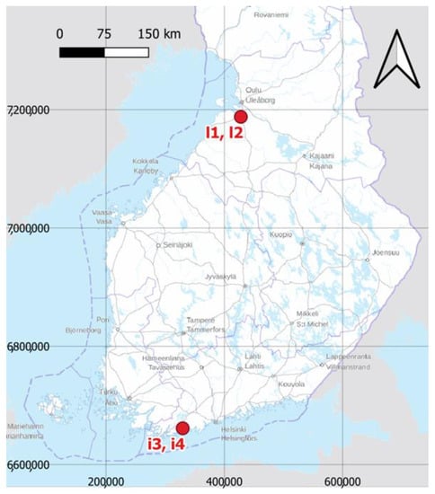
Figure 1.
The locations of the study fields in southern and northern Finland (ETRS-TM35FIN). Fields i3 and i4 were located in a hemiboreal climate zone and growing zone I, and fields l1 and l2 were located in a middle boreal climate zone and growing zone V [29,30].

Table 1.
Surface area, minimum and maximum elevation (Height System: N2000), and growing zones [30] of the four experimental fields.
2.2. Measurements and Determinations
2.2.1. Drone Data Collection
Multiannual drone data were collected in the experimental fields during 2016–2020 (Table 2). Data were collected using RGB multispectral and hyperspectral cameras (Table 2). The two multispectral cameras included a band in the green (central wavelength: 550–560 nm), red (660–668 nm), red-edge (717–735 nm), and near-infrared spectral range (790–840 nm), and the Micasense Altum camera included an additional blue band (475 nm). The hyperspectral FGI2012b camera [31,32] collected 36 spectral bands, but only the four bands corresponding to those of other multispectral cameras were used in this study. A commercial drone (DJI Phantom 4) and two in-house drones, a hexacopter (FGI Hexa; see details, e.g., [33]) and a quadcopter (FGI Quadro; see details, e.g., [34]), were used as platforms.
Table 2.
Overview of drone data: data collection date (Date), camera type: RGB or multispectral (MS) (* the camera collected 36 bands but only four of them were used in this study), sensor model, drone, original ground sample distance at the ground level (GSD), and crop type in the field during data collection.
The data were collected to produce geometrically accurate and radiometrically uniform orthomosaics, where the variability in the field was only related to the object itself, not to the measurement procedure. The flights were planned according to the following principles: minimum side overlaps were set at 70%, and forward overlaps at 80%; the flight heights were set to 120–140 m; data were collected within three hours from solar noon; and the direction of flight lines was mainly selected to be nearly parallel with the solar azimuth angle. Additionally, ground control points were placed and measured to support geometric processing, and reference reflectance panels were placed to support radiometric processing. Flight height and various sensor parameters resulted in ground sample distances (GSD) of 2–14 cm. The crops cultivated during the data collection stage (Table 2) were silage grass (a mixture of typical silage grass containing timothy (Phleum pratense L.) and other grasses (e.g., Festuca pratensis (Huds.) Darbysh. Lolium perenne L., Lolium multiflorum Lam., and Dactylis glomerata L.), and legumes such as red clover (Trifolium pratense L.)), spring barley (Hordeum vulgare L.), rapeseed (Brassica napus L. ssp. oleifera (Moench.) Metzg.), winter wheat (Triticum aestivum L.), and pea (Lathyrus oleraceus Lam.).
2.2.2. Drone Data Processing
Drone data were geometrically processed using photogrammetry and structure-from-motion (SfM) algorithms, described, for instance, by Wu et al. [35], and for the FGI2012b camera data, the processing followed the pipeline described by Näsi et al. [36]. The drone data were mainly collected under stable illumination conditions, but if partially cloudy images occurred, they were excluded from the orthomosaic calculations to produce radiometrically uniform orthomosaics (Figure 2). Orthomosaics were additionally converted to reflectance values, utilizing reference panels with nominal reflectance values of 0.05, 0.10, and 0.50 to ensure that different datasets were comparable. In the next phases of this study (statistical analysis), only one band of each camera was used as there was no significant difference between the results for each band. From the RGB datasets, the green band was selected, and from the MS datasets, the NIR band was selected. The spectral responses for all RGB cameras were typical of consumer cameras; additionally, the center wavelength was close to 530 nm, and the FWHM (full width at half maximum) was 100 nm [37,38]. The center wavelengths of the NIR bands were 790–840 nm, and the FWHM was 10–40 nm. The selected bands were considered to best indicate the amount of vegetation in the fields. The crops in the fields were in different growth stages, and especially in datasets collected before mid-June in I2, i3, and i4, the canopy was in the early growth stage, and bare soil was dominant instead of crop vegetation (Figure 2).
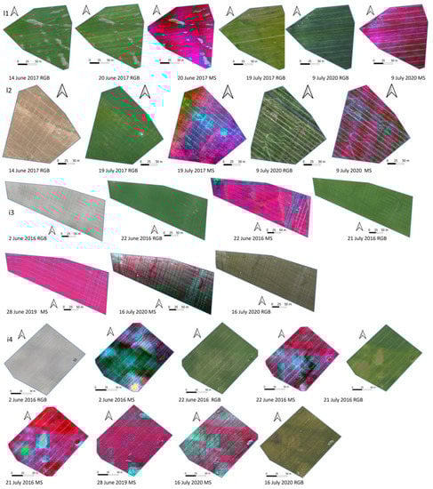
Figure 2.
Orthomosaics generated from drone images for all real farm fields in order of the data collection date (Table 2). Color infrared (CIR) mosaics were visualized from MS.
2.2.3. Soil and Topography Data Collection
The soil properties of the four fields were determined from different sampling points in 2019–2021. This was carried out soon after sowing or late in autumn in order to ensure suitable soil moisture conditions for conducting measurements and observations. Sampling points (10–12 per field) were chosen based on the drone orthomosaics of the fields to find spatial variation. Figure 3 shows the distribution of the soil sampling points of all the fields. From these points, the soil penetrometer resistance was determined as the median of 15 measurements (7.5 m × 7.5 m area) from a depth of 0–50 cm with 1 cm intervals, using a hand penetrometer from Eijkelkamp. The size of the cone used in the measurements was 1.0 cm2 (angle: 60 deg). In the present study, mean values of 5–15 cm and 20–40 cm were used in the analyses.
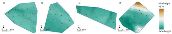
Figure 3.
Locations of soil sampling points marked with red dots, and the topography (DTM produced from drone datasets) is visualized using a color scale (the minimum height for each parcel is presented in Table 1) and contour lines with 1 m intervals for the four study fields (l1, l2, i3, and i4).
From the same sampling points, at which the penetrometer resistance was determined, soil samples were taken from a topsoil layer of 0–20 cm to determine the soil texture (sieving and pipette methods, ISO 11277:2009) and organic carbon content (volatile solids method and oven-drying at 550 °C). The physical quality of soil from a soil pit was evaluated by determining 8 (l1 and l2) and 8–10 (i3 and i4, respectively) points of soil penetrometer resistance, according to Finnish soil quality assessment parameters [28]. A soil pit of 40 cm × 50 cm was dug to a depth of 40 cm, and soil moisture conditions during the field observations were evaluated. From the pits, observations of soil layers, topsoil properties (general structure, aggregation, aggregate shape and size, earthworm burrows, sealing of soil surface, and degradation of crop residue), and subsoil properties (general structure, soil breakage, earthworm burrows, and root channels) were evaluated using a scale of 0–2. Scaled evaluations were recorded on a data collection form for soil quality assessments [28] to grade the topsoil biological indicators (A), subsoil macroporosity (B), compacted layers in the soil profile (C), topsoil structure (D), and subsoil structure (E) on a scale of 0–10 (0 = worst, 10 = excellent). A and B represent the biological properties of soil and C, D, and E describe the soil’s physical quality [28].
Topography can have a particularly great effect on soil moisture conditions; therefore, a topographic wetness index (TWI) was calculated from the digital terrain models (DTMs) and included as an indicator to explain the within-field variability in the parcels. The DTMs were generated from the drone-based photogrammetric point clouds (Figure 3). From the time series of each parcel, the DTM of the date with the shortest crop growth was selected to ensure that the DTM accurately represented the topography of the soil. Topographic wetness indices describe water flow, and these reach high values in valleys and low values on ridges [39]. In this study, the implementation of a modified SAGA wetness index was used to calculate the TWI.
2.2.4. Soil and Field Indicator Determinations
The soil penetrometer resistance was higher in the upper subsoil (20–40 cm) than in the topsoil (5–15) (Table 3), which was also found by, e.g., Alakukku ([40], clay soil) and Pietola ([41], coarse soil). The penetration resistance of the coarse subsoil of fields l1 and l2 was clearly higher than that of the clay soil of fields i3 and i4, similarly to the results of Pietola [41]. The mean values of indicators C to E for the top- and subsoil properties of fields l1 and l2 were good, but biological indicators A and B were clearly low (Table 3). One reason for this was the low number of earthworms found in the field observations. Fields i3 and i4 presented higher biological indicators (A and B) and lower soil physical quality than fields l1 and l2 (Table 3). Indicator E, describing the subsoil structure, was lower for field i4, which indicated that the subsoil texture was coarser in field i4 than in field i3. For all fields, the standard deviation of the values of C was the highest compared to other indicators (Table 3). The standard deviation of the TWI was the highest in field i4 (Table 3), which was expected, because it had the greatest variation in its topography, including a slope, a valley, and a ridge (Figure 3).
Table 3.
Overview of soil/field indicators. Soil texture and soil organic carbon content (SOC) in a layer of 0–20 cm. The estimates for the topsoil and upper subsoil quality properties (scale 0–10, indicating worst to excellent), prepared utilizing a soil quality assessment commonly used in Finland [28]: A = topsoil biological indicators, B = subsoil macroporosity, C = compacted layers in soil profile, D = topsoil structure, E = subsoil structure, TWI = topographic wetness index. Mean of 10–12 samples for soil texture, SOC, and penetration resistance, and of 8–10 samples for soil quality properties in all fields; values in parentheses indicate standard deviations (STDs).
2.2.5. Data Preprocessing
The data preprocessing pipeline is shown in Figure 4. To study the variation in the entire field, the soil parameters collected from 10–12 points around the fields were interpolated to create thematic raster maps for the entire field. We selected the inverse distance weighting (IDW) spatial interpolation method, following the guidelines given by Li and Heap [42]. We also considered the geostatistical method of ordinary kriging and, based on variograms, the soil samples followed spatial autocorrelation; however, due to the small number of samples, this structure was not always clear. We used classical IDW [43] with a distance coefficient of p = 2, which is the most commonly used version of IDW [44] and which provided visually suitable results. Radočaj et al. [45] also observed similar interpolation accuracy for soil parameters using ordinary kriging and IDW.
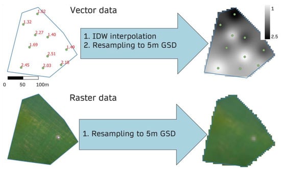
Figure 4.
Data preprocessing process of soil (point vector data) and drone orthomosaic (raster data) data. IDW = inverse distance weighting, GSD = ground sample distance (pixel size on the ground).
The original spatial resolution of the drone orthomosaics was 2–14 cm (Table 2), which means that even small details related to farming operations, such as tractor tracks, were visible. To avoid these external effects, all orthomosaics were resampled (average downsampling) to 5 m GSD. After resampling, we had 797 data points from the smallest field and 1778 data points from the largest field available for analysis.
2.2.6. Statistical Analysis and Machine Learning
The coefficient of variation (CV) was used to measure variability in the field parcels. This is a commonly used and simple metric to measure spatial variability in field parcels [1]. The Pearson correlation coefficient (r) values between all 14 different soil/field-related parameters and drone orthomosaics were calculated in a pixel-wise manner.
To investigate how soil/field-related indicators could explain the within-field variability in the drone orthomosaics, multi-parameter, non-linear models were established using the random forest (RF) algorithm [46]. RF was selected because it has been successfully used in remote sensing studies, mainly because it is relatively insensitive to feature selection and hyper-parameter optimization [47]. In addition, RF measures the importance of input variables to the model. The resampled pixel data were divided so that 75% were used to train and 25% were used to test the models. The test dataset, which was not used in training, was used to evaluate the performance of the models using r and the coefficient of determination (R2) as the evaluation measures. The time range of the drone datasets (2016–2020) was wider than that of the soil measurements (2019–2021). However, the change in the determined soil properties was slow, and the effect of this difference on the analysis was evaluated to be small; therefore, we considered that this generalization was justified.
3. Results
3.1. Correlation Analysis of Single Variables
The Pearson correlation coefficients (r) between preprocessed drone orthomosaics and rasterized soil/field indicators were calculated for all datasets (Figure 5). On fields l1 and l2, the correlations were mainly below 0.55. The highest negative correlation (−0.54) in field l1 was observed between the topsoil biological indicators (A) and both the green and NIR bands collected in July 2020, when spring barley was grown in the field. Positive correlations were relatively low in all cases, yielding, at best, 0.38.
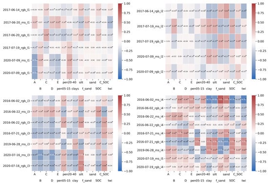
Figure 5.
The correlation coefficients between drone datasets and soil properties for all datasets collected in experimental fields l1, l2, i3, and i4. * indicates that the correlation was significant based on the Wald Test with t-distribution (p < 0.05). A = topsoil biological indicators, B = subsoil macroporosity, C = compacted layers in soil profile, D = topsoil structure, E = subsoil structure, pen05–15 = mean soil penetration resistance in the 5–15 cm layer, and pen20–40 = in the 20–40 cm layer, SOC = soil organic carbon content, C_SOC = clay/soil organic carbon ratio in the 0–20 cm layer.
In field l2, the highest correlations were achieved for the soil texture parameter sand (r = 0.43) and for the topography variable TWI (r = −0.45), with the gRGB dataset collected on 14 June 2017.
The correlations were higher for fields i3 and i4 than for fields l1 and l2 (Figure 5). In field i3, the highest correlation was between the NIR orthomosaic band of July 2020 and soil quality indicators B (macropores in subsoil, r = −0.61) and D (topsoil structure, r = −0.60). The highest positive correlation (r = 0.57) was observed between silt content and the RGB dataset from July 2020.
In field i4, significantly high correlations occurred in many cases, particularly between fine sand and the 2016-06-02_ms dataset (r = 0.81), and between the TWI and the same dataset, which showed a negative correlation (r = −0.81). The same soil properties were relatively highly correlated with drone datasets collected in July 2016 and June 2019. TWI appeared to be negatively correlated with the multispectral dataset, especially during the rainy growing season in 2016, when the crop (pea) was suffering under wet conditions.
3.2. Multi-Parameter Non-Linear Models
In field l1, multi-linear RF models explained 40%–84% (R2 = 0.40–0.84) of the variability in the drone data (Table 4). Typically, when the field had more variability based on the CV, the R2 value was also higher. Especially for the datasets collected in 2017, the topography variable was among the most important indicators that contributed to the models. Furthermore, other soil variables, such as silt content and various soil quality indicators, were ranked among the three most important variables (Table 4).
Table 4.
Coefficient of variation (CV), R2, and r values of random forest models (the highest values of each field is bolded) and the three most important features affecting the model (datasets for RGB or multispectral (MS) cameras in fields l1, l2, i3, and i4). Acronyms of soil indicators as in Table 3.
In field l2, the RF model using the MS dataset collected in July 2017 resulted in R2 = 0.62 (Table 4). Other models yielded lower R2 values. Topography and soil clay content were the most common variables among the three most important predictors that contributed to the models. Based on these results, the R2 values were lower in fields l1 and l2 in years when the crop was grass (2017 and 2020, respectively (Table 2 and Table 4)). This may have been due to the better resilience of grass to variations in soil and growing season weather conditions compared to annual crops.
In field i3, the RF models explained 77–95% (R2 = 0.77–0.95) of the variability in the drone datasets (Table 3). High R2 values (>0.80) were achieved in all datasets collected in 2016 and 2020. In the 2019 dataset, the R2 value was the lowest (0.77), but it was still relatively high. The most important variables that contributed to the models were penetrometer resistance, especially from topsoil (pen05–15), soil quality indicators B (subsoil macroporosity) and D (topsoil structure), and soil silt content (Table 4).
In field i4, R2 varied from 0.32 to 0.90. The RF models were able to relatively effectively explain the variability in all datasets collected during 2016–2019, but in 2020, R2 was lower (R2 0.32). On the other hand, in 2020, the variability in the field was lower than in other years based on the CV measurements (Table 4). The topographic variable (TWI), SOC, penetrometer measurements, and soil biological indicators in the topsoil were the most common variables to occur among the three most important variables.
4. Discussion
4.1. Assessment of the Correlations and Multi-Parameter Models
In this study, we evaluated the relationship between drone image data and soil/field properties, with a focus on how topography and basic soil quality indicators could explain spatial variability in agricultural fields observed from drone orthomosaics. Firstly, we presented pixel-wise linear correlations between drone datasets and soil-related parameters. Secondly, we trained and tested multi-parameter non-linear RF models, where all 14 available soil/field-related indicators were used as features to explain the multispectral (NIR band) and RGB (green band) drone datasets.
The Pearson correlation coefficients between individual indicators and drone datasets were not consistent in the examined fields over the years, i.e., there were no indicators which strongly correlated with all datasets throughout all seasons and years. The fact that spatial variation was not similar across all datasets affected the correlations. We calculated the CVs of drone orthomosaics in the fields and noted that they varied between the four fields; however, they varied even more within the same field when comparing datasets collected in different years and at different times within a growing season. Similarly, the temporal variability in yield maps was found to be greater than their spatial variability, which was especially attributable to the variation in precipitation between years [48]. Indeed, in the present study, one likely reason for the variation in correlations was that the studied crops differed in terms of how they responded to the prevailing weather conditions [49] depending on soil properties and indicators (Appendix A).
Multi-parameter RF models using 14 soil indicators explained the variability in the drone data well (R2 > 0.50), for the most part, when annual crops were grown. The crop-related variation in drone images could also be attributed to aspects other than soil, such as lodging, mistakes in crop sowing and management, pests and diseases of plants, and extreme weather conditions (wetness/dryness) (e.g., [8]). The number of soil sampling points (10–12 per field) was probably too small to capture the field variation as a whole, even though the samples were interpolated to continuous raster maps for entire fields. In datasets where the crop was perennial grass, R2 was generally lower. The reason for this might be that perennial grass stands were already well established and may thereby have had better resilience to variations in soil and weather conditions than annual crops. On the other hand, they may have faced more non-soil-related issues in Nordic conditions, such as winter damage, which may again cause spatial variation in growth and biomass production. The time window to affect the growth of annual crops is shorter than that for perennial crops. In high-latitude conditions, the growing season is especially short and intensive, and therefore annual crops have a low capacity later in the growing season to compensate for losses caused by even temporary weather constraints [50,51].
Our drone data included 15 RGB camera (Green band) and 12 MS camera (NIR band) reflectance orthomosaics, of which 10 were collected simultaneously. The single correlations between RGB and MS orthomosaics and soil indicators from the same dates were generally at similar levels, but in datasets collected on 2 June 2016 in field i4, the MS dataset achieved significantly higher correlations; this was when the crop (pea) was in its early growing stage and did not yet cover much soil, which may explain the result, because the signal from young crops is stronger in the NIR than in the green band. When comparing results from multi-parameter models, the MS datasets yielded higher R2 values in general, but the differences between them were relatively small. This observation is in line with the literature on crop parameter estimation using RGB and NIR bands; typically, NIR bands or indices have shown a stronger connection to crop parameters such as biomass, but RGB data may achieve similar results in remote sensing models using deep learning techniques [52,53].
4.2. Explainability of Individual Topography and Soil Indicators in Study Fields Based on Drone Image Data
We reported the three most important soil/field-related variables that explained the variability in drone images and observed that they varied between fields and imaging times during one year, but also between years. However, based on these findings and those of our correlation analysis, some conclusions about the importance of indicators in studying fields can be drawn.
TWI appeared to be an important variable for explaining the spatial variability in drone images in many experiments. In particular, high correlations occurred in field i4, where TWI was negatively correlated with the multispectral dataset during the rainy growing season of 2016, when the crop (pea) was suffering from wet soil conditions (Figure A2 in Appendix A). This is a logical result, since the NIR band corresponds well to chlorophyll content and reaches low values when vegetation is in distress [54]; this was observed in our study in valleys, where the TWI reached high values but the vegetation was in distress. The correlation was strongest (−0.81) during the early growth stages. In 2019, the correlation was the opposite (positive) when the growing season was dry, and the crop (spring barley) was suffering from dryness on the upper slope and growing well in valleys (Figure 2 and Figure 3). In agreement with our results, Da Silva and Silva [55] also reported strong correlations (correlation coefficients up to 0.95) between maize yield and TWI in Portugal in a three-year period when water was limited. Furthermore, Kumhalova and Matějková [56] achieved correlation coefficients of up to 0.63 between winter wheat yields and TWI in their study fields. In addition, TWI was reported to explain 38%–48% of spatial variability in yield in a wheat field in the USA [57]. Our results confirmed that TWI can also be a significant variable for explaining the spatial variability in agricultural fields in boreal conditions.
Correlations between drone images and soil organic carbon (SOC) content or the clay/SOC ratio were generally not very high in any dataset, but they were among the three most important features in the datasets for “l2” and “i4” when using the multiparameter models. Earlier studies have shown that it is possible to estimate SOC using hyperspectral remote sensing data (e.g., [58]). However, Žížala et al. [25] achieved an R2 value of 0.72 and a root-mean-square error (RMSE) of 0.31% for SOC using multispectral drone data and machine learning. It has been shown on a global scale that SOC and yield have a statistically significant but low correlation [59]. Nonetheless, the variability in SOC in individual parcels and its relation to the remote sensing data of crop-covered fields and their yields require further study.
Soil penetrometer resistance, indicating the soil compactness, appeared to be an important variable for explaining the spatial variability in drone images in many datasets in experimental field i3. Together with the soil quality assessment indicators “subsoil macroporosity” and “topsoil structure”, as well as soil texture (silt content), penetrometer resistance determinations formed the most important features for explaining the variability in that field. The relationship between soil compactness and remote sensing data, especially using drones, has not yet been widely studied [23]. Kulkarni et al. [60] nevertheless reported that the vegetation index (green NDVI) and thickness of the soil hardpan were significantly correlated in their study area.
We utilized a group of soil indicators from different data sources, which can consequently be referred to as multi-source data. Our aim was to utilize these data to explain variations in the reflectance values in drone orthomosaic images. Other studies have used multi-source data, including remote sensing and soil data, to predict yield, as described by Van Klompenburg et al. [17]. For instance, Nevavuori et al. [61] reported that the RMSE of yield estimation accuracy was 15% when data from soil sampling, a soil scanner, elevation maps, and weather stations were added to training data, in addition to drone-based RGB images (R2 = 0.53). Our study supports the findings of earlier studies which state that relationships can be found between remote sensing and soil data but, in addition to the interaction between soil and crops, image data signals are affected by other aspects such as farming practices or crops’ reactions to weather conditions [17,23,25].
4.3. Outlook and Concluding Remarks
There are still many opportunities for further improvements in our knowledge of the relationship between soil indicators and optical image data. Our soil data field sampling was based on 10–12 points per field, which were then interpolated to the whole field so that we had 797–1778 data points available. It should be noted that interpolated soil data include uncertainties, which can impact the results. It would be optimal if soil property determinations included more actual measurement points; therefore, we suggest that the results of image analyses be connected to continuous soil property determinations (e.g., using gamma-ray or soil electromagnetic properties (EM)). Our dataset included a multi-annual time series and varying crops in different growth stages. The crop growth stage was not observed systematically during the drone imaging process. In future studies, it will be important to include the phenological stage of crops in the drone image datasets to increase the comparability of datasets between fields and years. Although drone images were collected close to solar noon in relatively stable illumination conditions and were radiometrically processed in order to provide uniform orthomosaics where the variability in the field was only related to the object itself, varying illumination conditions might have had minor effects on the results [32,62]. Thus, it is important to perform rigorous radiometric processing, which can be supported using accurate, tilt-corrected, drone irradiance measurements [63,64], to obtain the most accurate measurements.
In the future, the importance of developing deeper knowledge of field parcel characteristics needs to be emphasized, as such an understanding has been found to play a key role in farmers’ decision-making, and can even be beneficial in cases of robotics and artificial intelligence [65]. More precise knowledge provided by drones about field characteristics, especially regarding variability and its drivers and manageability, can encourage farmers to perform land-use changes [66,67] and better crop sequencing and to use other measures to boost the transition towards more resilient and sustainable agricultural systems [68]. Information about soil growth conditions and their variability is also relevant when evaluating the financial value of a field. Significant consequences of uncertainty in the valuation of fields have been observed; for instance, this uncertainty has limited land consolidation activities in Finland [69]. Remote sensing data can accurately describe spatial variations in the field, but a large-scale network of on-farm experiments is necessary to achieve a comprehensive understanding of the interaction between crop responses (which differ depending on the species and growing conditions), remote sensing data, and soil/field quality indicators (Video S1).
Supplementary Materials
Video S1: A seminar presentation: “Remote sensing as a data source for crop and soil monitoring”, available at https://www.youtube.com/watch?v=U9sPKzC8d1I&t=137s. Accessed on 24 February 2023.
Author Contributions
Conceptualization, R.N., L.A. (Laura Alakukku), and P.P.-S.; methodology, R.N. and L.A. (Laura Alakukku); software, R.N. and R.A.O.; validation, R.N., H.M. and L.A. (Laura Alakukku); formal analysis, R.N.; investigation, R.N. and L.A. (Laura Alakukku); resources, L.A. (Laura Alakukku), N.-S.K., H.M., R.N. and N.K.; data curation, R.N., N.K., L.A., N.-S.K., H.M., M.Ä. and L.A.; writing—original draft preparation, R.N., L.A. (Laura Alakukku), and H.M.; writing—review and editing, R.N., H.M., E.H., N.K., R.A.O., P.P.-S., N.-S.K., M.Ä., L.A. (Lauri Arkkola), and L.A. (Laura Alakukku); visualization, R.N.; supervision, E.H. and L.A. (Laura Alakukku); project administration, E.H. and L.A. (Laura Alakukku); funding acquisition, E.H., L.A. (Laura Alakukku), P.P.-S. and R.N. All authors have read and agreed to the published version of the manuscript.
Funding
This research was funded by Optimising Agricultural Land Use to Mitigate Climate Change (OPAL-Life, LIFE14 CCM/FI/000254; this paper reflects only the authors’ views, and the EASME/Commission is not responsible for any use that may be made of the information it contains); by the Ministry of Agriculture and Forestry in Finland via the MAKERA project “Remote Sensing Methods for Field Quality Assessment and Scoring—Towards Sustainable Field Reform (PELTOPISTE)”, grant no. 469/03.01.02/2019; and by the National Land Survey of Finland and the University of Helsinki.
Data Availability Statement
Data sharing is not applicable to this article.
Acknowledgments
We would like to thank the farmers who allowed us to carry out measurements in their fields. Additionally, we would like to thank Ari Rajala and Jaana Sorvali from the Natural Resources Institute Finland (Luke), Teemu Hakala and Mika Karjalainen from the National Land Survey of Finland, and Jaakko Haarala from the University of Helsinki for their support during the project.
Conflicts of Interest
The authors declare no conflict of interest. The funders had no role in the design of the study; in the collection, analyses, or interpretation of the data; in the writing of the manuscript; or in the decision to publish the results.
Appendix A

Figure A1.
Monthly precipitation, provided by the Finnish meteorological Institute (FMI), from the nearest weather station to research fields l1 and l2 (Oulusalo, Pellonpää). Data were visualized from the main growing season (April–September) during the years of drone data collection (2017 and 2020).


Figure A2.
Monthly precipitation, provided by the Finnish meteorological Institute (FMI), from the nearest weather station to research fields i3 and i4 (Siuntio Sjundby). Data were visualized from the main growing season (April–September) during the years of drone data collection (2016, 2019, and 2020).

References
- Leroux, C.; Tisseyre, B. How to Measure and Report Within-Field Variability: A Review of Common Indicators and Their Sensitivity. Precis. Agric. 2019, 20, 562–590. [Google Scholar] [CrossRef]
- Lark, R.; Catt, J.; Stafford, J. Towards the Explanation of Within-Field Variability of Yield of Winter Barley: Soil Series Differences. J. Agric. Sci. 1998, 131, 409–416. [Google Scholar] [CrossRef]
- Raun, W.R.; Solie, J.B.; Stone, M.L. Independence of Yield Potential and Crop Nitrogen Response. Precis. Agric. 2011, 12, 508–518. [Google Scholar] [CrossRef]
- Keller, T.; Sutter, J.A.; Nissen, K.; Rydberg, T. Using Field Measurement of Saturated Soil Hydraulic Conductivity to Detect Low-Yielding Zones in Three Swedish Fields. Soil Tillage Res. 2012, 124, 68–77. [Google Scholar] [CrossRef]
- Diaz-Gonzalez, F.A.; Vuelvas, J.; Correa, C.A.; Vallejo, V.E.; Patino, D. Machine Learning and Remote Sensing Techniques Applied to Estimate Soil Indicators–Review. Ecol. Indic. 2022, 135, 108517. [Google Scholar] [CrossRef]
- Karlen, D.L.; Mausbach, M.; Doran, J.W.; Cline, R.; Harris, R.; Schuman, G. Soil Quality: A Concept, Definition, and Framework for Evaluation (a Guest Editorial). Soil Sci. Soc. Am. J. 1997, 61, 4–10. [Google Scholar] [CrossRef]
- Nykänen, A.; Jauhiainen, L.; Kemppainen, J.; Lindström, K. Field-Scale Spatial Variation in Yields and Nitrogen Fixation of Clover-Grass Leys and in Soil Nutrients. Agric. Food Sci. 2008, 17, 376–393. [Google Scholar] [CrossRef]
- Hakojärvi, M.; Hautala, M.; Ristolainen, A.; Alakukku, L. Yield Variation of Spring Cereals in Relation to Selected Soil Physical Properties on Three Clay Soil Fields. Eur. J. Agron. 2013, 49, 1–11. [Google Scholar] [CrossRef]
- Juhos, K.; Szabó, S.; Ladányi, M. Explore the Influence of Soil Quality on Crop Yield Using Statistically-Derived Pedological Indicators. Ecol. Indic. 2016, 63, 366–373. [Google Scholar] [CrossRef]
- Lipiec, J.; Usowicz, B. Spatial Relationships among Cereal Yields and Selected Soil Physical and Chemical Properties. Sci. Total Environ. 2018, 633, 1579–1590. [Google Scholar] [CrossRef]
- Weiss, M.; Jacob, F.; Duveiller, G. Remote Sensing for Agricultural Applications: A Meta-Review. Remote Sens. Environ. 2020, 236, 111402. [Google Scholar] [CrossRef]
- Berni, J.A.; Zarco-Tejada, P.J.; Suárez, L.; Fereres, E. Thermal and Narrowband Multispectral Remote Sensing for Vegetation Monitoring from an Unmanned Aerial Vehicle. IEEE Trans. Geosci. Remote Sens. 2009, 47, 722–738. [Google Scholar] [CrossRef]
- Wang, T.; Liu, Y.; Wang, M.; Fan, Q.; Tian, H.; Qiao, X.; Li, Y. Applications of UAS in Crop Biomass Monitoring: A Review. Front. Plant Sci. 2021, 12, 616689. [Google Scholar] [CrossRef]
- Geipel, J.; Link, J.; Wirwahn, J.A.; Claupein, W. A Programmable Aerial Multispectral Camera System for In-Season Crop Biomass and Nitrogen Content Estimation. Agriculture 2016, 6, 4. [Google Scholar] [CrossRef]
- Alves Oliveira, R.; Marcato Junior, J.; Soares Costa, C.; Näsi, R.; Koivumäki, N.; Niemeläinen, O.; Kaivosoja, J.; Nyholm, L.; Pistori, H.; Honkavaara, E. Silage Grass Sward Nitrogen Concentration and Dry Matter Yield Estimation Using Deep Regression and RGB Images Captured by UAV. Agronomy 2022, 12, 1352. [Google Scholar] [CrossRef]
- Gopp, N.; Savenkov, O. Relationships between the NDVI, Yield of Spring Wheat, and Properties of the Plow Horizon of Eluviated Clay-Illuvial Chernozems and Dark Gray Soils. Eurasian Soil Sci. 2019, 52, 339–347. [Google Scholar] [CrossRef]
- Van Klompenburg, T.; Kassahun, A.; Catal, C. Crop Yield Prediction Using Machine Learning: A Systematic Literature Review. Comput. Electron. Agric. 2020, 177, 105709. [Google Scholar] [CrossRef]
- Nevavuori, P.; Narra, N.; Lipping, T. Crop Yield Prediction with Deep Convolutional Neural Networks. Comput. Electron. Agric. 2019, 163, 104859. [Google Scholar] [CrossRef]
- Mohidem, N.A.; Che’Ya, N.N.; Juraimi, A.S.; Fazlil Ilahi, W.F.; Mohd Roslim, M.H.; Sulaiman, N.; Saberioon, M.; Mohd Noor, N. How Can Unmanned Aerial Vehicles Be Used for Detecting Weeds in Agricultural Fields? Agriculture 2021, 11, 1004. [Google Scholar] [CrossRef]
- Peña, J.M.; Torres-Sánchez, J.; de Castro, A.I.; Kelly, M.; López-Granados, F. Weed Mapping in Early-Season Maize Fields Using Object-Based Analysis of Unmanned Aerial Vehicle (UAV) Images. PLoS ONE 2013, 8, e77151. [Google Scholar] [CrossRef]
- Zarco-Tejada, P.J.; González-Dugo, V.; Berni, J.A. Fluorescence, Temperature and Narrow-Band Indices Acquired from a UAV Platform for Water Stress Detection Using a Micro-Hyperspectral Imager and a Thermal Camera. Remote Sens. Environ. 2012, 117, 322–337. [Google Scholar] [CrossRef]
- Manfreda, S.; McCabe, M.F.; Miller, P.E.; Lucas, R.; Pajuelo Madrigal, V.; Mallinis, G.; Ben Dor, E.; Helman, D.; Estes, L.; Ciraolo, G. On the Use of Unmanned Aerial Systems for Environmental Monitoring. Remote Sens. 2018, 10, 641. [Google Scholar] [CrossRef]
- Khanal, S.; Kc, K.; Fulton, J.P.; Shearer, S.; Ozkan, E. Remote Sensing in Agriculture—Accomplishments, Limitations, and Opportunities. Remote Sens. 2020, 12, 3783. [Google Scholar] [CrossRef]
- Hu, J.; Peng, J.; Zhou, Y.; Xu, D.; Zhao, R.; Jiang, Q.; Fu, T.; Wang, F.; Shi, Z. Quantitative Estimation of Soil Salinity Using UAV-Borne Hyperspectral and Satellite Multispectral Images. Remote Sens. 2019, 11, 736. [Google Scholar] [CrossRef]
- Žížala, D.; Minařík, R.; Zádorová, T. Soil Organic Carbon Mapping Using Multispectral Remote Sensing Data: Prediction Ability of Data with Different Spatial and Spectral Resolutions. Remote Sens. 2019, 11, 2947. [Google Scholar] [CrossRef]
- Aldana-Jague, E.; Heckrath, G.; Macdonald, A.; van Wesemael, B.; Van Oost, K. UAS-Based Soil Carbon Mapping Using VIS-NIR (480–1000 Nm) Multi-Spectral Imaging: Potential and Limitations. Geoderma 2016, 275, 55–66. [Google Scholar] [CrossRef]
- Khanal, S.; Fulton, J.; Klopfenstein, A.; Douridas, N.; Shearer, S. Integration of High Resolution Remotely Sensed Data and Machine Learning Techniques for Spatial Prediction of Soil Properties and Corn Yield. Comput. Electron. Agric. 2018, 153, 213–225. [Google Scholar] [CrossRef]
- ProAgria 2022. Peltomaan Laatutesti. 2022. Available online: https://www.proagria.fi/uploads/archive/attachment/peltomaan_laatutesti_havaintojen_ja_mittausten_teko-ohjeet.pdf (accessed on 23 February 2023).
- Finnish Meteorological Institute. Suomen Ilmastovyöhykkeet. 2023. Available online: https://www.ilmatieteenlaitos.fi/suomen-ilmastovyohykkeet (accessed on 23 February 2023). (In Finnish).
- Finnish Meteorological Institute. Valitse Oikea Kasvi Oikealle Kasvuvyöhykkeelle. 2023. Available online: https://www.ilmatieteenlaitos.fi/kasvuvyohykkeet (accessed on 23 February 2023). (In Finnish).
- Mäkynen, J.; Holmlund, C.; Saari, H.; Ojala, K.; Antila, T. Unmanned Aerial Vehicle (UAV) Operated Megapixel Spectral Camera; SPIE: Bellingham, WA, USA, 2011; Volume 8186, pp. 295–303. [Google Scholar]
- Honkavaara, E.; Saari, H.; Kaivosoja, J.; Pölönen, I.; Hakala, T.; Litkey, P.; Mäkynen, J.; Pesonen, L. Processing and Assessment of Spectrometric, Stereoscopic Imagery Collected Using a Lightweight UAV Spectral Camera for Precision Agriculture. Remote Sens. 2013, 5, 5006–5039. [Google Scholar] [CrossRef]
- Hakala, T.; Markelin, L.; Honkavaara, E.; Scott, B.; Theocharous, T.; Nevalainen, O.; Näsi, R.; Suomalainen, J.; Viljanen, N.; Greenwell, C. Direct Reflectance Measurements from Drones: Sensor Absolute Radiometric Calibration and System Tests for Forest Reflectance Characterization. Sensors 2018, 18, 1417. [Google Scholar] [CrossRef]
- Viljanen, N.; Honkavaara, E.; Näsi, R.; Hakala, T.; Niemeläinen, O.; Kaivosoja, J. A Novel Machine Learning Method for Estimating Biomass of Grass Swards Using a Photogrammetric Canopy Height Model, Images and Vegetation Indices Captured by a Drone. Agriculture 2018, 8, 70. [Google Scholar] [CrossRef]
- Wu, Y.; Lim, J.; Yang, M.-H. Online Object Tracking: A Benchmark. In Proceedings of the IEEE Conference on Computer Vision and Pattern Recognition, New York, NY, USA, 23–28 June 2013; pp. 2411–2418. [Google Scholar]
- Näsi, R.; Honkavaara, E.; Lyytikäinen-Saarenmaa, P.; Blomqvist, M.; Litkey, P.; Hakala, T.; Viljanen, N.; Kantola, T.; Tanhuanpää, T.; Holopainen, M. Using UAV-Based Photogrammetry and Hyperspectral Imaging for Mapping Bark Beetle Damage at Tree-Level. Remote Sens. 2015, 7, 15467–15493. [Google Scholar] [CrossRef]
- Holman, F.H.; Riche, A.B.; Castle, M.; Wooster, M.J.; Hawkesford, M.J. Radiometric Calibration of ‘Commercial off the Shelf’Cameras for UAV-Based High-Resolution Temporal Crop Phenotyping of Reflectance and NDVI. Remote Sens. 2019, 11, 1657. [Google Scholar] [CrossRef]
- Burggraaff, O.; Schmidt, N.; Zamorano, J.; Pauly, K.; Pascual, S.; Tapia, C.; Spyrakos, E.; Snik, F. Standardized Spectral and Radiometric Calibration of Consumer Cameras. Opt. Express 2019, 27, 19075–19101. [Google Scholar] [CrossRef] [PubMed]
- Mattivi, P.; Franci, F.; Lambertini, A.; Bitelli, G. TWI Computation: A Comparison of Different Open Source GISs. Open Geospat. Data Softw. Stand. 2019, 4, 6. [Google Scholar] [CrossRef]
- Alakukku, L. Properties of Compacted Fine-Textured Soils as Affected by Crop Rotation and Reduced Tillage. Soil Tillage Res. 1998, 47, 83–89. [Google Scholar] [CrossRef]
- Pietola, L. Effect of Soil Compactness on the Growth and Quality of Carrot. Agric. Food Sci. 1995, 4, 139–237. [Google Scholar] [CrossRef]
- Li, J.; Heap, A.D. Spatial Interpolation Methods Applied in the Environmental Sciences: A Review. Environ. Model. Softw. 2014, 53, 173–189. [Google Scholar] [CrossRef]
- Shepard, D. A Two-Dimensional Interpolation Function for Irregularly-Spaced Data. In Proceedings of the 1968 23rd ACM National Conference, New York, NY, USA, 27–29 August 1968; pp. 517–524. [Google Scholar]
- Bărbulescu, A.; Șerban, C.; Indrecan, M.-L. Computing the Beta Parameter in IDW Interpolation by Using a Genetic Algorithm. Water 2021, 13, 863. [Google Scholar] [CrossRef]
- Radočaj, D.; Jug, I.; Vukadinović, V.; Jurišić, M.; Gašparović, M. The Effect of Soil Sampling Density and Spatial Autocorrelation on Interpolation Accuracy of Chemical Soil Properties in Arable Cropland. Agronomy 2021, 11, 2430. [Google Scholar] [CrossRef]
- Breiman, L. Random Forests. Mach. Learn. 2001, 45, 5–32. [Google Scholar] [CrossRef]
- Belgiu, M.; Drăguţ, L. Random Forest in Remote Sensing: A Review of Applications and Future Directions. ISPRS J. Photogramm. Remote Sens. 2016, 114, 24–31. [Google Scholar] [CrossRef]
- Maestrini, B.; Basso, B. Drivers of Within-Field Spatial and Temporal Variability of Crop Yield across the US Midwest. Sci. Rep. 2018, 8, 14833. [Google Scholar] [CrossRef] [PubMed]
- Peltonen-Sainio, P.; Jauhiainen, L.; Hakala, K. Crop Responses to Temperature and Precipitation According to Long-Term Multi-Location Trials at High-Latitude Conditions. J. Agric. Sci. 2011, 149, 49–62. [Google Scholar] [CrossRef]
- Peltonen-Sainio, P.; Venäläinen, A.; Mäkelä, H.M.; Pirinen, P.; Laapas, M.; Jauhiainen, L.; Kaseva, J.; Ojanen, H.; Korhonen, P.; Huusela-Veistola, E. Harmfulness of Weather Events and the Adaptive Capacity of Farmers at High Latitudes of Europe. Clim. Res. 2016, 67, 221–240. [Google Scholar] [CrossRef]
- Peltonen-Sainio, P.; Jauhiainen, L.; Trnka, M.; Olesen, J.E.; Calanca, P.; Eckersten, H.; Eitzinger, J.; Gobin, A.; Kersebaum, K.C.; Kozyra, J. Coincidence of Variation in Yield and Climate in Europe. Agric. Ecosyst. Environ. 2010, 139, 483–489. [Google Scholar] [CrossRef]
- Poley, L.G.; McDermid, G.J. A Systematic Review of the Factors Influencing the Estimation of Vegetation Aboveground Biomass Using Unmanned Aerial Systems. Remote Sens. 2020, 12, 1052. [Google Scholar] [CrossRef]
- Karila, K.; Alves Oliveira, R.; Ek, J.; Kaivosoja, J.; Koivumäki, N.; Korhonen, P.; Niemeläinen, O.; Nyholm, L.; Näsi, R.; Pölönen, I. Estimating Grass Sward Quality and Quantity Parameters Using Drone Remote Sensing with Deep Neural Networks. Remote Sens. 2022, 14, 2692. [Google Scholar] [CrossRef]
- Gitelson, A.A.; Viña, A.; Ciganda, V.; Rundquist, D.C.; Arkebauer, T.J. Remote Estimation of Canopy Chlorophyll Content in Crops. Geophys. Res. Lett. 2005, 32. [Google Scholar] [CrossRef]
- Da Silva, J.M.; Silva, L.L. Evaluation of the Relationship between Maize Yield Spatial and Temporal Variability and Different Topographic Attributes. Biosyst. Eng. 2008, 101, 183–190. [Google Scholar] [CrossRef]
- Kumhalova, J.; Matějková, Š. Yield Variability Prediction by Remote Sensing Sensors with Different Spatial Resolution. Int. Agrophys. 2017, 31, 195. [Google Scholar] [CrossRef]
- Green, T.R.; Erskine, R.H. Measurement, Scaling, and Topographic Analyses of Spatial Crop Yield and Soil Water Content. Hydrol. Process. 2004, 18, 1447–1465. [Google Scholar] [CrossRef]
- Gomez, C.; Rossel, R.A.V.; McBratney, A.B. Soil Organic Carbon Prediction by Hyperspectral Remote Sensing and Field Vis-NIR Spectroscopy: An Australian Case Study. Geoderma 2008, 146, 403–411. [Google Scholar] [CrossRef]
- Oldfield, E.E.; Bradford, M.A.; Wood, S.A. Global Meta-Analysis of the Relationship between Soil Organic Matter and Crop Yields. Soil 2019, 5, 15–32. [Google Scholar] [CrossRef]
- Kulkarni, S.; Bajwa, S.; Huitink, G. Investigation of the Effects of Soil Compaction in Cotton. Trans. ASABE 2010, 53, 667–674. [Google Scholar] [CrossRef]
- Nevavuori, P.; Narra, N.; Linna, P.; Lipping, T. Assessment of Crop Yield Prediction Capabilities of CNN Using Multisource Data. In New Developments and Environmental Applications of Drones; Springer: Berlin/Heidelberg, Germany, 2022; pp. 173–186. [Google Scholar]
- Änäkkälä, M.; Lajunen, A.; Hakojärvi, M.; Alakukku, L. Evaluation of the Influence of Field Conditions on Aerial Multispectral Images and Vegetation Indices. Remote Sens. 2022, 14, 4792. [Google Scholar] [CrossRef]
- Suomalainen, J.; Hakala, T.; Alves de Oliveira, R.; Markelin, L.; Viljanen, N.; Näsi, R.; Honkavaara, E. A Novel Tilt Correction Technique for Irradiance Sensors and Spectrometers On-Board Unmanned Aerial Vehicles. Remote Sens. 2018, 10, 2068. [Google Scholar] [CrossRef]
- Suomalainen, J.; Oliveira, R.A.; Hakala, T.; Koivumäki, N.; Markelin, L.; Näsi, R.; Honkavaara, E. Tilt correction of onboard drone irradiance measurements–evaluation of hyperspectral methods. Int. Arch. Photogramm. Remote Sens. Spat. Inf. Sci. 2022, 43, 67–72. [Google Scholar] [CrossRef]
- Saiz-Rubio, V.; Rovira-Más, F. From Smart Farming towards Agriculture 5.0: A Review on Crop Data Management. Agronomy 2020, 10, 207. [Google Scholar] [CrossRef]
- Peltonen-Sainio, P.; Jauhiainen, L.; Laurila, H.; Sorvali, J.; Honkavaara, E.; Wittke, S.; Karjalainen, M.; Puttonen, E. Land Use Optimization Tool for Sustainable Intensification of High-Latitude Agricultural Systems. Land Use Policy 2019, 88, 104104. [Google Scholar] [CrossRef]
- Trevisan, R.; Bullock, D.; Martin, N. Spatial Variability of Crop Responses to Agronomic Inputs in On-Farm Precision Experimentation. Precis. Agric. 2021, 22, 342–363. [Google Scholar] [CrossRef]
- Peltonen-Sainio, P.; Jauhiainen, L. Risk of Low Productivity Is Dependent on Farm Characteristics: How to Turn Poor Performance into an Advantage. Sustainability 2019, 11, 5504. [Google Scholar] [CrossRef]
- Rikkonen, P.; Lahnamäki-Kivelä, S.; Leppänen, J.; Hänninen, H. Pellonomistajat Ja Maatalouden Tilusrakenteen Kehittäminen 2020-Luvulla. 2022. Available online: https://jukuri.luke.fi/handle/10024/551740 (accessed on 23 February 2023). (In Finnish).


Disclaimer/Publisher’s Note: The statements, opinions and data contained in all publications are solely those of the individual author(s) and contributor(s) and not of MDPI and/or the editor(s). MDPI and/or the editor(s) disclaim responsibility for any injury to people or property resulting from any ideas, methods, instructions or products referred to in the content. |
© 2023 by the authors. Licensee MDPI, Basel, Switzerland. This article is an open access article distributed under the terms and conditions of the Creative Commons Attribution (CC BY) license (https://creativecommons.org/licenses/by/4.0/).