Abstract
The efficiency of agricultural practices depends on the timing of their execution. Environmental conditions, such as rainfall, and crop-related traits, such as plant phenology, determine the success of practices such as irrigation. Moreover, plant phenology, the seasonal timing of biological events (e.g., cotyledon emergence), is strongly influenced by genetic, environmental, and management conditions. Therefore, assessing the timing the of crops’ phenological events and their spatiotemporal variability can improve decision making, allowing the thorough planning and timely execution of agricultural operations. Conventional techniques for crop phenology monitoring, such as field observations, can be prone to error, labour-intensive, and inefficient, particularly for crops with rapid growth and not very defined phenophases, such as vegetable crops. Thus, developing an accurate phenology monitoring system for vegetable crops is an important step towards sustainable practices. This paper evaluates the ability of computer vision (CV) techniques coupled with deep learning (DL) (CV_DL) as tools for the dynamic phenological classification of multiple vegetable crops at the subfield level, i.e., within the plot. Three DL models from the Single Shot Multibox Detector (SSD) architecture (SSD Inception v2, SSD MobileNet v2, and SSD ResNet 50) and one from You Only Look Once (YOLO) architecture (YOLO v4) were benchmarked through a custom dataset containing images of eight vegetable crops between emergence and harvest. The proposed benchmark includes the individual pairing of each model with the images of each crop. On average, YOLO v4 performed better than the SSD models, reaching an F1-Score of 85.5%, a mean average precision of 79.9%, and a balanced accuracy of 87.0%. In addition, YOLO v4 was tested with all available data approaching a real mixed cropping system. Hence, the same model can classify multiple vegetable crops across the growing season, allowing the accurate mapping of phenological dynamics. This study is the first to evaluate the potential of CV_DL for vegetable crops’ phenological research, a pivotal step towards automating decision support systems for precision horticulture.
1. Introduction
Plant phenology comprises the seasonal timing of biological events (e.g., cotyledon emergence) and the causes of their timing concerning biotic and abiotic interactions (agricultural practices included) [1,2].
The timing of crops’ phenological phases (phenophases) provides valuable information for monitoring and simulating plant growth and development. Therefore, it allows the thorough planning and timely execution of agricultural practices, which are usually carried out according to specific phenophases (e.g., timing of irrigation and harvest), leading to higher and more stable crop yields, sustainable practices, and improved food quality [3,4].
Field observation, crop growth models and remote sensing approaches are the most common methods for phenology monitoring. Field observation involves in situ plant assessment and the manual recording of phenophases (e.g., leaf unfolding). This observational approach is laborious and prone to error due to the large spatiotemporal variability of phenophases among plants [5,6]. Consequently, an increased sampling density is needed to adequately represent crop phenology at the field scale. Although crop growth models can simulate the timing of the phenophases of a particular genotype (individual), they cannot transpose the simulation to different spatial scales, as the heterogeneities in climate and management conditions are neglected [7,8,9]. Moreover, near-surface remote sensing techniques, such as digital repeat photography [10,11], and satellite remote sensing linked with vegetation indices (e.g., leaf area index) provide valuable data about phenology dynamics at a regional scale [12]. However, the ability of these methods to monitor phenology at the field or subfield scale is limited, especially in crops with hardly perceivable phenophase transitions such as vegetable crops [13].
Vegetable crops (see https://www.ishs.org/defining-horticulture, last accessed: 18 September 2022), are characterised by rapid growth, which leads to not very defined phenophases. Since most of them are fresh food, the timing of sensitive phenological events, such as cotyledon emergence, is of economic and technical concern to establish accurate practices, such as weed removal [14,15]. Therefore, it is important to set alternative methods suitable for reliably and operationally assessing vegetable crops’ phenophases to support precision horticulture (PH) production systems.
The dynamics of crop phenophases result from a set of structural, physiological, and performance-related phenotypic traits that characterise the given genotype and its interactions with the environment [16]. Computer vision (CV) has attracted growing interest in the agricultural domain as it comprises techniques that allow systems to automatically collect images and extract valuable information from them towards accurate and efficient practices [17]. Usually, CV-based systems include an image acquisition phase and image analysis techniques that can distinguish the regions of interest to be detected and classified (e.g., whole plant, leaves) [18,19]. Among the plethora of image analysis techniques already developed, the one that best performs object detection in agriculture (e.g., disease detection [20], crop and weed detection [21], and fruit detection [22]) is deep learning (DL) [23]. DL is based on machine learning and has led to breakthroughs in image analysis, given its ability to automatically extract features from unstructured data [24]. In particular, convolutional neural networks (CNNs) are being tested for various tasks to support PH production systems, including phenology monitoring [25,26]. Thereby, it is hypothesised that high-throughput plant phenotyping techniques [27] based on CV coupled with DL (CV_DL) can assess the spatiotemporal dynamics of crop traits related to its phenophases in the context of PH [28].
Nevertheless, applications of CV and DL in phenology monitoring are mostly focused on arable crops (e.g., rice, barley, maize) [29,30,31,32], orchards [33,34], and forest trees [35,36,37] with limited studies into vegetable crops. Additionally, the developed models are crop-specific and tend to be based on well-defined phenophases, such as flowering [13,33,35], neglecting the spatiotemporal phenology dynamics. Vegetables usually grow as annual crops and are harvested during the vegetative phase. Thus, the phenotypic traits for phenological identification are restricted to leaves (e.g., number, size, and colour). Furthermore, considering that vegetable crops are often sown as mixed cropping, and the morphological traits of leaves are very similar between plants, especially in the early growth stages, it is difficult to identify the specific phenotypic traits in order to classify the phenophases of the corresponding plant (crops and weeds included) [38,39,40].
This study primarily aims to develop an automatic approach for the dynamic phenological classification of vegetable crops using CV_DL techniques. Four state-of-the-art DL models were tested through a custom dataset that consists of RGB and greyscale annotated images corresponding to the main phenophases of eight vegetable crops between emergence and harvest. Thus, this work contributes to the state-of-the-art introducing a vegetable crop classification system that can identify multiple crops considering phenology dynamics throughout the growing season at the subfield scale.
2. Materials and Methods
2.1. Dataset Acquisition and Processing
Eight vegetable crops were selected to build a varied dataset of phenophases (Table 1), taking into account the length of the growing season, the intensity of agricultural practices (mainly weed removal), and the resistance to pests and diseases.

Table 1.
Vegetable crops selected for the phenophase image dataset construction.
Each crop was manually sown in a section of a 4.5 m2 plot at a greenhouse in Vairão, Vila do Conde, Portugal, according to the recommended sowing density. Weeds were manually removed at an early growth stage (less than four unfolded leaves), and plants were irrigated twice a day. Image acquisition occurred before the weed removal operation.
Images in the RGB colour space were acquired between March and July 2021 by a smartphone (Huawei Mate 10 Lite, 16 MP resolution in Pro Mode) in different view angles and sunlight conditions, both procedures increasing the data representativeness.
Depending on the crop, one or several growing seasons occurred during the image acquisition operation, and images were collected covering the main vegetative phenophases of the crops studied. The classification of the phenophases of each crop was based on the BBCH-scale [41]. In total, there were collected 4123 images with a resolution of 3456 × 4608 px each. Table 2 depicts the dataset: the number of images and plants of each crop and phenophase, accordingly.

Table 2.
Number of images acquired for each crop and the corresponding number of plants for each phenophase defined.
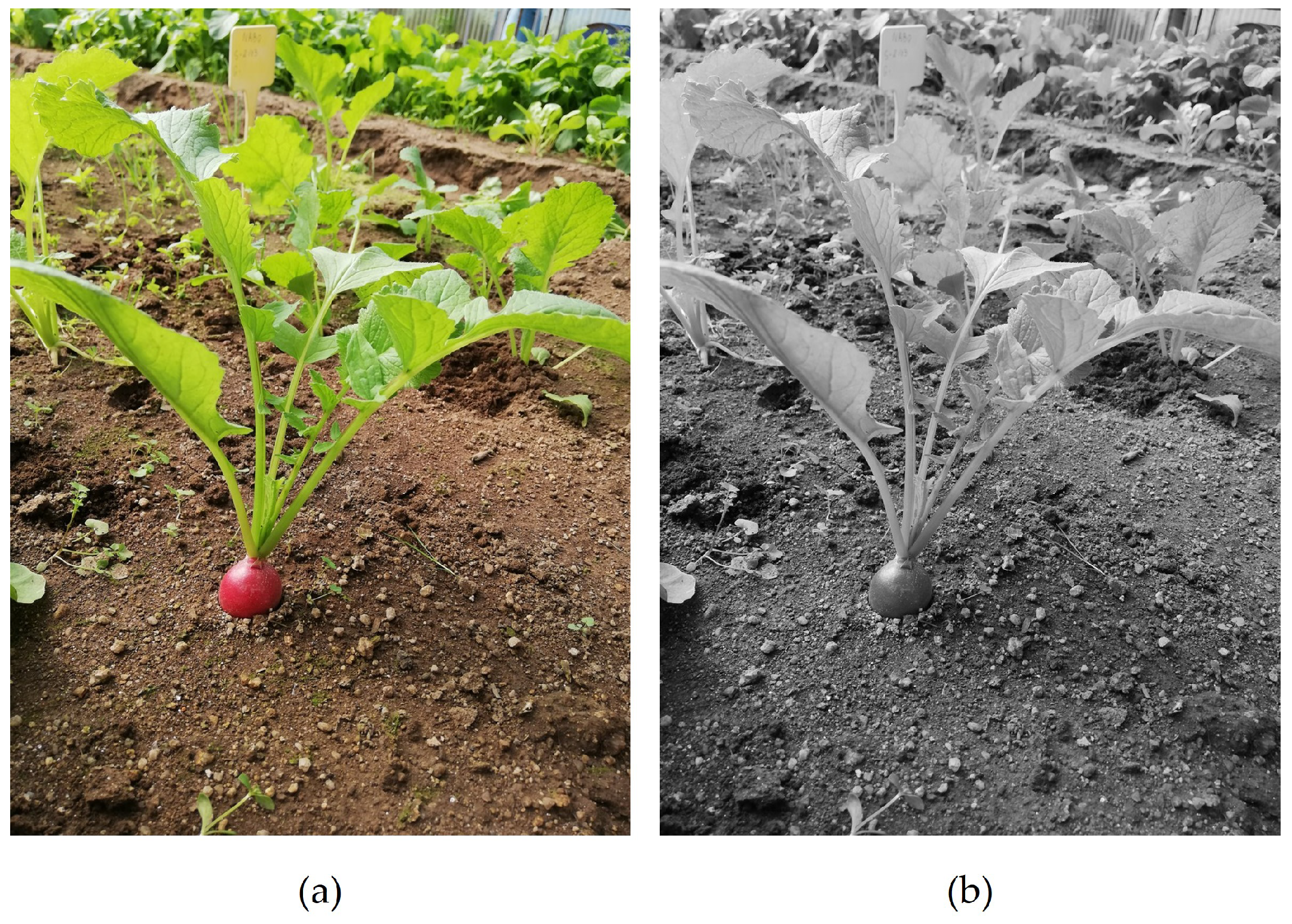
All images were rescaled four times to a resolution of 864 × 1152 px, improving the processing operations. To evaluate the versatility of the DL models studied, the RGB images were also transformed into greyscale using OpenCV (see https://opencv.org, last accessed: 12 September 2022) library. With this transformation, the complexity and the bias are reduced, as the model is not influenced by the colour in the images, while it is forced to learn features that are not specific to colour, improving the generalisation ability. By applying the luminosity method, it is possible to assign a weighted average of the colour components to each RGB channel (see https://docs.opencv.org/4.x/de/d25/imgproc_color_conversions.html, last accessed: 12 September 2022) (Equation (1)). An example of this transformation is presented in Figure 1.

Figure 1.
Radish image acquired in RGB colour space (a) and after greyscale transformation (b).
Since the training and evaluation of DL models involves supervised learning, the images need to be annotated. Following the BBCH-scale [41] and the phenophases defined for each crop (Table 2), images were manually annotated using the open source annotation tool CVAT (see https://www.cvat.ai/, last accessed: 18 September 2022), indicating by rectangular bounding boxes the position and phenophase of each plant. After annotation, the images and the corresponding annotations were exported under the Pascal VOC [42] and YOLO formats [43] to train the SSD and YOLO models, respectively. All annotated images (RGB and greyscale) are publicly available at the open access digital repository Zenodo (see https://doi.org/10.5281/zenodo.7433286, last accessed: 5 November 2022) [44].
2.2. Deep Learning Approach
2.2.1. Object Detection Models
Object detection models are specialised DL models designed to detect the position and size of objects in an image. There are different kinds of DL architectures to detect objects, but the most common ones in the state of the art are based on single-shot CNN, such as SSD and YOLO.
SSD was first introduced by Liu et al. [45]. This architecture comprises three main components: the feature extractor, the classifier, and the regressor. The feature extractor is a CNN frequently designated as the backbone and can be any classification network. Three state-of-the-art backbones were selected for this work: Inception v2, MobileNet v2, and ResNet50. These networks were selected due to the good results obtained in previous works on object detection in agriculture [46,47]. The image was then split into different sizes and positioned windows during the image processing stage. The classifier element will predict the object in each window, and the regressor will adjust the window (also called the bounding box) to the object’s position and size. Combining the three elements (feature extractor, classifier and regressor) leads to an object detection model.
Inception V2, MobileNet v2, and ResNet 50 are three state-of-the-art CNNs. Inception v2 [48] is an improvement of GoogLeNet, also named Inception v1 [49]. This network is made of inception modules and batch normalisation layers. MobileNet v2 is a CNN classifier designed for mobile and embedded applications [50]. In this network, the authors replaced the full convolutional operators with a factorised version that splits the convolution into two layers. The first layer is a lightweight filter, while the other layer is a point-wise operator which creates new features. As such, MobileNet v2 reduced the number of trainable parameters and training complexity. To improve the results of VGG DL models, He et al. [51] studied residual neural networks. ResNet is based on plain architectures with shortcuts for residual learning. This strategy reduced the number of trainable parameters and the training complexity against VGG. ResNet models allow depths between 18 and 152 layers, but ResNet 50 is the most common in the literature.
You Only Look Once (YOLO) is also a well-known single-shot detector, serving most of the time as a reference object detector. YOLO v4 is the fourth generation of YOLO models [52], which delivered multiple features to the original YOLO version, improving the model’s performance and keeping the inference speed. YOLO uses a backbone of DarkNet (see https://pjreddie.com/darknet/, last accessed: 14 October 2022). Among the selected models, YOLO v4 aims to be the one which provides the best balance between accuracy and inference speed. Therefore, this study covers the most current object detection architectures in the literature, especially concerning DL applications in agriculture.
2.2.2. Models Training
For training purposes, the dataset was divided into three sets: training, validation, and test sets. Table 3 depicts the number of images and plants of each crop and phenophase, respectively, assigned for each set (considering only RGB images). The dataset split rate was determined by considering the corresponding number of images and plants in each phenophase.

Table 3.
Dataset split of each crop and phenophase images and plants for the training and evaluation of deep learning models (considering only RGB images).
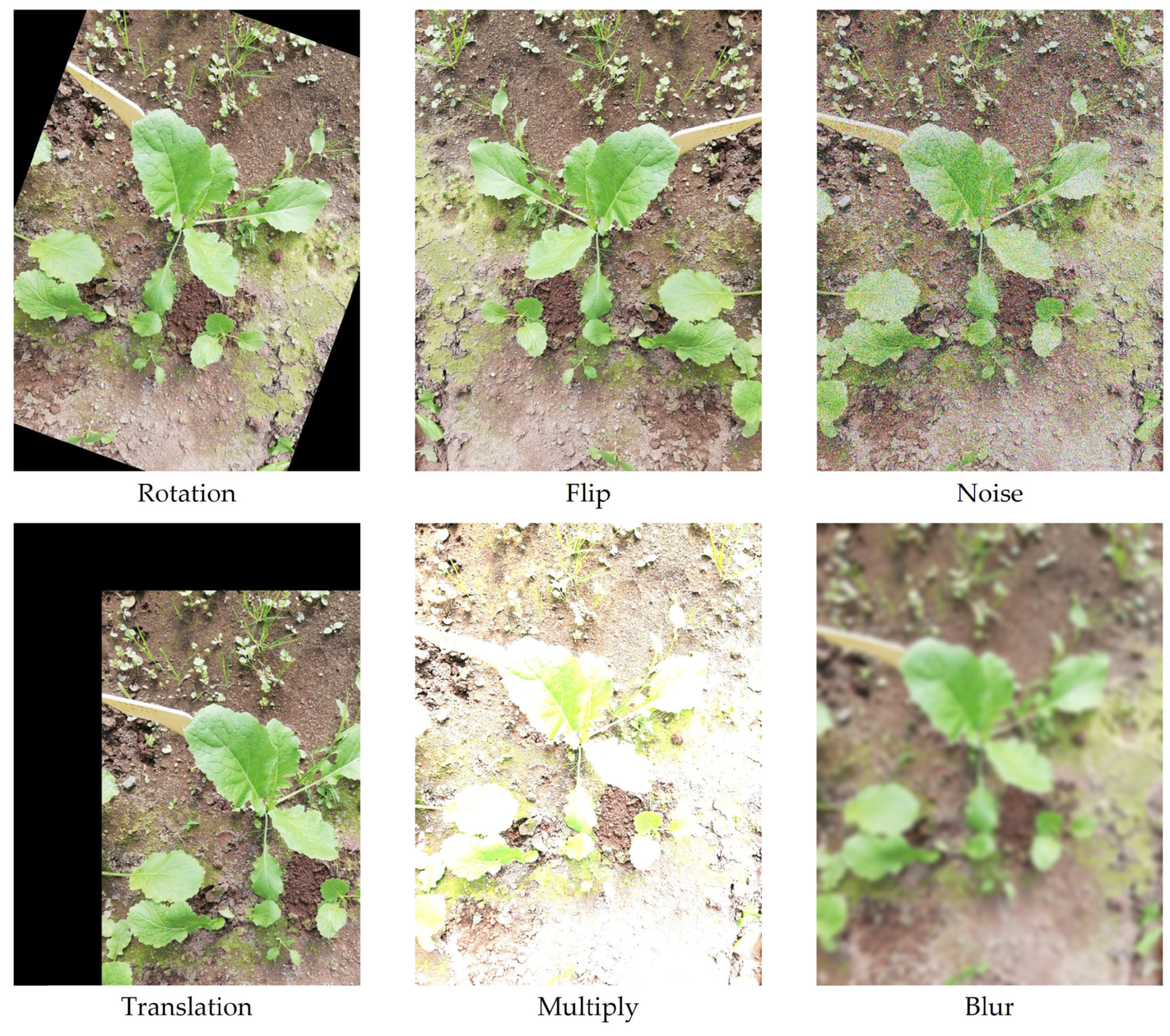
Data augmentation was used to increase the number of images, improving the overall learning procedure and performance by inputting variability into the dataset [23]. The transformations were carefully chosen, applying those that could happen under actual conditions, as displayed in Figure 2. The data transformations were applied to training and validation sets. The same transformations were applied to RGB images and the corresponding greyscale images (Table 4).
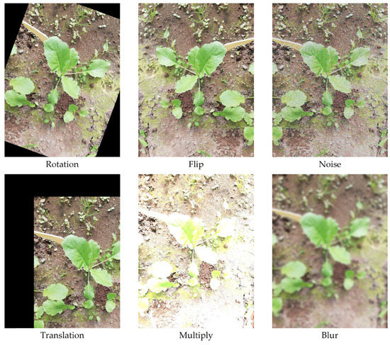
Figure 2.
Representation of the transformations applied to the images.

Table 4.
Training and validation image sets’ composition after the data augmentation step, considering only RGB images.
TensorFLow r.1.15.0 (see https://www.tensorflow.org/, last accessed: 13 October 2022) was used for the training and evaluation scripts of SSD models, whereas Darknet (see https://pjreddie.com/darknet/, last accessed: 14 October 2022) was used for YOLO v4. A GPU RTX3090 (VRAM of 24 GB) and a CPU Ryzen 9 5900X (12-core 3.7 GHz with a Turbo 4.8 GHz 70 MB SktAM4 with a RAM of 32 GB) were available to run the scripts.
Through transfer learning, pre-trained models with Microsoft’s COCO dataset (see https://cocodataset.org/, last accessed: 8 October 2022) were fine-tuned to classify vegetable crops’ phenophases. Some changes to the default training pipeline were made to optimise the training dynamics and generalisation ability, such as adjusting the batch size. The standard input size for each model was maintained with the addition of a variation of SSD MobileNet v2 with an input size of 300 × 300 px. This information is shown in Table 5.

Table 5.
Input and batch size for the training pipeline of the deep learning (DL) models tested.
Since data augmentation has already taken place, it was removed from the training pipeline. The SSD models’ training sessions ran for 50 000 steps, while the YOLO v4 training was conditioned by the number of classes of each crop (see https://github.com/AlexeyAB/darknet, last accessed: 4 November 2022). For example, YOLO v4 trained with lettuce (four classes) images ran for 8000 steps. An evaluation session occurred in the validation set according to the standard value used by the pre-trained models. These evaluation sessions are useful because they monitored the evolution of the training, i.e., detecting if the evaluation loss begins to increase while the training loss decreases or stays constant, which means that the model is excessively complex and cannot be well generalised to new data.
For benchmarking purposes, initially, training was carried out individually only with the RGB images corresponding to each crop and then replicated with greyscale images. After the individual performance evaluation of each model, the one that presented the best performance results was selected to be trained with all available data (RGB and greyscale images).
2.2.3. Models Performance Evaluation
The performance of the DL models was evaluated through a comparison between the predictions made by the DL model and the ground truth data of the position and phenophase of each plant. The following evaluation metrics were considered: F1-Score, mean average precision (mAP), and balanced accuracy (BA) [42,43,53].
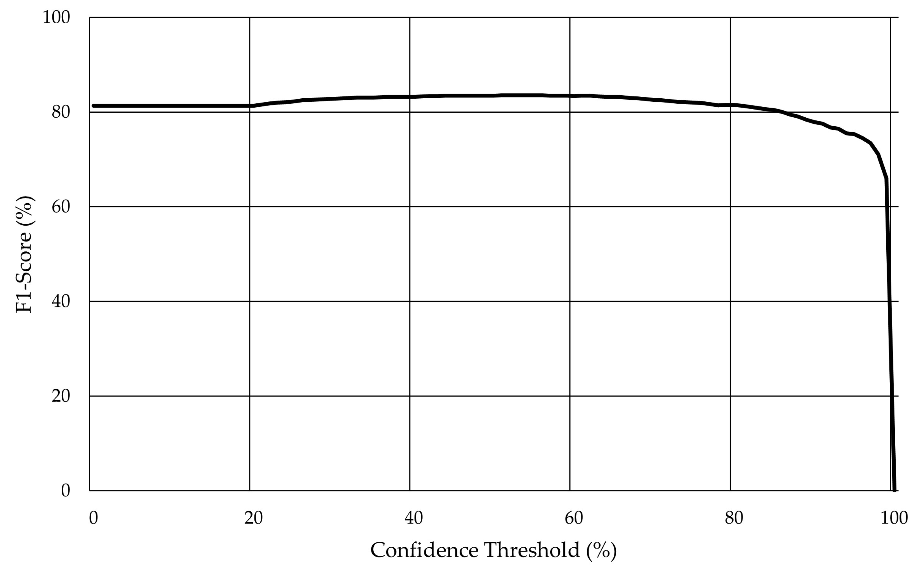
The cross-validation technique was applied according to Magalhães et al. [46] to optimise the DL model’s performance by optimising the confidence threshold. In the validation set, augmentations were removed, and the F1-Score was calculated for all the confidence thresholds from 0% to 100% into steps of 1%. The confidence threshold with the best F1-score output was selected for the model’s normal operation. The performance evaluation procedure considered the test set images and occurred in a GPU RTX3090 with a VRAM of 24 GB.
3. Results
Table 6 shows the results of the cross-validation technique applied to the validation set for both the models trained with RGB and greyscale images. The highest F1-score values are reported by SSD MobileNet v2 (300 × 300 px) and YOLO v4 trained with RGB and greyscale spinach images, respectively. SSD MobileNet v2 (300 × 300 px) trained with RGB carrot images and greyscale coriander images presented the lowest F1-scores of 58.4% and 32.0%, respectively. On average, the models with a higher F1-score are SSD ResNet 50 and YOLO v4, trained with RGB and greyscale images, respectively.

Table 6.
Confidence threshold that optimises the F1-score metric for each deep learning (DL) model tested in the validation set without augmentation.
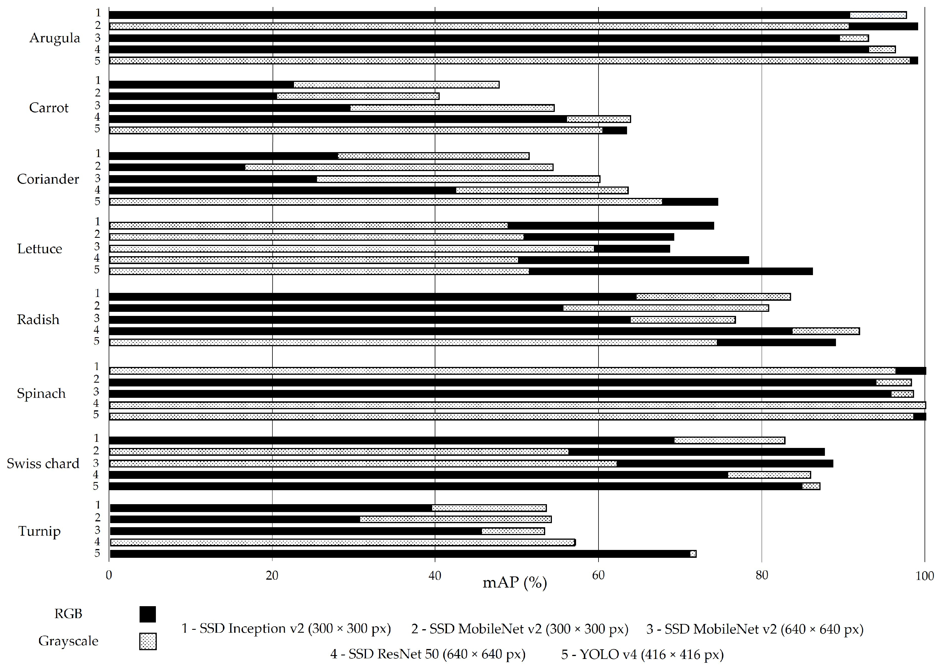
Figure 3 reports the mAP results for the best-computed confidence threshold. On average, this metric presents a value close to 70%, and the models trained with RGB images are slightly above (71.6%). Indeed, 25 of the 40 models trained with RGB images (solid black bars, Figure 3) present an mAP equal to or higher than the corresponding model trained with greyscale images (dashed bars, Figure 3).

Figure 3.
Mean average precision (mAP) for all models trained with RGB (solid black bars) and greyscale (dashed bars) images in the test set without augmentation.
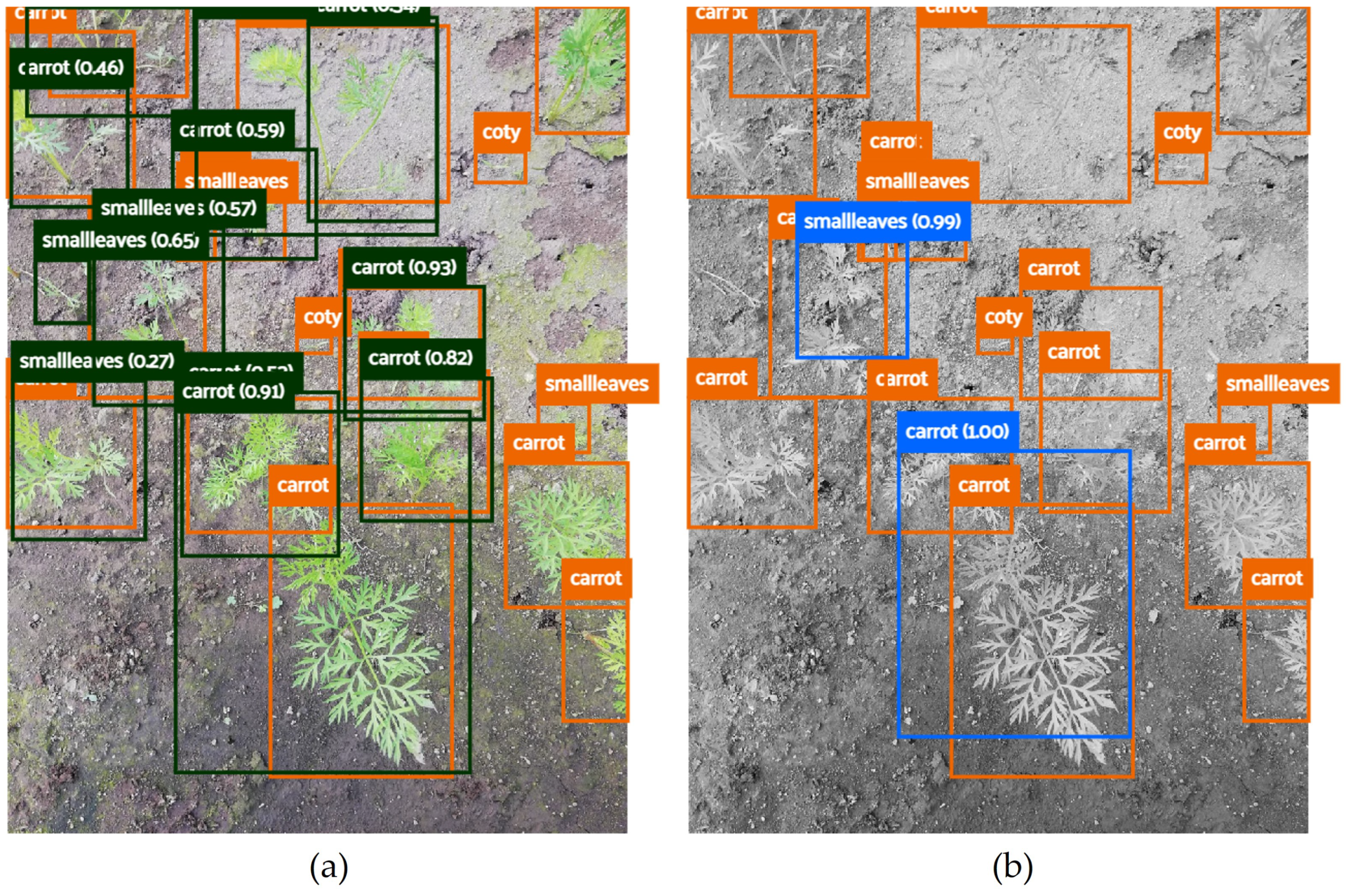
The models trained with carrot images present a lower mAP: close to 53% (RGB images) and 38% (greyscale images). Figure 4 shows the low performance of the SSD MobileNet v2 model (300 × 300 px) applied to carrot classification phenophases. This crop generally has erect and compound leaves (low soil cover), which facilitates weed growth and makes it more difficult to distinguish between the soil and plants (crop and weeds included).

Figure 4.
Carrot phenophase predictions made by SSD MobileNet v2 (300 × 300 px) using RGB (a) and the corresponding greyscale (b) image. Carrot phenophases are described as: coty (opened cotyledons), smallleaves (one to three unfolded leaves), and carrot (more than three unfolded leaves).
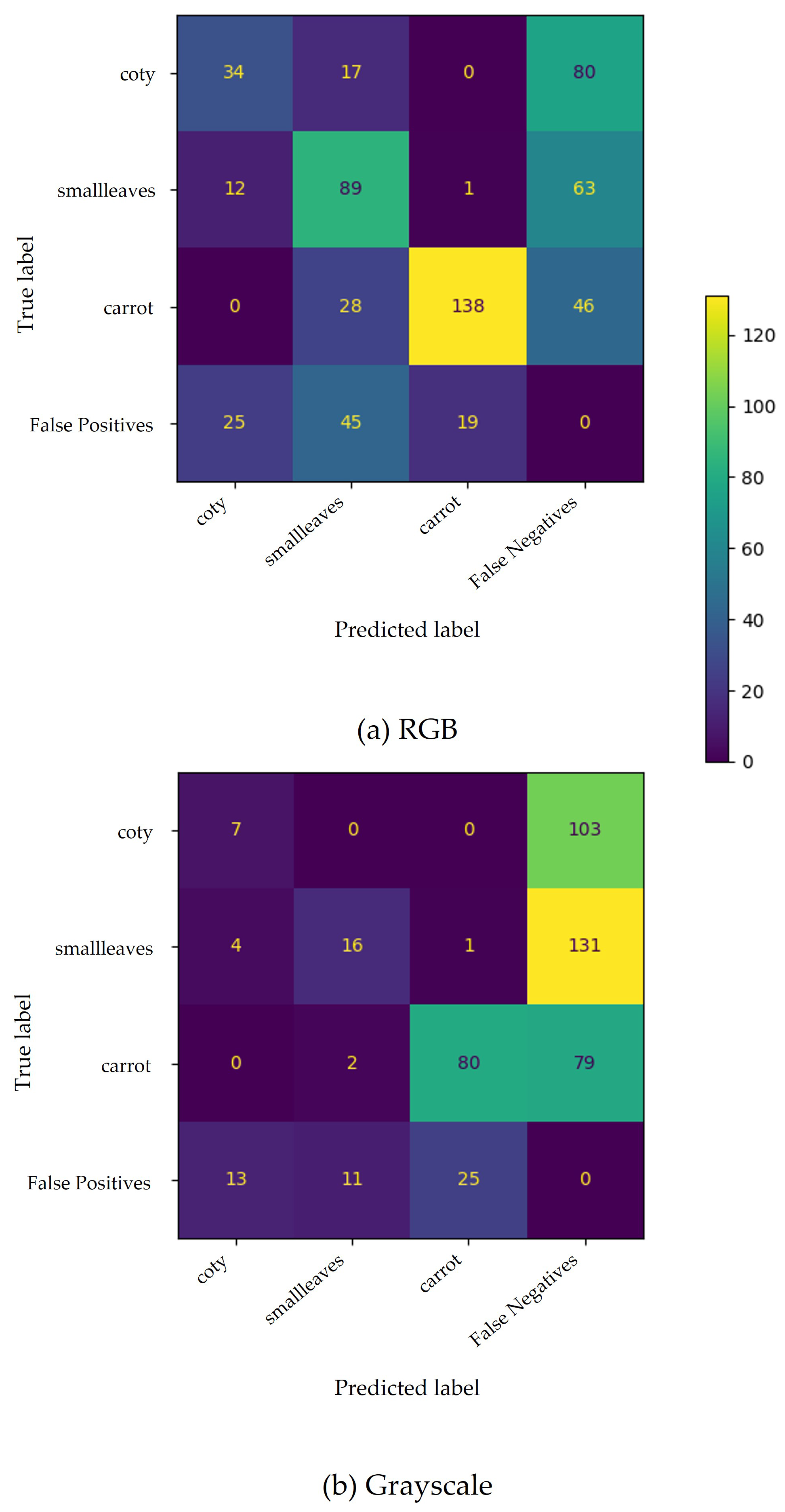
The confusion matrix (Figure 5) for SSD MobileNet v2 (300 × 300 px) shows low performance. The model had considerable difficulty locating the carrot plants, especially when trained with greyscale images, given the number of undetected ground truths (false negatives).

Figure 5.
Confusion matrix for carrots’ phenophases based on SSD MobileNet v2 (300 × 300 px) trained with RGB (a) and greyscale (b) images. False positives and false negatives include improperly predicted plants and undetected plants, respectively.
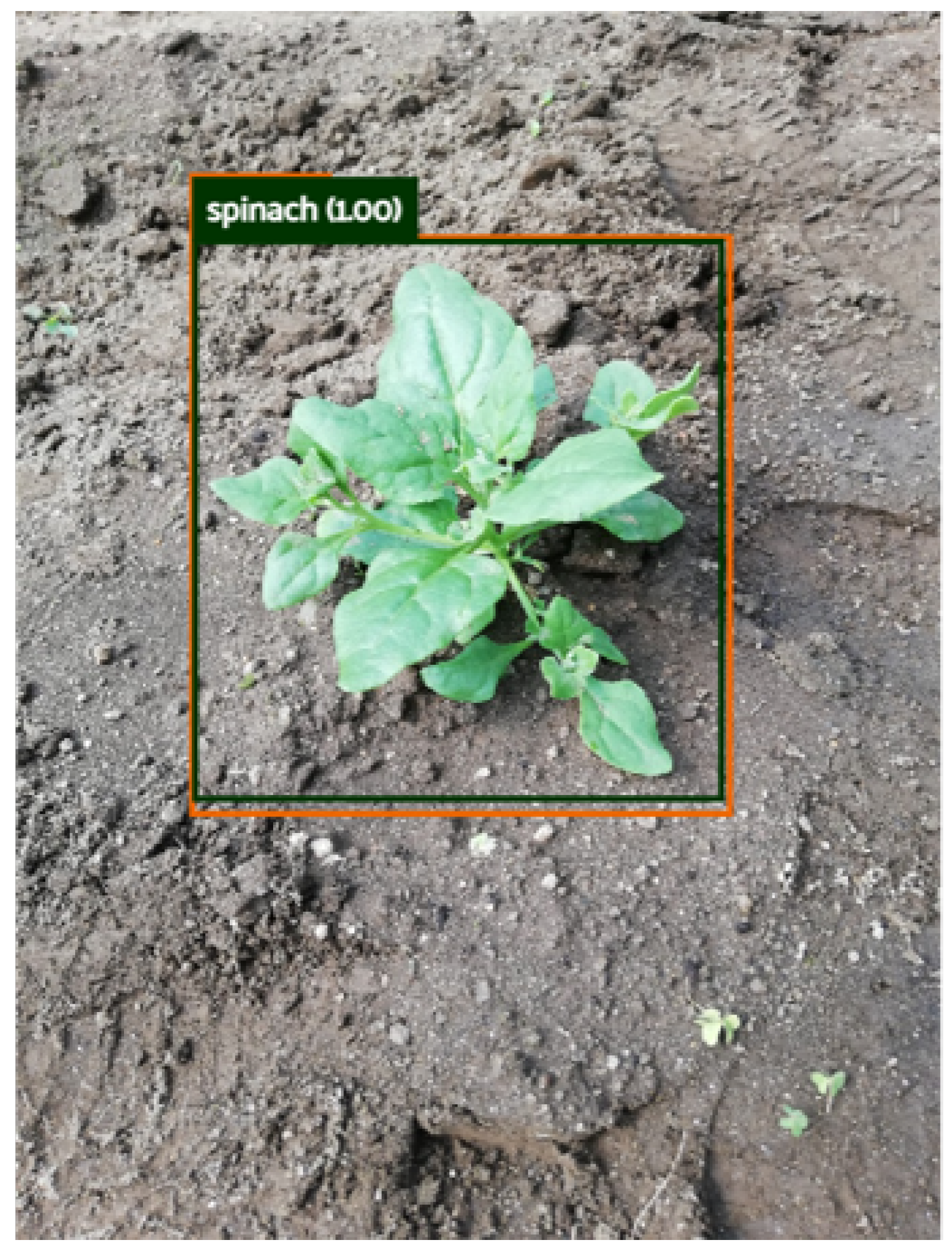
On the other hand, the models trained with spinach images are those with higher mAP (98.3% for RGB and 98.1% for greyscale images). The phenotypic traits of this crop test set may contribute to explaining the results. Figure 6 represents the spinach test set: images containing only one plant, with little weed or other plant presence and a clear distinction between the soil and the plant. Figure 6 is an example performed by ResNet 50, which was able to correctly classify all 57 ground truths of the test set.

Figure 6.
Spinach phenophase prediction made by SSD ResNet 50 based on RGB images. The spinach phenophase describes a spinach plant with less than nine unfolded leaves.
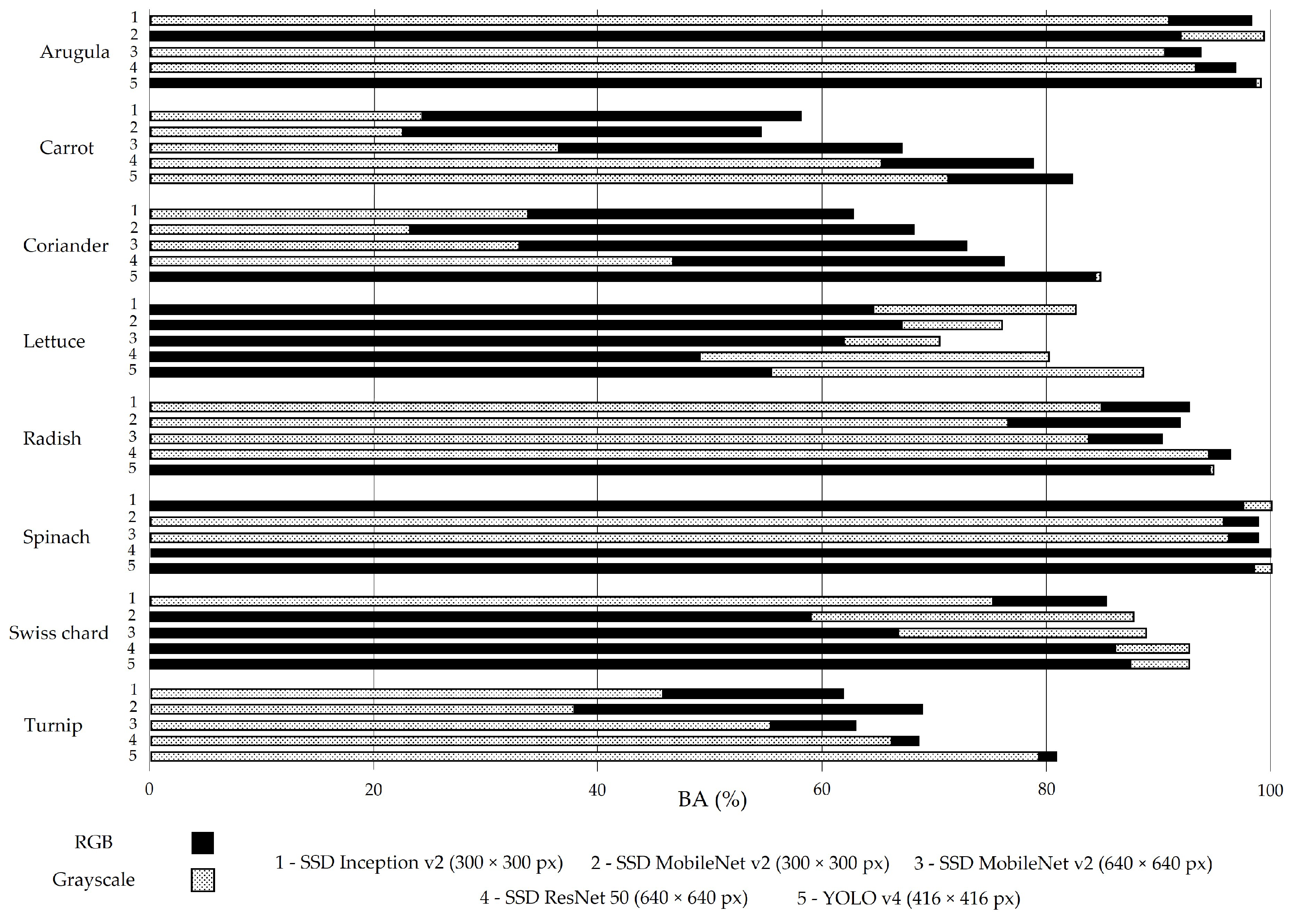
The BA metric presented in Figure 7 is close to 77% (RGB images) and 79.2% (greyscale images), which are similar to the results of mAP (Figure 3).
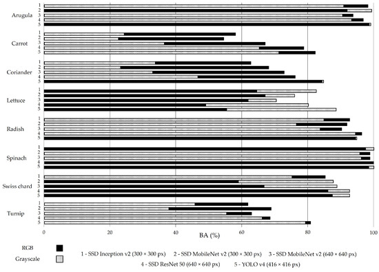
Figure 7.
Balanced accuracy (BA) for all models trained with RGB (solid black bars) and greyscale (dashed bars) images in the test set without augmentation.
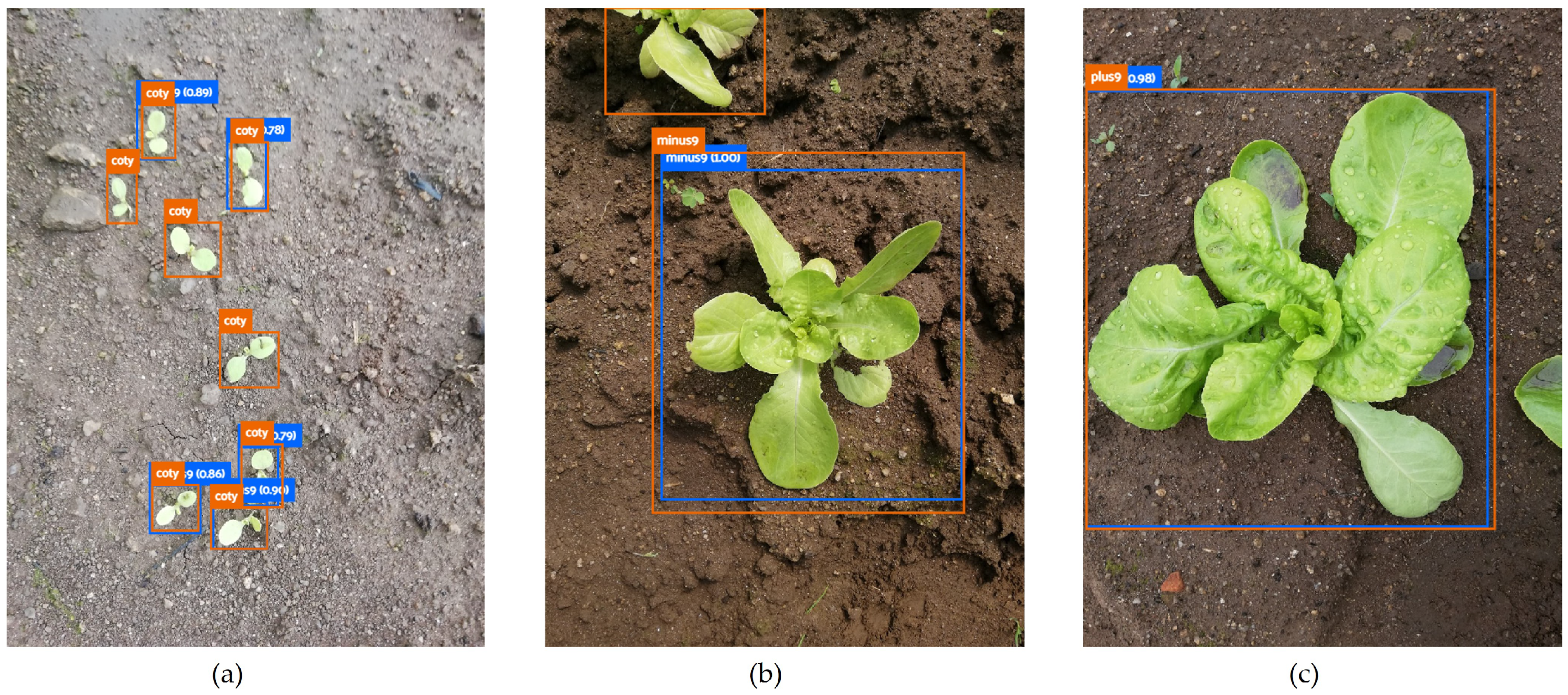
The importance of BA relies on two aspects: it allows one to overcome biased conclusions due to unbalanced datasets [53] and it enables the analysis of correctly located objects, regardless of whether they are accurately classified. The latter is of particular interest in this work, as it is difficult, even for a skilled observer, to identify plants as small as cotyledons (Figure 8a) or to distinguish whether a plant has less (Figure 8b) or more (Figure 8c) than nine leaves.
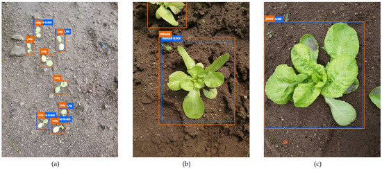
Figure 8.
Lettuce phenophases: (a) coty (opened cotyledons); (b) minus9 (less than nine unfolded leaves); (c) plus9 (nine or more unfolded leaves).
SSD ResNet 50 was the best-performing SSD model for both image groups, which is reflected not only in mAP results (76.0% for RGB and 73.3% for greyscale images) but also in BA results (81.4% for RGB and 79.8% for greyscale images).
However, SSD models have been outperformed by YOLO v4. This DL model presents, for both groups of images, not only a better performance when the analysis is based on mAP (76.2% for RGB and 83.5% for greyscale images) but also when the evaluation relies on BA (85.2% for RGB and 88.8% for greyscale images). Supported by these results, it was decided to train the YOLO v4 (416 × 416 px) model with all the images of the 24 defined phenophases, representing the growing season of the eight vegetable crops selected for the dataset construction. The dataset split resulted in 54,090 images for training, 19,532 images for validation, and 1524 images for test sets. The training and validation sets include the images resulting from the augmentation procedure.
As previously mentioned, Darknet was used for the training and evaluation scripts, and the model training session ran for 48,000 steps. Furthermore, cross-validation (Figure 9) was applied with the model achieving an F1-Score of 83.6% for a confidence threshold higher than 53%.
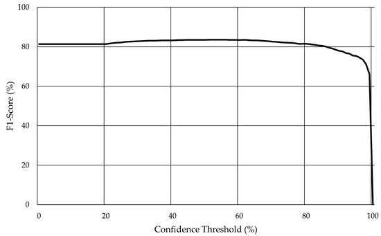
Figure 9.
Evolution of the F1-score with the variation of the confidence threshold for YOLO v4 in the validation set without augmentation.
The following performance analysis, summarised in Table 7, was conducted on the test set, considering the best-computed confidence rate (53%). The overall performance remained consistent, except for the slight differences compared with the average values of the YOLO v4 variations trained with the independent image groups.

Table 7.
Different evaluation metrics results for YOLO v4 model variations.
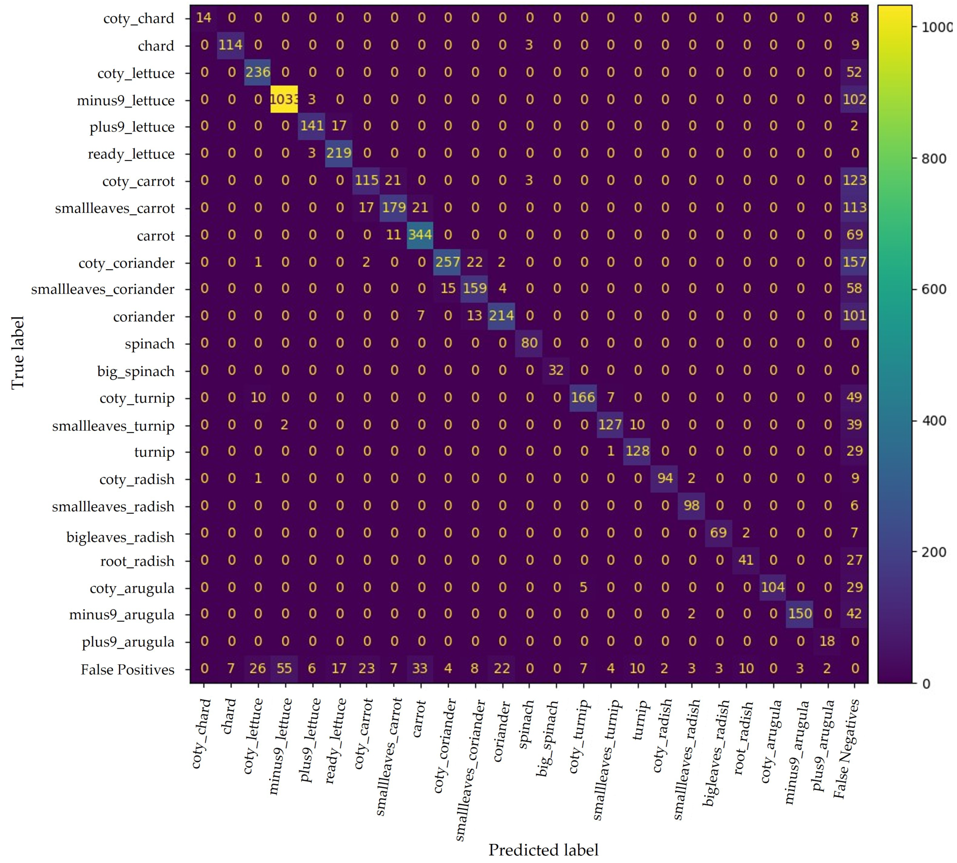
The confusion matrix in Figure 10 shows YOLO v4 performance. This DL model could discretise the phenotypic traits of the different phenophases for successful classification. The model was able to correctly classify 4123 plants out of a total of 5396 ground truths (Table 2).
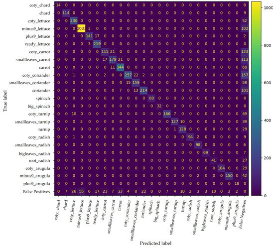
Figure 10.
Confusion matrix for YOLO v4 trained with all available data. False positives and false negatives include improperly predicted plants and undetected plants, respectively.
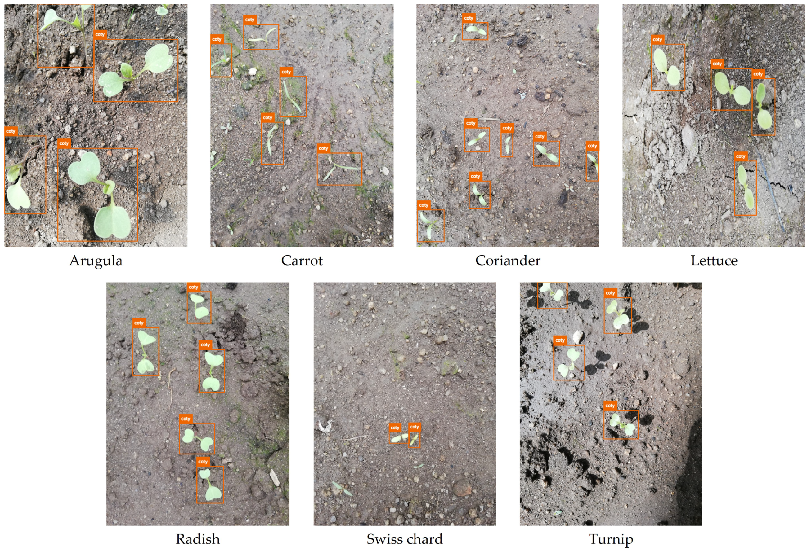
Nevertheless, some phenophases have similar phenotypic traits, leading to misclassifications. For instance, the coty class is present in all crops except spinach, which presents similar morphological traits as those seen in Figure 11. Nevertheless, the number of false positives only between predictions in this class is relatively low, yet the respective number of false negatives cannot be neglected. Hence, the resulting mAP for coty is approximately 67%.

Figure 11.
Examples of coty class images from the dataset under study.
4. Discussion
Overall, both architectures were generic enough to successfully classify the vegetables’ phenophases. SSD ResNet 50 was the best-performing SSD model for both image groups individually, and SSD MobileNet v2 (640 × 640 px) performed slightly better than the variation SSD MobileNet v2 (300 × 300 px), suggesting that the performance of this architecture is favoured by increasing the input size. The proposed SSD MobileNet v2 models outperformed the one presented by d’Andrimont et al. [31], which obtained an mAP close to 55%.
The results presented by the SSD ResNet 50 model align with those shown by Ofori et al. [39], where this model performed better than other DL models, including SSD Inception v2. Pearse et al. [35] and Samiei et al. [40] presented the ResNet model variations that performed slightly better than that proposed in this study (98% and 90%, respectively). However, the former application was for the well-defined Metrosideros excelsa flowering phenophase classification, and the latter used a dataset that did not represent actual conditions since the soil background was removed from the images.
YOLO v4 was the model that presented a more consistent performance in both image groups. Hence, it was trained with all the images available in the dataset. The model performance was not significantly impacted, remaining close to 77% and 82% for mAP and BA, respectively. To the best of our knowledge, no work has tested a YOLO model for phenology monitoring. Correia et al. [36] is the only study where an object detector was developed, with lower performance when compared with the proposed YOLO v4 model.
The greyscale transformation did not significantly hinder the models’ performance, the differences being more notorious on the SSD Inception v2 and smaller on YOLO v4, where even the models trained with greyscale images showed a better performance.
Furthermore, the DL models’ performance was not homogeneous with regard to different crops, with the models trained with carrot images and those trained with spinach images being the lowest and highest extremes, respectively. In this case, and in line with different authors [29,30], the images’ quantity and quality, particularly the specific phenotypic traits of each crop, may compromise the results.
The models could classify vegetables at different phenological phases, even in non-structured environments, considering overlaps and variable sunlight conditions. For the comprehensive tracking of the crop cycle, it is crucial to monitor the phenology right after the cotyledons’ appearance and opening. Regarding coty (cotyledons’ opening), YOLO v4 classified this phenophase with an mAP of approximately 67%. Although slightly lower than the results reported by the literature [39,40], it is important to highlight that, in contrast to these, the images applied in this study represent actual conditions, without pre-processing operations, such as segmentation, to differentiate the plants.
5. Conclusions
This paper presents a benchmark of four DL models for assessing the capability of CNN to leverage phenological classification in vegetable crops. A dataset with 4123 images was manually collected during various growing seasons of eight vegetable crops representing the main phenophases from emergence to harvest. For benchmarking purposes, each model was tested for the classification of each crop individually. YOLO v4 was the best-performing model compared to the SSD models. Therefore, this model was tested with all data obtaining a mAP of 76.6% and a BA of 81.7%.
All assessed models delivered promising results, and were able to classify the phenological phases of individual plants between emergence and harvest. Furthermore, a single DL model could classify multiple vegetable crops considering phenology dynamics throughout the growing season at the subfield scale. As far as we have been able to ascertain, this is the first study to evaluate the potential of CV_DL for vegetable crops’ phenological research. Notwithstanding some limitations, this work is an important step towards sustainable agricultural practices.
Further work needs to be done to (i) enlarge the dataset, balancing it with more images within less populated phenophases and increasing the number of vegetable crops; and (ii) assess the inference speed of the proposed models before transferring the detection framework to a robotic-assisted CV platform, thus allowing a more rigorous image collection as well as a more accurate ground truth identification; (iii) extend the benchmark with a new and more optimised backbone network, such as YOLO v7, and different DL architectures, such as faster R-CNN, confirming whether the SSD and YOLO architectures maintain better performance; and (iv) perform an ablation study in the best-performing model, YOLO v4, to understand the model behaviour and measure the contribution of each model component to the overall model performance.
Furthermore, the proposed CV_DL framework can be framed in a modelling approach estimating the extent to which genetic, environmental, and management conditions impact the timing of phenophases and how they affect the efficiency of agricultural practices and crop yield.
Author Contributions
Conceptualisation, L.R., M.C. and F.N.d.S.; data curation, L.R.; investigation, L.R.; methodology, L.R., S.A.M. and D.Q.d.S.; software, L.R., S.A.M. and D.Q.d.S.; supervision, M.C. and F.N.d.S.; validation, M.C. and F.N.d.S.; visualisation, L.R.; writing—original draft, L.R.; writing—review and editing, S.A.M., D.Q.d.S., M.C. and F.N.d.S. All authors read and agreed to the published version of the manuscript.
Funding
This work is partially financed by National Funds through the FCT—Fundação para a Ciência e a Tecnologia, I.P. (Portuguese Foundation for Science and Technology) within the project OmicBots, with reference PTDC/ASP-HOR/1338/2021. Besides, this work has received funding from the European Union’s Horizon 2020 research and innovation programme under grant agreement No. 857202.
Institutional Review Board Statement
Not applicable.
Informed Consent Statement
Not applicable.
Data Availability Statement
The data presented in this study are openly available in the digital repository Zenodo: PixelCropRobot Dataset—https://doi.org/10.5281/zenodo.7433286 (last accessed: 5 November 2022).
Acknowledgments
The authors would like to acknowledge the scholarships 9684/BI-M-ED_B2/2022 (L.R.), SFRH/BD/147117/2019 (S.A.M.), and UI/BD/152564/2022 (D.Q.d.S.) funded by National Funds through the Portuguese funding agency, FCT—Fundação para a Ciência e Tecnologia.
Conflicts of Interest
The authors declare no conflict of interest. The funders had no role in the design of the study; in the collection, analyses, or interpretation of data; in the writing of the manuscript, or in the decision to publish the results.
References
- Lieth, H. Phenology and Seasonality Modeling. In Ecological Studies; Springer: Berlin/Heidelberg, Germany, 1974. [Google Scholar] [CrossRef]
- Liang, L. Phenology. In Reference Module in Earth Systems and Environmental Sciences; Elsevier: Amsterdam, The Netherlands, 2019. [Google Scholar] [CrossRef]
- Ruml, M.; Vulić, T. Importance of phenological observations and predictions in agriculture. J. Agric. Sci. 2005, 50, 217–225. [Google Scholar] [CrossRef]
- Chmielewski, F.M. Phenology in Agriculture and Horticulture. In Phenology: An Integrative Environmental Science; Schwartz, M.D., Ed.; Springer: Dordrecht, The Netherlands, 2013; pp. 539–561. [Google Scholar] [CrossRef]
- Martín-Forés, I.; Casado, M.A.; Castro, I.; del Pozo, A.; Molina-Montenegro, M.; Miguel, J.M.D.; Acosta-Gallo, B. Variation in phenology and overall performance traits can help to explain the plant invasion process amongst Mediterranean ecosystems. NeoBiota 2018, 41, 67–89. [Google Scholar] [CrossRef]
- Kato, A.; Carlson, K.M.; Miura, T. Assessing the inter-annual variability of vegetation phenological events observed from satellite vegetation index time series in dryland sites. Ecol. Indic. 2021, 130, 108042. [Google Scholar] [CrossRef]
- Kasampalis, D.A.; Alexandridis, T.K.; Deva, C.; Challinor, A.; Moshou, D.; Zalidis, G. Contribution of Remote Sensing on Crop Models: A Review. J. Imaging 2018, 4, 52. [Google Scholar] [CrossRef]
- Fu, Y.; Li, X.; Zhou, X.; Geng, X.; Guo, Y.; Zhang, Y. Progress in plant phenology modeling under global climate change. Sci. China Earth Sci. 2020, 63, 1237–1247. [Google Scholar] [CrossRef]
- Kephe, P.; Ayisi, K.; Petja, B. Challenges and opportunities in crop simulation modelling under seasonal and projected climate change scenarios for crop production in South Africa. Agric. Food Secur. 2021, 10, 10. [Google Scholar] [CrossRef]
- Hufkens, K.; Melaas, E.K.; Mann, M.L.; Foster, T.; Ceballos, F.; Robles, M.; Kramer, B. Monitoring crop phenology using a smartphone based near-surface remote sensing approach. Agric. For. Meteorol. 2019, 265, 327–337. [Google Scholar] [CrossRef]
- Guo, Y.; Chen, S.; Fu, Y.H.; Xiao, Y.; Wu, W.; Wang, H.; Beurs, K.d. Comparison of Multi-Methods for Identifying Maize Phenology Using PhenoCams. Remote Sens. 2022, 14, 244. [Google Scholar] [CrossRef]
- Chacón-Maldonado, A.M.; Molina-Cabanillas, M.A.; Troncoso, A.; Martínez-Álvarez, F.; Asencio-Cortés, G. Olive Phenology Forecasting Using Information Fusion-Based Imbalanced Preprocessing and Automated Deep Learning. In Proceedings of the Hybrid Artificial Intelligent Systems Conference, Salamanca, Spain, 5–7 September 2022. [Google Scholar] [CrossRef]
- Milicevic, M.; Zubrinic, K.; Grbavac, I.; Obradovic, I. Application of Deep Learning Architectures for Accurate Detection of Olive Tree Flowering Phenophase. Remote Sens. 2020, 12, 2120. [Google Scholar] [CrossRef]
- Jing, H.; Xiujuan, W.; Haoyu, W.; Xingrong, F.; Mengzhen, K. Prediction of crop phenology—A component of parallel agriculture management. In Proceedings of the 2017 Chinese Automation Congress, Jinan, China, 20–22 October 2017; pp. 7704–7708. [Google Scholar] [CrossRef]
- Giordano, M.; Petropoulos, S.A.; Rouphael, Y. Response and Defence Mechanisms of Vegetable Crops against Drought, Heat and Salinity Stress. Agriculture 2021, 11, 463. [Google Scholar] [CrossRef]
- Dhondt, S.; Wuyts, N.; Inzé, D. Cell to whole-plant phenotyping: The best is yet to come. Trends Plant Sci. 2013, 18, 428–439. [Google Scholar] [CrossRef]
- Tripathi, M.K.; Maktedar, D.D. A role of computer vision in fruits and vegetables among various horticulture products of agriculture fields: A survey. Inf. Process. Agric. 2020, 7, 183–203. [Google Scholar] [CrossRef]
- Patrício, D.I.; Rieder, R. Computer vision and artificial intelligence in precision agriculture for grain crops: A systematic review. Comput. Electron. Agric. 2018, 153, 69–81. [Google Scholar] [CrossRef]
- Narvaez, F.; Reina, G.; Torres-Torriti, M.; Kantor, G.; Cheein, F. A Survey of Ranging and Imaging Techniques for Precision Agriculture Phenotyping. IEEE/ASME Trans. Mechatron. 2017, 22, 2428–2439. [Google Scholar] [CrossRef]
- Roy, A.M.; Bose, R.; Bhaduri, J. A fast accurate fine-grain object detection model based on YOLOv4 deep neural network. Neural Comput. Appl. 2022, 34, 1–27. [Google Scholar] [CrossRef]
- Jin, X.; Che, J.; Chen, Y. Weed Identification Using Deep Learning and Image Processing in Vegetable Plantation. IEEE Access 2021, 9, 10940–10950. [Google Scholar] [CrossRef]
- Aguiar, A.S.; Magalhães, S.A.; dos Santos, F.N.; Castro, L.; Pinho, T.; Valente, J.; Martins, R.; Boaventura-Cunha, J. Grape bunch detection at different growth stages using deep learning quantized models. Agronomy 2021, 11, 1890. [Google Scholar] [CrossRef]
- Kamilaris, A.; Prenafeta-Boldú, F.X. Deep learning in agriculture: A survey. Comput. Electron. Agric. 2018, 147, 70–90. [Google Scholar] [CrossRef]
- Yang, B.; Xu, Y. Applications of deep-learning approaches in horticultural research: A review. Hortic. Res. 2021, 8, 123. [Google Scholar] [CrossRef]
- Katal, N.; Rzanny, M.; Mäder, P.; Wäldchen, J. Deep Learning in Plant Phenological Research: A Systematic Literature Review. Front. Plant Sci. 2022, 13, 805738. [Google Scholar] [CrossRef]
- Potgieter, A.B.; Zhao, Y.; Zarco-Tejada, P.J.; Chenu, K.; Zhang, Y.; Porker, K.; Biddulph, B.; Dang, Y.P.; Neale, T.; Roosta, F.; et al. Evolution and application of digital technologies to predict crop type and crop phenology in agriculture. Silico Plants 2021, 3, diab017. [Google Scholar] [CrossRef]
- Yang, W.; Feng, H.; Zhang, X.; Zhang, J.; Doonan, J.; Batchelor, W.D.; Xiong, L.; Yan, J. Crop Phenomics and High-Throughput Phenotyping: Past Decades, Current Challenges, and Future Perspectives. Mol. Plant 2020, 13, 187–214. [Google Scholar] [CrossRef] [PubMed]
- Arya, S.; Sandhu, K.S.; Singh, J. Deep learning: As the new frontier in high-throughput plant phenotyping. Euphytica 2022, 218, 1–22. [Google Scholar] [CrossRef]
- Yalcin, H. Plant phenology recognition using deep learning: Deep-Pheno. In Proceedings of the 6th International Conference on Agro-Geoinformatics, Fairfax, VA, USA, 7–10 August 2017; pp. 1–5. [Google Scholar] [CrossRef]
- Han, J.; Shi, L.; Yang, Q.; Huang, K.; Zha, Y.; Jin, Y. Real-time detection of rice phenology through convolutional neural network using handheld camera images. Precis. Agric. 2021, 22, 154–178. [Google Scholar] [CrossRef]
- d’Andrimont, R.; Yordanov, M.; Martinez-Sanchez, L.; van der Velde, M. Monitoring crop phenology with street-level imagery using computer vision. Comput. Electron. Agric. 2022, 196, 106866. [Google Scholar] [CrossRef]
- Taylor, S.D.; Browning, D.M. Classification of Daily Crop Phenology in PhenoCams Using Deep Learning and Hidden Markov Models. Remote Sens. 2022, 14, 286. [Google Scholar] [CrossRef]
- Wang, X.; Tang, J.; Whitty, M. DeepPhenology: Estimation of apple flower phenology distributions based on deep learning. Comput. Electron. Agric. 2021, 185, 106123. [Google Scholar] [CrossRef]
- Molina, M.Á.; Jiménez-Navarro, M.J.; Martínez-Álvarez, F.; Asencio-Cortés, G. A Model-Based Deep Transfer Learning Algorithm for Phenology Forecasting Using Satellite Imagery. In Proceedings of the Hybrid Artificial Intelligent Systems, Bilbao, Spain, 22–24 September 2021; pp. 511–523. [Google Scholar] [CrossRef]
- Pearse, G.; Watt, M.S.; Soewarto, J.; Tan, A.Y. Deep Learning and Phenology Enhance Large-Scale Tree Species Classification in Aerial Imagery during a Biosecurity Response. Remote Sens. 2021, 13, 1789. [Google Scholar] [CrossRef]
- Correia, D.L.; Bouachir, W.; Gervais, D.; Pureswaran, D.; Kneeshaw, D.D.; De Grandpré, L. Leveraging Artificial Intelligence for Large-Scale Plant Phenology Studies From Noisy Time-Lapse Images. IEEE Access 2020, 8, 13151–13160. [Google Scholar] [CrossRef]
- Mann, H.M.R.; Iosifidis, A.; Jepsen, J.U.; Welker, J.M.; Loonen, M.J.J.E.; Høye, T.T. Automatic flower detection and phenology monitoring using time-lapse cameras and deep learning. Remote Sens. Ecol. Conserv. 2022, 8, 765–777. [Google Scholar] [CrossRef]
- Chavan, T.; Nandedkar, A. AgroAVNET for crops and weeds classification: A step forward in automatic farming. Comput. Electron. Agric. 2018, 154, 361–372. [Google Scholar] [CrossRef]
- Ofori, M.; El-Gayar, O. Towards Deep Learning for Weed Detection: Deep Convolutional Neural Network Architectures for Plant Seedling Classification. In Proceedings of the Americas Conference on Information Systems, Virtual, 10–14 August 2020. [Google Scholar]
- Samiei, S.; Rasti, P.; Vu, J.; Buitink, J.; Rousseau, D. Deep learning-based detection of seedling development. Plant Methods 2020, 16, 103. [Google Scholar] [CrossRef]
- Meier, U. (Ed.) Growth Stages of Mono- and Dicotyledonous Plants; Julius Kühn-Institut: Quedlinburg, Germany, 2018. [Google Scholar]
- Everingham, M.; Gool, L.V.; Williams, C.K.I.; Winn, J.M.; Zisserman, A. The Pascal Visual Object Classes (VOC) Challenge. Int. J. Comput. Vis. 2010, 88, 303–338. [Google Scholar] [CrossRef]
- Padilla, R.; Passos, W.L.; Dias, T.L.B.; Netto, S.L.; da Silva, E.A.B. A Comparative Analysis of Object Detection Metrics with a Companion Open-Source Toolkit. Electronics 2021, 10, 279. [Google Scholar] [CrossRef]
- Terra, F.; Rodrigues, L.; Magalhães, S.; Santos, F.; Moura, P.; Cunha, M. PixelCropRobot, a cartesian multitask platform for microfarms automation. In Proceedings of the 2021 International Symposium of Asian Control Association on Intelligent Robotics and Industrial Automation (IRIA), Goa, India, 20–22 September 2021; pp. 382–387. [Google Scholar] [CrossRef]
- Liu, W.; Anguelov, D.; Erhan, D.; Szegedy, C.; Reed, S.; Fu, C.Y.; Berg, A.C. SSD: Single Shot MultiBox Detector. Lect. Notes Comput. Sci. 2016, 9905, 21–37. [Google Scholar] [CrossRef]
- Magalhães, S.A.; Castro, L.; Moreira, G.; dos Santos, F.N.; Cunha, M.; Dias, J.; Moreira, A.P. Evaluating the Single-Shot MultiBox Detector and YOLO Deep Learning Models for the Detection of Tomatoes in a Greenhouse. Sensors 2021, 21, 3569. [Google Scholar] [CrossRef]
- Moreira, G.; Magalhães, S.A.; Pinho, T.; dos Santos, F.N.; Cunha, M. Benchmark of Deep Learning and a Proposed HSV Colour Space Models for the Detection and Classification of Greenhouse Tomato. Agronomy 2022, 12, 356. [Google Scholar] [CrossRef]
- Ioffe, S.; Szegedy, C. Batch Normalization: Accelerating Deep Network Training by Reducing Internal Covariate Shift. In Proceedings of the 32nd International Conference on International Conference on Machine Learning, Lille, France, 6–11 July 2015; pp. 448–456. [Google Scholar]
- Szegedy, C.; Liu, W.; Jia, Y.; Sermanet, P.; Reed, S.; Anguelov, D.; Erhan, D.; Vanhoucke, V.; Rabinovich, A. Going deeper with convolutions. In Proceedings of the Conference on Computer Vision and Pattern Recognition, Boston, MA, USA, 7–12 June 2015; pp. 1–9. [Google Scholar] [CrossRef]
- Sandler, M.; Howard, A.; Zhu, M.; Zhmoginov, A.; Chen, L.C. MobileNetV2: Inverted Residuals and Linear Bottlenecks. In Proceedings of the Conference on Computer Vision and Pattern Recognition, Salt Lake City, UT, USA, 18–22 June 2018; pp. 4510–4520. [Google Scholar] [CrossRef]
- He, K.; Zhang, X.; Ren, S.; Sun, J. Deep Residual Learning for Image Recognition. In Proceedings of the 2016 IEEE Conference on Computer Vision and Pattern Recognition, Las Vegas, NV, USA, 26 June–1 July 2016; pp. 770–778. [Google Scholar] [CrossRef]
- Bochkovskiy, A.; Wang, C.Y.; Liao, H.Y.M. YOLOv4: Optimal speed and accuracy of object detection. arXiv 2020. [Google Scholar] [CrossRef]
- Brodersen, K.H.; Ong, C.S.; Stephan, K.E.; Buhmann, J.M. The Balanced Accuracy and Its Posterior Distribution. In Proceedings of the 20th International Conference on Pattern Recognition, Istanbul, Turkey, 23–26 August 2010; pp. 3121–3124. [Google Scholar] [CrossRef]
Disclaimer/Publisher’s Note: The statements, opinions and data contained in all publications are solely those of the individual author(s) and contributor(s) and not of MDPI and/or the editor(s). MDPI and/or the editor(s) disclaim responsibility for any injury to people or property resulting from any ideas, methods, instructions or products referred to in the content. |
© 2023 by the authors. Licensee MDPI, Basel, Switzerland. This article is an open access article distributed under the terms and conditions of the Creative Commons Attribution (CC BY) license (https://creativecommons.org/licenses/by/4.0/).

