Economic Evaluation and Risk Premium Estimation of Rainfed Soybean under Various Planting Practices in a Semi-Humid Drought-Prone Region of Northwest China

Abstract

Economic benefits and risk premiums significantly affect the production system decision making of farmers and government departments. This study evaluated the economic feasibility and estimated the risk premium of 12 rainfed soybean production systems with various planting densities, fertilization rates and planting patterns by considering the impact of soybean price fluctuation. There were two planting densities (D₁: 160,000 plants ha⁻¹ and D₂: 320,000 plants ha⁻¹), two fertilization rates (F₁: 20 kg ha⁻¹ N, 30 kg ha⁻¹ P, 30 kg ha⁻¹ K; F₂: 40 kg ha⁻¹ N, 60 kg ha⁻¹ P, 60 kg ha⁻¹ K) and three planting patterns (F+W₀: flat cultivation with no irrigation; R+W₀: plastic-mulched ridge-furrow cultivation (PMRF) with no irrigation; R+W₁: PMRF with supplemental irrigation of 30 mm at the pod-filling stage). Based on the two-year (2019–2020) field data in a semi-humid drought-prone region of northwest China and soybean price fluctuation from January 2014 to June 2021, the net income (NI) was calculated by considering the impact of soybean price fluctuation and assuming constant soybean production costs. The net present value (NPV) method and the stochastic efficiency with respect to a function (SERF) method were used to evaluate the profitability of protective alternatives and the risk of these alternatives. The results showed that the 12 proposed soybean production systems were economically feasible. Reducing the fertilization rate reduced the input costs, but it did not necessarily result in a decrease in soybean yield and NI. The payback period of all production systems was within two years for farmers investing through loans. High-fertilizer and high-density production systems made personal investment obtain the highest economic benefit in this study, which was not the best investment strategy from the perspective of production-to-investment ratio and environmental protection departments. The preferences of farmers with various risk aversion and environmental protection departments in terms of risk premium were also proposed. The economic and risk assessment framework of this study can enhance the understanding of the adjustment of production systems from different perspectives, and provide strategies for promoting the protection of economic, environmental and socially sustainable agricultural systems.

1. Introduction

Soybean (Glycine max L. Merr) is one of the most important sources of protein and oil, and it is the fourth most important crop around the world in terms of seed production [1]. China is one of the four largest soybean-producing countries in the world, and Chinese soybean production has a great impact on the global market. However, the seasonal fluctuation in production and price fluctuation caused by various risks affect the soybean market, thereby further adjusting soybean prices. The fluctuation of soybean prices has a great impact on farmers’ incomes.

Crops are highly exposed to various types of risk, i.e., climate risk, biological risk, price risk and financial risk [2,3]. Soybean is one of the major crops widely planted in northwest China [4], and the soybean planting system in the semi-humid drought-prone regions of northwest China is highly dependent on climatic conditions, planting patterns and production systems, which affect farmers’ NI. As climate change intensifies, soybean production in Northwest China will be affected, which will also affect soybean prices and economic profitability [5]. Risks from extreme weather events to crop production can be mitigated through the adoption of innovative management strategies [6]. Incorporating plastic-mulched ridge-furrow cultivation (PMRF) into the planting system is a useful management option to maintain and increase soil moisture and soil temperature and promote crop growth and development [7]. Meanwhile, supplemental irrigation, nitrogen fertilization and planting density regulation are also common practices affecting crop yields. Although the above-mentioned planting system has many advantages, it will also increase new management challenges and risks. Uncertainties such as changes in output caused by climatic variability and price fluctuation are ubiquitous for farmers [8]. Regarding agricultural risks, farmers have expressed varying degrees of risk aversion. To a large extent, their risk attitudes may strongly affect their economic behavior. This is because farmers’ risk perceptions and their risk attitudes play a decisive role in their adoption of different strategies [9]. Therefore, farmers’ risk preference is of great significance in determining their production decision making [10].

The risk premium is when investors are faced with different levels of risk [11,12] and are aware of high risk with high return and low risk with low return, because investors’ tolerance for risks affects whether they want to take risks to obtain a higher return, or only accept the return that has been determined, and give up the higher return that they might obtain if they take risks. The difference between the determined return and the risk-taking return is the risk premium. Risks and attitudes to risk are important factors that explain farmers’ production and marketing decisions. Understanding how farmers respond to risks is important for predicting farm-level decisions. Risk aversion measures have been widely used to describe the reaction of decision makers to risks. The measurement of absolute and relative risk aversion is based on the expected utility theory. This theory shows that the benefits (utility) obtained from a series of uncertain wealth can be measured by the utility function [13], and it is proposed that the individual’s goal is to maximize the expected utility, thereby bringing the policymakers and farmers the best-expected return strategy [14]. The stochastic efficiency with respect to a function (SERF) method explained the heterogeneity in the decision making of the replacement production systems based on the five types of farmers’ attitudes towards risks [15]. The net present value (NPV), internal rate of return (IRR) and payback period are commonly used in economic analysis [16,17]. NPV was used to determine the overall profitability of multiple alternatives in financial analysis [18], which was a long-term financial tool that could help individuals or companies decide whether to invest. Thus, this study evaluates its economic feasibility by calculating the return on investment under bank loans to determine the net present value and payback period.

Farmers do not only decide whether to adopt risky agricultural practices based on profit maximization, but also integrate their views on risk and profitability, and should also consider the interaction between profitability and risk: risk aversion, maximum return and investment reduction. High-input planting systems can significantly increase crop yields, but this is at the cost of reducing energy efficiency, increasing the risk of pesticide pollution and increasing capital investment [19,20]. These effects can be attributed to greater fuel consumption, external investment and investment risks. The government, especially the environmental protection department, is more willing to advocate for the sustainable development of agriculture [21]. The global population continues to increase, making the demand for agricultural products continue to grow: on the one hand, increasing production through the technological transformation of intensive agricultural production methods [22]; on the other hand, it is necessary to consider that different groups have different intentions to mitigate resource use or overuse, because decision making may be a comprehensive problem of maximizing profit and maximizing utility [23]. Therefore, to a large extent, the promotion of planting programs is largely determined by economic factors related to production costs, interference with demand for cash crops and obstacles in terms of ecological and environmental protection. The risks associated with the trade-offs between upfront investment, protection benefit and overall net return usually play a crucial role in program decision making [24].

Therefore, the goal of this study was to provide alternative planting strategies for rainfed soybean production systems to promote the protection of economically, environmentally, and socially sustainable agricultural systems through economic profitability and risk premium estimation perspectives. Specifically, this study aimed to evaluate the yield and economic feasibility of rainfed soybeans in northwest China considering different planting patterns and production systems to help farmers choose better planting patterns to obtain sufficient profits and feasibility. Because farmers have different attitudes towards risk, this study used a stochastic utility function to compare the net income of various management practices under a series of risk aversion preferences. Thus, the stochastic efficiency method was used to estimate the risk premium of each management practice. At the same time, the NPV analysis under full loans was also carried out. The above economic analyses combined the cost-performance ratio (that is, the production-to-investment ratio) to help the government and farmers take the incentives needed for reform. Therefore, understanding the incentives required to initiate these changes often affects the success or failure of these production systems. The creation of a national/regional initiative to promote sustainable production practices for the protection of land will require a certain degree of funding and policy support to make up for some of the problems caused by changes in the production system.

2. Materials and Methods

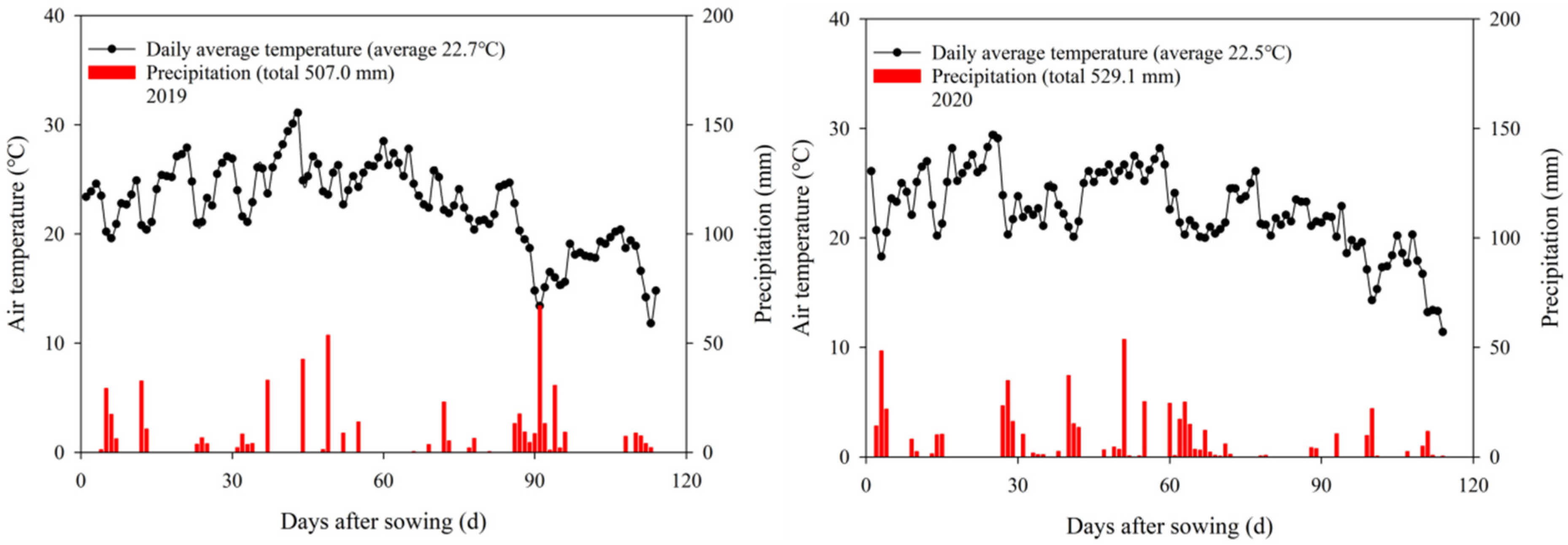
2.1. Experimental Site Description

Our analysis and modeling were implemented assuming performed typical production conditions, input usage and crop yield at the Key Laboratory of Agricultural Soil and Water Engineering (34°18′ N, 108°24′ E and 521 m ASL) in Arid and Semiarid Areas of the Ministry of Education for over two continuous growing seasons of 2019 and 2020. The site is located in a typical semi-humid and drought-prone region. Over the past 25 years (1995–2019), the average annual precipitation is 595 mm, with about 61% of total rainfall occurring between June and September. The average annual air temperature was 13.3 °C, soil evaporation was 1500 mm, sunshine was 2185 h and the duration of the frost-free period was more than 210 d in the test region, respectively. The daily average temperature, precipitation and sunshine hours during the growing seasons of soybeans in 2019 and 2020 are shown in Figure 1. The soil is loam and its main properties are listed in

Table 1. Basic soil properties of the 0–20 cm soil layer at the beginning of the experiment during the soybean growing seasons of 2019 and 2020.

Soil Properties	2019–2020	2020–2021
Organic matter (g kg−1)	12.50	14.30
Total nitrogen (g kg−1)	0.87	0.90
Nitrate nitrogen (mg kg−1)	76.30	82.30
Available phosphorus (mg kg−1)	23.30	25.30
Available potassium (mg kg−1)	133.80	145.70
pH (water)	8.10	8.00
Dry bulk density (g cm−3)	1.40	1.41
Field capacity (%)	24.00	23.90
Permanent wilting point (%)	8.50	8.50

.

2.2. Experimental Design and Field Management

Through the two-year field trials in 2019 and 2020, the yield distributions of eleven management alternatives and one conventional practice were considered. The experimental design was a re-split-plot design. The main plot was planting density (D₁: 160,000 plants ha⁻¹ and D₂: 320,000 plants ha⁻¹). The split plot was fertilization rate (F₁: 20 kg ha⁻¹ N, 30 kg ha⁻¹ P, 30 kg ha⁻¹ K; F₂: 40 kg ha⁻¹ N, 60 kg ha⁻¹ P, 60 kg ha⁻¹ K). The re-split plot was planting pattern, i.e., R+W₀: plastic-mulched ridge-furrow cultivation (PMRF) with no irrigation; R+W₁: PMRF with supplemental irrigation amount of 30 mm at the pod-filling stage; F+W₀: flat cultivation with no mulching (FTNM) with no irrigation. The detailed management combinations are shown in

Table 2. Re-split-plot design of test factors combinations.

Management Practice	Main Plot	Split Plot	Re-Split Plot
A	D1 (160,000 plants ha−1)	F1: 20 kg ha−1 N, 30 kg ha−1 P, 30 kg ha−1 K	R+W0
B			R+W1
C			F+W0
D		F2: 40 kg ha−1 N, 60 kg ha−1 P, 60 kg ha−1 K	R+W0
E			R+W1
F			F+W0
G	D2 (320,000 plants ha−1)	F1: 20 kg ha−1 N, 30 kg ha−1 P, 30 kg ha−1 K	R+W0
H			R+W1
I			F+W0
J		F2: 40 kg ha−1 N, 60 kg ha−1 P, 60 kg ha−1 K	R+W0
K			R+W1
L			F+W0

R+W₀: plastic-mulched ridge-furrow cultivation (PMRF) with no irrigation, R+W₁: PMRF with supplemental irrigation amount of 30 mm at the pod filling stage, F+W₀: flat cultivation with no mulching (FTNM) with no irrigation.

, where F is the local management practice. Fertilizers were applied before sowing, with the nitrogen fertilizer of urea (total nitrogen ≥ 46.0%, mass fraction, the same below), potassium fertilizer of potassium sulfate (K₂O ≥ 51.0%, Cl⁻ ≤ 1.5%) and phosphate fertilizer of superphosphate (P₂O₅ ≥ 16.0%). Summer soybean (Zhonghuang 37, bred by the Institute of Crop Science, Chinese Academy of Agricultural Sciences, Beijing, China) was planted on 15 June 2019 and harvested on 7 October 2019; the corresponding dates were 13 June and 5 October 2020. Soybean yields from field trials with 12 rainfed soybean production systems in northwest China over two years were used for subsequent analysis.

3. Economic Evaluation and Risk Premium Estimation

3.1. Economic Return and Production-to-Investment Ratio

This study considered economic return within the hypothetical range of price fluctuation and assumed that soybean production costs remain constant. The data on soybean price fluctuations were from market research data from multiple exchanges from January 2014 and June 2021 and were used for subsequent analysis. The average net income (NI_a), the minimum net income (NI_min) and the maximum net income (NI_max) were calculated. The economic return (Chinese Yuan (CNY) ha⁻¹) for each management practice was calculated by the following equations [25]:

$$\mathrm{OV}=\mathrm{GY}\times {\mathrm{P}}_{\mathrm{GY}}+\mathrm{SY}\times {\mathrm{P}}_{\mathrm{SY}}$$

(1)

$$\mathrm{IV}=\mathrm{FHPC}+\mathrm{SC}+\mathrm{PFC}+\mathrm{IWC}+\mathrm{MFC}+\mathrm{LC}$$

(2)

$$\mathrm{NI}=\mathrm{OV}-\mathrm{IV}$$

(3)

$$\mathrm{O}/\mathrm{I}=\frac{\mathrm{OV}}{\mathrm{IV}}$$

(4)

where OV: output, CNY ha⁻¹; GY and SY: grain yield and straw yield, Kg ha⁻¹, respectively; P_GY and P_SY: the grain price and straw price, CNY kg⁻¹, respectively; IV: input value, CNY ha⁻¹; FHPC: the costs of the fertilizers, herbicides and pesticide, CNY ha⁻¹; SC: seed costs, CNY ha⁻¹; PFC: plastic film costs, CNY ha⁻¹; IWC: irrigation water costs, CNY ha⁻¹; MFC: machinery use and fuel costs, CNY ha⁻¹; LC: labor costs, CNY ha⁻¹; NI: net income, CNY ha⁻¹; O/I: production-to-investment ratio.

3.2. Economic Analysis

The net present value method was used to calculate the economic evaluation of 12 production systems under three types of economic returns. An assumption was made that all the initial investment in the calculation of the NPV came from bank loans. NPV is the difference between the present value of future capital inflows and the present value of future capital flows [26]. The net present value is usually used in agricultural decision making, especially when making the first investment decision. The mathematical expression of the net present value was as follows [27]:

$$\mathrm{NPV}=-{\mathrm{C}}_0+{\displaystyle \sum _{\mathrm{t}=1}^{\mathrm{T}}\frac{{\mathrm{C}}_{\mathrm{t}}}{{(1+\mathrm{r})}^{\mathrm{t}}}}$$

(5)

where C₀ is the initial investment, in CNY; C_t is cash flow in year t, in CNY; r is the annual real interest rate or the discount rate; t is the time period, in years; NPV is net present value, in CNY.

The internal rate of return (IRR) is the rate of return used in the capital budget to measure and compare the profitability of investments. It is the ratio that produces NPV = 0 in a given period [28]. In addition, the payback period in the capital budget refers to the time required to recover the investment funds or reach the break-even point [29].

3.3. Economic Risk Analysis

The risk premium is a core concept of financial economics. It refers to investors’ demand for higher returns to offset greater risks. It is the compensation that investors demand for their own risks. Here, we made a hypothesis that all the investment in the estimation of risk premium came from personal investment. The stochastic dominance analysis with respect to a function (SDRF) and stochastic efficiency with respect to a function (SERF) ranks a set of risk alternatives according to the deterministic equivalence of a specific range of attitudes to risk. It can be used to determine the utility function of the risk attitude defined by the absolute, relative or partial risk aversion coefficient of the corresponding range [30]. SERF analysis uses effective alternatives for a range of risk attitudes, which considers the full range of decision-makers’ preferences. It is considered a more discriminatory and efficient method [31]. Compared with the traditional method of stochastic dominance analysis with respect to a function (SDRF), SERF includes simultaneous comparisons of each option and all other options, rather than pairwise comparisons. Therefore, within the same risk attitude, it can produce a smaller effective set than a simple paired SDRF. In addition, this method can be easily implemented.

Risk assessment often needs to grasp the possibility and preference of decision-makers for results. The chances of bad and good results can only be evaluated and compared by understanding the relative preferences of decision-makers for such results. According to the subjective expected utility (SEU) hypothesis, the utility function of the decision-maker on the outcome is necessary for evaluating risk alternatives, because the shape of the utility function reflects the individual’s attitude towards risk. The SEU hypothesis states that the utility of a risky alternative is the expected utility of the alternative, that is, the probability-weighted average of the utility of the result. Obviously, as a behavioral choice theory, the SEU hypothesis is flawed. Meyer et al. [32] believed that the SEU hypothesis was still the most suitable theory for prescriptive evaluation of risk choices. The utility function (U(w)) of decision-makers with w (wealth) as the performance standard. Evaluating the risk of a particular decision depends on the decision-maker’s degree of risk aversion to the potential utility function, which is to compare a function (SERF) with random efficiency and rank the risk alternatives in the form of alternative utility functions [33]. SERF estimates the deterministic equivalent of ranking a set of risk-effective alternatives in a series of risk aversion preferences. The fewer restrictions imposed on the utility function, the more general the applicability of the results, but the smaller the role of criteria when choosing a solution.

In this study, since we assumed that the 11 risk options to be compared had uncertain results, the value of w was random. Let f₁(w), f₂(w),…, f₁₁(w) be the probability density function describing the results of the 11 risk alternatives in this study. The corresponding cumulative distribution function was represented by F1(w), F2(w),…, F11(w). SEU assumed that the utility of any risk substitution was equal to its expected value as described in Equation (6) [30]:

$$\mathrm{U}(\mathrm{w})=\mathrm{EU}(\mathrm{w})={\displaystyle \int \mathrm{U}(\mathrm{w})\mathrm{f}(\mathrm{w})}\mathrm{dw}={\displaystyle \int \mathrm{U}\left(\mathrm{w}\right)}\mathrm{dF}\left(\mathrm{w}\right)$$

(6)

Because the utility function is an unknown and unfixed form [34], there are various function types, e.g., a constant absolute risk aversion negative exponential function, quadratic, exponent and a hyperbolic absolute risk aversion type utility function, constant relative risk aversion power function, parameterized restrictions to constant or decreasing absolute risk aversion expo-power function [35], and decreasing absolute risk aversion log utility function. Decision-makers who prefer more wealth rather than less wealth and have absolute risk aversion to wealth divide alternatives, where −∞ < r_a(w) < ∞, when the decision-maker is not inclined to risk, that is, 0 < r_a(w) < ∞. In practical applications, these two forms of analysis are not sufficiently distinguishable to produce useful results, which means that within a given range of risk aversion, the preferred alternative may still be too large and too much [36]. In other words, the decision-maker’s exact risk aversion is unspecified, so when the decision-maker’s absolute, relative or partial risk aversion function r(w) is limited to the upper and lower bounds r₁(w) and r₂(w), the problem is solved. Therefore, for each risk choice and a selected form of the utility function, the utility function in terms of risk aversion and random outcome w is defined as [30]:

$$\mathrm{U}\left(\mathrm{w}\right)={\displaystyle \int \mathrm{U}\left(\mathrm{w}\right)}\mathrm{dF}(\mathrm{w})\approx {\displaystyle \sum _{\mathrm{i}=1}^{\mathrm{m}}{\mathrm{U}(\mathrm{w}}_{\mathrm{i}},\mathrm{r}\left(\mathrm{w}\right))}{\mathrm{P}(\mathrm{w}}_{\mathrm{i}}),{\mathrm{r}}_1(\mathrm{w})\le \mathrm{r}(\mathrm{w})\le {\mathrm{r}}_2(\mathrm{w})$$

(7)

where the discrete case P(w_i) is the probability for states i and there are m states for each risky alternative in the discrete case.

SERF ranks the alternatives according to the deterministic equivalent (CE). The partial ordering of the alternatives by CE (CE with different values within the defined range) was the same as the partial ordering of them by the utility value [37], which is used as a selected measure of risk aversion. For more convenience, CE values were calculated using the following formula [30]:

$$\mathrm{CE}(\mathrm{w},\mathrm{r}(\mathrm{w}))={\mathrm{U}}^{-1}(\mathrm{w}, \mathrm{r}\left(\mathrm{w}\right))$$

(8)

The utility function in this study was the negative exponential function of absolute risk aversion (CARA). Negative exponential function can be used as a reasonable approximation of risk aversion behavior [38]; the equation was as follows and the estimated CE under CARA was defined as

$$\mathrm{U}(\mathrm{w})=-\exp (-{\mathrm{r}}_{\mathrm{a}}\mathrm{w})$$

(9)

$$\mathrm{CE}(\mathrm{w},{\mathrm{r}}_{\mathrm{a}}(\mathrm{w}))=\mathrm{In}\left\{\left.{\left(\frac{{\displaystyle \sum _{\mathrm{i}}^{\mathrm{n}}\exp (-{\mathrm{r}}_{\mathrm{a}}{\left(\mathrm{w}\right)\mathrm{w}}_{\mathrm{i}})}}{\mathrm{n}}\right)}^{-\frac{1}{{\mathrm{r}}_{\mathrm{a}}\left(\mathrm{w}\right)}}\right\}\right.$$

(10)

where r_a(w) represents absolute risk aversion coefficients (ARACs), and n is the number of alternatives.

The simplified method proposed by Hardaker et al. [30] is used to analyze the stochastic efficiency with the risk aversion bounds. The SERF method uses a utility function to estimate the CE values over a range of absolute risk aversion coefficients (ARAC). ARAC values were calculated using the following equation [24]:

$${\mathrm{ARAC}}_{\mathrm{w}}=\frac{{\mathrm{r}}_{\mathrm{r}}\left(\mathrm{w}\right)}{\mathrm{w}}$$

(11)

where r_r(w) is the relative risk aversion coefficient with respect to wealth (w), the value of r_r(w) is set from zero to four and risk aversion increases as r_r(w) value approach to four (neutral risk aversion r_r(w) = 0; average (normal) risk aversion r_r(w) = 1; rather clear risk aversion r_r(w) = 2; strong risk aversion r_r(w) = 3; very strong risk (extremely) aversion r_r(w) = 4), which were proposed by Anderson and Dillo [9]. Wealth (w) was calculated based on the average net return of the traditional farming planting mode and the other 11 planting alternatives.

4. Results and Discussion

4.1. Data and Simulation

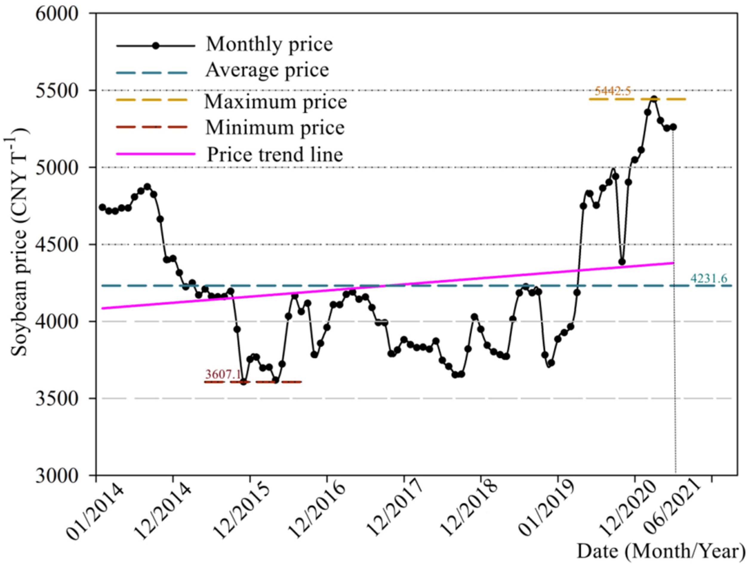
4.1.1. Fluctuating Prices of Soybean

Data on the fluctuating prices of soybeans was compiled from several sources for this partial budget analysis. Few studies have considered price fluctuations in the management of income risk; only Valvekar et al. [15] in the application of dairy cattle insurance involves the impact of milk price fluctuations in the past 20 years on economic analysis. According to the data of the Zhengzhou Commodity Exchange (ZCE), Shanghai Futures Exchange (SHFE), Dalian Commodity Exchange (DCE), China Financial Futures Exchange (CFFEX) and market research data in January 2014 and June 2021, the soybean monthly price volatility graph was obtained (Figure 2). Soybean prices showed an overall upward trend, and the average, maximum and minimum soybean prices were used to calculate NI_a, NI_min and NI_max, respectively. The existing problem was either insufficient funds or excessive funds, which may lead to inefficient natural resources management. Therefore, we assumed that the initial investment funds in the net present value (NPV) analysis came from bank loans, and the initial investment in the risk premium analysis came from personal investment.

4.1.2. Soybean Yield Analysis

Soybean production came from field surveys, using data from 2019–2020 to simulate the distribution of soybean production under 12 production systems (

Table 3. Summer soybean yields (kg ha⁻¹) under different production systems in 2019 and 2020.

Production Systems	Mean	St. Dev.	CV	Minimum	Maximum
A	3150.5	206.9	6.57%	2906.0	3439.2
B	3206.0	222.2	6.93%	2886.6	3458.7
C	2853.4	219.1	7.68%	2614.1	3085.6
D	3415.7	279.7	8.19%	3150.3	3742.6
E	3454.0	263.5	7.63%	3183.2	3791.8
F	3135.2	190.1	6.06%	2945.6	3414.8
G	3950.8	214.6	5.43%	3691.1	4307.2
H	3989.4	180.9	4.53%	3706.4	4124.1
I	3551.8	228.7	6.44%	3335.5	3845.6
J	4338.9	201.1	4.63%	4066.5	4590.1
K	4423.0	246.9	5.58%	4022.4	4695.9
L	3904.4	164.7	4.22%	3687.9	4103.2

). Compared to production system F (the planting system currently selected by most farmers), production system C (only reducing fertilization rate by half) decreased production by 8.99%; production system D (only considering replacing FTNM with PMRF) increased production by 8.95%; production system E (consider replacing FTNM with PMRF combined with supplemental irrigation during the critical period of soybean water demand) increased production by 10.17%; production system I (only reducing fertilization rate by half combined with double planting density) increased production by 13.29%; production system L (only double the planting density) increased production by 24.53%; all other production systems could achieve an increase in production, with the maximum increase of 66.04% in production system K (double planting density and replacing FTNM with PMRF combined with supplemental irrigation). The high-input approach may increase soybean production, but it also brings ecological and environmental issues [39]. A study evaluating soybean management in the U.S. Midwest also showed that high-input soybean should balance crop production and sustainability goals [40].

4.1.3. Input Costs of Soybean

Agriculture is a risk-prone activity, with many farmers operating under uncertain and risky conditions [8]. Preferences for different soybean planting systems depend on the return period and farmers’ attitudes towards risks, which are highly dependent on the initial investment and NI of the production system. Input costs included costs associated with fertilizer, herbicides, pesticides, seeds, plastic film, irrigation water, machinery use, fuel and operator labor. However, this study did not consider the impact of cost price volatility on economic analysis. Compared to production system F (

Table 4. Input costs under different production systems for summer soybean.

	Expense Item (CNY ha−1)	FHPC (CNY ha−1)	SC (CNY ha−1)	PFC (CNY ha−1)	IWC (CNY ha−1)	MFC (CNY ha−1)	LC (CNY ha−1)	IV (CNY ha−1)
Production Systems
A		1431.35	1732.50	803.92	0.00	2029.67	450.00	6447.44
B		1431.35	1732.50	803.92	120.00	2083.66	600.00	6771.43
C		1431.35	1732.50	0.00	0.00	1733.90	450.00	5347.75
D		2459.67	1732.50	803.92	0.00	2122.74	675.00	7793.83
E		2459.67	1732.50	803.92	120.00	2268.05	825.00	8209.14
F		2459.67	1732.50	0.00	0.00	1879.48	675.00	6746.65
G		1528.85	3465.00	1089.74	0.00	2511.77	750.00	9345.36
H		1528.85	3465.00	1089.74	120.00	2695.10	900.00	9798.69
I		1528.85	3465.00	0.00	0.00	2186.12	750.00	7929.96
J		2600.19	3465.00	1089.74	0.00	2667.34	975.00	10,797.27
K		2600.19	3465.00	1089.74	120.00	2802.24	1125.00	11,202.18
L		2600.19	3465.00	0.00	0.00	2324.94	975.00	9365.13

), production system C decreased costs by 20.73%; production system A (only reducing application rate by half combined with double planting density combined with replacing FTNM with PMRF) also decreased costs by 4.43%; production system D increased costs by 15.52%; production system E increased costs by 21.68%; production system I increased costs by 17.54%; production system L increased costs by 38.81%; and the other production systems also increased costs, with the maximum value of 66.04% in production system K.

4.1.4. Net Income of Soybean

Table 5. Summary statistics of simulated net income (CNY ha⁻¹) for summer soybean under different production systems.

Production Systems	Mean	St. Dev.	CV	Minimum	Maximum
A	7592.88	1684.32	22.18%	4705.64	12,783.04
B	7555.69	1767.98	23.40%	4266.70	12,774.65
C	7128.37	1544.33	21.66%	4556.73	11,899.56
D	7407.10	1888.32	25.49%	4284.87	13,270.30
E	7230.09	1889.81	26.14%	4074.28	13,229.71
F	7190.93	1627.47	22.63%	4498.81	12,426.98
G	8401.32	2048.71	24.39%	4985.11	15,117.28
H	8378.72	2065.40	24.65%	4666.09	14,594.08
I	8206.07	1882.86	22.94%	5141.01	13,999.36
J	8982.53	2208.50	24.59%	5170.27	15,537.08
K	8829.51	2287.72	25.91%	4621.10	15,690.02
L	8718.78	2095.96	24.04%	5214.48	15,539.96

lists the simulated economic returns of 12 soybean production systems under soybean price fluctuations. There was a big difference in NI of the each production system due to the fluctuation of soybean prices. Compared to production system F, production system C decreased NI by 0.87% because of less input costs and less yield; production system D increased NI by 3.01%; production system E increased NI by 0.54%; project I increased NI by 14.12%; production system L increased NI by 21.25%; production system A increased NI by 5.59% because of less input costs and high yield (by 0.49%); all other production systems also increased NI because of high output brought by high input costs and high yield; and production system J (replacing FTNM with PMRF combined with double planting density) obtained the a maximum increase of 24.91%.

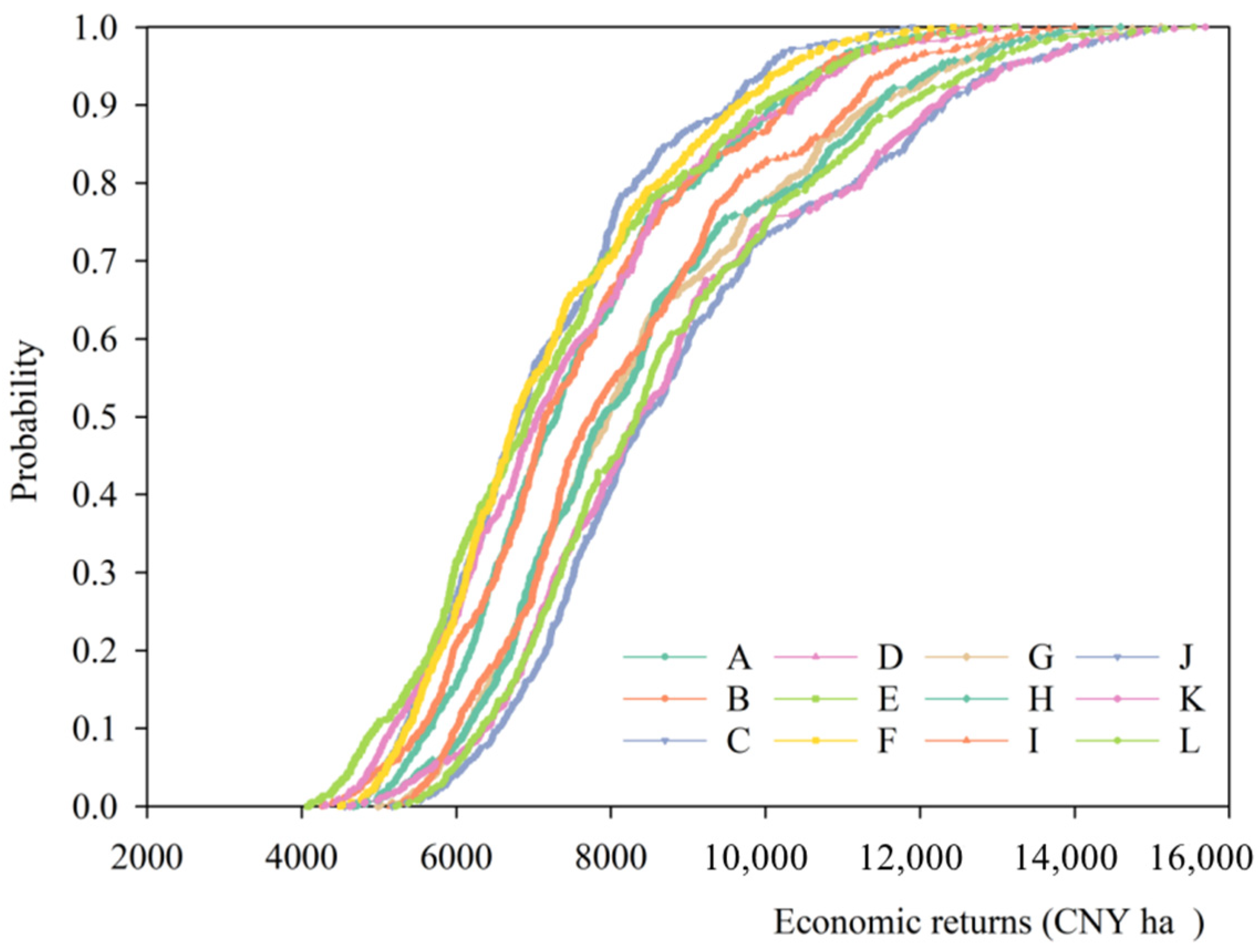
4.2. Economic Feasibility Analysis

Since summer soybean is an annual herbaceous crop, the investment period is one year. Most studies [27,41] are based on the average unit price for NPV analysis, but this study is different.

Table 6. NPV of the two investment periods in the three kinds of NI (CNY ha⁻¹).

Production Systems	IV	NIa	NImin	NImax	NPV1 at the Beginning of the First Year	NPV2 at the End of the First Year	NPV3 at the Beginning of the Second Year	NPV4 at the End of the Second Year (CNY)
A	6447.44	7592.88	4705.64	12,783.04	−IV	NI − i × IV	NI − (1 + i) × IV	(1) 2 × NI − i × IV, (CNY3 ≥ 0); (2) (2 + i) × NI − (2i + i2) × IV, (CNY3 < 0)
B	6771.43	7555.69	4266.7	12,774.65
C	5347.75	7128.37	4556.73	11,899.56
D	7793.83	7407.10	4284.87	13,270.3
E	8209.14	7230.09	4074.28	13,229.71
F	6746.65	7190.93	4498.81	12,426.98
G	9345.36	8401.32	4985.11	15,117.28
H	9798.69	8378.72	4666.09	14,594.08
I	7929.96	8206.07	5141.01	13,999.36
J	10,797.27	8982.53	5170.27	15,537.08
K	11,202.18	8829.51	4621.1	15,690.02
L	9365.13	8718.78	5214.48	15,539.96

calculates the NPV of the two investment periods under three kinds of NI. The initial funding comes from loans, so the investment of funds must consider the interest generated by the loan. Bank loansinterest is paid once a year, assuming that the annual interest rate of bank loans is i. According to the data of the People’s Bank of China (PBOC), the agricultural loan interest rate i ≤ 5%, and the annual net income refers to the results of economic analysis.

It can be seen from Table 6 that under NI_a, the payback period of production systems A, B, C and F was 1 year; that is, NPV₂ ≥ 0. The payback period of production systems D, E, G, H, J, K and L was 2 years; that is, NPV₂ < 0. When the agricultural loan interest rate i < 3.48%, the payback period of production system I was 1 year; when the agricultural loan interest rate was 3.48% ≤ i ≤ 5%, the payback period of production system I was 2 years; from a long-term perspective, choosing production system J would bring more economic returns (when i = 0, NPV₄ = 17,956 CNY ha⁻¹; when i = 5%, NPV₄ = 17,307.47 CNY ha⁻¹). Under the NI_min, the payback period of all production systems was 2 years; from a long-term perspective, choosing production system L will bring more economic returns (when i = 0, NPV₄ = 10,428 CNY ha⁻¹; when i = 5%, NPV₄ = 9729.76 CNY ha⁻¹). Under NI_max, the payback period of all production systems was 1 year; in the long run, choosing production system K would bring more economic returns (when i = 0, NPV₄ = 31,380 CNY ha⁻¹; when i = 5%, NPV₄ = 30,819.93 CNY ha⁻¹). Therefore, for farmers to make long-term investments through loans, choosing high-fertilizer and high-density production systems (production systems J, K and L) had higher economic returns. A similar conclusion also can be drawn from a study case in Pakistan [42]. From the perspective of the environmental protection department, it was hoped that farmers would reduce the use of nitrogen while increasing their income. Under the three kinds of NI, only production systems G, H and I had greater NPV₂ than production system F, but choosing production system G would bring greater returns (under NI_a, when i = 5%, NPV_4F = 14,044.53 CNY ha⁻¹, NPV_4G = 16,264.81 CNY ha⁻¹ under NI_a, increased NI by 15.81%; NPV_4F = 8531.03 CNY ha⁻¹, NPV_4G = 9726.25 CNY ha⁻¹ under NI_min, increased NI by 14.01%; NPV_4F = 24,516.63 CNY ha⁻¹, NPV_4G = 29,767.292 CNY ha⁻¹ under NI_max, increased NI by 21.42%). All the other production systems were not satisfied even if the interest rate was 0; therefore, the environmental protection department should strongly recommend that the farmers who have passed the loan choose production system G.

4.3. Risk Premium Estimation

A cumulative distribution function of hypothetical economic returns is shown in Figure 3. Each production system contained 540 values sufficient to evaluate the distribution hypothesis. We assumed that the realistic upper limit r_r(w) of relative risk aversion was 4. According to the average economic returns level (w) of the 12 production systems, the wealth exponent parameter for the expo-power function was set at 0~0.052. As shown in Figure 4, the SERF method provided a figure to explain the ranking of risky production systems by different farmers. It can be clearly found from Figure 3 that for a specific level of risk aversion, a subset of the effective SERF set can be formed. Therefore, for farmers whose absolute risk aversion level was less than 0.0223, the SERF effective set contained only production system J; for decision-makers whose risk aversion level was greater than 0.0223 and less than 0.0321, it only contained production system K; and for farmers whose absolute risk aversion level was greater than 0.0321, it only contained production system L.

When dealing with farmers with different levels of risk tolerance, it was important to consider their risky behaviors and determine the level of incentives that encourage the adoption of protective practices. For the purpose of discussion, it is proposed to transfer from production system F to other production systems. The data in

Table 7. Certainty equivalents and risk premiums for various absolute risk aversion coefficients.

	Absolute Risk Aversion Coefficient (ARAC)
	0.000	0.013	0.026	0.039	0.052
Production systems	Certainty Equivalents (CNY ha−1)
A	7592.88	7418.43	7262.73	7124.30	7001.13
B	7555.69	7362.83	7189.39	7033.80	6893.91
C	7128.37	6981.18	6848.66	6729.79	6623.19
D	7407.10	7189.15	6997.01	6828.21	6679.74
E	7230.09	7011.46	6818.13	6647.73	6497.26
F	7190.93	7028.32	6883.72	6755.74	6642.47
G	8401.32	8147.49	7929.05	7741.86	7580.91
H	8378.72	8119.70	7895.01	7700.80	7532.06
I	8206.07	7989.72	7799.87	7634.04	7488.99
J	8982.53	8575.59	8218.44	7904.20	7624.95
K	8829.51	8513.23	8241.66	8008.86	7807.52
L	8718.78	8452.97	8223.86	8027.08	7857.44
Risk premiums (CNY ha−1)
A	401.95	390.11	379.01	368.56	358.65
B	364.76	334.51	305.67	278.06	251.44
C	−62.55	−47.14	−35.06	−25.95	−19.29
D	216.17	160.83	113.28	72.47	37.26
E	39.17	−16.86	−65.59	−108.02	−145.21
F	0.00	0.00	0.00	0.00	0.00
G	1210.39	1119.17	1045.32	986.12	938.43
H	1187.80	1091.37	1011.28	945.06	889.59
I	1015.14	961.40	916.15	878.30	846.51
J	1791.61	1547.27	1334.71	1148.46	982.48
K	1638.58	1484.91	1357.94	1253.12	1165.04
L	1527.86	1424.65	1340.13	1271.34	1214.96

shows that if farmers change their soil production systems and crop production systems, they may still increase economic benefits. For farmers with neutral risk aversion (ARAC = 0.000) and normal risk aversion (ARAC = 0.013) who changed the production system from F to J could increase their NI most, which were 1791.61 CNY ha⁻¹ and 1547.27 CNY ha⁻¹, respectively. For farmers with rather clear risk aversion (ARAC = 0.026), change the production system to K but their net income will increase by at least 1357.94 CNY ha⁻¹. For farmers with strong risk aversion (ARAC = 0.039) and very strong (extremely) risk aversion (ARAC = 0.052), production system L would bring them the largest net income of 1271.34 CNY ha⁻¹ and 1214.96 CNY ha⁻¹, respectively. Greenhouse gas (GHG) emissions were closely related to the amount of chemical fertilizers used, and the increase in GHG emissions leads to climate change with shifting weather patterns and serious ecological imbalances [43]. From the perspective of the environmental protection department, if farmers (take farmers with neutral risk aversion as an example) were to be persuaded to reduce the use of fertilizers (such as changing the production system from F to C), the farmers would need 1133.90 CNY ha⁻¹ to continue the current production system, or the environmental protection department was willing to pay 62.55 CNY ha⁻¹ (7190.93 CNY ha⁻¹~7128.37 CNY ha⁻¹ as the difference in CE values under that ARAC value) to persuade farmers to move production system F to production system C, because NI was higher under production system F; the research of Adusumilli et al. [31] has a similar approach. The environmental protection department could recommend that farmers choose production systems A or B to increase income and reduce the use of fertilizers. Production system B needed to slightly increase input costs, but production system A could reduce the input costs. Although the production system of increasing planting density combined with reducing fertilizer application can also achieve the goal of reducing nitrogen rate and increasing income, it also greatly increases the input costs at the same time. Therefore, the environmental protection department should vigorously promote production system A. Water deficit will have a serious impact on soybean yield [44], but it can be seen from Table 7 that the NI of the production system that PMRF combined with supplemental irrigation during the critical period of soybean water demand was always lower than the production system that of only the PMRF. This may be because PMRF itself inhibited evaporation and collected rainfall to make production systems that PMRF combined with supplemental irrigation during the critical period of soybean water demand did not increase the yield significantly. More importantly, it also increased irrigation costs, and the increased costs of supplemental irrigation nullify the returns attributable to increased yield. In other words, the production system that PMRF combined with supplemental irrigation during the critical period of soybean water demand was an uneconomical and unwise behavior, and irrigation should not be carried out under non-essential conditions.

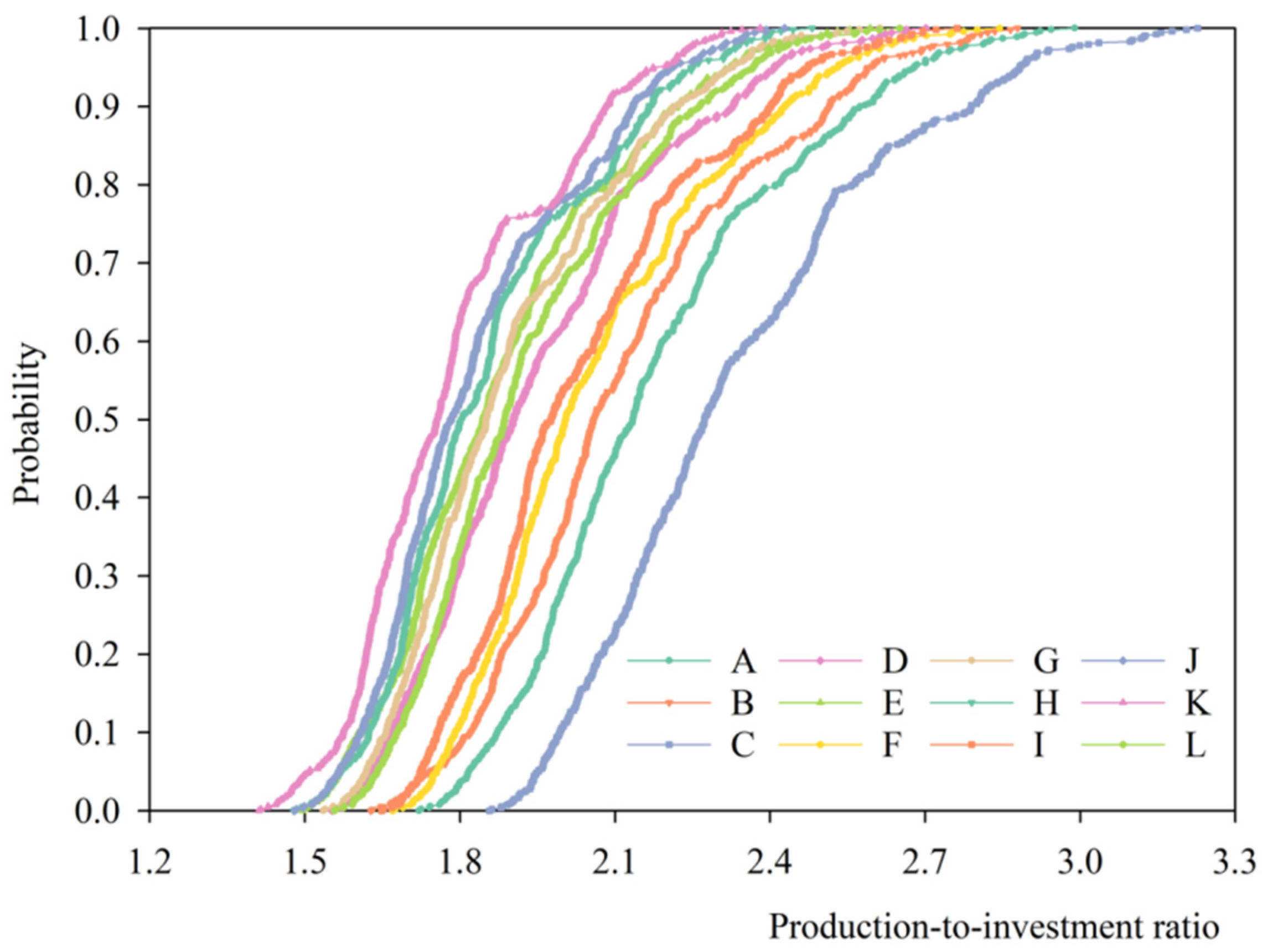
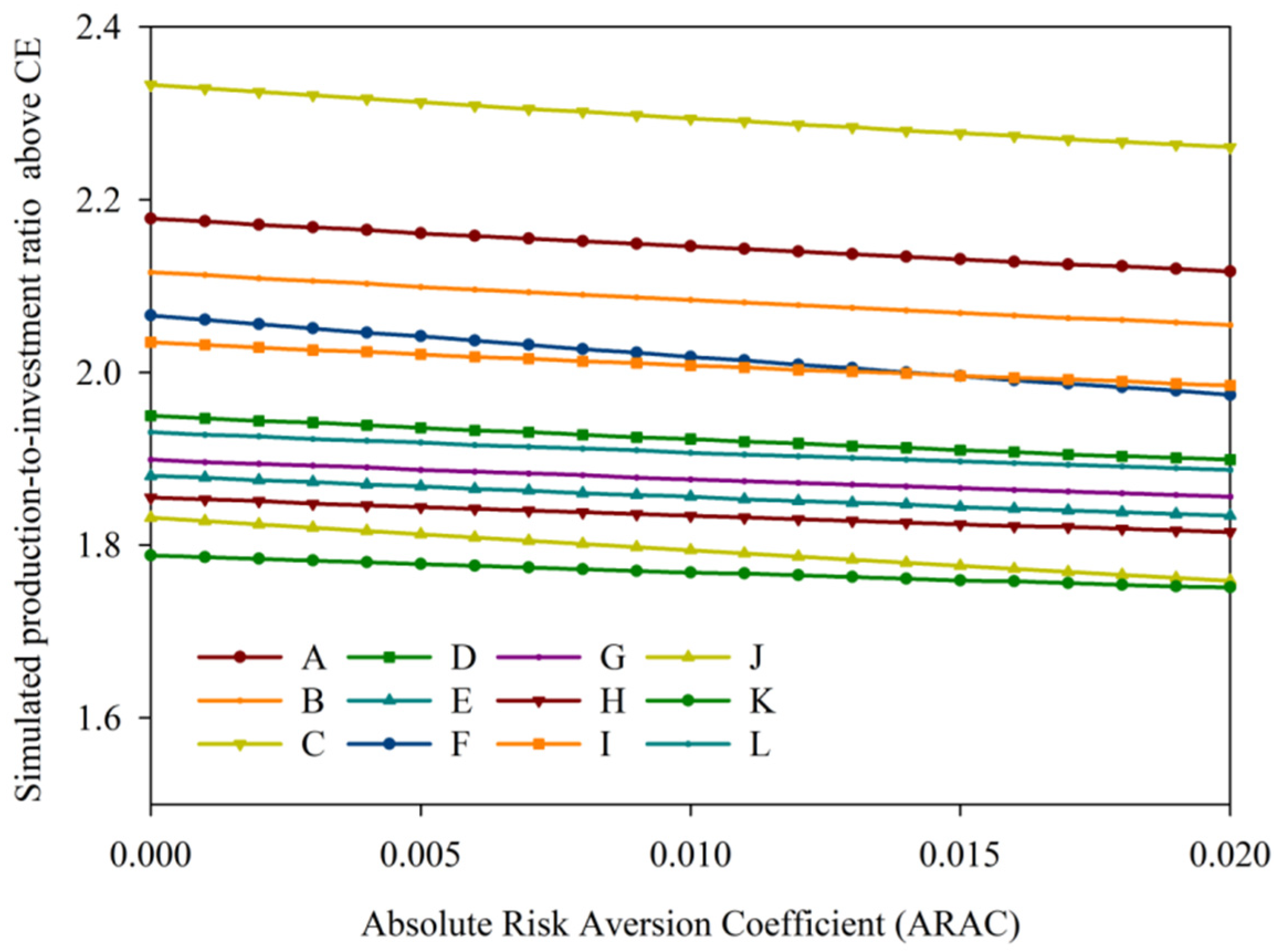
4.4. Estimation of Production-to-Investment Ratio

Farmers’ attitudes towards risks are directly reflected in economic benefits [24], while previous studies have hardly involved the production-to-investment ratio (O/I). From the previous analysis in this study, it can be seen that the reasons for the increase in NI and the magnitude of the increase in NI were not the same, so it is necessary to introduce the indicator of the O/I. From the perspective of O/I, higher O/I meant a higher cost–performance ratio. With reference to the calculation method of the risk premium, we also used the stochastic efficiency method to estimate the O/I overflow under different production systems. It can be seen from

Table 8. Summary statistics of simulated production-to-investment ratio for summer soybean planting patterns.

Production Systems	Mean	St. Dev.	CV	Minimum	Maximum
A	2.178	0.264	12.11%	1.721	2.990
B	2.116	0.262	12.37%	1.628	2.879
C	2.333	0.290	12.41%	1.857	3.227
D	1.950	0.241	12.38%	1.552	2.702
E	1.880	0.228	12.14%	1.496	2.594
F	2.066	0.242	11.70%	1.670	2.845
G	1.899	0.219	11.52%	1.536	2.613
H	1.855	0.210	11.34%	1.478	2.482
I	2.035	0.236	11.62%	1.648	2.763
J	1.832	0.204	11.12%	1.480	2.429
K	1.788	0.203	11.34%	1.411	2.382
L	1.931	0.222	11.52%	1.557	2.651

that the O/I of each production system was greater than 1; that is, NI > 0, so that NPV > 0, indicating that each production system was economically feasible. Among all the production systems, the production systems of reducing fertilization rate by half (production systems A, B, C) had higher O/I, among which production system C had the highest cost performance. Except for these three production systems, the O/I of other production systems was lower than that of production system F, which also explained why most farmers chose production system F in the past. Compared with production system F, choosing high-fertilizer combined with high-density production systems (production systems J, K, L) reduced the O/I by 6.53~13.46%.

From the cumulative distribution function of the assumed O/I (Figure 5) and the SERF results of production systems for summer soybean O/I above CE (Figure 6), it can be seen that farmers with different levels of risk aversion should choose production system C in order to pursue the highest cost performance. A study also showed that when dealing with various risks, most farmers prefer to choose highest cost performance alternatives [45].

In order to pursue higher cost performance, as shown in

Table 9. Certainty equivalents and production-to-investment ratio for various absolute risk aversion coefficients.

	Absolute Risk Aversion Coefficient (ARAC)
	0.000	0.005	0.010	0.015	0.020
Production Systems	Certainty Equivalents
A	2.178	2.161	2.146	2.131	2.117
B	2.116	2.099	2.084	2.069	2.055
C	2.333	2.313	2.294	2.277	2.261
D	1.950	1.936	1.923	1.910	1.899
E	1.880	1.868	1.856	1.844	1.834
F	2.066	2.042	2.018	1.996	1.974
G	1.899	1.887	1.876	1.866	1.856
H	1.855	1.844	1.834	1.824	1.815
I	2.035	2.021	2.008	1.996	1.985
J	1.832	1.813	1.794	1.776	1.759
K	1.788	1.778	1.768	1.759	1.751
L	1.931	1.919	1.907	1.897	1.887
Production-to-investment ratio spillover
A	0.112	0.120	0.127	0.135	0.143
B	0.050	0.058	0.065	0.073	0.081
C	0.267	0.271	0.276	0.281	0.286
D	−0.116	−0.106	−0.095	−0.086	−0.076
E	−0.186	−0.174	−0.163	−0.151	−0.141
F	0.000	0.000	0.000	0.000	0.000
G	−0.167	−0.154	−0.142	−0.130	−0.118
H	−0.211	−0.197	−0.184	−0.171	−0.159
I	−0.031	−0.021	−0.010	0.001	0.011
J	−0.234	−0.229	−0.224	−0.220	−0.216
K	−0.278	−0.264	−0.250	−0.236	−0.224
L	−0.135	−0.123	−0.111	−0.099	−0.088

, farmers with neutral risk aversion (ARAC = 0.000), normal risk aversion (ARAC = 0.005) and rather clear risk aversion (ARAC = 0.010) can only choose production systems A, B and C. However, farmers with strong risk aversion (ARAC = 0.015) and very strong (extremely) risk aversion (ARAC = 0.020) can also choose production system I. Compared with production system F, their production-to-investment ratio spillover was 0.001 and 0.011, respectively. As Sulewski et al. [36] noticed, farmers’ attitude towards risk is substantial in making decisions; hence, it is desirable to consider making decisions that include not only risk premiums but also production-to-investment ratio spillover.

5. Conclusions

This study used the NPV method and the stochastic efficiency method to evaluate the profitability and risk premium of 12 soybean production systems in a semi-humid and drought-prone region of northwest China. We also aimed to provide an alternative rainfed soybean production system from the perspective of farmers and the environmental protection department in northwest China. The main conclusions were as follows. (1) For farmers with long-term investments through bank loans, high-fertilizer combined with high-density production systems obtained the highest economic benefit, but the production-to-investment ratio was reduced by 6.53~13.46%. From the perspective of the environmental protection department, they should recommend farmers choose production system G (reducing fertilizer application by half while increasing NI by 14.01~21.42%). (2) In the risk premium analysis based on personal investment, farmers with neutral and normal risk aversion should choose production system J; farmers with rather clear risk aversion should choose production system K; farmers with strong risk aversion and farmers with very strong risk aversion should choose production system L. From the perspective of the environmental protection department, they should recommend production system A (reducing fertilizer application by half while increasing production by 0.49%, reducing input costs by 4.43% and increasing NI by 5.54% with relatively high O/I) to farmers in this circumstance. (3) If the farmer pursues the greatest cost-effectiveness, the farmer’s first choice is production system C and production system A. These economic evaluations and economic analyses in this study will help farmers and government departments to provide protective alternatives and decision-making information from different perspectives.

References

1. FAOSTAT. ProdStat. Core Production Data Base, Electronic Resource. 2020. Available online: http://faostat.fao.org/ (accessed on 23 January 2020).
2. World Bank. Weather Index Insurance for Agriculture: Guidance for Development Practitioners; World Bank: Washington, DC, USA, 2011. [Google Scholar]
3. Júnior RS, N.; Sentelhas, P.C. Soybean-maize succession in Brazil: Impacts of sowing dates on climate variability, yields and economic profitability. Eur. J. Agron. 2019, 103, 140–151. [Google Scholar] [CrossRef]
4. Liao, Z.Q.; Zeng, H.L.; Fan, J.L.; Lai, Z.; Zhang, C.; Zhang, F.; Wang, H.; Cheng, M.; Guo, J.; Li, Z.; et al. Effects of plant density, nitrogen rate and supplemental irrigation on photosynthesis, root growth, seed yield and water-nitrogen use efficiency of soybean under ridge-furrow plastic mulching. Agric. Water Manag. 2022, 268, 107688. [Google Scholar] [CrossRef]
5. Chen, S.; Chen, X.; Xu, J. Impacts of climate change on agriculture: Evidence from China. J. Environ. Econ. Manag. 2016, 76, 105–124. [Google Scholar] [CrossRef]
6. Elahi, E.; Khalid, Z.; Tauni, M.Z.; Zhang, H.; Lirong, X. Extreme weather events risk to crop-production and the adaptation of innovative management strategies to mitigate the risk: A retrospective survey of rural Punjab, Pakistan. Technovation 2021, 117, 102255. [Google Scholar] [CrossRef]
7. Li, R.; Hou, X.; Jia, Z.; Han, Q. Soil environment and maize productivity in semi-humid regions prone to drought of Weibei Highland are improved by ridge-and-furrow tillage with mulching. Soil Tillage Res. 2020, 196, 104476. [Google Scholar] [CrossRef]
8. Akhtar, S.; Li, G.C.; Ullah, R.; Nazir, A.; Amjed, M.; Haseeb, M.; Iqbal, N.; Faisal, M. Factors influencing hybrid maize farmers’ risk attitudes and their perceptions in Punjab Province, Pakistan. J. Integr. Agric. 2018, 17, 1454–1462. [Google Scholar] [CrossRef]
9. Anderson, J.R.; Dillon, J.L. Risk Analysis in Dryland Farming Systems (No. 2); Food and Agriculture Organization: Rome, Italy, 1992. [Google Scholar]
10. Groom, B.; Koundouri, P.; Nauges, C.; Thomas, A. The story of the moment: Risk averse cypriot farmers respond to drought management. Appl. Econ. 2008, 40, 315–326. [Google Scholar] [CrossRef]
11. Gaspar, A.P.; Mitchell, P.D.; Conley, S.P. Economic risk and profitability of soybean fungicide and insecticide seed treatments at reduced seeding rates. Crop Sci. 2015, 55, 924–933. [Google Scholar] [CrossRef]
12. Gaspar, A.P.; Mueller, D.S.; Wise, K.A.; Chilvers, M.I.; Tenuta, A.U.; Conley, S.P. Response of Broad-Spectrum and Target-Specific Seed Treatments and Seeding Rate on Soybean Seed Yield, Profitability, and Economic Risk. Crop Sci. 2017, 57, 2251–2262. [Google Scholar] [CrossRef]
13. Babcock, B.A.; Choi, E.K.; Feinerman, E. Risk and probability premiums for CARA utility functions. J. Agric. Resour. Econ. 1993, 18, 17–24. [Google Scholar]
14. Boyer, C.N.; Stefanini, M.; Larson, J.A.; Smith, S.A.; Mengistu, A.; Bellaloui, N. Profitability and risk analysis of soybean planting date by maturity group. Agron. J. 2015, 107, 2253–2262. [Google Scholar] [CrossRef]
15. Valvekar, M.; Chavas, J.P.; Gould, B.W.; Cabrera, V.E. Revenue risk management, risk aversion and the use of livestock gross margin for dairy cattle insurance. Agric. Syst. 2011, 104, 671–678. [Google Scholar] [CrossRef]
16. Cormos, A.M.; Cormos, C.C. Techno-economic evaluations of post-combustion CO2 capture from sub-and super-critical circulated fluidised bed combustion (CFBC) power plants. Appl. Therm. Eng. 2017, 127, 106–115. [Google Scholar] [CrossRef]
17. Gwak, Y.R.; Kim, Y.B.; Gwak, I.S.; Lee, S.H. Economic evaluation of synthetic ethanol production by using domestic biowastes and coal mixture. Fuel 2018, 213, 115–122. [Google Scholar] [CrossRef]
18. Purola, T.; Lehtonen, H. Evaluating profitability of soil-renovation investments under crop rotation constraints in Finland. Agric. Syst. 2020, 180, 102762. [Google Scholar] [CrossRef]
19. Cavalett, O.; Ortega, E. Emergy, nutrients balance, and economic assessment of soybean production and industrialization in Brazil. J. Clean. Prod. 2009, 17, 762–771. [Google Scholar] [CrossRef]
20. Adler, P.R.; Hums, M.E.; McNeal, F.M.; Spatari, S. Evaluation of environmental and cost tradeoffs of producing energy from soybeans for on-farm use. J. Clean. Prod. 2019, 210, 1635–1649. [Google Scholar] [CrossRef]
21. Kamali, F.P.; Borges, J.A.R.; Meuwissen, M.P.M.; De Boer, I.J.M.; Oude Lansink, A.G.J.M. Sustainability assessment of agricultural systems: The validity of expert opinion and robustness of a multi-criteria analysis. Agric. Syst. 2017, 157, 118–128. [Google Scholar] [CrossRef]
22. Adusumilli, N.; Wang, H. Analysis of soil management and water conservation practices adoption among crop and pasture farmers in humid-south of the United States. Int. Soil Water Conserv. Res. 2018, 6, 79–86. [Google Scholar] [CrossRef]
23. Adusumilli, N.; Wang, H. Conservation adoption among owners and tenant farmers in the Southern United States. Agriculture 2019, 9, 53. [Google Scholar] [CrossRef]
24. Wang, H.; Adusumilli, N.; Gentry, D.; Fultz, L. Economic and stochastic efficiency analysis of alternative cover crop systems in Louisiana. Exp. Agric. 2020, 56, 651–661. [Google Scholar] [CrossRef]
25. Gang, X.; Huabing, L.; Yufu, P.; Tiezhao, Y.; Xi, Y.; Shixiao, X. Plastic film mulching combined with nutrient management to improve water use efficiency, production of rain-fed maize and economic returns in semi-arid regions. Field Crops Res. 2019, 231, 30–39. [Google Scholar] [CrossRef]
26. Lee, S.H.; Lee, T.H.; Jeong, S.M.; Lee, J.M. Economic analysis of a 600 mwe ultra supercritical circulating fluidized bed power plant based on coal tax and biomass co-combustion plans. Renew. Energy 2019, 138, 121–127. [Google Scholar] [CrossRef]
27. Adusumilli, N.; Davis, S.; Fromme, D. Economic evaluation of using surge valves in furrow irrigation of row crops in Louisiana: A net present value approach. Agric. Water Manag. 2016, 174, 61–65. [Google Scholar] [CrossRef]
28. Hernandez-Torres, D.; Bridier, L.; David, M.; Lauret, P.; Ardiale, T. Technico-economical analysis of a hybrid wave power-air compression storage system. Renew. Energy 2015, 74, 708–717. [Google Scholar] [CrossRef]
29. Gwak, I.S.; Hwang, J.H.; Sohn, J.M.; Lee, S.H. Economic evaluation of domestic biowaste to ethanol via a fluidized bed gasifier. J. Ind. Eng. Chem. 2017, 47, 391–398. [Google Scholar] [CrossRef]
30. Hardaker, J.B.; Richardson, J.W.; Lien, G.; Schumann, K.D. Stochastic efficiency analysis with risk aversion bounds: A simplified approach. Aust. J. Agric. Resour. Econ. 2004, 48, 253–270. [Google Scholar] [CrossRef]
31. Adusumilli, N.; Wang, H.; Dodla, S.; Deliberto, M. Estimating risk premiums for adopting no-till and cover crops production systems in soybean production system using stochastic efficiency approach. Agric. Syst. 2020, 178, 102744. [Google Scholar] [CrossRef]
32. Meyer, J. Expected utility as a paradigm for decision making in agriculture. In A Comprehensive Assessment of the Role of Risk in US Agriculture; Springer: Boston, MA, USA, 2002; pp. 3–19. [Google Scholar]
33. Schumann, K.D.; Richardson, J.W.; Lien, G.D.; Hardaker, J.B. Stochastic Efficiency Analysis Using Multiple Utility Functions. In Proceedings of the Association Annual Meeting, Denver, CO, USA, 1–4 August 2004. [Google Scholar]
34. Abdulkadri, A.O. Estimating risk aversion coefficients for dry land wheat, irrigated corn and dairy producers in Kansas. Appl. Econ. 2003, 35, 825–834. [Google Scholar] [CrossRef]
35. Saha, A. Expo-power utility: A ‘flexible’form for absolute and relative risk aversion. Am. J. Agric. Econ. 1993, 75, 905–913. [Google Scholar] [CrossRef]
36. Sulewski, P.; Wąs, A.; Kobus, P.; Pogodzińska, K.; Szymańska, M.; Sosulski, T. Farmers’ Attitudes towards Risk—An Empirical Study from Poland. Agronomy 2020, 10, 1555. [Google Scholar] [CrossRef]
37. Watkins, K.B.; Hill, J.L.; Anders, M.M. An economic risk analysis of no-till management and rental arrangements in Arkansas rice production. J. Soil Water Conserv. 2008, 63, 242–250. [Google Scholar] [CrossRef]
38. Williams, J.R.; Llewelyn, R.V.; Pendell, D.L.; Schlegel, A.; Dumler, T. A Risk Analysis of Converting Conservation Reserve Program Acres to a Wheat-Sorghum-Fallow Rotation. Agron. J. 2010, 102, 612–622. [Google Scholar] [CrossRef]
39. Van der Werf, H.M.G.; Knudsen, M.T.; Cederberg, C. Towards better representation of organic agriculture in life cycle assessment. Nat. Sustain. 2020, 3, 419–425. [Google Scholar] [CrossRef]
40. Greer, K.; Martins, C.; White, M.; Pittelkow, C.M. Assessment of high-input soybean management in the US Midwest: Balancing crop production with environmental performance. Agric. Ecosyst. Environ. 2020, 292, 106811. [Google Scholar] [CrossRef]
41. Boyer, C.N.; Lambert, D.M.; Larson, J.A.; Tyler, D.D. Investment analysis of cover crop and no-tillage systems on Tennessee cotton. Agron. J. 2018, 110, 331–338. [Google Scholar] [CrossRef]
42. Razzaq, A.; Xiao, M.; Zhou, Y.; Liu, H.; Abbas, A.; Liang, W.; Naseer, M.A.U.R. Impact of Participation in Groundwater Market on Farmland, Income and Water Access: Evidence from Pakistan. Water 2022, 14, 1832. [Google Scholar] [CrossRef]
43. Shi, Y.; Huang, G.; An, C.; Zhou, Y.; Yin, J. Assessment of regional greenhouse gas emissions from spring wheat cropping system: A case study of Saskatchewan in Canada. J. Clean. Prod. 2021, 301, 126917. [Google Scholar] [CrossRef]
44. Battisti, R.; Ferreira MD, P.; Tavares, É.B.; Knapp, F.M.; Bender, F.D.; Casaroli, D.; Júnior, J.A. Rules for grown soybean-maize cropping system in midwestern Brazil: Food production and economic profits. Agric. Syst. 2020, 182, 102850. [Google Scholar] [CrossRef]
45. Yang, G.T.; Li, J.; Liu, Z.; Zhang, Y.; Xu, X.; Zhang, H.; Xu, Y. Research trends in crop-livestock systems: A bibliometric review. Int. J. Environ. Res. Public Health 2022, 19, 8563. [Google Scholar] [CrossRef]
Figure 1. Daily air temperature and precipitation during the two growing seasons of summer soybean in 2019 and 2020.
Agronomy 13 02840 g001
Figure 2. Summer soybean monthly price volatility charts from January 2014 and June 2021. (CNY T−1: Chinese Yuan per ton.)
Agronomy 13 02840 g002
Figure 3. Cumulative distribution function for production systems A to L of hypothetical economic returns for SERF analysis.
Agronomy 13 02840 g003
Figure 4. SERF results of production systems for summer soybean simulated net returns (CE) over absolute risk aversion range of 0.000 to 0.052 assuming negative exponential utility function.
Agronomy 13 02840 g004
Figure 5. Cumulative distribution function for alternatives A to L of hypothetical production-to-investment ratio for SERF analysis.
Agronomy 13 02840 g005
Figure 6. SERF results of production systems for summer soybean production-to-investment ratio above CE over absolute risk aversion range of 0.000 to 0.020 assuming negative exponential utility function.
Agronomy 13 02840 g006