

What Affects the Corporate Performance of Listed Companies in China’s Agriculture and Forestry Industry?


Abstract
1. Introduction
2. Data and Methodology
2.1. Data Sources
2.2. Methodology
2.3. Variables
2.3.1. Indicator Selection
2.3.2. Variable Relationships
2.3.3. Entropy Weighting Method
2.4. Smoothing Tests
3. Empirical Analysis
3.1. PVAR Model Construction
3.2. PVAR Model Results
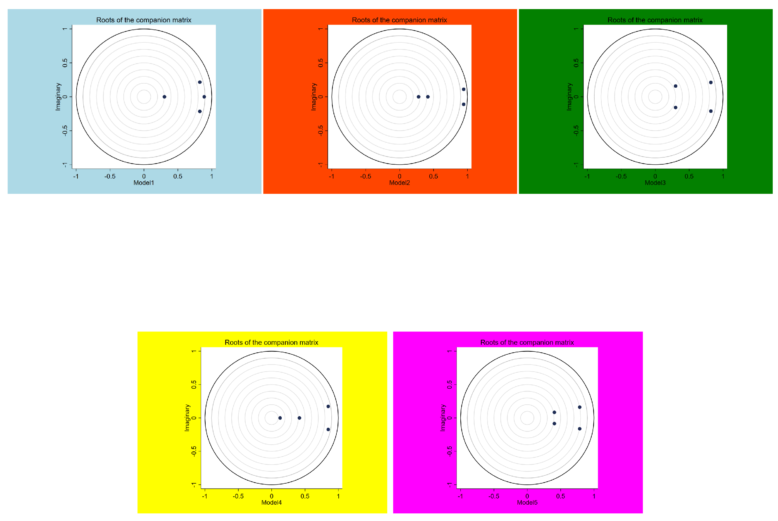
3.3. Robustness Tests
3.4. Granger Causality Test
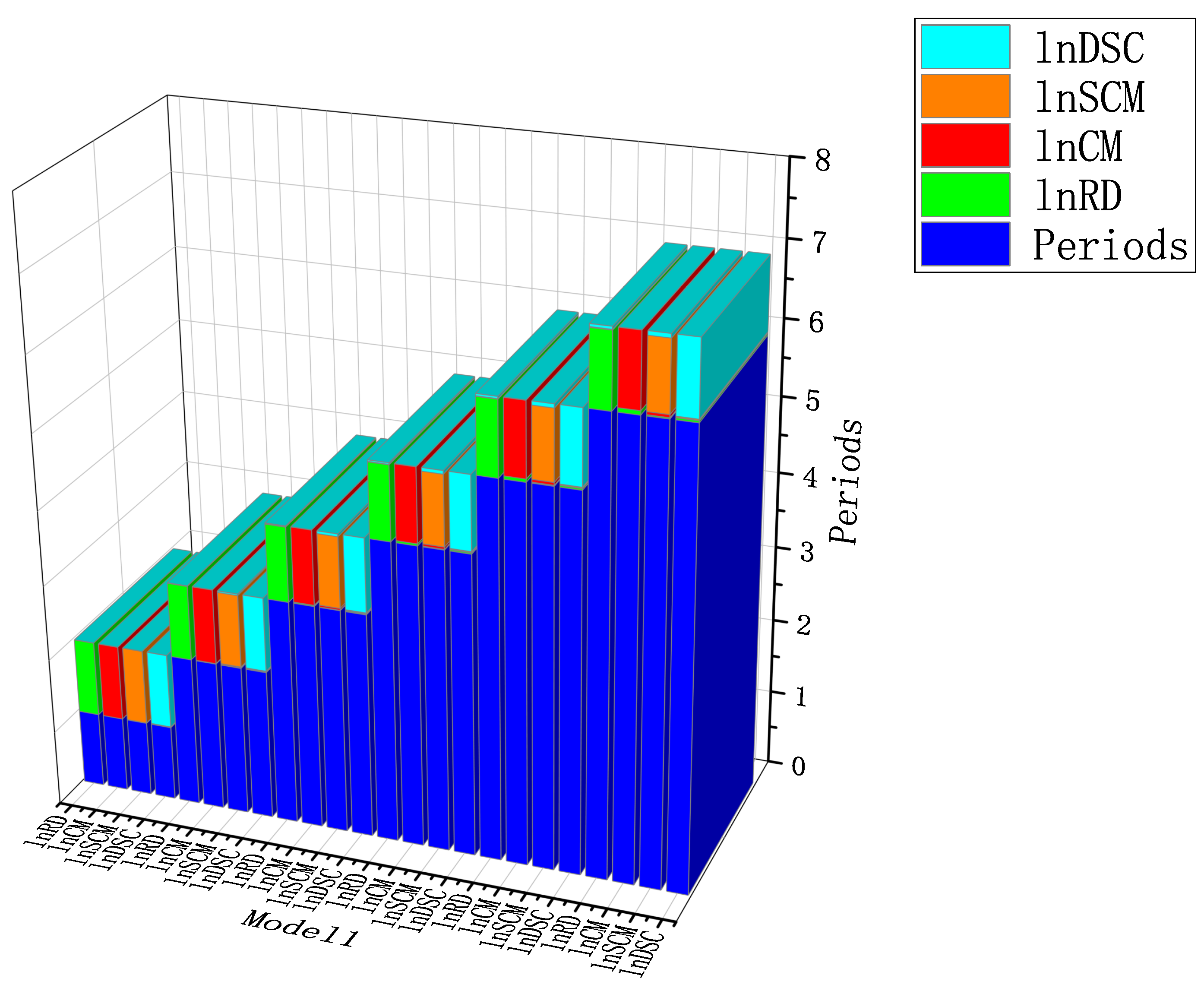
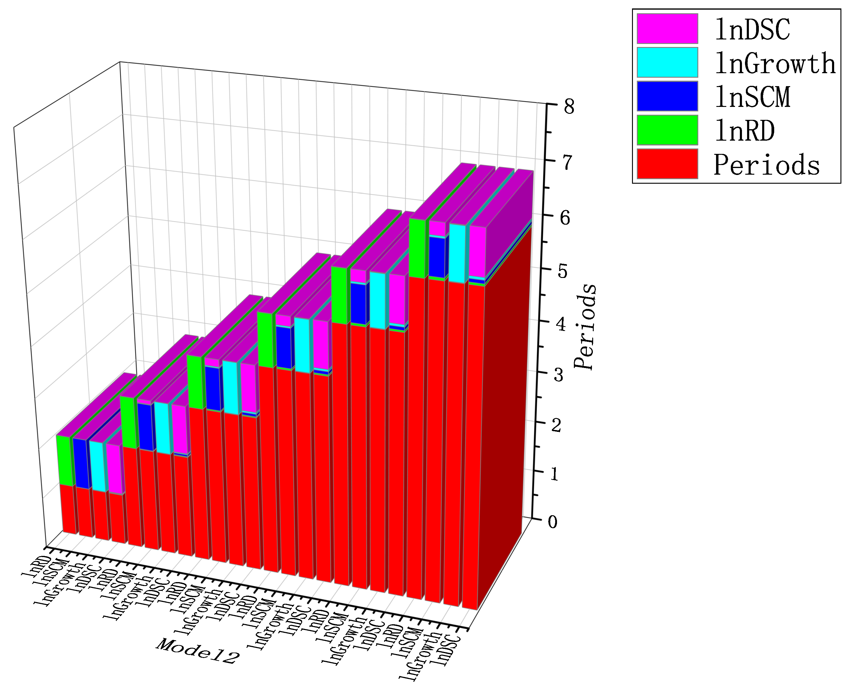
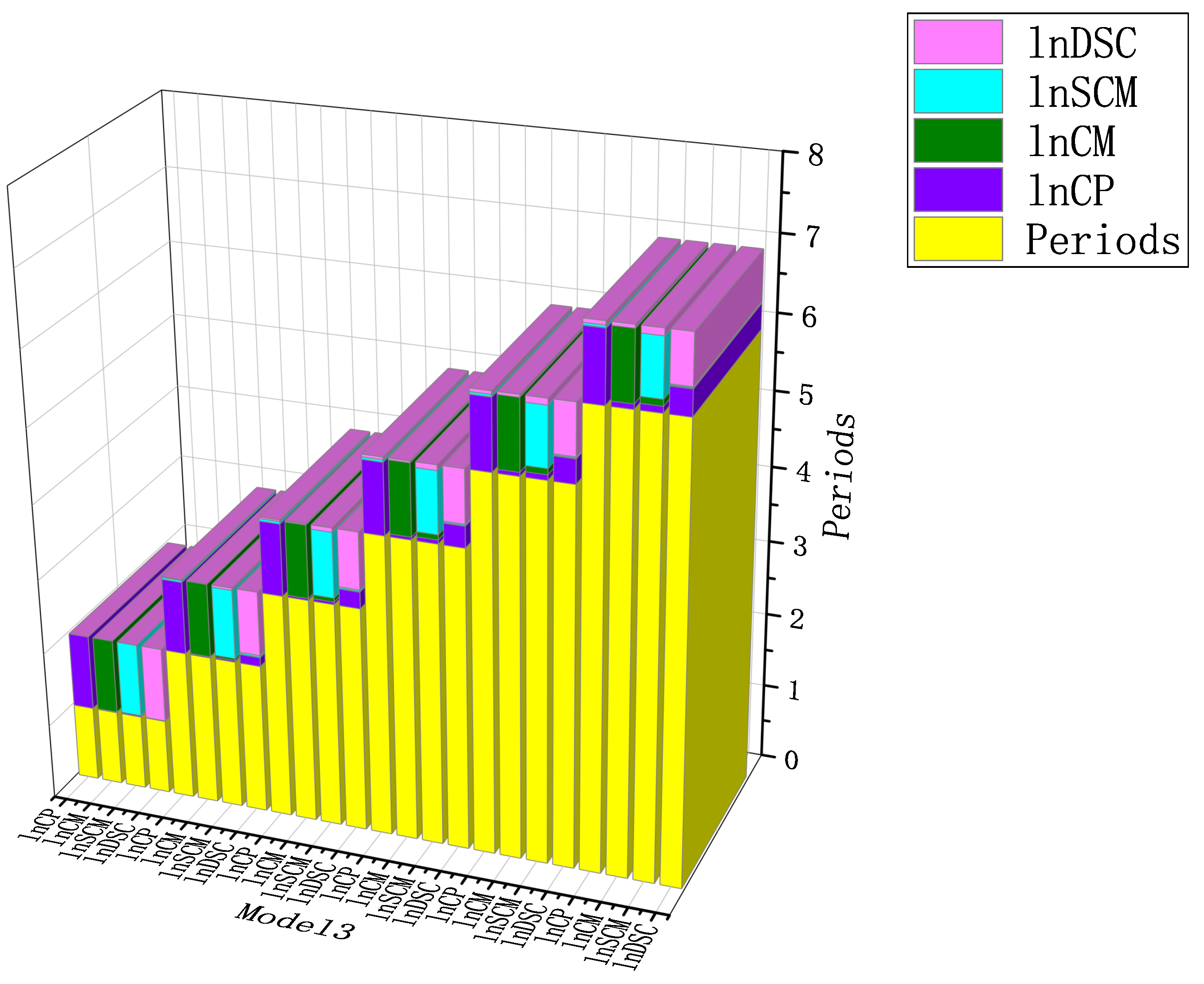
3.5. Variance Decomposition
3.6. Analysis of Regression Results
3.6.1. Regression Results
3.6.2. Testing
4. Conclusions and Recommendations
4.1. Conclusions
4.2. Recommendations
5. Discussion
5.1. Insufficient Research
5.2. Future Perspectives
Author Contributions
Funding
Data Availability Statement
Acknowledgments
Conflicts of Interest
Appendix A

| Variables | Periods | lnR&D | lnCM | lnSCM | lnDSC | |
|---|---|---|---|---|---|---|
| Model1 | lnR&D | 1.000 | 1.000 | 0.000 | 0.000 | 0.000 |
| lnCM | 1.000 | 0.000 | 1.000 | 0.000 | 0.000 | |
| lnSCM | 1.000 | 0.002 | 0.001 | 0.997 | 0.000 | |
| lnDSC | 1.000 | 0.007 | 0.002 | 0.001 | 0.991 | |
| lnR&D | 2.000 | 0.994 | 0.001 | 0.001 | 0.004 | |
| lnCM | 2.000 | 0.006 | 0.994 | 0.000 | 0.001 | |
| lnSCM | 2.000 | 0.004 | 0.014 | 0.962 | 0.020 | |
| lnDSC | 2.000 | 0.010 | 0.001 | 0.008 | 0.981 | |
| lnR&D | 3.000 | 0.985 | 0.002 | 0.002 | 0.010 | |
| lnCM | 3.000 | 0.015 | 0.983 | 0.000 | 0.001 | |
| lnSCM | 3.000 | 0.006 | 0.024 | 0.933 | 0.036 | |
| lnDSC | 3.000 | 0.013 | 0.001 | 0.011 | 0.974 | |
| lnR&D | 4.000 | 0.975 | 0.003 | 0.003 | 0.019 | |
| lnCM | 4.000 | 0.027 | 0.971 | 0.000 | 0.002 | |
| lnSCM | 4.000 | 0.009 | 0.030 | 0.915 | 0.046 | |
| lnDSC | 4.000 | 0.017 | 0.002 | 0.013 | 0.968 | |
| lnR&D | 5.000 | 0.965 | 0.003 | 0.004 | 0.028 | |
| lnCM | 5.000 | 0.040 | 0.958 | 0.000 | 0.002 | |
| lnSCM | 5.000 | 0.012 | 0.035 | 0.902 | 0.051 | |
| lnDSC | 5.000 | 0.021 | 0.003 | 0.013 | 0.963 | |
| lnR&D | 6.000 | 0.955 | 0.004 | 0.005 | 0.036 | |
| lnCM | 6.000 | 0.053 | 0.945 | 0.000 | 0.002 | |
| lnSCM | 6.000 | 0.015 | 0.037 | 0.894 | 0.054 | |
| lnDSC | 6.000 | 0.025 | 0.004 | 0.014 | 0.957 | |
| Variables | Periods | lnR&D | lnSCM | lnGrowth | lnDSC | |
| Model2 | lnR&D | 1.000 | 1.000 | 0.000 | 0.000 | 0.000 |
| lnSCM | 1.000 | 0.004 | 0.996 | 0.000 | 0.000 | |
| lnGrowth | 1.000 | 0.000 | 0.006 | 0.994 | 0.000 | |
| lnDSC | 1.000 | 0.012 | 0.012 | 0.001 | 0.975 | |
| lnR&D | 2.000 | 0.999 | 0.000 | 0.001 | 0.001 | |
| lnSCM | 2.000 | 0.013 | 0.902 | 0.014 | 0.071 | |
| lnGrowth | 2.000 | 0.000 | 0.006 | 0.992 | 0.002 | |
| lnDSC | 2.000 | 0.016 | 0.036 | 0.019 | 0.929 | |
| lnR&D | 3.000 | 0.997 | 0.000 | 0.001 | 0.002 | |
| lnSCM | 3.000 | 0.024 | 0.811 | 0.024 | 0.141 | |
| lnGrowth | 3.000 | 0.001 | 0.007 | 0.988 | 0.005 | |
| lnDSC | 3.000 | 0.021 | 0.049 | 0.033 | 0.897 | |
| lnR&D | 4.000 | 0.996 | 0.000 | 0.001 | 0.003 | |
| lnSCM | 4.000 | 0.034 | 0.748 | 0.031 | 0.188 | |
| lnGrowth | 4.000 | 0.001 | 0.007 | 0.984 | 0.007 | |
| lnDSC | 4.000 | 0.028 | 0.057 | 0.040 | 0.876 | |
| lnR&D | 5.000 | 0.995 | 0.000 | 0.001 | 0.004 | |
| lnSCM | 5.000 | 0.043 | 0.706 | 0.034 | 0.217 | |
| lnGrowth | 5.000 | 0.001 | 0.008 | 0.982 | 0.010 | |
| lnDSC | 5.000 | 0.034 | 0.061 | 0.045 | 0.860 | |
| lnR&D | 6.000 | 0.994 | 0.000 | 0.001 | 0.005 | |
| lnSCM | 6.000 | 0.052 | 0.677 | 0.037 | 0.235 | |
| lnGrowth | 6.000 | 0.001 | 0.008 | 0.980 | 0.011 | |
| lnDSC | 6.000 | 0.041 | 0.063 | 0.048 | 0.849 | |
| Model3 | lnCP | 1.000 | 1.000 | 0.000 | 0.000 | 0.000 |
| lnCM | 1.000 | 0.009 | 0.991 | 0.000 | 0.000 | |
| lnSCM | 1.000 | 0.017 | 0.003 | 0.979 | 0.000 | |
| lnDSC | 1.000 | 0.002 | 0.004 | 0.001 | 0.993 | |
| lnCP | 2.000 | 0.966 | 0.000 | 0.027 | 0.007 | |
| lnCM | 2.000 | 0.015 | 0.980 | 0.000 | 0.005 | |
| lnSCM | 2.000 | 0.020 | 0.029 | 0.920 | 0.031 | |
| lnDSC | 2.000 | 0.118 | 0.007 | 0.023 | 0.852 | |
| lnCP | 3.000 | 0.947 | 0.001 | 0.032 | 0.021 | |
| lnCM | 3.000 | 0.025 | 0.962 | 0.000 | 0.014 | |
| lnSCM | 3.000 | 0.034 | 0.051 | 0.859 | 0.056 | |
| lnDSC | 3.000 | 0.219 | 0.008 | 0.020 | 0.753 | |
| lnCP | 4.000 | 0.933 | 0.002 | 0.031 | 0.034 | |
| lnCM | 4.000 | 0.037 | 0.939 | 0.000 | 0.024 | |
| lnSCM | 4.000 | 0.052 | 0.066 | 0.809 | 0.072 | |
| lnDSC | 4.000 | 0.278 | 0.009 | 0.017 | 0.696 | |
| lnCP | 5.000 | 0.922 | 0.003 | 0.030 | 0.044 | |
| lnCM | 5.000 | 0.051 | 0.914 | 0.000 | 0.035 | |
| lnSCM | 5.000 | 0.069 | 0.076 | 0.771 | 0.083 | |
| lnDSC | 5.000 | 0.312 | 0.010 | 0.015 | 0.663 | |
| lnCP | 6.000 | 0.914 | 0.005 | 0.030 | 0.052 | |
| lnCM | 6.000 | 0.065 | 0.890 | 0.000 | 0.045 | |
| lnSCM | 6.000 | 0.083 | 0.083 | 0.742 | 0.092 | |
| lnDSC | 6.000 | 0.332 | 0.012 | 0.014 | 0.642 | |
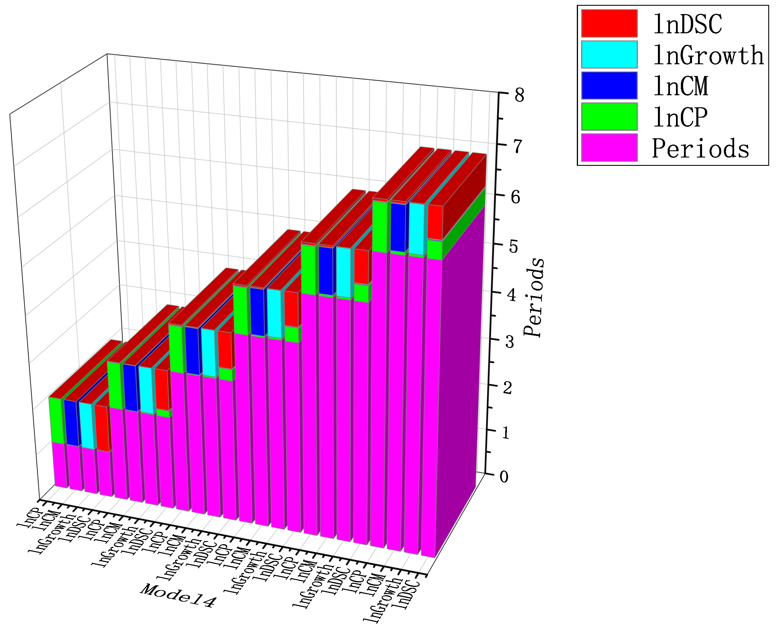
| Variables | Periods | lnCP | lnCM | lnGrowth | lnDSC | |
| Model4 | lnCP | 1.000 | 1.000 | 0.000 | 0.000 | 0.000 |
| lnCM | 1.000 | 0.008 | 0.992 | 0.000 | 0.000 | |
| lnGrowth | 1.000 | 0.002 | 0.001 | 0.997 | 0.000 | |
| lnDSC | 1.000 | 0.000 | 0.004 | 0.005 | 0.991 | |
| lnCP | 2.000 | 0.983 | 0.000 | 0.007 | 0.010 | |
| lnCM | 2.000 | 0.011 | 0.980 | 0.004 | 0.005 | |
| lnGrowth | 2.000 | 0.021 | 0.002 | 0.976 | 0.002 | |
| lnDSC | 2.000 | 0.139 | 0.006 | 0.006 | 0.850 | |
| lnCP | 3.000 | 0.966 | 0.001 | 0.010 | 0.023 | |
| lnCM | 3.000 | 0.019 | 0.960 | 0.008 | 0.013 | |
| lnGrowth | 3.000 | 0.033 | 0.002 | 0.961 | 0.004 | |
| lnDSC | 3.000 | 0.237 | 0.008 | 0.008 | 0.747 | |
| lnCP | 4.000 | 0.954 | 0.001 | 0.012 | 0.033 | |
| lnCM | 4.000 | 0.031 | 0.936 | 0.010 | 0.023 | |
| lnGrowth | 4.000 | 0.040 | 0.002 | 0.951 | 0.007 | |
| lnDSC | 4.000 | 0.294 | 0.010 | 0.011 | 0.685 | |
| lnCP | 5.000 | 0.944 | 0.002 | 0.013 | 0.041 | |
| lnCM | 5.000 | 0.045 | 0.910 | 0.012 | 0.033 | |
| lnGrowth | 5.000 | 0.045 | 0.002 | 0.944 | 0.009 | |
| lnDSC | 5.000 | 0.327 | 0.013 | 0.013 | 0.647 | |
| lnCP | 6.000 | 0.937 | 0.003 | 0.013 | 0.047 | |
| lnCM | 6.000 | 0.059 | 0.884 | 0.014 | 0.044 | |
| lnGrowth | 6.000 | 0.048 | 0.002 | 0.939 | 0.011 | |
| lnDSC | 6.000 | 0.348 | 0.015 | 0.015 | 0.622 | |
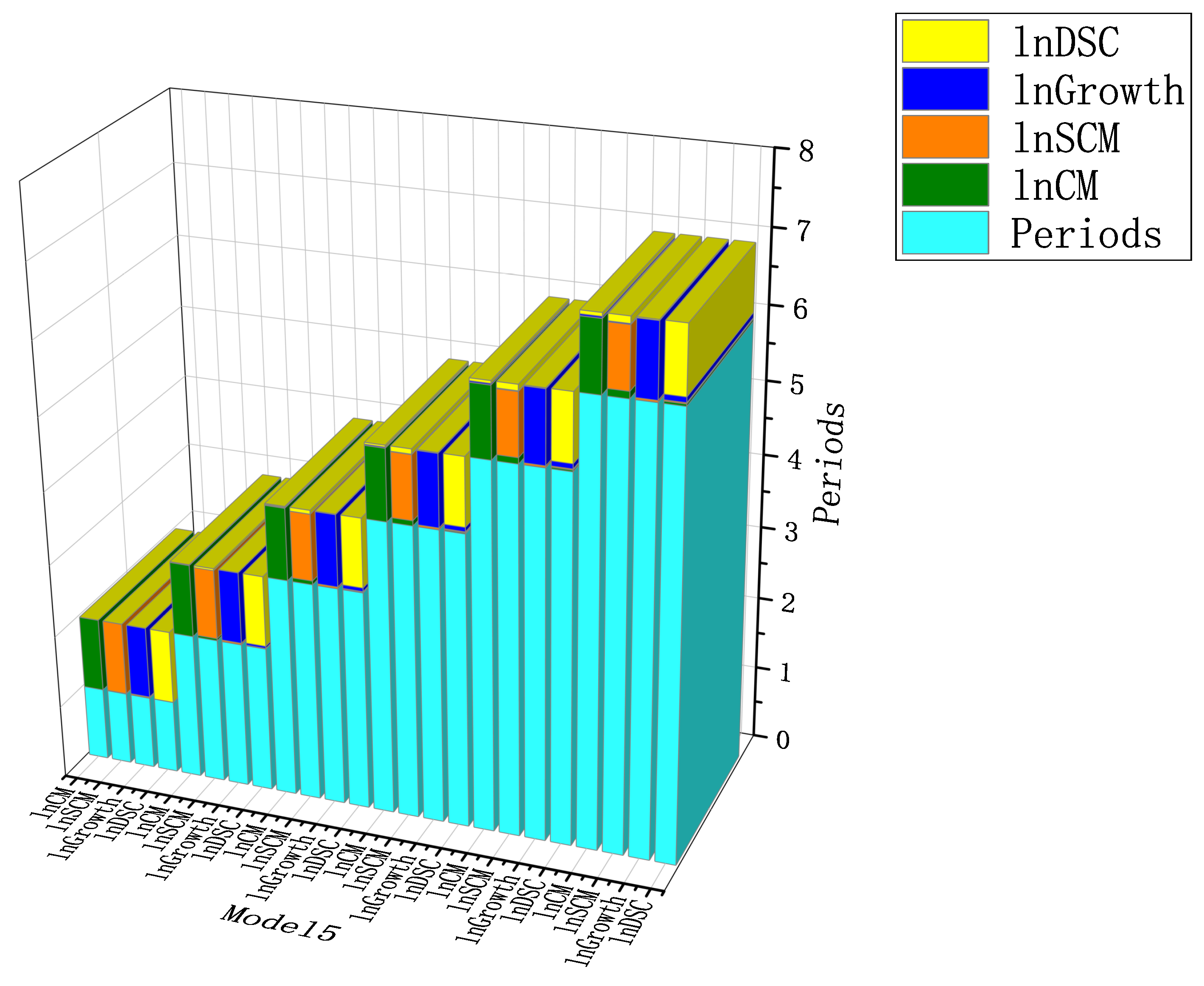
| Model5 | lnCM | 1.000 | 1.000 | 0.000 | 0.000 | 0.000 |
| lnSCM | 1.000 | 0.006 | 0.994 | 0.000 | 0.000 | |
| lnGrowth | 1.000 | 0.001 | 0.017 | 0.982 | 0.000 | |
| lnDSC | 1.000 | 0.000 | 0.000 | 0.002 | 0.998 | |
| lnCM | 2.000 | 0.990 | 0.001 | 0.005 | 0.004 | |
| lnSCM | 2.000 | 0.029 | 0.945 | 0.000 | 0.026 | |
| lnGrowth | 2.000 | 0.001 | 0.022 | 0.974 | 0.002 | |
| lnDSC | 2.000 | 0.002 | 0.007 | 0.029 | 0.962 | |
| lnCM | 3.000 | 0.976 | 0.001 | 0.010 | 0.013 | |
| lnSCM | 3.000 | 0.051 | 0.896 | 0.003 | 0.050 | |
| lnGrowth | 3.000 | 0.001 | 0.024 | 0.969 | 0.006 | |
| lnDSC | 3.000 | 0.007 | 0.011 | 0.048 | 0.934 | |
| lnCM | 4.000 | 0.960 | 0.002 | 0.014 | 0.024 | |
| lnSCM | 4.000 | 0.068 | 0.858 | 0.007 | 0.067 | |
| lnGrowth | 4.000 | 0.002 | 0.024 | 0.965 | 0.009 | |
| lnDSC | 4.000 | 0.014 | 0.014 | 0.058 | 0.914 | |
| lnCM | 5.000 | 0.944 | 0.003 | 0.018 | 0.035 | |
| lnSCM | 5.000 | 0.081 | 0.828 | 0.010 | 0.080 | |
| lnGrowth | 5.000 | 0.003 | 0.024 | 0.962 | 0.011 | |
| lnDSC | 5.000 | 0.021 | 0.015 | 0.065 | 0.899 | |
| lnCM | 6.000 | 0.928 | 0.004 | 0.022 | 0.046 | |
| lnSCM | 6.000 | 0.092 | 0.805 | 0.013 | 0.090 | |
| lnGrowth | 6.000 | 0.003 | 0.024 | 0.960 | 0.013 | |
| lnDSC | 6.000 | 0.029 | 0.016 | 0.069 | 0.886 |
References
- FAO; IFAD; UNICEF; WFP; WHO. The State of Food Security and Nutrition in the World 2022. Repurposing Food and Agricultural Policies to Make Healthy Diets More Affordable; FAO: Rome, Italy, 2022. [Google Scholar] [CrossRef]
- UN. World Bank: World Food Security Situation Remains a Concern. 2022. Available online: https://news.un.org/zh/story/2022/08/1107792 (accessed on 16 November 2022).
- Xi, J. Holding High the Great Banner of Socialism with Chinese Characteristics Uniting Struggles for the Comprehensive Construction of a Modern Socialist Country—Report at the 20th National Congress of the Communist Party of China. 2022. Available online: http://www.qstheory.cn/yaowen/2022-10/25/c_1129079926.htm (accessed on 16 November 2022).
- Mertens, J.; Germer, J.; Siqueira, J.A.; Sauerborn, J. Spondias tuberosa Arruda (Anacardiaceae), a threatened tree of the Brazilian Caatinga? Braz. J. Biol. 2016, 77, 542–552. [Google Scholar] [CrossRef] [PubMed]
- Susanti, A.; Marhaento, H.; Permadi, D.B.; Imron, M.A.; Maimunah, S.; Susanto, D.; Lembasi, M. Smallholder farmers’ perception on oil palm agroforestry. IOP Conf. Ser. Earth Environ. Sci. 2020, 449, 012056. [Google Scholar] [CrossRef]
- Röhrig, N.; Hassler, M.; Roesler, T. Silvopastoral production as part of alternative food networks: Agroforestry systems in Umbria and Lazio, Italy. Agroecol. Sustain. Food Syst. 2021, 45, 654–672. [Google Scholar] [CrossRef]
- Branca, G.; Arslan, A.; Paolantonio, A.; Grewer, U.; Cattaneo, A.; Cavatassi, R.; Vetter, S. Assessing the economic and mitigation benefits of climate-smart agriculture and its implications for political economy: A case study in Southern Africa. J. Clean. Prod. 2021, 285, 125161. [Google Scholar] [CrossRef]
- Liu, H.; Fan, L.; Shao, Z. Threshold effects of energy consumption, technological innovation, and supply chain management on enterprise performance in China’s manufacturing industry. J. Environ. Manag. 2021, 300, 113687. [Google Scholar] [CrossRef] [PubMed]
- Liu, H.; Liu, J.; Li, Q. Asymmetric effects of economic development, agroforestry development, energy consumption, and population size on CO2 emissions in China. Sustainability 2022, 14, 7144. [Google Scholar] [CrossRef]
- Fan, L.; Liu, H.; Shao, Z.; Li, C. Panel data analysis of energy conservation and emission reduction on high-quality development of logistics industry in Yangtze River Delta of China. Environ. Sci. Pollut. Res. 2022, 29, 78361–78380. [Google Scholar] [CrossRef]
- Bayala, J.; Prieto, I. Water acquisition, sharing and redistribution by roots: Applications to agroforestry systems. Plant Soil. 2020, 453, 17–28. [Google Scholar] [CrossRef]
- Correa, C.; Alves, Y.A.; Souza, C.G.; Boloy, R.A.M. Brazil and the world market in the development of technologies for the production of second-generation ethanol. Alex. Eng. J. 2022, 9. [Google Scholar] [CrossRef]
- Matos, S.; Viardot, E.; Sovacool, B.K.; Geels, F.W.; Xiong, Y. Innovation and climate change: A review and introduction to the special issue. Technovation 2022, 117, 102612. [Google Scholar] [CrossRef]
- Sovacool, B.K. Who are the victims of low-carbon transitions? Towards a political ecology of climate change mitigation. Energy Soc. Sci. 2021, 73, 101916. [Google Scholar] [CrossRef]
- UNGC-Accenture. A Call to Climate Action. 2015. Available online: https://www.unglobalcompact.org/library/3551 (accessed on 16 November 2022).
- Henttonen, K.; Lehtimäki, H. Open innovation in SMEs: Collaboration modes and strategies for commercialization in technology-intensive companies in forestry industry. Eur. J. Innov. Manag. 2017, 20, 329–347. [Google Scholar] [CrossRef]
- Pynnönen, S.; Haltia, E.; Hujala, T. Digital forest information platform as service innovation: Finnish Metsaan. fi service use, users and utilisation. For. Police Econ. 2021, 125, 102404. [Google Scholar] [CrossRef]
- Olopainen, J.; Mattila, O.; Pöyry, E.; Parvinen, P. Applying design science research methodology in the development of virtual reality forest management services. For. Police Econ. 2020, 116, 102190. [Google Scholar] [CrossRef]
- Purkus, A.; Lüdtke, J. A systemic evaluation framework for a multi-actor, forest-based bioeconomy governance process: The German Charter for Wood 2.0 as a case study. For. Police Econ. 2020, 113, 102113. [Google Scholar] [CrossRef]
- Pelai, R.; Hagerman, S.M.; Kozak, R. Biotechnologies in agriculture and forestry: Governance insights from a comparative systematic review of barriers and recommendations. For. Police Econ. 2020, 117, 102191. [Google Scholar] [CrossRef]
- Lawrence, A.; Wong, J.L.G.; Molteno, S. Fostering social enterprise in woodlands: Challenges for partnerships supporting social innovation. For. Police Econ. 2020, 118, 102221. [Google Scholar] [CrossRef]
- Ludvig, A.; Sarkki, S.; Weiss, G.; Živojinović, I. Policy impacts on social innovation in forestry and back: Institutional change as a driver and outcome. For. Police Econ. 2021, 122, 102335. [Google Scholar] [CrossRef]
- Wilkes-Allemann, J.; Ludvig, A.; Hogl, K. Innovation development in forest ecosystem services: A comparative mountain bike trail study from Austria and Switzerland. For. Police Econ. 2020, 115, 102158. [Google Scholar] [CrossRef]
- Boyer, J.; Touzard, J.M. To what extent do an innovation system and cleaner technological regime affect the decision-making process of climate change adaptation? Evidence from wine producers in three wine clusters in France. J. Clean. Prod. 2021, 315, 128218. [Google Scholar] [CrossRef]
- Zhao, J.; Pongtornkulpanich, A.; Cheng, W. The Impact of Board Size on Green Innovation in China’s Heavily Polluting Enterprises: The Mediating Role of Innovation Openness. Sustainability 2022, 14, 8632. [Google Scholar] [CrossRef]
- Weiss, G.; Hansen, E.; Ludvig, A.; Nybakk, E.; Toppinen, A. Innovation governance in the forest sector: Reviewing concepts, trends and gaps. For. Policy Econ. 2021, 130, 102506. [Google Scholar] [CrossRef]
- Innes, J.L. The promotion of ‘innovation’ in forestry: A role for government or others? J. Integr. Environ. Sci. 2009, 6, 201–215. [Google Scholar] [CrossRef]
- Kim, S.; Park, K.C. Government funded R&D collaboration and it’s impact on SME’s business performance. J. Inf. 2021, 15, 101197. [Google Scholar] [CrossRef]
- Schuhmacher, A.; Wilisch, L.; Kuss, M.; Kandelbauer, A.; Hinder, M.; Gassmann, O. R&D efficiency of leading pharmaceutical companies–A 20-year analysis. Drug Discov. Today 2021, 26, 1784–1789. [Google Scholar] [CrossRef]
- Boeing, P.; Eberle, J.; Howell, A. The impact of China’s R&D subsidies on R&D investment, technological upgrading and economic growth. Technol. Forecast. Soc. 2022, 174, 121212. [Google Scholar] [CrossRef]
- Da Silveira Pontes, L.; Giostri, A.F.; Baldissera, T.C.; Barro, R.S.; Stafin, G.; Porfírio-da-Silva, V.; César de Faccio Carvalho, P. Interactive effects of trees and nitrogen supply on the agronomic characteristics of warm-climate grasses. Agron. J. 2016, 108, 1531–1541. [Google Scholar] [CrossRef]
- Wu, Z.; Fan, X.; Zhu, B.; Xia, J.; Zhang, L.; Wang, P. Do government subsidies improve innovation investment for new energy firms: A quasi-natural experiment of China’s listed companies. Technol. Forecast. Soc. 2022, 175, 121418. [Google Scholar] [CrossRef]
- Harymawan, I.; Agustia, D.; Nasih, M.; Inayati, A.; Nowland, J. Remuneration committees, executive remuneration, and firm performance in Indonesia. Heliyon 2020, 6, e03452. [Google Scholar] [CrossRef]
- Wang, H.; Wang, W.; Alhaleh, S.E.A. Mixed ownership and financial investment: Evidence from Chinese state-owned enterprises. Econ. Anal. Policy 2021, 70, 159–171. [Google Scholar] [CrossRef]
- FAO. Responsible Business Conduct (RBC) in Agriculture. 2022. Available online: https://www.fao.org/res-ponsible-business-conduct-in-agriculture/en/ (accessed on 6 September 2022).
- Siregar, M.Y.; Mardiana, M. Effect of Quick Ratio, Total Asset Turnover, and Receivable Turnover on Return on Assets in Food and Beverages Companies Listed on the Indonesia Stock Exchange (IDX). BIRCI-J. 2022, 5, 5347–5359. [Google Scholar] [CrossRef]
- Zimon, G.; Babenko, V.; Sadowska, B.; Chudy-Laskowska, K.; Gosik, B. Inventory Management in SMEs Operating in Polish Group Purchasing Organizations during the COVID-19 Pandemic. Risks 2021, 9, 63. [Google Scholar] [CrossRef]
- Mauris, F.I.; Nora, A.R. The effect of collaterallizable assets, growth in net assets, liquidity, leverage and profitability on dividend policy. BIRCI-J. 2019, 4, 937–950. [Google Scholar] [CrossRef]
- Kang, M.Y. Sustainable Profit versus Unsustainable Growth: Are Venture Capital Investments and Governmental Support Medicines or Poisons? Sustainability 2020, 12, 7773. [Google Scholar] [CrossRef]
- Feng, Z.; Wu, Z. Local economy, asset location and REIT firm growth. J. Real Estate Financ. Econ. 2022, 65, 75–102. [Google Scholar] [CrossRef]
- Li, F.; Di, H. Analysis of the financing structure of China’s listed new energy companies under the goal of peak CO2 emissions and carbon neutrality. Energies 2021, 14, 5636. [Google Scholar] [CrossRef]
- Zhao, L.; Yang, S.; Wang, S.; Shen, J. Research on PPP Enterprise Credit Dynamic Prediction Model. Appl. Sci. 2022, 12, 10362. [Google Scholar] [CrossRef]
- Shi, W. Analyzing enterprise asset structure and profitability using cloud computing and strategic management accounting. PLoS ONE 2021, 16, e0257826. [Google Scholar] [CrossRef]
- Zhu, L.; Li, M.; Metawa, N. Financial risk evaluation Z-score model for intelligent IoT-based enterprises. Inf. Process. Manag. 2021, 58, 102692. [Google Scholar] [CrossRef]
- Santos, E.; Lisboa, I.; Eugénio, T. The Financial Performance of Family versus Non-Family Firms Operating in Nautical Tourism. Sustainability 2022, 14, 1693. [Google Scholar] [CrossRef]
- Wang, M.; Zhao, X.; Gong, Q.; Ji, Z. Measurement of regional green economy sustainable development ability based on entropy weight-topsis-coupling coordination degree—A case study in shandong province, China. Sustainability 2019, 11, 280. [Google Scholar] [CrossRef]
- Jin, H.; Qian, X.; Chin, T.; Zhang, H. A global assessment of sustainable development based on modification of the human development index via the entropy method. Sustainability 2020, 12, 3251. [Google Scholar] [CrossRef]


| Variable | Obs | Mean | Std. dev. | Min | Max |
|---|---|---|---|---|---|
| code | 480 | 20.5 | 11.555440 | 1 | 40 |
| year | 480 | 2015.5 | 3.455654 | 2010 | 2021 |
| R&D Innovation (R&D) | 480 | 0.012909 | 0.021338 | 0.000275 | 0.167384 |
| Corporate Management (CM) | 480 | 0.022126 | 0.020605 | 0.002041 | 0.147030 |
| Supply Chain Management (SCM) | 480 | 0.005963 | 0.020917 | 0.000229 | 0.150879 |
| Growth Capability (Growth) | 480 | 0.001059 | 0.005621 | 0.000167 | 0.121723 |
| Debt Servicing Capacity (DSC) | 480 | 0.001957 | 0.001050 | 0.000908 | 0.013591 |
| Corporate Performance (CP) | 480 | 0.000416 | 0.000055 | 0.000183 | 0.001052 |
| Variables | Indicators | Weights |
|---|---|---|
| Research and Development Innovation (R&D) | X1 = Number of R&D staff | 0.025348 |
| X2 = Number of R&D staff as a percentage (%) | 0.015784 | |
| X3 = Amount of R&D investment | 0.033095 | |
| X4 = R&D investment as a percentage of operating revenue (%) | 0.023971 | |
| X5 = Amount of R&D inputs (expenses) expensed | 0.033869 | |
| X6 = Amount of R&D investment (expenditure) capitalized | 0.076709 | |
| X7 = Capitalized R&D investment (expenditure) as a percentage of R&D investment (%) | 0.051822 | |
| Corporate Management (CM) | X8 = Equity concentration indicator1 (%) | 0.003983 |
| X9 = Board size | 0.00534 | |
| X10 = Whether the actual controller is the chairman or general manager | 0.018003 | |
| X11 = number of shares held by the chairman | 0.046478 | |
| X12 = Chairman’s shareholding (%) | 0.081623 | |
| X13 = Total compensation of top three executives | 0.037186 | |
| X14 = Total executive compensation | 0.074338 | |
| X15 = Number of executives | 0.001475 | |
| X16 = number of shares held by executives | 0.050831 | |
| Supply Chain Management (SCM) | X17 = Net Inventory | 0.021952 |
| X18 = Accounts payable turnover ratio | 0.095599 | |
| X19 = Total asset turnover ratio | 0.033429 | |
| X20 = Accounts receivable turnover ratio | 0.062244 | |
| X21 = Inventory turnover ratio | 0.051612 | |
| Growth capacity (Growth) | X22 = Revenue on net assets growth rate | 0.012597 |
| X23 = Net profit growth rate | 0.000108 | |
| X24 = Operating income growth rate | 0.121145 | |
| X25 = Net asset per share growth rate | 0.000072 | |
| Debt Service Capacity (DSC) | X26 = Cash ratio | 0.013378 |
| X27 = Equity ratio | 0.003005 | |
| X28 = Gearing ratio | 0.003859 | |
| Corporate performance (CP) | X29 = Revenue on net assets | 0.000133 |
| X30 = Revenue on investment | 0.000860 | |
| X31 = operating profit margin | 0.000059 | |
| X32 = Revenue on total assets | 0.000090 |
| Variable | IPS | LLC | ADF–Fisher | PP–Fisher |
|---|---|---|---|---|
| lnR&D | −10.332 *** | −23.820 *** | 541.025 *** | 979.315 *** |
| (0.000) | (0.000) | (0.000) | (0.000) | |
| lnCM | −8.779 *** | −23.812 *** | 566.063 *** | 1097.357 *** |
| (0.000) | (0.000) | (0.000) | (0.000) | |
| lnSCM | −11.199 *** | −25.701 *** | 485.274 *** | 1119.771 *** |
| (0.000) | (0.000) | (0.000) | (0.000) | |
| lnGrowth | −10.172 *** | −270.127 *** | 498.233 *** | 1634.031 *** |
| (0.000) | (0.000) | (0.000) | (0.000) | |
| lnDSC | −10.122 *** | −25.230 *** | 426.216 *** | 1224.023 *** |
| (0.000) | (0.000) | (0.000) | (0.000) | |
| lnCP | −5.965 *** | −26.781 *** | 331.648 *** | 1398.684 *** |
| (0.000) | (0.000) | (0.000) | (0.000) |
| Model | Cause and Effect | chi2 | df | p-Value |
|---|---|---|---|---|
| Model 1 | lnR&D → lnSCM | 0.084 | 1 | 0.772 |
| lnCM → lnSCM | 3.709 ** | 1 | 0.054 | |
| lnDSC→ lnSCM | 3.546 ** | 1 | 0.060 | |
| ALL → lnSCM | 10.913 *** | 3 | 0.012 | |
| Model 2 | lnGrowth→lnSCM | 7.316 ** | 2 | 0.026 |
| ALL → lnSCM | 17.730 *** | 6 | 0.007 | |
| lnR&D → lnDSC | 4.633 * | 2 | 0.099 | |
| ALL → lnDSC | 14.198 ** | 6 | 0.027 | |
| Model 3 | lnCM → lnSCM | 3.853 ** | 1 | 0.050 |
| lnDSC→ lnSCM | 5.1415 ** | 1 | 0.023 | |
| ALL → lnSCM | 12.266 *** | 3 | 0.007 | |
| lnCP → lnDSC | 3.845 ** | 1 | 0.050 | |
| Model 4 | lnDSC→ lnCP | 4.836 * | 2 | 0.089 |
| lnCM → lnDSC | 0.948 | 2 | 0.622 | |
| lnGrowth→lnDSC | 5.123 * | 2 | 0.077 | |
| ALL → lnDSC | 16.573 *** | 6 | 0.011 | |
| Model 5 | lnCM → lnSCM | 9.649 *** | 2 | 0.008 |
| lnGrowth→lnSCM | 10.207 *** | 2 | 0.006 | |
| lnDSC→ lnSCM | 8.666 *** | 2 | 0.013 | |
| ALL → lnSCM | 28.840 *** | 6 | 0.000 |
| Variables | lnCP | |||
|---|---|---|---|---|
| OLS | 2SLS | LIML | GMM | |
| lnR&D | 0.000371 | 0.0249 *** | 0.0269 *** | 0.0203 *** |
| (0.0014) | (0.0067) | (0.0074) | (0.0050) | |
| lnCM | 0.00418 * | −0.0120 ** | −0.0133 ** | −0.00861 * |
| (0.0024) | (0.0060) | (0.0064) | (0.0049) | |
| lnDSC | −0.0278 *** | −0.0210 * | −0.0204 * | −0.0251 ** |
| (0.0093) | (0.0112) | (0.0114) | (0.0101) | |
| Constant | −7.948 *** | −7.841 *** | −7.832 *** | −7.876 *** |
| (0.0586) | (0.0763) | (0.0790) | (0.0666) | |
| Observations | 480 | 480 | 480 | 480 |
| Intermediate Variables | Effects | Observed Coefficient | Bootstrap Std. Err. |
|---|---|---|---|
| lnSCM | Indirect effect | 0.001266 *** | 0.000434 |
| Direct effect | −0.000895 | 0.001495 | |
| lnGrowth | Indirect effect | 0.000905 *** | 0.000198 |
| Direct effect | −0.000534 | 0.001467 | |
| Intermediate variables | z | p > z | Normal-based [95% conf.interval] |
| lnSCM | 2.91 | 0.004 | [0.000414, 0.002117] |
| −0.6 | 0.549 | [−0.003825, 0.002034] | |
| lnGrowth | 4.56 | 0.000 | [0.000516, 0.001294] |
| −0.36 | 0.716 | [−0.003410, 0.002342] |
Publisher’s Note: MDPI stays neutral with regard to jurisdictional claims in published maps and institutional affiliations. |
© 2022 by the authors. Licensee MDPI, Basel, Switzerland. This article is an open access article distributed under the terms and conditions of the Creative Commons Attribution (CC BY) license (https://creativecommons.org/licenses/by/4.0/).
Share and Cite
Liu, H.; Sun, M.; Gao, Q.; Liu, J.; Sun, Y.; Li, Q. What Affects the Corporate Performance of Listed Companies in China’s Agriculture and Forestry Industry? Agronomy 2022, 12, 3041. https://doi.org/10.3390/agronomy12123041
Liu H, Sun M, Gao Q, Liu J, Sun Y, Li Q. What Affects the Corporate Performance of Listed Companies in China’s Agriculture and Forestry Industry? Agronomy. 2022; 12(12):3041. https://doi.org/10.3390/agronomy12123041
Chicago/Turabian StyleLiu, Hui, Mingyu Sun, Qiang Gao, Jiwei Liu, Yong Sun, and Qun Li. 2022. "What Affects the Corporate Performance of Listed Companies in China’s Agriculture and Forestry Industry?" Agronomy 12, no. 12: 3041. https://doi.org/10.3390/agronomy12123041
APA StyleLiu, H., Sun, M., Gao, Q., Liu, J., Sun, Y., & Li, Q. (2022). What Affects the Corporate Performance of Listed Companies in China’s Agriculture and Forestry Industry? Agronomy, 12(12), 3041. https://doi.org/10.3390/agronomy12123041