Article

Single Plant Fertilization Using a Robotic Platform in an Organic Cropping Environment

by
Constantino Valero
1,*,
Anne Krus
1,
Christyan Cruz Ulloa
2,
Antonio Barrientos
2,
Juan José Ramírez-Montoro
1,
Jaime del Cerro
2 and
Pablo Guillén
1
1
LPF_Tagralia, Departamento de Ingeniería Agroforestal, ETSI Agronómica, Alimentaria y de Biosistemas, Universidad Politécnica de Madrid, Av. Puerta Hierro 2, 28040 Madrid, Spain
2
Centre for Automation and Robotics (CSIC-UPM), Consejo Superior de Investigaciones Científicas—Universidad Politécnica de Madrid, José Gutiérrez Abascal 2, 28006 Madrid, Spain
*
Author to whom correspondence should be addressed.
Agronomy 2022, 12(6), 1339; https://doi.org/10.3390/agronomy12061339
Submission received: 15 March 2022 / Revised: 13 May 2022 / Accepted: 28 May 2022 / Published: 31 May 2022
(This article belongs to the Special Issue Papers from AgEng2021)

Abstract

:
The growing demand for organically produced vegetables requires the adoption of new cropping systems such as strip-cropping. To counteract the additional labour mixed cropping entails, automation and robotics play a key role. This research focuses on the development of a proof-of-concept platform that combines optical sensors and an actuation system for targeted precision fertilization that encircles selected plants rather than a local field area. Two sensor types are used for the detection of a fertilisation need: a multispectral camera and light detection and ranging (LiDAR) devices in order to acquire information on plant health status and three-dimensional characterisation. Specific algorithms were developed to more accurately detect a change in fertilization need. An analysis of their results yields a prescription map for automatic fertilisation through a robotic arm. The relative location of the platform within the prescription map is essential for the correct application of fertilizers, and is acquired through live comparison of a LiDAR pushbroom with the known 3D world model. The geometry of each single plant is taken into account for the application of the sprayed fertiliser. This resulted in a reliable method for the detection of delayed growth and prototype localization within a changing natural environment without relying on external markers.

1. Introduction

The increase in food consumption around the world must be addressed by producers and technicians [1,2]. However, due to conventional agricultural practices, the environmental effect associated with the use of fertilisers and herbicides has increased [3]. Fortunately, precision agriculture allows producing higher quality products, through sustainable development [4], the use of technological tools, sensory systems [5,6], and modern actuation systems [7,8,9,10]. The Sureveg project [11] focuses on the application of diversified strip-cropping systems to intensive organic vegetable cultivation, the reuse of biodegradable waste, as well as the development of automated machinery for the management of strip-cropping systems.
The development of agricultural robotics accumulates several decades of history; however, only in recent years commercial prototypes have reached the market, and the real adoption of these technologies by farmers is very small [12,13,14]. Robotic platforms derived from research projects have been designed primarily to scout and sense crops [15,16] or the soil, and perform automated weeding on arable crops [17,18], while work has also been done also on robotic seeding [19], pesticide spraying [20], and harvesting [21], to mention some examples. Nevertheless, as far as we know, robotic fertilisation has not been properly studied, especially with respect to the application of organic fertilisers. Furthermore, the application of robotics to organic production requires a new approach, far from traditional monocultural farming systems, to include properly the agroecological context [22].
The objectives of this work were: designing and building a platform able to locate and characterize single plants along a crop row; extraction of plant features (health status, three-dimensional characterization) related to plant development in order to decide whether each single plant should be fertilised or not; and application of liquid fertiliser around targeted plants.
For this purpose, a proof-of-concept was proposed in the form of a manually displaced robotic prototype, containing three LiDAR sensors, a multispectral camera, and a 5 degree-of-freedom (DOF) manipulator. A nozzle connected to a tank of liquid organic fertilizer is used as the end-effector of the actuator.

2. Materials and Methods

The mobile platform implemented in the proof of concept of this work consists of different subsystems: the mobile structure with wheels, the robotic arm, the sensory system, the actuation system for the application of fertiliser, and the storage tank, as seen in Figure 1.

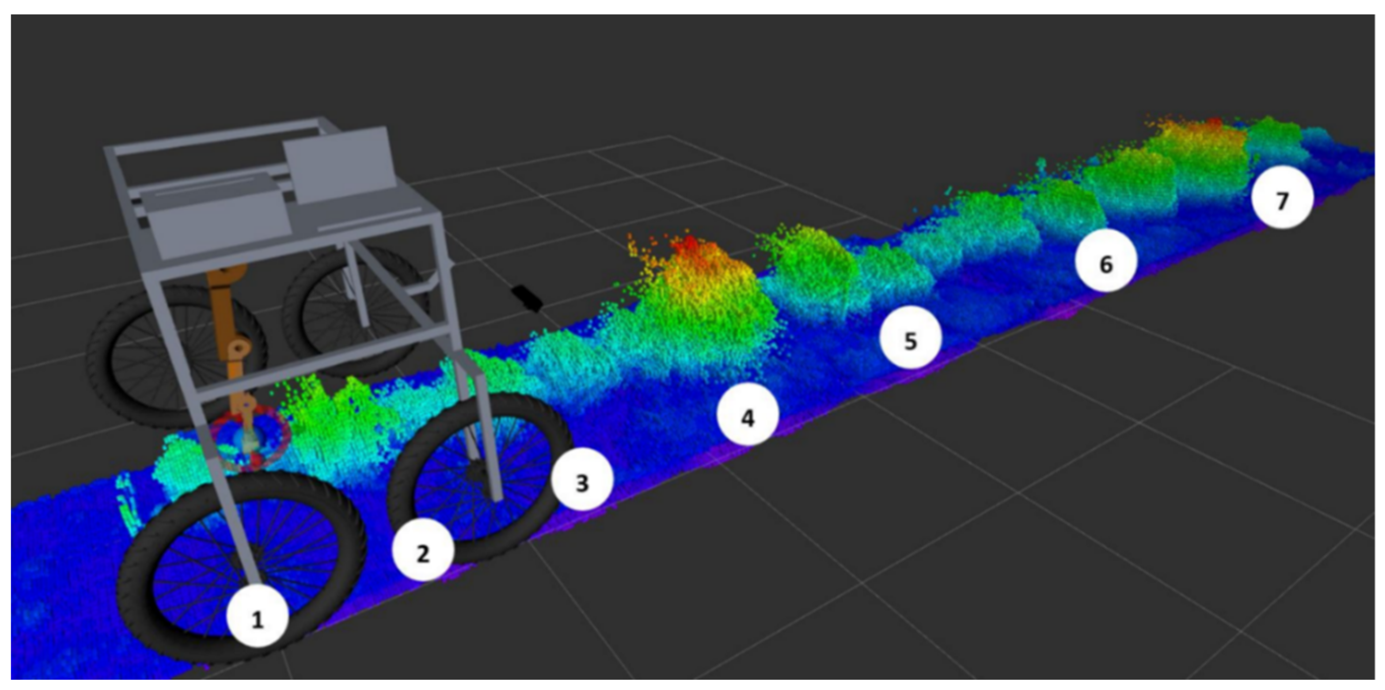
2.1. Mobile Structure
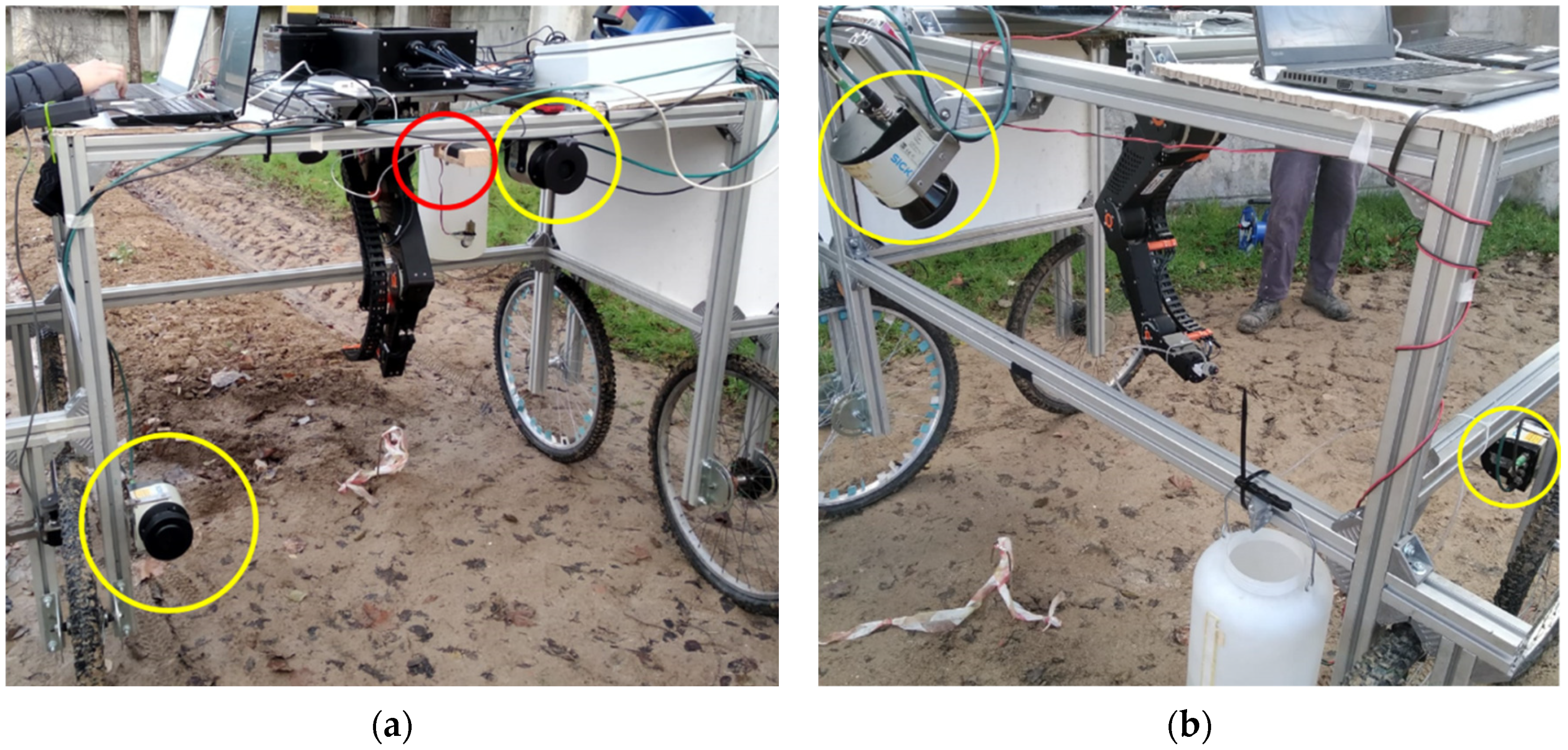
The mobile structure that supports the robot and sensory systems—actuation, was built with aluminium bars (Bosch Rexroth 45 × 45) and four wheels, according to previously established requirements in the framework of an organic stripped crop. The frame supports the different elements and does not rely on an autonomous traction system. Figure 1 shows the structure implemented with the sensory system indicated with coloured circles. At his stage of the work, displacement of the rig was performed manually, as automatic displacement is solved in many other prototypes, and the authors wanted to focus this research on sensing and actuation.

2.2. Sensory System

The sensory system relies mainly on two types of sensors: a multispectral camera and 3 LiDAR (light detection and ranging) devices. They were selected to provide combined information on vegetation health status (camera) and three-dimensional (3D) information on plant development (LiDAR). The multispectral camera (model Sequoia; Parrot Drones SAS, France) is used to obtain multispectral images and compute vegetation indices of plants. This camera was installed in the centre of the cart frame, to take pictures of the target plants from the zenith perspective. The Parrot Sequoia camera produces each image five times: 1.2 Mpixel images of green, red, red-edge, near-infrared channels, as well as a combined high-resolution (16 Mpixel, 10 bit) red, green, and blue (RGB) image. Each of the spectral images is obtained through a different lens. As a result, the images themselves show a slight translation with respect to one another. This effect is negligible when this type of camera is used onboard a drone, but in this case pictures were registered within a 1 m range to the plants. Image translation was assessed and corrected for automatically using the function ‘imgregtform’ in Matlab during image preprocessing.
The time lapse setting during image acquisition (3 s) in combination with a forward speed (0.55 m/s) generates a series of partially overlapping images that were stitched together using the software ‘Hugin Panorama’, as it is open source and allows for manual manipulation of automatically extracted features so that the exact same mosaicking operations can subsequently be applied to the other spectral bands. With the corrected mosaicked images, a series of vegetation indices were calculated for the entire field. The most optimal vegetation index can depend on the crop type and cultivar and can be optimised regarding the specific characteristics of the crops and soil spectra present in a certain field. In this work, results using the well-known normalized difference vegetation index (NDVI) are presented.
Furthermore, 3D data was gathered using 3 LiDAR devices (model LMS-111; SICK AG, Waldkirch, Germany) with the aim to create models of soil and plants from multiple perspectives. Each LiDAR uses an infrared rotating laser pulse, where the time of flight between emission and reflection in each rotational increment is used to calculate the distance of the sensor to any object. The reflectance intensity of the beam was found to not provide additional information in this setting and was ignored. From the cylindrical coordinates, each distance was converted to a Cartesian coordinate system, where the inclination of the sensor and the odometry data of the cart wheels were combined to provide the dimension perpendicular to the plane of rotation of the laser. This results in a 3D point cloud per LiDAR, describing the same crop row. These point clouds provide complementary information inherent to their varying angles and installation heights, where the majority of the surfaces are picked up by all LiDAR devices. This overlap was used to merge the point clouds into a high-resolution single point cloud, describing all surfaces within a crop row, in other words, both plant matter and non-plant matter such as soil. Besides information on crop architecture, the combined 3D world model facilitates motion planning of the robotic arm and the application of treatments in the adequate locations. Figure 1 shows the three sensor locations on the mobile structure: frontal 45-degree pushbroom, vertical (zenith view), and horizontal (across the row).

2.3. Sensing Algorithms

The sensing algorithms can be divided into two subcategories: multispectral sensing using the multi-spectral camera (aimed at searching for differences in plant health) and 3D sensing using the LiDAR (focused on detecting growth volume differences). Also, 3D information of crop rows will be used for the localization of the robot and the planification of the arm movement. Building the proper algorithms to locate and characterise single plants was an iterative process parallel to the data acquisition procedure; this is why more details about the sensing models built are included in the Results section, in order to be commented along with the findings.

2.4. Robotic Arm

The robotic arm acquired for the prototype (Robolink Igus CPR RL-DC-5 STEP RL-D-RBT-5532S-BF) has the following characteristics: a load capacity of 1.5 kg, 5 degrees of freedom, IP54 protection, and is able to follow point-to-point trajectories. The robot has a reach of 790 mm with a precision of 1 mm. This actuator weighs around 20 kg, including the electromechanical components and excluding the control and power elements.

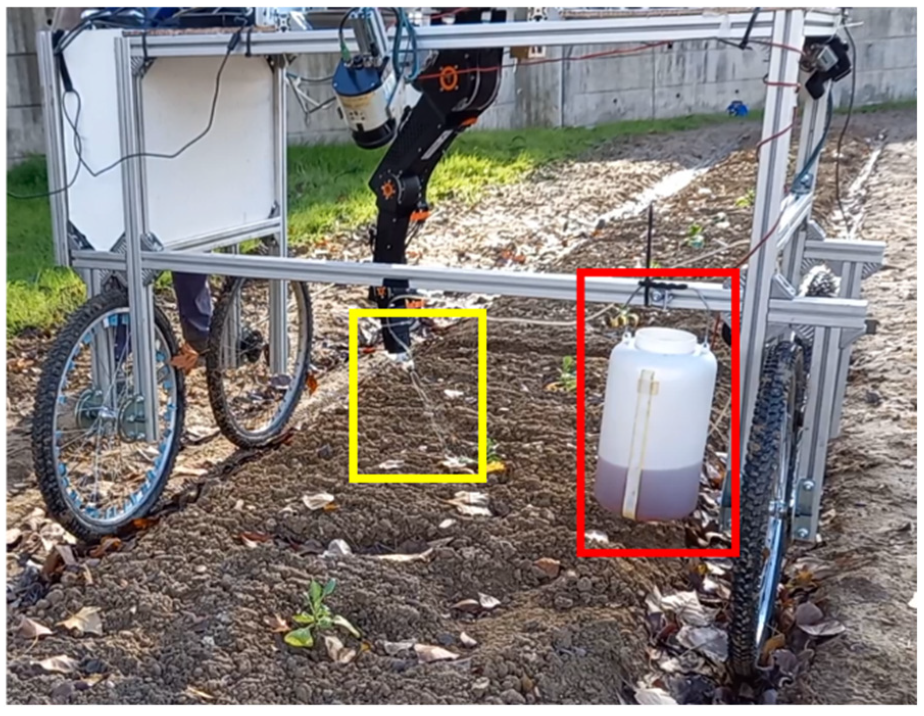
2.5. Fertilization System

The implemented actuation system consists of a tank containing a liquid treatment (Figure 2, highlighted in red), a hose from the tank to the robot tooltip, and a nozzle at the end to spray the liquid (Figure 2, indicated in yellow). In this way, the robotic arm can apply the liquid treatment in the desired position and orientation (on the soil around each plant), as shown in Figure 2. The actuation of the nozzle is carried out by means of a electronically controlled hydraulic motor.

2.6. Experimental Field and Crop

The field was located in ETSIAAB—UPM (40°26′33.1″ N, 3°43′41.9″ W) and consisted of a 50 m × 15 m test plot, on sandy-loamy soil, where organically fertilised crop strips were established and monitored during the growing season. The soil profile is very irregular since it has its origin in materials from construction waste. However, the phreatic level is high due to the proximity of the Manzanares river; in addition, crops were irrigated when needed using drip irrigation.
Regarding the fertiliser, a pre-crop application of 1 ton/ha of mature compost made from pig slurry and litter straw was applied and mixed with the soil, only to half of the field. In this way, the eastern part of each crop row (25 m) received more fertiliser than the western half, in order to create nutrient differences in the field before transplantation, which could generate later variances in early crop development, to be detected by the sensorized platform.
Subsequent robotic applications were carried out using a commercial water-soluble liquid fertilizer (3% nitrogen, 5% of potassium, 14.5% organic carbon) obtained from beet vinasse and phosphorite, with a density of 1.2 g/cm3 and registered for use in organic production (COMPO GmbH, Germany). A dose of 10 mL (after dilution of 10 mL of the commercial product per 1 L of water) was sprayed to the soil around each targeted plant when the algorithm so decided. The aim of this work was to demonstrate the capability of the robotic platform to locate individual plants, characterize them, and apply liquid fertiliser if needed, but not to precisely follow nutritional needs along the crop development or maximize crop production, which could be done in further research.
In this work, only results concerning head cabbage (Brassica oleracea var. capitata) and cauliflower (Brassica oleracea var. botrytis) are presented, although data was collected also on rows of potatoes, faba beans, tomatoes, leaks and pumpkins; these datasets are being processed for validation purposes.
Field data collection was performed on a weekly basis over crops to track plant growth, from the transplantation date until the time that moving the sensorized platform was no longer possible due to large plant development. Two seasons of crop development were recorded, 2019 and 2020. To register reference data to serve as ground truth, after each weekly data acquisition over the crop rows, a manual measurement of individual plant heights was performed.

3. Results and Discussion

The results are discussed per objective, where multispectral and 3D sensing are first covered separately, after which the benefits and drawbacks of their combination are reviewed. For the subsequent actuation both the geometric properties of the vegetation are relevant, as well as the relative position of the platform with respect to the 3D world map.

3.1. Multi-Spectral Sensing

In the corrected mosaicked images of the crop rows, the NDVI vegetation index was used to separate plant matter from soil, as to well as assess the health of the plant. In Figure 3, the distribution of the vegetation index values in an entire row is shown in the form of a histogram, clearly revealing the three types of areas present in the image. Regarding the NDVI values, three Gaussian distributions can be recognised: a wide one around low (negative) values for soil; a narrow one around 0 describing the stark shadows, i.e., areas where all spectral reflectance values were very small; and a wide one of positive NDVI values describing the plant matter. The relative heights of these three peaks depend on the number of plants with respect to the amount of visible soil, as well as the lighting conditions.
To facilitate the identification of the optimal cut-off value to define plant matter, the vegetation index values were passed through a Gaussian filter, further separating the peaks in the histogram, revealing a minimum between the plant matter pixels and the remaining pixels that were not present in the original distribution, as shown in Figure 4. Using Otsu’s method, the cut-off value was identified that minimizes variance in each of the pixel populations (plant matter versus non-plant matter).
After applying the Otsu procedure, the range of the filtered image no longer corresponds to the [−1, 1] range of the original NDVI index. The altered values reveal a minimum between plant matter and the non-plant matter, as obtained by the Otsu method, indicated in the histogram with a red vertical line in Figure 4. For each cluster resulting in the new image, a range of characteristics can be considered, such as mean value of the vegetation index, distribution of the vegetation index, area of the cluster, or perimeter. In this proof-of-concept, the mean value within a cluster was used. This value is then compared with the mean NDVI values of the other groups within the same row to identify the need for fertilization on a single crop scale.

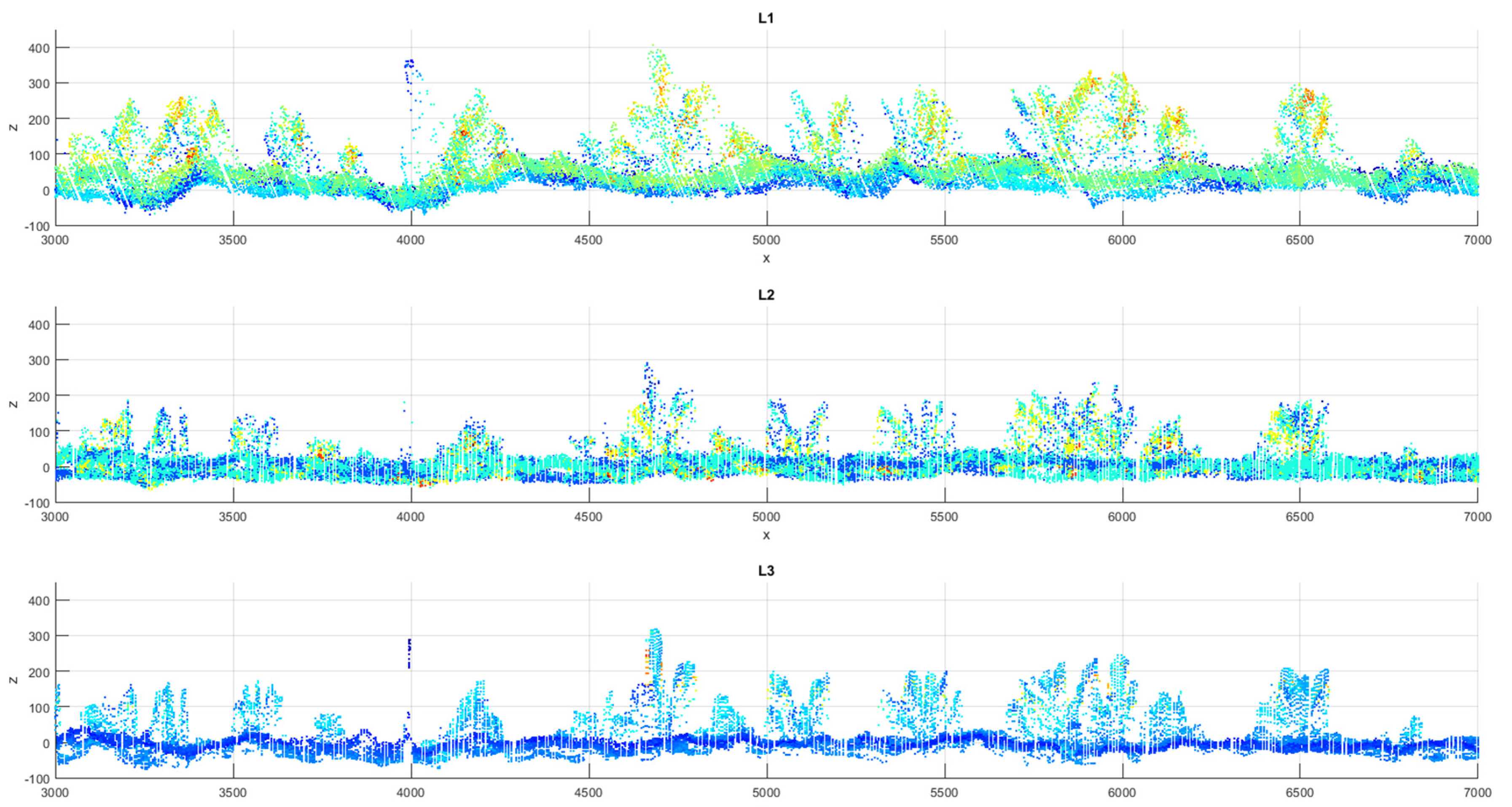
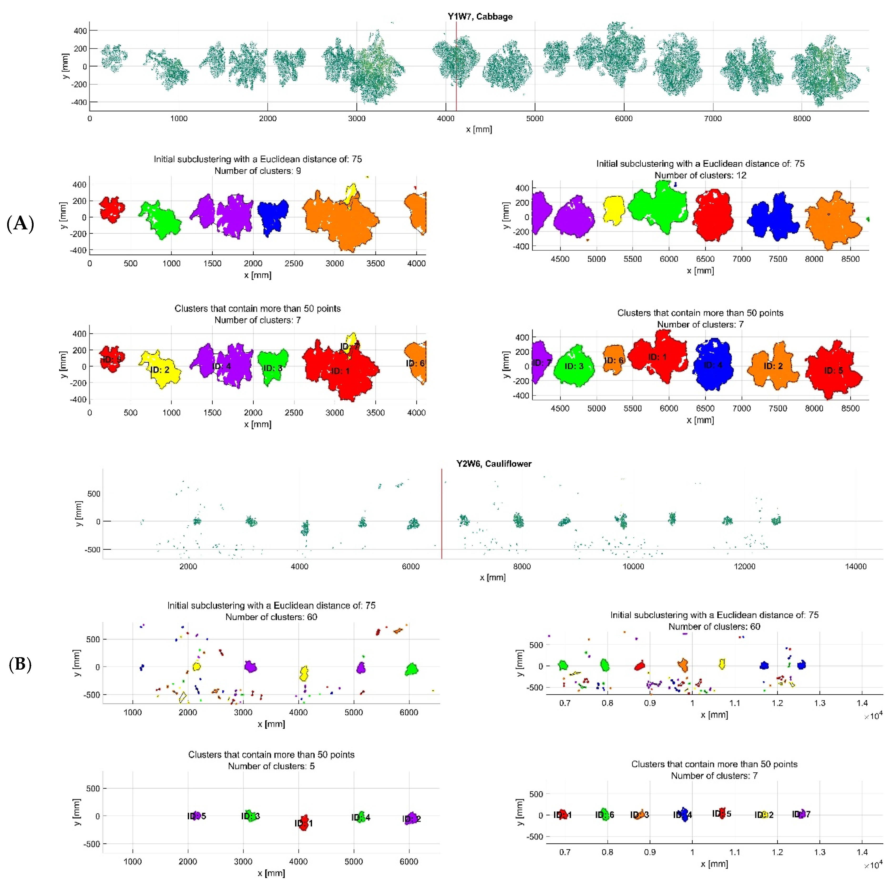
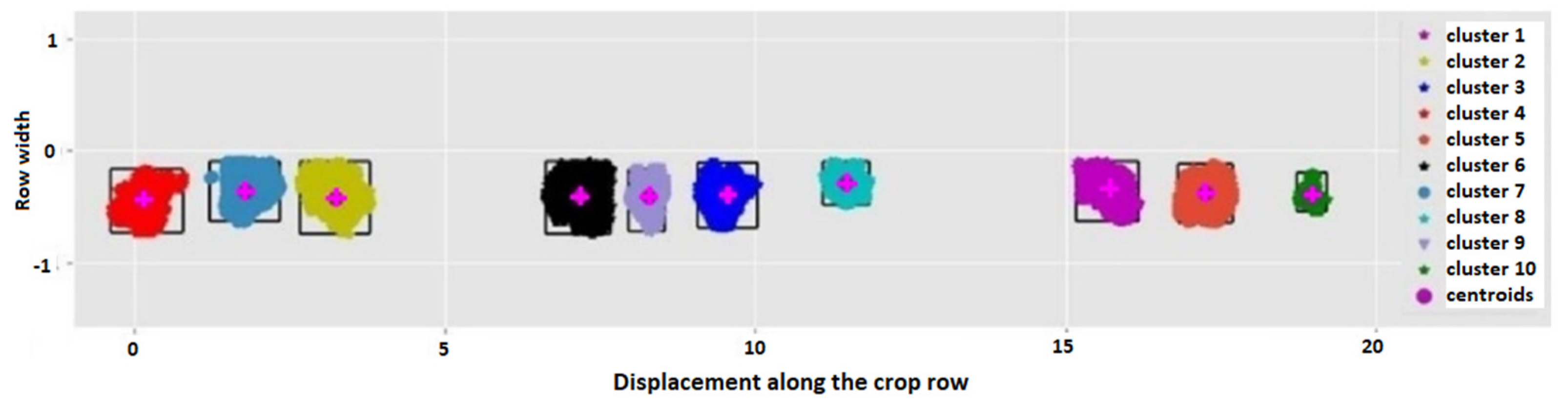
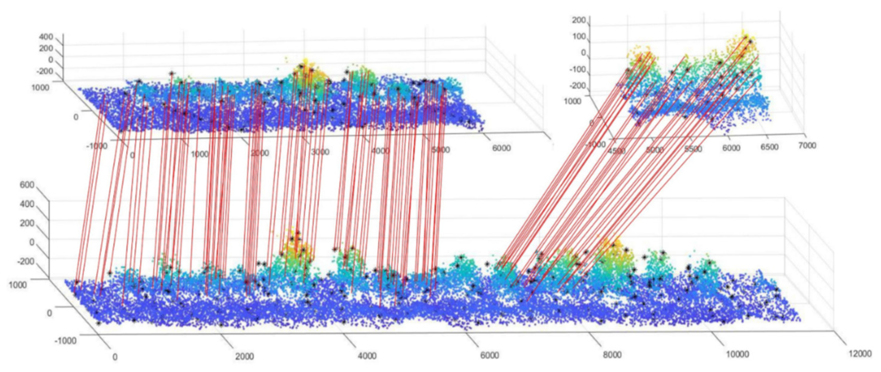
3.2. Three-Dimensional (3D) Sensing

An example of the raw data received from the three LiDARs is included in Figure 5. A stake can be seen marking the beginning of the area of interest around displacement x = 4000 and it was used to determine the translation between the different point clouds. First, the pushbroom LiDAR included in the top graph registers significantly more fluctuation in terrain compared to the other two. This could be due to the subtle changes in inclination of the lightweight cart while traveling the row, which are amplified more in the pushbroom measurement as the registered points are further away. Second, when looking at specific cabbage heads such as the ones at x = 3500 and x = 5000 in the lower graphs, a displacement to the right (in the direction of movement) can be seen in the uppermost graph, which is not present in the other cabbage heads or the wooden stake. Third, the wooden stake is barely detected by the vertical LiDAR, which can be explained by the stake aligning with the laser beam in that orientation. Finally, the vertical and lateral LiDAR will suffer gaps or cart inclinations while scanning the same cabbage, whereas the pushbroom LiDAR will be looking ahead to the upcoming crops, which explains the near perfect alignment in the lower two graphs.
As no colour or spectral information is retained, only three-dimensional information is present in this type of point cloud, so the points needed to be identified as crop or non-crop purely based on their location and height. Especially for smaller plants, the coarseness of the terrain yields height data that are comparable to the height data of lower hanging leaves. This means that an identification based on only height data was not possible.
To overcome this, each point was assigned a value J based on the heights of all points within a 150 mm radius, where the closest points are considered more heavily than those at the border of this sphere. The resulting value is averaged over the number of points, as this yields a higher contrast in the histogram of all values of J, i.e., J is an averaged sum of height squared over distance. The number of points that are present within this radius varies as some areas are detected by multiple LiDAR devices, whereas other areas only have a direct line of sight, for example the low-mounted lateral LiDAR. Equidistant sampling of the merged point clouds at 1.5 cm intervals resolves this imbalance, while also reducing the calculation time of the averaged sum.
Based on the histogram of all J values of the downsampled merged point cloud several properties can be automatically detected, such as steepest decline in the bin count as proposed in [23]. This histogram edge is close to the upper edge of the naturally distributed J values of the soil points, but results in a conservative estimation of the soil. However, through Otsu’s method, the vegetation cloud estimation was too conservative. Thus, the local minimum of the J histogram with the highest prominence value, bounded by these lower and upper limits, yielded the best bisection of the point cloud into vegetation and soil throughout different stages of the growing season, as assessed visually.
Points with a value of J higher than this threshold value, the previously described local minimum, are considered plant points, and lower values are considered non-plant matter. This algorithm allows low leaves and protruding surfaces such as rocks to be identified correctly, despite the rock points possibly having higher altitude values than those of the low leaf, as shown in Figure 6.
The resulting merged 3D point cloud containing only plant points can subsequently be cleaned, where any singular noise points are removed. Then, a clustering procedure is applied on the point clouds using a Euclidean distance of 75 points, in order to singularize and label each single plant. Examples of these results are shown in Figure 7A,B, for a row of cabbages and cauliflowers, respectively. The western half (left) of the row was fertilized less than the eastern half (right) prior to the establishment of the plant.
For each of the identified clusters, a range of characteristics was calculated: surface area of covered soil, height, cluster volume, cluster surface to volume ratio, and distribution of J values. These metrics were compared between crops that had received different fertilizer doses and were combined later with VI data to decide on single-plant fertilization.
As a validation of results, reference data from plant heights was compared with LiDAR data. Identification of where in the cluster one crop finishes and the other starts was not always possible, especially for the larger crops in the second half of the growing season. Crop centers were estimated based on the shape of the cluster and continuity between measurements. For cauliflower, the amount of manually documented heights was consistent from week to week, and the comparison between manual and 3D cluster heights is included in Figure 8. Each measurement is represented by a colour of increasing intensity and contains 19 data points, where green and blue indicate the first and second seasons, respectively. The correlation reached an R of 0.8; the shift from the perfect correlation can be explained by a tendency to overestimation using a ruler or by a local elevation in soil height that is not taken into account when estimating the cluster height.
The evolution of the two aforementioned vegetation metrics over time is included in Figure 9 for red cabbages, along with a visualization of the definition of both metrics: cluster volume and covered soil surface. These values represent the total of all clusters with the same fertilization strategy, after filtering for cluster size as explained in the previous section. This yields two quantifiable measures per crop type per half of the field. The 13 red cabbage measurements collected during the weeks after transplantation (WAT) (noted W1, W2, etc. in the figure) illustrate the volatility of the volume metric, with respect to the projected surface coverage. Along the 42 measurements, the volume of the eastern half is less than the volume in the western half for only five measurements, 2 of which are in cabbages in the second season. In the second season, the vegetation and, therefore, the clusters are smaller than anywhere in the first season, and the values of both field halves lie very close together in all of the measurements of that year. For the less erratic soil surface area, 4 of the 42 measurements indicate that the covered surface is smaller on the eastern half than on the western half, 3 of which are in the second, less reliable, season. The poor relation among pre-crop fertilization and plant development in the western/eastern part of the field could be due to several causes, such as irregular soil profile, local differences is soil nutrition or individual plat stress. However, single plant volumes and projected surfaces can be satisfactorily tracked during crop development.
In Figure 10 the total volumes of vegetation per running meter per fertilization strategy are shown for three types of crops. Here, the yellow lines correspond to the solid lines in Figure 9. The relative size and thus the significance of the results of the second season can clearly be seen in contrast to the first season, as the crops were transplanted late and removed prematurely, as a plague of rabbits invaded the field. The difference between fertilization strategies is consistently registered from about 3 WAT onward.

3.3. Combination of Multi-Spectral and Three-Dimensional Analysis

The identified vegetation based on the data of both types of sensors can be compared through their surface area, using the projected area of the three-dimensional vegetation point clouds onto the horizontal plane. The resulting areas of several crop rows with varying fertilization dosage, measured throughout two growing seasons, showed great consistency between each of the sensor results, yielding an R2 of 0.88.
The multispectral sensing algorithm is able to detect any individual plant with either delayed size in terms of covered soil or altered vegetation index values. The 3D sensing algorithm also identifies delayed development in terms of volume or height. This means that a combination of both sensors was preferred to determine the fertilisation necessity of individual plants. This fertilisation necessity was translated into a binary prescription map, where each individual plant in need of additional fertilisation was marked prior to application. A detailed description of the decision-making algorithm and how it was implemented in the robotic actuator control system can be found in [24].
Besides this prescription map, the data of the 3D algorithm was used as a reference world model for the actuation algorithms, which serves both to locate the cart in the field and to plan the movements of the robotic arm as discussed below.
The drawbacks and potential pitfalls of these algorithms are the detectability of newly transplanted crops (under 5 cm of height), as both sensors and would not be treated. As the field is prepared prior to transplantation and all individuals will need fertilizer, this does not pose a large problem. The distance between plants is another aspect that should be considered, as plants that overlap cannot be separated by either of the proposed sensing algorithms. This should be taken into account when assessing the results once the plants reach a certain growth stage where this starts to occur. Finally, the algorithms now assume all plant matter to belong to desired crops; in other words weeds could mistakenly be identified as individuals with a delayed development when compared to the plants of the desired crop in that row. Crop-type identification can be added to these algorithms in the future, but was not considered in this proof of concept.

3.4. Actuation

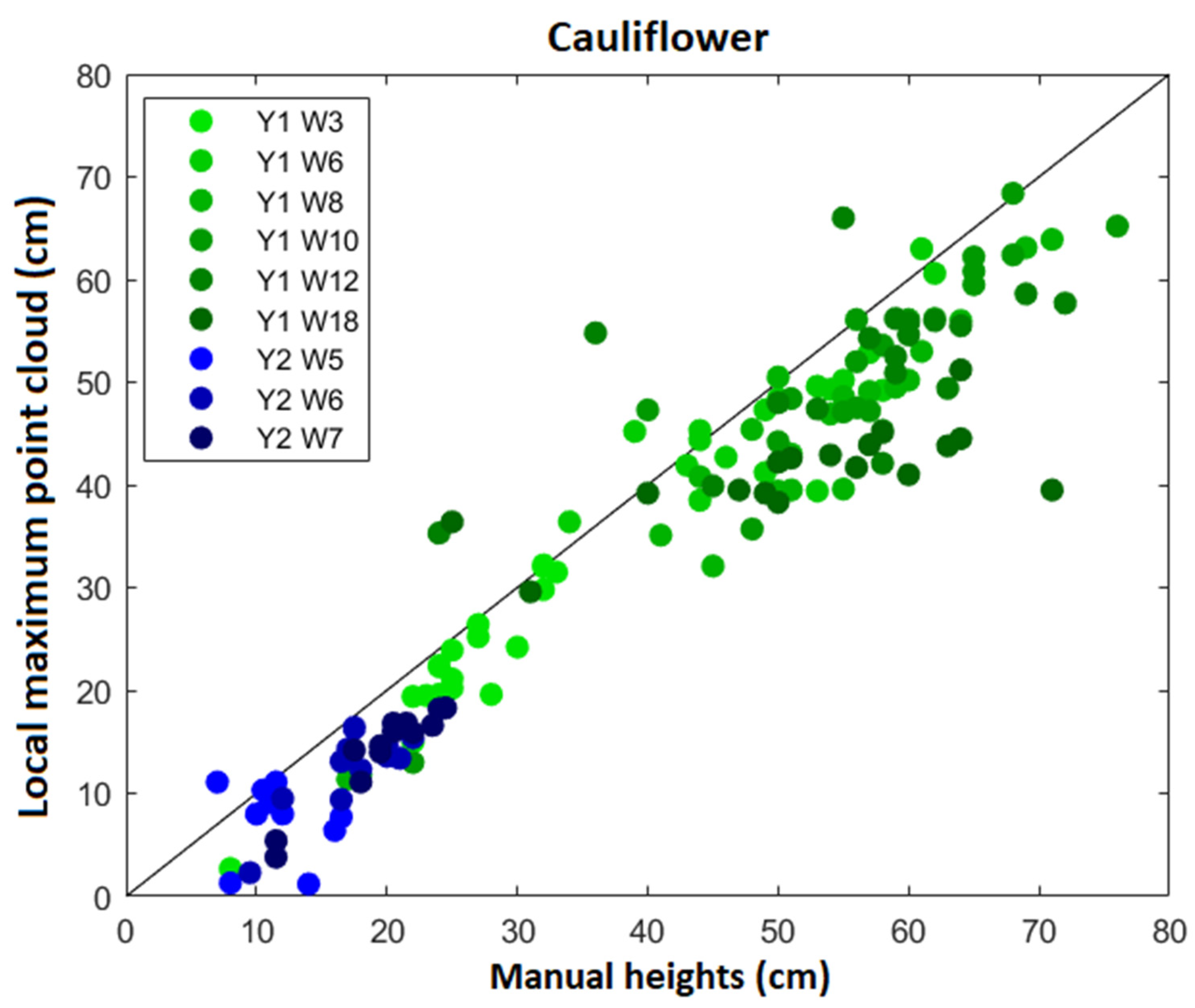
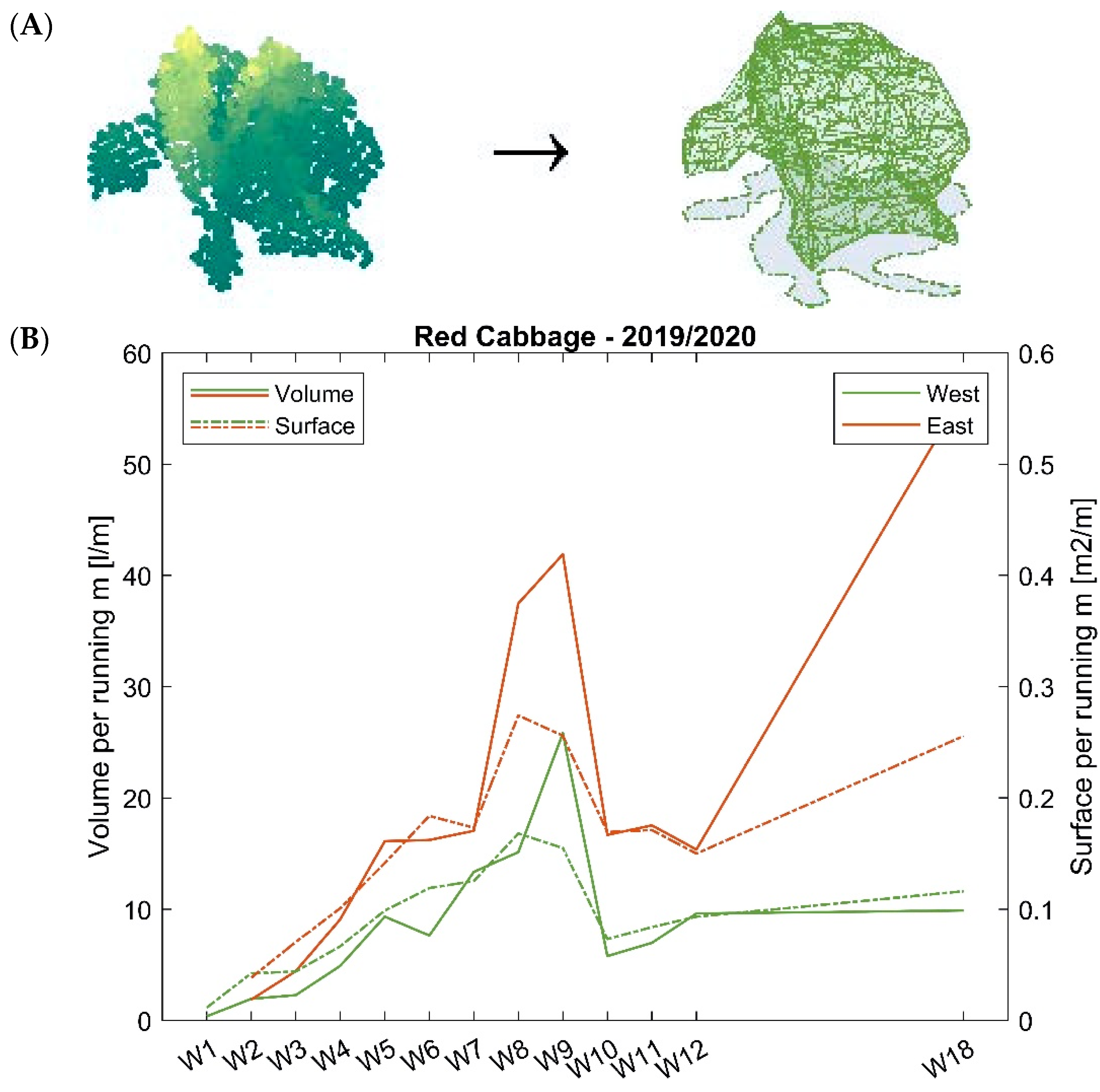
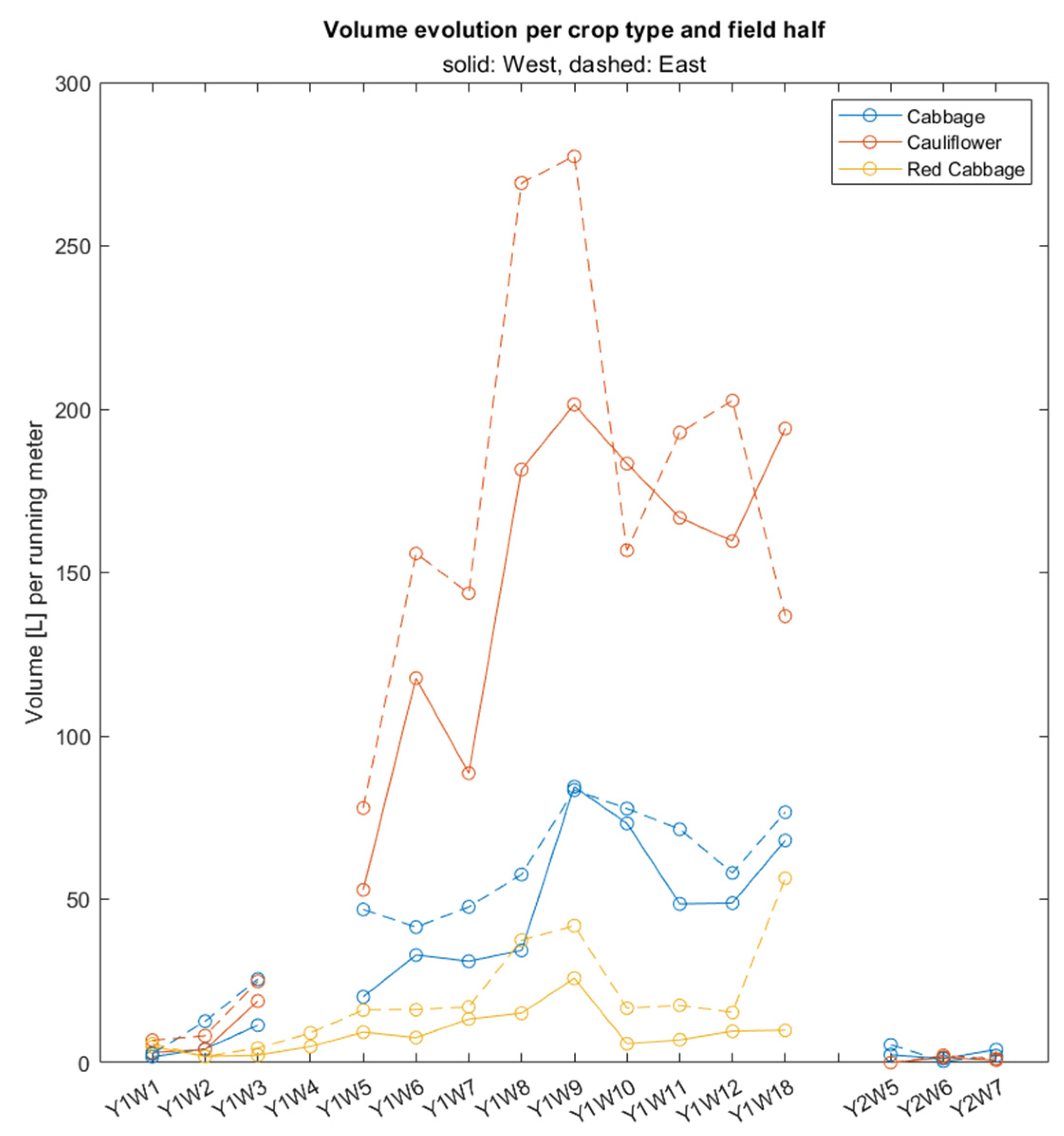
3.4.1. Geometrical Characterisation
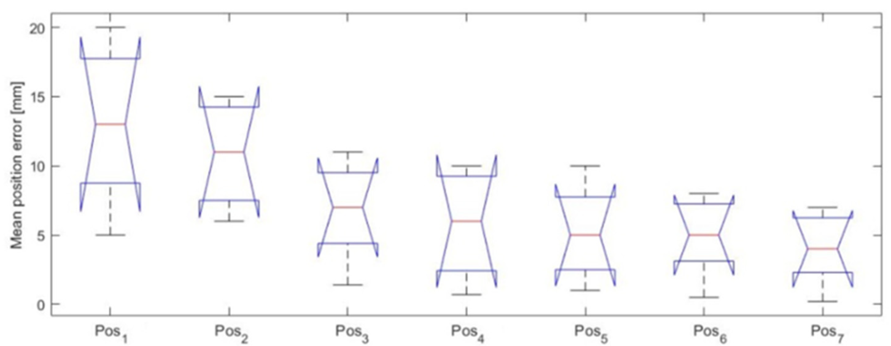
The clusters extracted in the previous section served as a reference to establish a path for the movements of the robotic arm to apply the liquid treatment. The parameters extracted are shown in Figure 11 in the form of centers and defined edges. Colours indicate each identified group. For the processing of the clusters, the unsupervised learning process K-means has been used, where the clusters are grouped with labels “cluster 1–10”.

3.4.2. Localisation

One of the essential aspects during the application of fertiliser with the robotic arm was to locate the robotic platform within the crop at all times without using an external positioning device (such as GPS) or any reference markers. The developed method takes the previously developed point cloud, captured with 3 LiDAR devices, creating a G-PC (Global Point Cloud) as well as a second real-time cloud L-PC (Local Point Cloud) of only 1 LiDAR, concerning the sections of G-PC that the platform reads while moving forward (being initially small).
In Figure 12 the correspondence of L-PC points with G-PC points is indicated with red lines for two examples of L-PCs of different sizes. This establishes the position of the local cloud within the known environment and the position of the robotic platform within the crop row.
Figure 13 shows the perception system (G-PC and robot visualisation), where the point cloud and the estimated position of the platform are shown for each instance. As the robotic platform progresses from point 1 to point 7, the L-PC accumulates earlier values, continuously improves the location estimation.
In Figure 14, a box plot shows the decreasing localisation error found at each of the positions indicated in Figure 13. Initially, the average error was around 12 mm; which reduces to approximately 0.1% at the end of a row.
This initial positioning error did not affect the fertilization, because a 5 cm was added to the radius defined in the extraction of geometric parameters extraction to encompass the plant and define the passage zone of the arm trajectory, thus avoiding the application of the fertiliser directly on the plant and damaging it. As the platform progresses, new points are added to the L-PC, allowing for more key points and improved localisation, resulting in errors with an average of 5 mm.

4. Conclusions

A proof-of-concept prototype was built, as a sensing system composed of LiDAR sensors, a multispectral camera mounted on a mobile platform equipped with an odometry sensor, and an actuation system based on a robotic arm and a pumping system for liquid fertiliser attached to the same platform. The sensing system gathers information from the plants in the row about crop volume (LiDAR), crop health (multispectral images), and plant position (point cloud for navigation). Then a decision about the need for fertilization (yes/no) is made and the actuation system applies liquid fertiliser to the soil around the plant avoiding contact with the crop.
Algorithms created for plant detection are able to identify correctly single plants and to perform calculations on them, such as NDVI of foliar surfaces and morphological measurements (plant volume, height, soil surface covered). The validation of manually measured plant heights reached R = 0.8. At the beginning of the crop season, the newly transplanted crops provide very little height difference when compared to the coarseness of the soil, which is why when plant height is below 5 cm, only the use of the multispectral algorithms is recommended. On the other hand, at the end of the season, when the leaves overlap, the actual algorithms fail to separate individual plants, and this must be solved in future research. Regarding the location of the platform, even though it was operated manually, the developed algorithm was able to recognize the three-dimensional models constructed using data from previous passes to calculate the exact position of the platform, and to plan and execute the fertiliser application without damaging the plants. Localisation errors ranged from 15 mm at the beginning of each row and converged rapidly to less than 5 mm.
From a proof-of-concept point of view, the proposed objectives were met, as singled plants were located and characterized, and fertilization actuation was carried out on targeted specimens.
Future work includes expansion of this research to other (strip-cropping) vegetable crops, comparing these results with other sensors, and expanding the research from fertilization needs to other interventions, e.g., pest detection and mitigation.

Author Contributions

Conceptualization, C.V., A.B., A.K., C.C.U. and J.d.C.; methodology, J.J.R.-M., P.G., A.B. and C.V.; software, A.K. and C.C.U.; validation, A.K. and C.C.U.; formal analysis, A.K. and C.C.U.; investigation, A.B., C.V., A.K., C.C.U. and J.d.C.; resources, J.J.R.-M., P.G., C.V. and A.B.; data curation, J.J.R.-M., P.G., A.K. and C.C.U.; writing—original draft preparation, A.K., C.C.U. and C.V.; writing—review and editing, A.K., C.C.U., C.V. and A.B.; visualization, C.V. and A.B.; supervision, C.V. and A.B.; project administration, C.V., A.B. and J.d.C.; funding acquisition, C.V. and A.B. All authors have read and agreed to the published version of the manuscript.

Funding

This research has been possible thanks to the financing of the European project “Sureveg: Strip-cropping and recycling for biodiverse and resource-efficient intensive vegetable production”, belonging to the action ERA-net CORE Organic Cofund: http://projects.au.dk/coreorganiccofund/ by the two national projects AEI (Agencia Estatal de Investigación) PCI2018-093074 and PCI2018-093046, corresponding to call MCIN/AEI/10.13039/501100011033/. Also thanks to RoboCity2030-DIH-CM, Madrid Robotics Digital Innovation Hub, S2018/NMT-4331, funded by “Programas de Actividades I+D en la Comunidad Madrid” and cofunded by Structural Funds of the EU.

Acknowledgments

This work was accomplished thanks to the support of: ERAnet CORE Organic Cofound—Sureveg Project, AEI (Agencia Estatal de Investigación), CSIC (Consejo Superior de Investigaciones Científicas), CAR (Centro de Automática y Robótica), and Departamento de Ingeniería Agroforestal, ETSI Agronómica, Alimentaria y de Biosistemas, Universidad Politécnica de Madrid. Authors would like also to thank the colleagues at UPM who helped and supported building the prototype, managing the crops, gathering experimental data and discussing data modelling along the different seasons, as well as to all the partners in the SUREVEG project.

Conflicts of Interest

The authors declare no conflict of interest. The funders had no role in the design of the study; in the collection, analyses, or interpretation of data; in the writing of the manuscript, or in the decision to publish the results.

References

  1. Ritson, C. Population Growth and Global Food Supplies. In Food Education and Food Technology in School Curricula 2020; Springer: Cham, Switzerland, 2020; pp. 261–271. [Google Scholar]
  2. Pachapur, P.K.; Pachapur, V.L.; Brar, S.K.; Galvez, R.; Le Bihan, Y.; Surampalli, R.Y. Food Security and Sustainability. Sustainability: Fundamentals and Applications; Surampalli, R., Zhang, T., Goyal, M.K., Brar, S., Tyagi, R., Eds.; John Wiley & Sons, Ltd.: Hoboken, NJ, USA, 2020; pp. 357–374. [Google Scholar]
  3. Srivastava, R.K. Influence of Sustainable Agricultural Practices on Healthy Food Cultivation. In Environmental Chemistry for a Sustainable World; Springer: Cham, Switzerland, 2020; pp. 95–124. [Google Scholar]
  4. Loures, L.; Chamizo, A.; Ferreira, P.; Loures, A.; Castanho, R.; Panagopoulos, T. Assessing the effectiveness of precision agriculture management systems in mediterranean small farms. Sustainability 2020, 12, 3765. [Google Scholar] [CrossRef]
  5. Poblete-Echeverría, C.; Fuentes, S. Editorial: Special issue “Emerging sensor technology in agriculture”. Sensors 2020, 20, 3827. [Google Scholar] [CrossRef] [PubMed]
  6. Singh, R.K.; Aernouts, M.; De Meyer, M.; Weyn, M.; Berkvens, R. Leveraging LoRaWAN technology for precision agriculture in greenhouses. Sensors 2020, 20, 1827. [Google Scholar] [CrossRef] [PubMed] [Green Version]
  7. Cubero, S.; Marco-Noales, E.; Aleixos, N.; Barbé, S.; Blasco, J. Robhortic: A field robot to detect pests and diseases in horticultural crops by proximal sensing. Agriculture 2020, 10, 276. [Google Scholar] [CrossRef]
  8. Moysiadis, V.; Tsolakis, N.; Katikaridis, D.; Sørensen, C.G.; Pearson, S.; Bochtis, D. Mobile robotics in agricultural operations: A narrative review on planning aspects. Appl. Sci. 2020, 10, 3453. [Google Scholar] [CrossRef]
  9. Fue, K.; Porter, W.; Barnes, E.; Rains, G. An Extensive Review of Mobile Agricultural Robotics for Field Operations: Focus on Cotton Harvesting. AgriEngineering 2020, 2, 150–174. [Google Scholar] [CrossRef] [Green Version]
  10. Hussain, M.; Naqvi, S.H.A.; Khan, S.H.; Farhan, M. An Intelligent Autonomous Robotic System for Precision Farming. In Proceedings of the 2020 3rd International Conference on Intelligent Autonomous Systems, ICoIAS 2020, Singapore, 26–29 February 2020; Institute of Electrical and Electronics Engineers Inc.: New York, NY, USA, 2020; pp. 133–139. [Google Scholar]
  11. CORE Organic Cofund. Available online: http://projects.au.dk/coreorganiccofund/research-projects/sureveg/ (accessed on 3 March 2019).
  12. Hajjaj, S.S.H.; Sahari, K.S.M. Ieee Review of Agriculture Robotics: Practicality and Feasibility. In Proceedings of the IEEE International Symposium on Robotics and Intelligent Sensors (IRIS), Tokyo, Japan, 17–20 December 2016; pp. 194–198. [Google Scholar]
  13. Vougioukas, S.G. Agricultural robotics. Annu. Rev. Control Robot. Auton. Syst. 2019, 2, 365–392. [Google Scholar] [CrossRef]
  14. Fountas, S.; Mylonas, N.; Malounas, I.; Rodias, E.; Hellmann Santos, C.; Pekkeriet, E. Agricultural Robotics for Field Operations. Sensors 2020, 20, 2672. [Google Scholar] [CrossRef] [PubMed]
  15. Barbosa, W.S.; Oliveira, A.I.S.; Barbosa, G.B.P.; Leite, A.C.; Figueiredo, K.T.; Vellasco, M.; Caarls, W. Design and Development of an Autonomous Mobile Robot for Inspection of Soy and Cotton Crops. In Proceedings of the 12th International Conference on the Developments in eSystems Engineering (DeSE), Kazan, Russia, 7–10 October 2019; pp. 557–562. [Google Scholar]
  16. Mahmud, M.S.A.; Abidin, M.S.Z.; Mohamed, Z. Ieee Development of an Autonomous Crop Inspection Mobile Robot System. In Proceedings of the IEEE Student Conference on Research and Development (SCOReD), Kuala Lumpur, Malaysia, 13–14 December 2015; pp. 105–110. [Google Scholar]
  17. Slaughter, D.C.; Giles, D.K.; Downey, D. Autonomous robotic weed control systems: A review. Comput. Electron. Agric. 2008, 61, 63–78. [Google Scholar] [CrossRef]
  18. Gerhards, R.; Sanchez, D.A.; Hamouz, P.; Peteinatos, G.G.; Christensen, S.; Fernandez-Quintanilla, C. Advances in site-specific weed management in agriculture-A review. Weed Res. 2022, 62, 123–133. [Google Scholar] [CrossRef]
  19. Kumar, P.; Ashok, G. Design and fabrication of smart seed sowing robot. In Proceedings of the 3rd International Conference on Advanced Materials and Modern Manufacturing (ICAMMM), Chennai, India, 3–4 April 2020; pp. 354–358. [Google Scholar]
  20. Aravind, K.R.; Raja, P.; Perez-Ruiz, M. Task-based agricultural mobile robots in arable farming: A review. Span. J. Agric. Res. 2017, 15, e02R01. [Google Scholar] [CrossRef]
  21. Wang, Z.H.; Xun, Y.; Wang, Y.K.; Yang, Q.H. Review of smart robots for fruit and vegetable picking in agriculture. Int. J. Agric. Biol. Eng. 2022, 15, 33–54. [Google Scholar]
  22. Ditzler, L.; Driessen, C. Automating Agroecology: How to Design a Farming Robot Without a Monocultural Mindset? J. Agric. Environ. Ethics 2022, 35, 2. [Google Scholar] [CrossRef] [PubMed]
  23. Jiang, Y.; Li, C.; Takeda, F.; Kramer, E.A.; Ashrafi, H.; Hunter, J. 3D point cloud data to quantitatively characterize size and shape of shrub crops. Hortic. Res. 2019, 6, 43. [Google Scholar] [CrossRef] [PubMed] [Green Version]
  24. Cruz Ulloa, C.; Krus, A.; Torres Llerena, G.; Barrientos, A.; Del Cerro, J.; Valero, C. ROBOFERT: Human-Robot Advanced Interface for Robotic Fertilization Process. In Trends in Artificial Intelligence and Computer Engineering; Botto-Tobar, M., Gómez, O.S., Rosero Miranda, R., Díaz Cadena, A., Montes León, S., Luna-Encalada, W., Eds.; ICAETT 2021; Lecture Notes in Networks and Systems; Springer: Cham, Switzerland, 2022. [Google Scholar] [CrossRef]
Figure 1. Frontal view (b) and rear of the platform (a), the yellow circles show the 3 LiDAR sensors and the red circle indicates the multispectral camera.
Agronomy 12 01339 g001
Figure 2. Robotic fertilization prototype in the cultivation row. Red: tank with liquid treatment, yellow: nozzle.
Agronomy 12 01339 g002
Figure 3. Distribution of NDVI values in a cabbage row, and its correspondence with histogram information.
Agronomy 12 01339 g003
Figure 4. NDVI values and their histogram distribution after applying a Gaussian filter. In red, the local minimum between soil and vegetation as identified by Otsu’s method.
Agronomy 12 01339 g004
Figure 5. Lateral view of part of a cabbage strip, with L1 (top) denoting the pushbroom LiDAR, L2 (middle) showing the vertical LiDAR data, and L3 (bottom) the lateral LiDAR mounted near the right front wheel. Colour denotes the reflectance value as registered by the LiDARs.
Agronomy 12 01339 g005
Figure 6. The point cloud with colour denoting height data (left) alongside the same cloud coloured by the values of the function J.
Agronomy 12 01339 g006
Figure 7. Example of a cabbage row in the middle of the first season (Part (A)) and a cauliflower row at the start of the second season (Part (B)). Depicted are the points of the downsampled merged point cloud that exceed the defined threshold value of J (above), clusters based on Euclidean distance (middle), cleaned and labelled (bottom). The western half (left) is fertilised less than the eastern half (right).
Agronomy 12 01339 g007
Figure 8. Correlation between manual height measurements of each crop and the maximal point cloud height of all 19 cauliflower in season 1 and 16 cauliflowers in season 2, coloured by date.
Agronomy 12 01339 g008
Figure 9. (A) Example of a cabbage cluster based on LiDAR data (left) alongside the definition of its volume (solid green) and projected soil surface (shaded area with dash dotted green border). (B) The same green lines are used to indicate the total of all cluster volumes (solid, left y-axis) and surfaces (dash dotted, right y-axis) of the eastern (green) and western (red) field half over time.
Agronomy 12 01339 g009
Figure 10. Volume evolution per crop type and field half. The yellow lines (red cabbage) coincide with the solid lines (volume) in Figure 9. The eastern half (dashed) received more fertiliser than the western half (solid), across all crop types.
Agronomy 12 01339 g010
Figure 11. K-means classification and geometrical parameters extraction from a row crop.
Agronomy 12 01339 g011
Figure 12. Matching key points from the L-PC ((upper)—two captured partial sections) to the G-PC (lower).
Agronomy 12 01339 g012
Figure 13. Mobile robotics platform position and data visualisation as simulated using rviz framework. Numbers (1–7) denote subsequent detections of single plants.
Agronomy 12 01339 g013
Figure 14. Box diagram of mean localisation errors at each of the cart positions indicated in Figure 13, while the platform was moving over the crop row.
Agronomy 12 01339 g014
Publisher’s Note: MDPI stays neutral with regard to jurisdictional claims in published maps and institutional affiliations.

