Nitrogen Hotspots on the Farm—A Practice-Oriented Approach

Abstract

The proactive management of nitrogen (N) on a farm is the best way to protect the environment against N pollution. The farm is the basic business unit, where simple and low-cost methods of identifying and ameliorating weaknesses (nitrogen hotspots) in the N-flow chain can be applied. The basis for the effective use of mineral N fertilizers (N_f) is the farmer’s knowledge of the farm’s own N resources, their quantity, and the potential availability for growing crops. These resources include both primary sources of N (N₂ fixed by legumes) and those that are recyclable, which include crop byproducts and manure. On the other hand, crop requirements must be accurately quantified to exploit the yield potential of the crop varieties grown on the farm. The basic challenge for the farmer is to maximize the use efficiency of the N resources. In this regard, the farmer has two diagnostic tools available to recognize nitrogen hotspots and to quantify N resources. These are (1) the N balance method (difference between the N inputs and outputs), which allows for a surplus or deficiencies in the N-flow between farm units (fields, livestock housing) to be identified, and (2) the nitrogen gap, which is based on the amount of N_f applied and the yield of a given crop. It is possible to calculate the maximum attainable yield as well as identify the fields on the farm that require a correction of N management.

1. Introduction—Food Gap and Sustainable Agriculture

Any calculation of future food demand must take into account at least two driving forces. The first (and dominant) is the global population, which is projected to reach 9.7 billion in 2050 [1]. The second driver is the change in consumption patterns. According to Engel’s law, household income is primarily spent on animal products, mainly meat and dairy, regardless of the wealth of a country [2]. For these reasons, the food demand projections for 2050 are about 70% above the 2014 level [3,4].

Food economy experts have discussed a number of global solutions to try to find a balance between the constantly growing demand for food and the pressure of agricultural production on the environment [5,6]. Two main strategies have been posited to cover the food gap: consumption- and production-oriented. The former is based on the assumption that the current level of food production is sufficiently high to cover the food gap, provided that food waste is significantly reduced or even eliminated. A sharp decline in the consumption of meat, and even dairy products, forms only a part of a broader scientific discussion, which also applies to dietary changes as a way to decrease the food gap [6,7,8]. The second main strategy assumes a significant increase in crop and animal production [9]. However, the need to increase the crop production results not only from the demand for food, but also from the projected increase in the demand for non-agricultural plant products such as bio-oil, bioethanol, or industrial starch [10,11].

In general, two approaches to increase food production have been considered. The first approach is essentially intensive, namely, to increase yields by the effective use of fertilizers, pesticides, and fuel. The second is essentially extensive, which occurs through the expansion of agricultural land. The perceived negative aspects of the latter result from (i) a lack of fertile soils, and (ii) the need to use large resources to achieve the optimal level of new arable land productivity [12,13]. Two irreversible effects of the current ways of food production on the environment are discussed. The first is the direct impact of the food system, regardless of the field location, on both the local and global environments [11]. The second is largely based on the exploitation of non-renewable resources. The success of the Green Revolution would not have been achieved without intensive production measures, mainly nitrogen fertilizers (N_f) and agrochemicals, to protect crops from the pressure of weeds, pathogens, and insects [14]. However, the intensive use of N_f has posed a threat to both the local and global environments [15].

The reduction in the food gap by 2050 requires the implementation of complementary strategies. The most important aspects of this assumption are: (i) a yield increase in the main staple crops; (ii) an increase in the area of arable land; and (iii) a decrease in food waste. The first strategy will be difficult to achieve because the annual rates of the yield increase in staple crops such as wheat, maize, rice, and soybean are far below the 2.4% target [16]. This simply means that it will only be possible to cover the yield gap if certain non-agricultural ecosystems are converted into arable land. It is necessary to emphasize that a greater consumption of N_f should be consistent with the main assumption of the sustainable intensification of agriculture approach. The essence of this concept is to increase food production per unit of the applied measure while maintaining the health of local and global ecosystems [17,18,19].

The use of new crop varieties can be effective, provided that a well-developed N_f application strategy is in place. However, it should be noted that both water and N are not complementary means of production, but instead interact with each other. The main challenge for both researchers and farmers is the sustainable use of these resources, which in turn depends on the optimization of the other production factors [20,21,22].

Environment pollution caused by the dispersion of active N compounds from farms to the surrounding ecosystems has become a serious societal problem over the last 40 years [23]. In the public awareness, this threat has become a key environmental issue; a dangerous byproduct of agricultural practice [24]. The EU Nitrates Directive confirms the severity of N pollution [25]. As such, the efficient management N on the farm is crucial for crop yields (as a key component of farm incomes) and environmental health [26]. The pro-production activity of the farmer requires the efficient use of all N resources on the farm, purchased as either N_f or obtained from its recycling. The N hotspots on the farm are those N resources, which if skillfully managed, can have a serious and positive effect on both the crop production and the environment. Three N hotspot groups on the farm require careful management by the farmer and are of major importance in terms of crop production and environmental protection. First, the synchronization of the N demand and supply to the growing crop [27]. To meet the demand of the plant for N requires the maximum exploitation of the soil resources (mineral N pools) and the effective use of N fertilizers [28]. Legumes that fix atmospheric N₂ must be included in N budgeting on the farm [29]. The second group includes the different types of organic amendments. Recycled N resources such as manure, slurry, and digestate are chemically highly labile due to a high ammonium content [30]. The transformation of ammonium into ammonia results in volatilization to the atmosphere and is a loss of a nutrient that is necessary for crop production as well as an environmental problem [31]. The third group includes crop residues (CRs), which are both a source of organic matter and, depending on the N content, an effective means of post-harvest, residual N_min control [32]. A key challenge for the farmer is to determine how to manage N on the farm in the most sustainable way. The objective of this review was to analyze the current state of N-flows on the farm to identify potential Nitrogen hotspots in N management. This conceptual review also highlights a number of practical solutions that a farmer can implement without increasing the production costs.

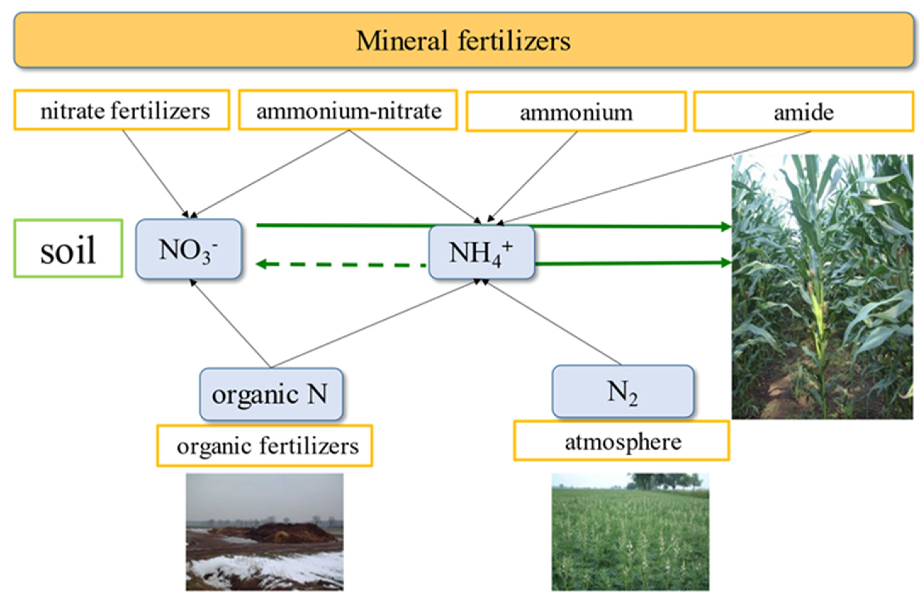
2. Nitrogen Sources

2.1. Simplified Diagram of the N Cycle on the Farm

There are numerous models or diagrams that present the N cycle at varying levels of complexity. The most advanced models show and quantify the intended and unintended N-flow pathways between the soil/plant system and adjacent environments including both the atmosphere and water [33,34]. For a farmer, the most important set of required data concerns those N pools that can be quantified on the farm. This should be a basis from which to determine the amount of N to be purchased as fertilizer. The first key resource is the N pool that is in the soil (Figure 1). Plants take up N in its inorganic forms (i.e., nitrate (N-NO₃) and ammonium (N-NH₄)), which are the end products of a series of N transformation processes:

N₂ → N_org → NH₄⁺ → NO₃⁻

(1)

The total potentially available N (mineral N, N_min = N-NH₄ + N-NO₃) consists of three sub-pools: (i) N_min present in the soil at the beginning of the growing season; (ii) N applied as N_f and/or as manure; and (iii) the available N released from soil resources during the growing season [35,36]. In farming practices, the N_min pool is determined before sowing/planting or at the beginning of the growing season of winter crops [37,38]. One exception is maize, where N_min is also determined at the fifth leaf stage, which is considered as the cardinal knot of yield formation in that crop [35]. The N_f is the only N pool that is actually known (i.e., strictly defined by the farmer) [39].

The natural, primary source of inorganic N in the soil, and thus the farm’s own N resource is atmospheric N₂ fixed by microorganisms alone or in collaboration with higher plants in a series of processes known as biological nitrogen fixation (BNF) [40]. Secondary sources of N for crops are organic N compounds, which are then transformed by microorganisms into plant available forms [41].

2.2. Biological Nitrogen Fixation (BNF)—The Primary Source of N for Plants

The functions of N including food production should be regarded as the results of a series of seemingly mutually exclusive phenomena. The basic source of N for all living organisms on Earth is the atmosphere, in which 78% of the total gas content is N₂. This molecule is chemically inert [42,43].

The conditions necessary for the successful exploitation of atmospheric N₂ is the presence of strictly defined groups of microorganisms and compatible plant species. The reduction of N₂ in nature can only be performed by prokaryotic organisms equipped with the enzyme nitrogenase. This enzyme consists of two proteins: dinitrogenase reductase (a Fe-protein) and dinitrogenase (a Mo-Fe-protein). Moreover, the reaction can only be effective when the plant is well nourished with phosphorus (P) and magnesium (Mg). For a farmer who cultivates legumes, it is imperative that elevated levels of these nutrients are maintained in the soil due to the high energy costs associated with N₂ incorporation into a legume plant [44].

Among the microorganisms that carry out BNF, two groups can be distinguished. The first is represented by free-living N₂ bacteria (Azotobacter sp., Azospirillum sp., Bacillus sp., Beijerinckia sp., Clostridium sp., and some others) as well as photosynthetic bacteria (Rhodobacter sp.). This group also includes cyanobacteria—Anabarna sp., which is present in both soil and water reservoirs. The second group consists of symbiotic bacteria representing the Rhizobiaceae genus, which are able to fix N₂ through symbiosis with plants from the Fabaceae family. The symbiosis of these bacteria with the plant is based on the formation of a nodule on the plant root, in which the microorganisms reduce N₂ by using the energy compounds from the plant for this process [45,46].

Biological nitrogen fixation is a basic process that forms the platform for the synthesis of all other N compounds including those responsible for the absorption of inorganic N ions from the soil solution. The energy costs of N₂ fixation by plants in symbiosis with microorganisms result from (1) the reduction of N₂ to NH₃; (2) transport of the carbon skeletons from the leaves to roots; and (3) the transport of amino-acids from the roots to the leaves. In comparison, it is at least 12-times greater than that required for nitrate ion absorption [42].

The symbiosis between the plant (host) and bacteria is both complex and is a multi-stage process. It begins with the mutual recognition of both partners (chemotaxis). Legume species show a strictly defined relationship to the genotype of bacteria (

Table 1. The basic symbiotic pairs in agriculture [50,51,52].

Genus/Bacteria Species	Plant Species
Rhizobium leguminosarum biovar viciae	Pisum, Viciae, Lathyrus, Lens
Rhizobium trifolii	Trifolium
Rhizobium phaseoli	Phaseolus
Sinorhizobium meliloti	Medicago, Melilotus, Trigonella
Bradyrhizobium sp.	Glycine
Bradyrhizobium japonicum	Lupinus

). In the legume, BNF starts with the secretion of a mixture of compounds containing betaines, flavonoids, and izoflavonoids into the rhizosphere. These plant specific signals are picked up by bacteria that activate a set of genes called Nod factors. These genes trigger the production of the oligosaccharides necessary for the infection of the plant root, specifically the root hair. The size and shape of the bacteria nodule (bacteroid) depends much more on the plant species than on the bacteria genotype [47,48]. The yield from BNF (i.e., the amount of fixed N₂, varies with the growth stage of the legume plant). It reaches a maximum before plant flowering and the decline in N₂ fixation following flowering results from the decreased carbon transport to the root, which ultimately leads to bacteroid disintegration. The main reason for this process is the emergence of a new physiological sink (i.e., the expanding seed) [49].

At the global scale, 139–170 Mt of N is introduced into the biosphere each year from BNF. Between 70–80% of this pool is formed due to symbiotic legume–bacteria associations, with the remainder (20–30%) in non-symbiotic systems. The amount of N₂ fixed by free-living microorganisms is estimated to be 0–12 kg N ha⁻¹ (

Table 2. The ranges of N fixation in various ecosystems [55], kg N ha⁻¹.

	Real Ranges	Commonly Used Ranges
Free living organisms
Forests	0–38	0–10
Rice	0–80	0–15
Symbiotic microorganisms
Azolla	10–150	10–50
Fodder legumes	15–680	50–250
Seed legumes	10–450	30–150
Legumes as catch crop	20–460	20–150
Tree/bushes legume plants	10–30	20–50

). This wide variation is due to the fact that non-symbiotic bacteria activate BNF processes only while alive, and the fixed N is only used for growth. This simply means that during the lifetime of the bacteria, N is not released to the surrounding environment and the soil is enriched in N only after the bacteria have died [53]. This N source, albeit small due to the narrow C:N ratio, can be important for crops, as has been documented for rice, for example in [23]. Moreover, due to the high efficiency of biomass production, cyanobacteria can be used as a source of raw material for bio-fertilizer production [54].

The effectiveness of nodulation, N₂ fixation, and the amount of N₂ fixed by the legume plant depends on numerous abiotic, nutritional, and biotic factors. The key environmental factors are soil humidity and temperature. Rhizobium species differ in their susceptibility to water supply. According to Zahran [56], slow-growing Rhizobia strains adopt much better to soil drought than fast-growing strains. The drying soil strongly reduces the mobility of bacteria in the soil solution, which limits the infection efficiency [57]. According to Liu et al. [40], the activity of nitrogenase for most legume species is high across a broad temperature range (12–35 °C). The optimum temperatures are, however, much narrower, in the range of 20–25 °C. Temperature regulates the root hair infection, nodule differentiation, nodule growth rate and final structure, and plant root functions. Low temperature in the early stages of root nodulation results in a smaller number and size of nodules, while excessive temperatures result in a delay to nodulation [58].

The basic soil fertility factors that significantly affect the effectiveness of N₂ fixation are pH, and the content of available nutrients such as calcium (Ca), phosphorus (P), potassium (K), Mg, sulfur (S), iron (Fe), and molybdenum (Mo) [59]. The impact of soil pH on BNF processes can be regarded through its effect on the macro- and micro-symbionts on one hand, and on the soil properties (mainly the availability of nutrients) on the other hand. Highly acidic soils (pH < 4.0) are often poor in terms of available Ca and P, and as a rule, contain high concentrations of aluminum (Al³⁺) and manganese (Mn²⁺), which are both toxic to symbionts [60]. Nevertheless, some strains of Rhizobium, for example, Rhizobium tropici, are very tolerant of soil acidity. Tolerance mechanisms are related to the glutathione content, the synthesis of which enables bacteria growth, even in extremely acidic soils. In alkaline soils (pH > 8.0), the effectiveness of N₂ fixation by legumes is also strongly reduced, mainly due to the high content of sodium chloride or carbonates [61].

On farms, the agronomic factors related to the use of N_f and the crop rotation cycles are also important for effective legume production [62]. The high content of available N in the soil/legume system negatively impacts on the processes involved in N₂ fixation. The excess of inorganic N in the soil inhibits the activity of bacterial nitrogenase [40]. This phenomenon results from the energy costs associated with inorganic N uptake from the soil by the plant, which is lower than the cost of N₂ reduction [42,44]. For this reason, when legumes are cultivated, it is recommended that the N_f rate is limited to the amount required to maintain plant growth before the beginning of the root nodule formation. If the rate is too high or is applied too late, N_f will result in weaker nodulation of the root, a slower nodule growth rate, and the inhibition of N₂ fixation [63].

A deficiency in the other previously mentioned nutrients severely limits the efficiency of BNF. This process consumes large amounts of metabolic energy in the form of adenosine triphosphate (ATP). In legumes, the P content affects the number of nodules and the activity of nitrogenase. The direct source of P for bacteria is the plant, whose nutritional status depends on the supply of available P from the soil. Moreover, the availability of P to the plant depends on the soil pH, which also determines the activity of Al, Fe, and Ca. All of these elements produce insoluble compounds when reacting with soluble P in the soil solution [55,64]. The role of Ca in BNF is two-fold. First, as a component of lime, Ca is required to regulate the soil pH, thereby indirectly affecting the availability of nutrients, especially P and Mo. Second, Ca is a key element in the formation of the nodule structure. The lack of Ca results in a smaller number of nodules per plant [65]. Magnesium and K cannot be regarded as minor nutrients for N₂ fixation by legumes, while K, together with P and Mg, are the key nutrients responsible for the transport of assimilates from the leaves to the root. Therefore, K is responsible for nodule nourishment and any deficiency leads to a reduction in nodule growth and, consequently, BNF efficiency [66]. Micronutrients that significantly affect the development of both the plant and BNF include Fe and Mo, but also boron (B) and cobalt (Co). The first two nutrients are essential components of the enzyme nitrogenase. The availability of Mo increases in accordance with the increasing soil pH [67], while B is involved (together with Ca) in the nodule structure formation [68]. The main function of cobalt in legumes is the synthesis of leghemoglobin, which in turn protects nitrogenase activity by controlling the oxygen supply [69].

The role of legumes in crop production can be considered from at least three points of view [70]. (1) The seed yield is of critical importance for farm profitability. It can be achieved without the use of N_f (i.e., without the use of non-renewable resources necessary for the production of N fertilizers [46,50]), while the use of N_f may disturb the efficiency of N₂ fixation by a legume crop [61]. (2) The amount of N fixed by the cultivated legume. Here, the completion of crop growth at the maximum stage of N₂ fixation (i.e., before flowering), is key [42,49]. The amount of N fixed by the legumes (Table 2) can be used by the farmer to construct a fertilization plan for the next crop in the rotation. (3) The fertilizing value of the crop residues (CRs) in relation to the amount of N [71]. Other advantages of legumes in a crop rotation include (1) the high nutrient content in CRs, mainly Ca and Mg; (2) the increased activity of microorganisms in the soil; and (3) an improvement in the soil structure [70]. The incorporation of legume CRs into the soil can significantly reduce the optimal level of N_f, as has been documented for a wheat-based cropping system in the Indo-Gangetic Plain region in India [72].

2.3. Recycled Sources of Nitrogen

The production and environmental functions of soil organic matter (SOM) are well-recognized [73]. As a rule, an increase in soil productivity depends on the improvement or even the increase in the stock of organic matter (OM) in arable soils [74]. Key sources of on-farm organic amendments (OM) used to replace soil organic matter (SOM) are: (1) crop residues (CRs); (2) farmyard manure; (3) farm composts; and (4) green manure or fertilizers [75,76]. When these organic substrates are incorporated into the soil, they are decomposed by microorganisms. The general equation for the rate of decomposition is [77]:

$${\mathrm{C}}_{\left(1\right)}={\mathrm{C}}_0\times e^{-kt}$$

(2)

where

• C₀—initial percentage of C mass incorporated into the soil, at t = 0, kg C × ha⁻¹;
• C₍₁₎—percentage of residual C, at time t₁, kg C × ha⁻¹;
• t—time, days (months, years);
• k—specific rate constant, day⁻¹, (month⁻¹, year⁻¹);
• e—constant of natural logarithm, 2.718.

The specific rate constant k for labile plant compounds C such as mono- and oligosaccharides is ≈3.0, hemicellulose ≈0.3, and lignin ≈0.01. Two decomposition parameters, based on k, are used to predict the persistence of C in the soil [77]:

(1)

Half-C decomposition constant, t_1/2 = 0.693/k; refers to the time needed for 50% of C₀ decomposition.

(2)

C decomposition constant, t_0.05 = 3/k; refers to the time taken for 95% of C₀ decomposition.

Based on k and t_0.05, four fractions of SOM are distinguished:

(1)

Fresh organic matter (FOM); k > 3.0 and t_0.05 < 1.0 year.

(2)

Active humus (AH, ≈ 5% of the total humus content); 3.0 > k > 0.6 and t_0.05 < 5.0 years.

(3)

Labile humus (LH, 60–85%); 0.6 > k > 0.03 and t_0.05 < 100 years.

(4)

Stable humus (SH, 10–40%); k < 0.03 and t_0.05 ≈ 100–10,000 years.

Organic soil amendments, consisting mainly of mono- and oligosaccharides decompose quickly, provided that the soil conditions (water, temperature) and N content in the substrate are optimal. Theoretically, 50% of C will be mineralized within three months of incorporation into the soil. In comparison, organic amendments rich in cellulose and hemicelluloses will take more than two years (2.31 years) to reach 50% of decomposition. The decomposition rate of soil organic amendments is also significantly affected by the content of N, P, and S in the soil. If the content is too low, this will lead to the immobilization of their inorganic forms in the soil solution and slow down the rate of mineralization [78]. Manure has the highest value in maintaining SOM, followed by CRs, while green manure or cover crops have the lowest value [79,80].

2.3.1. Crop Residues

The most basic and natural source of SOM is crop residues (CRs), which are defined as byproducts of crops that do not have direct nutritional value for humans or livestock. A classic example is seed plants, whose vegetative parts (e.g., straw, chaffs, or threshed pods) are treated as byproducts. Not all CR biomass remains on the field after the harvest. Its major part (e.g., straw) is removed from the field and treated as bedding material or used for other purposes (e.g., energetic raw material). The part remaining on the field, the stubble, is directly embedded into the soil. The significant part of CRs are roots, which constitute from 15–25% to even 75% of the total crop biomass left after harvest on the field [71].

The biomass of CRs (CRB) can be calculated in situ (i.e., directly in the field) based on data from the total crop biomass (TB) and yield [81]. In reality, the farmer does not have sufficient time at harvest to weigh both components of the biomass. Instead, the CRB can be calculated using the harvest index (HI). In cereals, its value ranges from 45% to 50%, while in oilseed rape, it ranges from 66% to 75% [82,83]. The CRB calculation is based on two key characteristics of the harvested crop (i.e., yield (Y) and HI) [84]. The CRB equation is: (the detailed procedure for calculating the CRB can be found in Supplementary S1):

$$CRB=[Y\times \left(\frac{1}{HI}-1\right)]$$

(3)

A key challenge for farmers is the proactive management of CRs. The priority is to maintain and even improve soil health [85]. The straw from seed crops can be used in many ways such as: (i) feed for ruminants; (ii) bedding material for all groups of farm animals; and (iii) an organic fertilizer [86]. A fourth pathway is biomass use for energy production or as a raw material for industry [87]. The applied solutions require an in-depth evaluation of the production and environmental effects, mainly, the improvement in soil fertility, while being cognizant of the main challenge facing agriculture, namely, food production [86,88]. In non-seed crops, byproducts have a wide range of uses. Often, both the main product (i.e., the stalks, leaves, roots) are treated as a food source for humans, or as feed for livestock. A classic example of the first is cassava, where the roots, stems, and leaves are used as food, or the roots are used as a source of industrial starch [89]. Another example is sugar beet, where the storage root is a raw material for the sugar factory, but the tops are often used as animal feed or alternatively as an organic fertilizer. Byproducts of sugar beet processing can be broadly used in other branches of industry [90,91].

2.3.2. Manure

The second source of recycled N on the farm is manure. The simplest definition treats manure as a fermented product of livestock excreta with specific additives. The whole cycle of manure production and its use consists of three main steps: (i) the collection of excreta; (ii) the storage of excreta with additives; and (iii) the application of the mature manure. Each step is critical to maintaining the fertilizing value of animal excreta, related mainly to losses of (i) carbon in the form of carbon dioxide (CO₂) or methane (CH₄), and (ii) nitrogen, mainly as ammonia (NH₃) [92,93]. Each of the production steps require detailed technical and management solutions conducted in a way that allows for:

• The highest, primary fertilizing value of the livestock excreta to be maintained. The goal of the action is to increase the effectiveness of the use of nutrients applied as fertilizer.
• The loss of dry matter and nutrients to the environment to be minimized. The purpose of the applied solutions is to reduce the negative impact of animal production on the environment.

The first step in manure management on the farm is to calculate the amount of the collected excreta and the N contained therein. Numerous methods can be used to calculate both characteristics [94]. The following equations are used in the USA for dairy cows [95]:

Total excreta production during the lactation period:

$$T{E}_d=\left(MI\times 0.647\right)+43.212$$

(4)

Total excreta production during the dry period:

$$T{E}_d=\left(BW\times 0.022\right)+21.844$$

(5)

Urine production—total period:

$$U=\left(BW\times 0.017\right)+11.704$$

(6)

Total N production during the lactation period:

$$T{N}_d=\left(MI\times 4.204\right)+283.3$$

(7)

Total N production during the lactation period:

$$T{N}_d=\left(DMI\times 12.747\right)+\left(C_{cp}\times 1606.29\right)-117.5$$

(8)

where

• TE_d—daily amount of excreta, kg day⁻¹ cow⁻¹;
• Milk—milk daily production, kg day⁻¹ cow⁻¹;
• Urine—urine daily production, dm³ day⁻¹;
• BW—cow body weight, kg;
• TN_d—daily amount of N in excreta, g day⁻¹ cow⁻¹;
• DMI—dry matter intake, kg day⁻¹ cow⁻¹;
• C_cp—concentration of crude proteins, g 100 g⁻¹ of dry fed.

The loss of NH₃ from the livestock housing occurs immediately after the animal excretes urine. This is because the pH exceeds 7.0 [92]. There are numerous methods for absorbing NH₃, but the simplest is the use of bedding materials or water [Figure 2]. Straw from seed plants is the basic bedding material for livestock. The main function of the bedding is to absorb urine, which in turn reduces the NH₃ losses. The absorption capacity of the bedding materials ranges from 200% to even 500% of its own volume [96]. The volume of urine production by livestock depends on the species, age, and level of production intensity. At a typical dairy farm, the amount of urine by a 500 kg dairy cow (AU, animal unit) in a calendar year is 20.2 dm³ day⁻¹. The use of 3 kg day⁻¹ of cereal straw can absorb approximately 66–75% of the total excreted urine. The application of 5 kg straw day⁻¹ can increase the urine absorption by up to 95–100%. This is the easiest and most environmentally-friendly way to reduce the amount of NH₃ volatilized to the atmosphere from the livestock housing [92,96].

Assuming that there is an uncontrolled urine loss of 25% immediately after excretion, the urine volume that must be stored with the daily use of 3 kg of straw will be 30% of its initial volume. The use of 5 kg straw day⁻¹ cow⁻¹ makes a slurry tank unnecessary. This simple solution emphasizes the important role of CRs in both the management of organic carbon (C) and N. The same simple solutions can be implemented in livestock houses without bedding; flushing the excreta with water also reduces N losses [97].

The second step in N and C control takes place in the manure heap or in the slurry tank during the fermentation of fresh manure (mixture of livestock excreta and bedding material) or fresh slurry (mixture of livestock excreta and water) fermentation. Losses of C as CO₂ and N as NH₃ depend significantly on the aeration of the manure heap. The greatest losses of both gases occur in a loosely managed manure heap, in which aerobic conditions predominate. Under these conditions, urea, the key component of urine, undergoes hydrolysis, leading to NH₃ volatilization, instead of being stabilized in the form of ammonia (NH₄⁺):

CO(NH₂)₂ + 2H₂O → (NH₄)₂CO₃ → ↑2NH₃ + H₂O + CO₂

(9)

The losses of both gases can exceed 50%. In semi–aerobic conditions, created in a heap by frequent mechanical compaction or by adding a liquid slurry or water, NH₃ losses can be reduced to even 10% (Table 3).

The fertilizing value of the mature manure results from the fermentation conditions during the storage of fresh manure. The aerobic conditions of the heap (Scheme 1) results in huge losses of C and N, which in turn pose a threat to the environment. Depending on the fermentation conditions, the total N content in the mature manure varies greatly, and can fluctuate from less than 0.29% to more than 1.29% FW (Figure 2). The variability in N losses during fresh slurry fermentation depends largely on the control of air access to the tank or to the lagoon. An option often proposed is slurry acidification, but this action is more important during its application on the field [98,99,100].

The third step of N loss control takes place during manure application. The risk and the extent of N volatilization is directly related to the content of ammonium (N-NH₄) in the applied fertilizer. As a rule, the proportion of N-NH₄ in total N in mature slurry is 60–70%, and reaches a maximum of 25% in farmyard manure. Ammonia losses due to the low concentration of NH₃ in the air occur regardless of the weather conditions. Moreover, losses intensify under warm and windy weather. The basic method of reducing N losses is the immediate mixing of the applied fertilizer with the soil. This solution is both practically advised and is required by law in many countries [93,101].

Table 3. The losses of nitrogen from manure depending on the method of fresh manure fermentation.

Method of Manure Fermentation	N Losses, % of Initial	Source
Straw–loose pile–liquid outflow	30	[102]
	30–50
	45–55	[103]
Cut straw–mechanically compacted pile	18	[102]
	25
	23	[103]
Straw–a pile flooded with liquid slurry or water	10	[102]

Table 3. The losses of nitrogen from manure depending on the method of fresh manure fermentation.

Method of Manure Fermentation	N Losses, % of Initial	Source
Straw–loose pile–liquid outflow	30	[102]
	30–50
	45–55	[103]
Cut straw–mechanically compacted pile	18	[102]
	25
	23	[103]
Straw–a pile flooded with liquid slurry or water	10	[102]

2.3.3. Transformation of Organic Amendments in the Soil

Each type of OM incorporated into the soil undergoes biochemical changes, which leads to its mineralization or transformation into humus. Two groups of factors can be taken into account to evaluate the direction, rate of change, and final products of OM transformation in the arable soil [104,105]:

(1)

Biodegradability:

• Total N and C content;
• C:N ratio;
• Chemical composition;
• Lignin content.

(2)

Soil conditions:

• One-time dose of fertilizer introduced into the soil;
• Soil temperature;
• Soil pH;
• Other factors influencing soil fauna and microorganism activity.

Total N content in OM incorporated into the soil is of key importance for the expected mineralization/immobilization trend [84]. On the basis of the N and C content, all sources of organic matter can be divided into three categories, which are subject to:

(1)

Direct N mineralization. Conditions for this trend are:

• N content > 1.8% DW;
• C:N ratio < than 22.2: 1.

(2)

Fluctuation in N immobilization/mineralization processes up to 1–2 years after the incorporation of FOM into the soil. Conditions are:

• N content in the range of 1.2–1.8% DW;
• C:N ratio in the range of 22.2–33.3: 1.

(3)

Direct N immobilization. Conditions are:

• N content < 1.2% DW,
• C:N ratio > than 33.3: 1.

The ammonium present in manure is directly absorbed by the plant or oxidized to nitrate and is then taken up by the plant [105]. The fertilizing value of manure, defined as the nitrogen fertilizer replacement value (NFRV) refers to the production effect of an equivalent dose of N in the mineral N fertilizer. This index is only a useful diagnostic tool for slurry. The NFRV for cattle slurry used in Europe ranges from 25% to 75% [106]. The nutritional role of organic N in manure depends on the C:N ratio and on the weather conditions during the growing season. Most of the N in the slurry is available to plants within two years, in three years from solid manures, and a maximum of four years [30].

The key differences between the crop species that are used as organic fertilizers to a large extent results from their chemical composition. As a rule, catch crops that are cut during the early growth stages, regardless of species, are susceptible to direct mineralization when ploughed down. Their biodegradation largely depends on the N content and the C:N ratio (

Table 4. The C:N ratio in the soil, crop residues, and manures introduced into the soil (the authors’ own calculation based on the basic data of various authors).

Soil and Fresh Organic Matter	Carbon, C, % DW	Nitrogen, N, % DW	C:N Ratio
Soil microorganisms	50	5–10	5(8):1
Humus	50	5.0	10:1
Pig slurry, (6% DW	50	8.0	6:1
Dairy slurry (10% DW)	50	4.0	12:1
Farmyard manure (25% DW.)	45	3.0	15:1
Catch crops of legumes	40	2.5	16:1
Catch crops of cruciferous plants	35	2.0	18:1
Maize straw	40	1.0	40:1
Wheat straw	40	0.5	80:1

). Lignin, as a resistant plant component, significantly affects the rate of manure and CR biodegradation (

Table 5. The classes of fresh organic matter susceptibility to biodegradation (Kumar et al. [109]).

Biodegradability Classes	C:N	Lignin: N
High	<18	<5–4
Moderate	19–27	5–7
Low	27–60	7–15
Very low	> 60	>15

) [107,108].

The management strategy of CRs is one of the most important challenges for farmers. It is well-recognized that agricultural production usually reduces the humus content of arable soils [109,110,111,112]. Therefore, the overriding goal of CRs and manure incorporation into the soil is to maintain its content at the level necessary to fulfill both the production and environmental functions of the soil. In farming practice, especially on a mixed farm, not all of the CRB is removed from the field. In fact, stubble, part of the leaves or chaff (threshed pods) is left in/on the soil (Scheme 2). In seed/cereal farms, all the CRB remains on the field after harvest [88]. The use of manure and/or catch crops harvested at early growth stages results in a net increase in the soil mineral N pool [97]. The recorded response of crops (i.e., yields from OM incorporation into the soil) is a result of three groups of processes [111,112]:

(1)

Direct effect of the N released from the applied fertilizer or CRs;

(2)

Increase in the content of soil available nutrients others than N;

(3)

Overall improvement in soil fertility (humus content, soil structure, water content).

The method of the CRB calculation is presented in Section 2.3.1. The N content in CRs was determined in the agricultural laboratory. The key challenge for a farmer is to identify the source of N added to the CRs incorporated into the soil. At least four solutions can be considered:

(1)

Soil mineral N;

(2)

Livestock slurry;

(3)

Digestate from agricultural biogas plants;

(4)

Mineral N fertilizer.

As shown in Figure 3, the overall effect of the manure addition on yield is additive. This means that, regardless of the rate of N_f, the yield increase is more or less constant. However, a detailed analysis of the curves obtained showed that the lowered optimum N_f in the manured plot (176 vs. 159 kg N_f ha⁻¹) resulted in a 16% greater yield of sugar storage roots (64.155 vs. 74.551 t ha⁻¹). A more complex N transformation scenario reveals when CRs are poor in the total N content. Under these conditions, the soil N_min pool undergoes depletion. The extent of N_min immobilization is very difficult to predict under field conditions [93]. Such a situation may result in a temporary shortage of N_min during the next growing season. To avoid unexpected disturbance in plant growth, farmers should calculate the amount of N to be supplied to control the N transformation. The amount of required added N can be calculated from the critical N content in the FOM (1.2% DW = 12 kg t⁻¹) [95]:

N_d = 12 − (CRB × N_CRB)

(10)

where

• N_d—added N, kg ha⁻¹;
• CRB—biomass of crop residues incorporated into the soil, t ha⁻¹;
• N_CRB—N content in CRs, kg t⁻¹ DW;
• 12—critical N content in OM (1.2% DW), recalculated into kg t⁻¹ DW of CRs.

The first solution applies only if the farmer knows the N_min content in the soil after harvest. In some countries, threshold values have been published for the post-harvest content of N_min (e.g., [34]). Even in the medium class, there is an excess of N_min. Both slurry and biogas digestate are useful sources of readily available N, which causes accelerated mineralization of organic N in the soil [96,113]. Urea or UAN represent the fourth level of N sources that the farmer considers as a measure to control a potential N deficiency in CRs applied to the soil.

3. Nitrogen—Driver of Crop Production

3.1. Nitrogen Uptake by Plants

Two organs of a plant are active in N uptake: the roots (dominant) and the leaves (minor) [42]. Plant roots take up N from the soil solution theoretically in four forms: as nitrate (NO₃⁻, N-NO₃), ammonium (NH₄⁺; N-NH₄), urea, and as amino acids. The uptake of organic N compounds from the soil, if any, is the subject of scientific discussion [114]. For the farmer, inorganic N forms are essential for the adequate nutrition of the currently cultivated crop. Studies have shown that wheat, maize, sugar beet, oilseed rape, and beans prefer N in the form of nitrate, whereas rice prefers ammonium [114,115,116].

When planning the in-season N fertilization program, the farmer has to consider the three main steps in N absorption by the plant: (i) the uptake of N from the soil or from the leaf surface; (ii) the N fixation by legumes; and (iii) the transport of the absorbed N to the developing buds or leaves [96]. For seed plants, a fourth stage must be taken into consideration, in other words, the remobilization of N from the vegetative plant parts following flowering and the subsequent transport of compounds to the fruits and/or seeds [117,118]. The processes of N uptake from the soil solution depend on its chemical form as the basis for its subsequent use by the plant. Nitrogen, as nitrate, moves from the soil solution toward the plant root in a stream of transpired water or via diffusion. The first mechanism is crucial for the efficient uptake of NO₃⁻ ions. The second pathway is more typical for ammonium, and is much slower compared to nitrate [42].

The amount of N taken up by a crop depends on three factors, which determine the rate of its flow in the soil/plant system. These can be classified as:

(1)

Necessary condition—the concentration of N-NO₃ in the soil solution, or N-NH₄ both in the soil solution and in the soil exchange complex;

(2)

Sufficient condition: (i) water content in the air—vapor pressure deficit, and (ii) root density.

The fulfilment of the first condition is a decisive factor for plant growth in critical stages of the yield component formation. The natural content of available N in the soil is usually too small to meet the crop requirements. The decrease in the concentration of N-NO₃ in the soil solution results in an increase in the role of the second mechanism, diffusion. However, the efficiency of both mechanisms depends on the water content in the soil. Its decrease, resulting in a decline in the N-NO₃ supply to the plant root, changes both the nutritional and hormonal status of the plant [119,120].

Efficient N uptake depends on the spatial structure of the root system in the soil, defined as the root system architecture (RSA) [121]. This term includes a set of the root system characteristics, for example: (i) the length of the primary root (PR); (ii) plant rooting depth—the depth of the plant’s root system in the soil; (iii) the number of lateral roots (LRs), which determine the root system branching; and iv) root length density—RLD [122]. Although determined by genetic plant traits, RSA is significantly affected by the soil conditions, mainly the physical and chemical soil properties [123]. Among the inorganic N forms, the influence of N-NO₃ on the shoot and root architecture is much stronger than N-NH₄ [119]. In the case of nitrate uptake by the plant, the most important RSA properties are the rooting depth of the growing plants and RLD.

The effective uptake of a nutrient including N ions, takes place as it passes through the plasma membrane. For example, NO₃⁻ ions that arrive at the root surface are actively transported across the plasma membrane by the 2H⁺/NO₃ symport mechanism. The energy used in N-NO₃ absorption by a plant is two-fold greater compared to N-NH₄. In fact, the nitrate accompanying cation is most often represented by K⁺ (2K⁺/NO₃⁻) [42,124]. The plant energy used for N ion uptake and transportation within a plant depends on the content of the phosphorus-energetic compounds (i.e., ATP), which is a constitutive component of APTase. Ammonium assimilation by a plant takes place immediately after its absorption in the root. The nitrate ion that passes through the plasma membrane is directly reduced in the root to N-NH₄ or transported via the xylem to the leaves, where it is then reduced. The cost of the nitrate reduction in the root is extremely high for the plant because it depends on the transport of sugars from the leaf to the root. This type of nitrate assimilation is mainly typical of trees and crop plants, provided that the N-NO₃ concentration in the soil solution is low. In most crops, nitrate ions are assimilated in the leaf. The reduction of nitrate ions to NH₄⁺ is a two-step process that requires the presence of two enzymes: nitrate (NR) and nitrite reductases (NiR). The N assimilation rate by the plant shows a circadian rhythm, peaking in the early afternoon. However, the maximum daily intake is regulated by many other factors such as the variability in ATP production, the supply of sugars, and the rate of water transpiration [117,122].

3.2. Critical Stages of Nitrogen Accumulation by Plants

The in-season accumulation of N by plants follows an exponential model, called the sigmoid curve [125]. However, the actual accumulation trend is largely dependent on the supply of N during the growing season. As shown in Figure 4, the use of N_f is the decisive factor that affects the trend of N accumulation by winter oilseed rape (WOSR) during the growing season. It should be emphasized that the uptake of N by WOSR progresses until the stage when the pods of the secondary inflorescences reach their final size (BBCH 79). The accumulation of N peaks at BBCH 51 in the leaves, and at BBCH 62 in the main shoot [126]. The difference between the stage of maximum N uptake by the crops and that in the leaves and stems indicates the net uptake of N from the soil after flowering, regardless of the level of N_f applied. This conclusion is also supported by other studies [127,128,129].

The N accumulation curve for seed crops, based on different rates of N accumulation, can be divided into three mega-phases [22,130]:

(1)

Crop Foundation Period—CFP;

(2)

Yield Formation Period—YFP;

(3)

Yield Realization Period—YRP.

Figure 4. The nitrogen accumulation by winter oilseed rape during the spring vegetation depending on the N supply. Legend: BBCH 30—growth stages of plant in accordance to the BBCH scale [131] (own study based on [126].

Figure 4. The nitrogen accumulation by winter oilseed rape during the spring vegetation depending on the N supply. Legend: BBCH 30—growth stages of plant in accordance to the BBCH scale [131] (own study based on [126].

Nitrogen plays the dominant role in each of these mega-phases of crop growth. In the CFP, the rate of N accumulation is described by an exponential regression model [132]. In cereals, this period extends from germination to the end of tillering, and to the rosette stage in dicotyledonous plants [131]. In this mega-phase, the plant forms its basic organs (the root and shoot systems). It is well-known that a strong N deficiency in the early stages of plant growth causes a rapid reduction in the biomass of both roots and shoots. Under the conditions of sub-optimal N supply, which result in mild N stress, a faster growth rate in the main root is observed at the expense of the lateral roots. On the other hand, an over-optimal supply of N, mainly in the form of nitrate (N-NO₃), causes an intensive growth of the lateral roots at the expense of the main root [130,133]. Plant architecture (PA) that results from the growth rate of shoots is significantly enhanced by the N supply. In cereals, the observed response is manifested by a greater or reduced number of tillers. This phenomenon can be explained by the fact that increasing N-NO₃ supply to the plant results in a greater concentration of cytokinins, which under an ample supply of water and N can stimulate the growth of secondary buds [133]. A majority of tillers will die when the stem elongation phase begins due to the over-supply of N during CFP. This process can be stopped, at least in part, by the foliar application of cytokinins. This simple agronomic treatment leads to an increase in the number of ears [134]. Excess available N during the CFP indicates a wasteful management of soil available N. Therefore, the size of this N pool (especially the N-NO₃ pool) before crop sowing/planting must be carefully controlled by the farmer [37,38].

The rate of N accumulation during the YFP mega-phase follows the linear regression model [134]. This period of crop growth is extremely important because the N supply to the plant is the decisive factor in the development of the yield components, and ultimately the yield. The physiological uptake capacity of the seed crop depends on the amount of available N including both the soil N and the N_f applied to the current crop (Figure 5). A classic example is cereals. The supply of N to cereals is of key importance for the number of grains per unit area (GD) [135]. This aggregate index consists of two basic yield components: (i) ear density (ED), the number of ears per unit area, and (ii) the number of grains per ear (GE) [136]. The number of vegetative tillers that become ears depends on the supply of N, provided that there is an ample water supply [137]. Any N deficiency during the YFP mega-phase causes a significant reduction in ED. The second component of GD (i.e., GE) is the net result of inflorescence mortality, which is greatest during the booting stage of a cereal plant growth. The size of GE depends on the supply of assimilates to the ear, which in turn is a result of the efficiency of leaf photosynthesis driven by the supply of N [138]. On the other hand, an excess of N in YFP leads to prolonged growth of the vegetative organs of the cereal plant and, consequently, shortens the length of the reproductive phase [119]. Legumes are a classic example of the unbalanced growth of the vegetative and reproductive organs of plants during the YFP mega-phase due to an over-supply of N. The growth of vegetative branches, and even the appearance of new branches during the flowering phase, results in competition with pods for the assimilates [139]. As a consequence, the yields of the over-fertilized N plants are lower.

The YRP mega-phase is only considered for seed crops. During this period, the plant reaches the final status of the yield component development (i.e., grain/seed density and weight) [136]. Both components determine the final yield. The plant N status just before and during the grain filling period (GFP) is critical for the final set of grains/seeds per plant. Any deficiency in the content of N in the plant leads to seed or grain abortion, which is intensified by abiotic factors such as drought or high temperatures [140]. The final amount of N in the grain/seeds is largely determined (75–90%) by the resources accumulated in the vegetative plant parts in the period before flowering [101]. Soil is the main source of N to the reproductive crop organs, but under two conditions. First, when GD creates a strong demand for N. Second, favorable growth conditions during GFP enable N uptake by the growing crop [140]. It should be noted that a strong N demand from growing reproductive organs accelerates the rate of chlorophyll degradation. As a consequence, the length of GFP without N uptake from the soils could be shortened [141].

The intersection points of CFP and YFP as the first pair and YFP and YRP as the second, also termed cardinal knots (CKs), are key stages of the development of the crop yield [113]. They are used by farmers as diagnostic steps to assess the crop nutritional status. The first CK is a crucial stage to correct its nutritional status [142,143].

3.3. Crop Response to Nitrogen Fertilizer

A key challenge for both the farmer and their agricultural adviser is to synchronize the crop requirements for N with N_f during the critical stages of the development of the yield components. The development of an operational program aimed at the effective management of N_f requires a set of data such as:

(1)

Maximum yield of the currently grown crop variety;

(2)

Actual N plant status at critical stages of yield component(s) formation;

(3)

Amount of available N in soil resources:

• At the beginning of the growing season,
• Released from soil resources during the growing season.

This set of data is necessary to determine the optimum rate of N_f to be applied. The solution to point 1 depends on the farmer’s knowledge, taking into account the yields on the farmer’s fields in the past. The farmer’s decision can be supported by data on the variety used including the information presented in the manufacturer’s leaflets, demonstration fields, articles in agricultural magazines, etc. Implementation of point 2 results from the knowledge of the yield from the crop under cultivation. It is also necessary to determine the N content in the indicative parts of a plant before the onset of the critical plant growth stage. Point 3 requires the implementation of strictly defined diagnostic tools that determine the content of mineral N (N_min) in the soil both before and during the growing season. The first sampling term is well-established diagnostically and is used in many regions of the world [35,37]. A typical black box is the amount of N released from soil N resources during the growing season [38,144]. Another method may be based on the nitrogen gap (NG) approach. Indirectly, this method allows for the factors responsible for the insufficient productivity of N in the soil/crop system to be determined [22].

In the agricultural sciences, the calculation of the optimal N_f rate is supported by data from the field experiments, based on a series of increasing rates of applied N_f. The most classical regression models to date, fitting gradually increased yields (Y) to the appropriate N_f rates, are linear, quadratic, or quadratic-plateau [145]. The linear model indicates a deficiency of N in conjunction with the examined N_f rates, according to the law of the minimum [146]. The most common model is the quadratic one that allows two attributes to be defined:

(1)

Optimum N_f rate (N_fop):

$${\mathrm{N}}_{\mathrm{fop}}=-\frac{b}{2a}$$

(11)

(2)

Maximum achievable yield:

$$Y_{\max }=\mathrm{C}-\frac{b^2}{4a}$$

(12)

The theoretical usefulness of this model is shown in Figure 5. This type of model is the tool for the determination of the N_f rate in bread wheat. In this specific case, the production targets are the protein content and grain yield. The efficiency of the applied N_f, calculated using the PFP-N_f procedure (partial factor productivity of N_f), reached 59.3 kg grain kg⁻¹ N_f. This value is relatively high when compared to other field experiments conducted in Poland [147]. Lowering the expected yield to 95% of Y_max would reduce the required N_f by 37%, which corresponds to 63 kg ha⁻¹. At the same time, the PFP-N_f index would increase by 17% (i.e., to 69.4 kg grain kg⁻¹ N_f). This value represents a significant saving in both N_f, concomitant with a much reduced pressure on the environment. This is the simplest pro-environmental solution, which is both cheap and can be calculated based on the farmer’s own data from the past. The only problem for the farmer is determining the protein content, but the curve shows that the N is still in excess in relation to the yield projections. The third proposed solution assumes a significant reduction in N_f, provided that its application is in accordance with the linear regression model. The disadvantage of this solution is that the yield decreased by 21% compared to Y_max, although the saving of N_f increased by up to 95 kg ha⁻¹. It is obvious that this solution can be implemented provided that a set of conditions considered by the farmer is applied including: (i) data on the N_min content in the soil at the beginning of the growing season; (ii) no bread wheat cultivation; (iii) high soil fertility status; and (iv) high N release during the critical stages of plant growth.

Figure 5. The nitrogen fertilizer rates calculated for the three models of winter wheat yield response to increase its rates. Based on Szczepaniak [148]. Legend: response functions: N_l—linear, b. N₉₅—quadratic—assumed yield reduction to 95% of its maximum, c. quadratic basic for the set of N_f rates—N_op.

Figure 5. The nitrogen fertilizer rates calculated for the three models of winter wheat yield response to increase its rates. Based on Szczepaniak [148]. Legend: response functions: N_l—linear, b. N₉₅—quadratic—assumed yield reduction to 95% of its maximum, c. quadratic basic for the set of N_f rates—N_op.

4. Nitrogen Budgeting on the Farm

In the European Union (EU), the use of N_f is intense, thus posing a serious threat to the environment including surface water pollution, gaseous N emission into the atmosphere, and terrestrial biodiversity reduction. The basis for the N_f purchase is the knowledge of the farmer of the N resources on the farm, their quantity, and the potential availability for growing crops. The required level of reduced total N use in agriculture production to reach safe environmental boundaries is 43%. However, the expected range in its reduction has been shown to vary across the EU, from 2% in Estonia to 74% in the Netherlands [34]. Fulfilling this assumption is a big challenge, mainly for farmers, because only they can use the necessary technical solutions. The key is the ability of the farmer to recognize the N hotspots on the farm and then implement diagnostic tools for the effective control of N losses. The first step in controlling the N flow is to prepare a N balance sheet. This is simply defined as the difference between the N inputs and outputs for a given economic or geographic unit such as field, farm, watershed, region, country, or planet [149,150].

4.1. Nitrogen Cycle—Crop Succession Approach

The first step in N budgeting on the farm is to distinguish the various N pools, which can potentially be revealed during the growing season. It is necessary to determine their size and availability to the current growing crop. Some pools are quantified directly (i.e., measured), while others are only estimated (

Table 6. The soil nitrogen pools—components of the N balance, kg ha⁻¹.

Soil N Pool—Acronyms	The Pool Description
Nmin-s	Mineral N at the beginning of the growing season,
Nmin-a	Mineral N at the end of the growing season
Nf	Fertilizer N
Nfyn1-3	N released from the applied manure in consecutive years following year of application
Nfix	N2 fixed by microorganisms
Nrel	N released from soil resources during the growing season
NY	N in the main yield
NCRs	N in crop plant byproduct
Nuw	Un-workable N, a part of Nf which was not transferred into the yield
Nl	Nitrogen lost from the field

). The N balance equation accounts for the components that represent the inputs and the outputs of N during the growing season:

$${\mathrm{N}}_{\min -\mathrm{s}}+{ \mathrm{N}}_{\mathrm{f}}+{ \mathrm{N}}_{\mathrm{fym}1-3}+{ \mathrm{N}}_{\mathrm{fix}}+{ \mathrm{N}}_{\mathrm{rel}}={ \mathrm{N}}_{\mathrm{Y}}\pm { \mathrm{N}}_{\mathrm{CRs}}+{ \mathrm{N}}_{\min -\mathrm{a}}$$

(13)

Most of the above indicated N pools can be measured directly. The classical example is N_f and N_Y. The supply of N to a crop from other sources including N_fym1-3 and N_fix is relatively well-estimated and can be used to prepare a fertilization program [25]. However, the amount of N released from the soil during the growing season is difficult to assess [151,152]. The influence of CRs on the direction of N flow (i.e., mineralization or immobilization) is also problematic. The control measures that can be implemented directly on the farm are discussed in Section 2.3.1.

The N balance is carried out within strictly defined time frames; most frequently within a single growing season. In agriculture, three budgeting procedures are used to calculate the N flow [153,154]:

(1)

Farm Gate Balance (FGB);

(2)

Soil Surface Balance (SSU);

(3)

Soil System Balance (SSB).

The first two procedures are reliable, but only in evaluating the raw trends of the N flow on the farm. The third procedure is too complicated to be carried out by the farmer [155]. However, the SSB is a good tool to calculate the N flow on the farm, provided that it covers a well-defined cropping sequence. At least three reasons must be considered to implement this method [156,157]:

(1)

Residual in-organic N may be partially taken up by the next crop;

(2)

Production effect of manure N is longer than one growing season;

(3)

N in crop residues significantly impacts the N flow within more than one growing season.

These assumptions were used to prepare a simplified N balance sheet for medium-sized farms in Poland (unpublished). As shown in Figure 6, the average N balance for a grain farm was negative and amounted to −5 kg N ha⁻¹. This value clearly indicates the high efficiency of the applied N, which, regardless of its source, was above 100%. It could be concluded, however, that N management on this type of farm was apparently perfect. In fact, for four of the eight fields, the N efficiency was below 100%, which indicates a surplus (low in this case) of total N inputs. In grain farms, a specific N controlling role should be given to CRs. In the presented case, the total CR biomass was incorporated into the soil immediately after the maize or cereals were harvested. The short-term advantage of this system is the direct control of the inorganic N pool [22]. The long-term assumed effect is the stable release of N during the growing season [158]. It can be concluded that in grain farms, N can be effectively controlled through in situ CR management.

The N management in a mixed farm relies heavily on the N flow in two systems. The first is the forage crop/livestock system, which includes the content of N in the manure. The second, multi-stage system includes a series of N transformation processes that take place in the following sequence: manure → soil → crop [93,158]. As shown in Figure 7, the N balance for the mixed farm was positive, amounting to +8 kg N ha⁻¹. This value indicates a slight surplus of N. However, there was considerable variation in the N balance between fields, as corroborated by the standard error values. At this farm, the N hotspots may be revealed at many stages of the N transformation chain. The supply of N from the applied manure depends on the inorganic N content and the C:N ratio, which determines its release during the growing season [84,102,105,107]. Moreover, the applied N_f rate should be adjusted to account for the amount of N released from the manure during consecutive growing seasons (Figure 5). The proposed N balance method allows the farmer to self-identify weak points in the management of N.

4.2. Nitrogen Gap

The yield potential is a term actually associated with the genetically determined yield of a given crop. However, this is only a theoretically considered term [159]. In practice, this term frequently refers to the attainable yield (Y_att) of a given crop under ideal climatic and soil conditions as well as the optimal agro-technical ones. Differences in the potential yields based on climatic differences are a useful tool to compare world regions [160]. The degree of yield potential realization under the given climate conditions depends on both the water and N supply and on the management system [161]. It is well-recognized that part of the applied N_f is not used for the current yield production [39]. A farmer, being aware of low efficiency of N_f on their own farm, should ask at least two basic questions: How much of the applied dose of N_f was not used to produce the expected yield, and what were the reasons that the growing plant stopped using N_f? These two apparently simple questions are the basis for the development of the NG concept. This approach is based on the assumption that the unused part of the applied N_f, or more broadly, the unused part of the available N in the soil could be transformed into yield. This concept is expressed by the hypothetical division of the inorganic N pool in the soil after harvest into two portions [22,36]:

$${\mathrm{N}}_{\min -\mathrm{a}}={ \mathrm{N}}_{\mathrm{uw}}+{ \mathrm{N}}_{\mathrm{l}}$$

(14)

In practice, the easiest way to calculate the non-used N in the soil/crop system (N_uw = nitrogen gap) is to use the N efficiency index, also known as the partial factor productivity of fertilizer N (PFP-N_f [29]. This index was successfully used to evaluate the N_f management in Central Europe during the agriculture crises in early 1990 [162]. The following set of equations is required to calculate the NG [36]:

Partial factor productivity of N_f:

$$PF{P}_{{\mathrm{N}}_{\mathrm{f}}}=\frac{Y}{{\mathrm{N}}_{\mathrm{f}}} \left(\mathrm{kg} {\mathrm{kg}}^{-1} {\mathrm{N}}_{\mathrm{f}}\right)$$

(15)

Maximum attainable yield:

$$Y_{attmax}=cPF{P}_{{\mathrm{N}}_{\mathrm{f}}} · {\mathrm{N}}_{\mathrm{f}} (\mathrm{t}, \mathrm{kg} {\mathrm{ha}}^{-1})$$

(16)

Yield gap:

$$YG=Y_{attmax}-Y_a \left({\mathrm{t} \mathrm{ha}}^{-1}\right)$$

(17)

Nitrogen gap (N_uw):

$$NG=\frac{YG}{cPF{P}_{{\mathrm{N}}_{\mathrm{f}}}}\left({\mathrm{kg} \mathrm{N} \mathrm{ha}}^{-1}\right)$$

(18)

where

• Y_a—actual yield of a current growing crop, t ha⁻¹;
• N_f—amount of applied fertilizer N, kg ha⁻¹;
• PFP-N_f—partial factor of productivity of N_f, kg grain/seeds, tubers etc. per kg N_f;
• Y_attmax—maximum attainable yield, t ha⁻¹;
• YG—yield gap, t ha⁻¹;
• NG—nitrogen gap, kg N ha⁻¹.

Particular attention should be paid to the calculation of the cPFP-N_f index. This is the average of the third quartile (Q3) of the set of PFP_Nf indices arranged in ascending order. The NG calculation procedure is presented in the Supplementary Materials (Supplementary S1). The NG can be used to prepare a graphical model of the inefficiency of available N (i.e., unused N_min) in the soil/crop plant system during the growing season of a growing crop. An excess of N_min or “unworkable” N_f during the growing season leads to a decrease in Y_a and vice versa. Figure 8 shows the main trend in the yield of winter wheat (i.e., the actual and attainable maximum versus NG). In the presented case, the trend of Y_max was stable, which indirectly indicates highly uniform growing conditions for winter wheat. The trend for Y_a was progressive (i.e., it increases as NG decreases). Y_attmax is determined by the intersection of both equations where NG is equal to zero. The Y_attmax for the 16 tested fields in 2020 amounted to 8.169 t ha⁻¹.

The key question was to identify the reasons for the appearance of NG and its magnitude. As shown in

Table A1. A detailed analysis and evaluation of the agronomic factors responsible for the NG appearance in Figure 8.

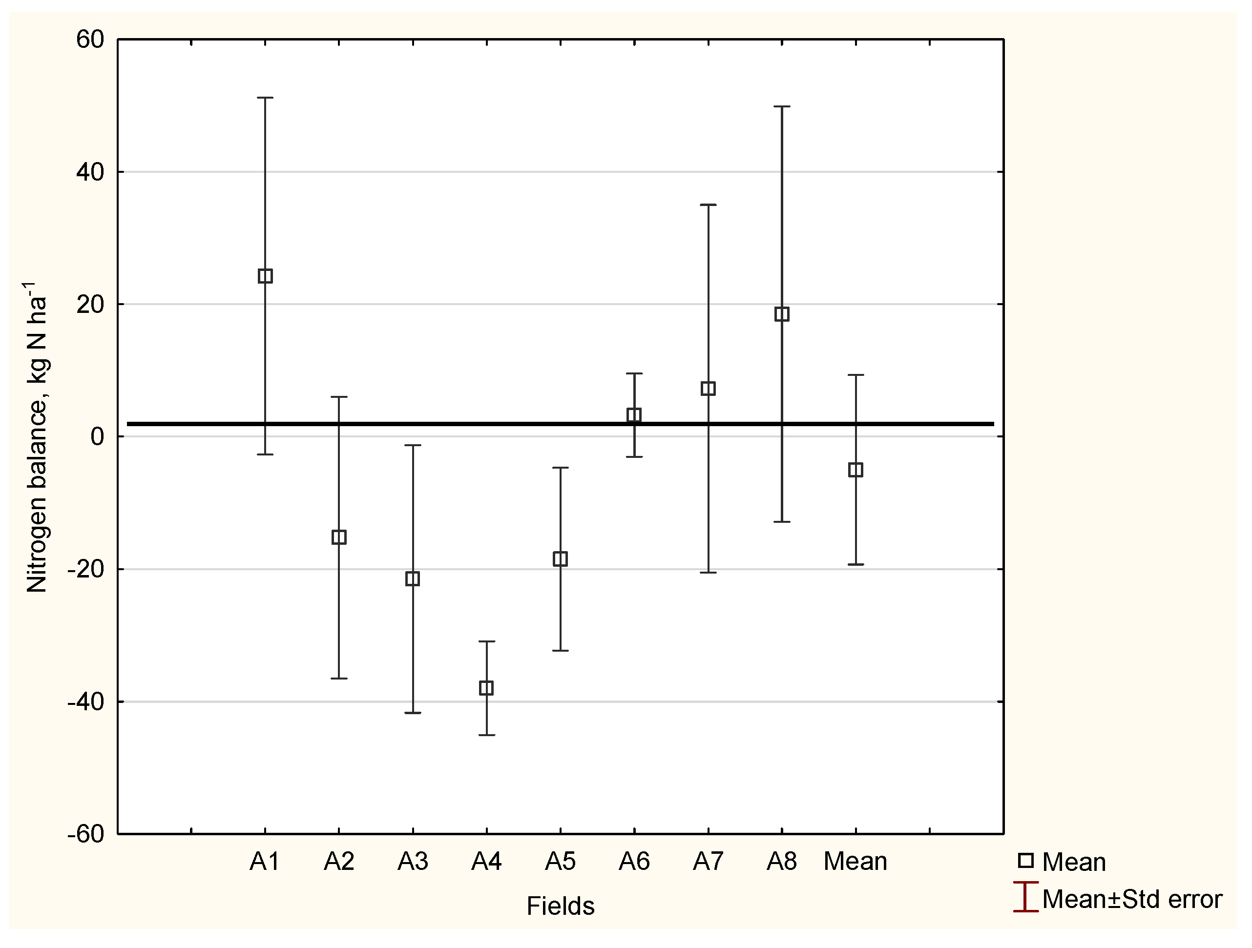
Field Characteristics	Field Number → Decreasing Nitrogen Gap
	4	13	3	11
Nitrogen gap, kg N ha−1	−61	−46	−20	+6
Yield Gap, kg ha−1	−3414	−2614	−1114	+343
Soil usability class	Low	Medium/low	Medium	Medium
Fore-crop	Low	Low	Low	Low
Variety	Medium intensive	Medium intensive	Medium intensive	Intensive
Sowing term	Adequate	Adequate	Adequate	Adequate
Manure	Lack	Lack	Lack	Lack
Soil reaction (pH)	Acidic	Slightly acid	Neutral	Neutral
Phosphorus content—class	Low	Medium	Very high	High
Potassium content—class	Medium	Low	Medium	Medium
Magnesium content class	Low	Medium	High	High
Fungicide protection	Medium	Medium	Medium	Medium

Legend: Low, Medium, High, Adequate—a relative range of the growth factor; Acidic, Slightly acid, Neutral—ranges of soil pH.

, 10 soil and agronomic traits were used to identify the key factors responsible for NG development. The range scale for any production trait should be constructed in a very simple manner, for example, low, medium, high, and in special cases, underlined by “very”. As shown in Figure 8, a NG of 60 kg N ha⁻¹ resulted in a yield gap of 3368 t ha⁻¹. This value is equal to 41.2% of Y_attmax and constitutes 64.8% of the actual harvested yield. The key reasons for the NG development were poor soil quality, inadequate soil pH (acid), and low P content in the soil. The increase in the yield beyond Y_attmax was related to the cultivation of the wheat variety, which responded positively to the optimal soil pH, and an adequate content of the main nutrients.

5. Conclusions

The key assumption of sustainable agriculture production is the effective use of non-renewable means of production available on the farm. First and foremost is the question of total N requirement (by the farm) and its sources. The productivity of each N source (i.e., its efficiency) depends on the farmer’s ability to manage it. The realization of these seemingly contradictory goals depends on the farmer’s knowledge of the N cycles between their farm units, regardless of the farm type. This knowledge must include both the farm’s primary N input (atmospheric N₂ fixation by legumes) and the N recycling processes through livestock manure. On the other hand, it is essential to recognize the N requirements of the cultivated crops, especially during the critical stages of yield formation. These two datasets should form the basis for the purchase of N fertilizer. The simplest diagnostic tool for the farmer is the N balance, which accounts for the N inputs and outputs in the soil/crop system in individual fields on the farm. This method allows for the diagnosis of points (N hotspots) in the N flow that create nutrient losses and lead to production problems and environmental pollution. The nitrogen gap approach forms the basis of determining the maximum attainable yields of crops grown on the farm, or between neighboring farms. To define the NG, only two datasets are needed (i.e., crop yield and the amount of N_f applied). These two management traits permit the maximum yield of a given crop (i.e., the potential N productivity under certain soil conditions) to be established. The NG value for a given field determines its distance from the achievable goal (i.e., high yield under effective N management). The information collected by the farmer on the NG occurrence is crucial in developing an effective program to correct N management on the farm.

References

- Le Mouël, C.; Forslund, A. How can we feed the world in 2050? A review of the responses from global scenario studies. Eur. Rev. Agric. Econ. 2017, 44, 541–591. [Google Scholar] [CrossRef]
- Van Dijk, M.; Morley, T.; Rau, M.L.; Saghai, Y. A meta-analysis of projected global food demand and population at risk of hunger for the period 2010–2050. Nat. Food 2021, 2, 494–501. [Google Scholar] [CrossRef]
- Hunter, M.C.; Smith, R.G.; Schipanski, M.E.; Atwood, L.W.; Mortensen, D.A. Agriculture in 2050: Recalibrating targets for sustainable intensification. BioScience 2017, 67, 386–391. [Google Scholar] [CrossRef] [Green Version]
- Beltran-Peña, A.; Rosa, L.; D’Odorico, P. Global food self-sufficiency in the 21st century under sustainable intensification of agriculture. Environ. Res. Lett. 2020, 15, 095004. [Google Scholar] [CrossRef]
- Keating, B.A.; Herrero, M.; Carberry, P.S.; Gardner, J.; Cole, N.B. Food wedges: Framing the global food demand and supply challenge towards 2050. Glob. Food Sec. 2014, 3, 125–132. [Google Scholar] [CrossRef]
- Röös, E.; Bajželj, B.; Smith, P.; Patel, M.; Little, D.; Garnett, T. Greedey or needy? Land use and climate impacts of food in 2050 under different livestock futures. Glob. Environ. Chang. 2017, 47, 1–12. [Google Scholar] [CrossRef]
- Alexander, P.; Brown, C.; Ameth, A.; Finnigan, J. Human appropriation for land and food: The role of diet. Glob. Environ. Chang. 2016, 41, 88–98. [Google Scholar] [CrossRef] [Green Version]
- Berners-Lee, M.; Kennelly, C.; Watson, R.; Hewitt, C.N. Current global food production is sufficient to meet human nutritional needs in 2050 provided there is radical societal adaptation. Elem. Sci. Anth. 2018, 5, 52. [Google Scholar] [CrossRef]
- Kummu, M.; Fader, M.; Gerten, D.; Guillaume, J.H.A.; Jalava, M.; Jägermeyr, J.; Pfister, S.; Porkka, M.; Siebert, S.; Varis, O. Bringing it al together: Linking measures to secure nations’ food supply. Curr. Opin. Environ. Sustain. 2017, 29, 98–117. [Google Scholar] [CrossRef] [Green Version]
- Harvey, M.; Pilgrim, S. The new competition for land: Food, Energy, and climate change. Food Policy 2011, 36, S40–S50. [Google Scholar] [CrossRef]
- Smith, P.; Gregory, P.J.; van Vuuren, D.; Obersteiner, M.; Havlik, P.; Rounsevell, M.; Woods, J.; Stehfest, E.; Bellarby, J. Competition for land. Phil. Trans. R. Soc. B 2010, 365, 2941–2957. [Google Scholar] [CrossRef] [PubMed] [Green Version]
- Gomiero, T. Soil degradation, land scarcity and food security: Reviewing a complex challenge. Sustainability 2016, 8, 281. [Google Scholar] [CrossRef] [Green Version]
- Kopittke, P.M.; Menzies, N.W.; Wang, P.; McKenza, B.A.; Lombi, E. Soil and the intensification of agriculture for global food security. Environ. Inter. 2019, 132, 105078. [Google Scholar] [CrossRef] [PubMed]
- Taiz, L. Agriculture, plant physiology, and human population growth: Past, present, and future. Theor. Exp. Plant Physiol. 2013, 25, 167–181. [Google Scholar] [CrossRef] [Green Version]
- Erisman, J.W.; Leach, A.; Bleeker, A.; Atwell, B.; Cattaneo, L.; Galloway, J. An integrated approach to a nitrogen use efficiency (NUE) indicator for the food production-consumption chain. Sustainability 2018, 10, 925. [Google Scholar] [CrossRef] [Green Version]
- Ray, D.K.; Mueller, N.D.; West, P.C.; Foley, J.A. Yield trends are insufficient to double global crop production by 2050. PLoS ONE 2013, 8, e66428. [Google Scholar] [CrossRef] [PubMed] [Green Version]
- Conijn, J.G.; Bindraban, P.S.; Schröder, J.J.; Jongschaap, R.E.E. Can our global food system meet food demand within planetary boundries? Agric. Ecosyst. Environ. 2018, 251, 244–256. [Google Scholar] [CrossRef]
- Pradhan, P.; Fischer, G.; van Velthuizen, H.; Reusser, D.E.; Kropp, J.P. Closing yield gaps: How sustainable can we be? PLoS ONE 2015, 10, e0129487. [Google Scholar] [CrossRef] [Green Version]
- The Royal Society. Reaping the Benefits: Science and the Sustainable Intensification of Global Agriculture; RS Policy Document; The Royal Society: London, UK, 2009; p. 86. [Google Scholar]
- Grafton, R.Q.; Williams, J.; Jiang, Q. Food and water gaps to 2050: Preliminary results from the global food and water systems (GFWS) platform. Food Secur. 2015, 7, 209–220. [Google Scholar] [CrossRef] [Green Version]
- Larson, J.A.; Stefanini, M.; Yin, X.; Boyer, C.N.; Lambert, D.M.; Zhou, X.V.; Tubaña, B.S.; Scharf, P.; Varco, J.J.; Dunn, D.J.; et al. Effects of landscape, soils, and weather on yields, nitrogen use, and profitability with sensor-based variable rate nitrogen management in cotton. Agronomy 2020, 10, 1858. [Google Scholar] [CrossRef]
- Grzebisz, W.; Łukowiak, R. Nitrogen gap amelioration is a core for sustainable intensification of agriculture—A concept. Agronomy 2021, 11, 419. [Google Scholar] [CrossRef]
- Bodirsky, B.L.; Popp, A.; Lotze-Campen, H.; Dietrich, J.P.; Rolinski, S.; Weindl, I.; Smitz, C.; Müller, C.; Bonsch, M.; Humpenöder, F.; et al. Reactive nitrogen requirements to feed the world in 2050 and potential to mitigate nitrogen pollution. Nat. Commun. 2014, 5, 3858. [Google Scholar] [CrossRef] [PubMed] [Green Version]
- Lassaletta, L.; Billen, G.; Garnier, J.; Bouwman, L.; Velazquez, E.; Muleller, N.D.; Gerber, J.S. Nitrogen use in the global system: Past trends and future trajectories of agronomic performance, pollution, trade, and dietary demand. Environ. Res. Lett. 2016, 11, 095007. [Google Scholar] [CrossRef]
- Haene, K.D.; Salomez, J.; De Neve, S.; De Waele, J.; Hofman, G. Environmental performance of nitrogen fertilizer limits imposed by the EU Nitartes Directive. Agric. Ecosyst. Environ. 2014, 192, 67–79. [Google Scholar] [CrossRef]
- Oenema, O.; Pietrzak, S. Nutrient management in food production. Achieving agronomic and environmental targets. Ambio 2003, 31, 159–168. [Google Scholar] [CrossRef] [PubMed]
- Lemaire, G.; Jeuffroy, M.-H.; Gastal, F. Diagnosis tool for plant an crop N status in vegetative stage: Theory and practices for crop N management. Eur. J. Agron. 2008, 28, 181–190. [Google Scholar] [CrossRef]
- Córdova, C.; Barrera, J.A.; Magna, C. Spatial variation in nitrogen mineralization as a guide for variable application of nitrogen fertilizer to cereal crops. Nutr. Cycl. Agroecosyst. 2018, 110, 83–88. [Google Scholar] [CrossRef]
- Schilizzi, S.; Pannel, D.J. The economics of nitrogen fixation. Agronomie 2001, 21, 527–537. [Google Scholar] [CrossRef] [Green Version]
- Gutser, R.; Ebertseder, T.; Weber, A.; Schraml, M.; Schmidhalter, U. Short-term and residual availability of nitrogen after long-term application of organic fertilizers on arable land. J. Plant Nutr. Soil. Sci. 2005, 168, 439–446. [Google Scholar] [CrossRef]
- Bussink, D.W.; Oenema, O. Ammonia volatilization from dairy farming systems in temperate areas. A review. Nutr. Cycl. Agroecosyst. 1998, 51, 19–33. [Google Scholar] [CrossRef]
- Mary, B.; Recous, S.; Darwis, D.; Robin, D. Interactions between decomposition of plant residues and nitrogen cycling in soil. Plant Soil 1996, 181, 71–82. [Google Scholar] [CrossRef]
- Smil, V. Nitrogen in crop production: An account of global flows. Glob. Biogeochem. Cycles 1999, 13920, 647–662. [Google Scholar] [CrossRef] [Green Version]
- de Vries, W.; Schulte-Uebbing, L.; Kros, H.; Voogd, J.C.; Louwagie, G. Spatially explicit boundaries for agricultural nitrogen inputs in the European Union to meet air and water quality target. Sci. Total Environ. 2021, 786, 147283. [Google Scholar] [CrossRef] [PubMed]
- Luce, M.S.; Whalen, J.K.; Ziadi, N.; Zebarth, B.J. Nitrogen dynamics and indices to predict soil nitrogen supply in humid temperate soils. Adv. Agron. 2011, 112, 55–102. [Google Scholar]
- Grzebisz, W.; Łukowiak, R.; Sassenrath, G. Virtual nitrogen as a tool for assessment of nitrogen at the field scale. Field Crops Res. 2018, 218, 182–184. [Google Scholar] [CrossRef]
- Olfs, H.-W.; Blankenau, K.; Brentrup, F.; Jasper, J.; Link, A.; Lammel, J. Soil- and plant-based nitrogen-fertilizer recommendations in arable farming. J. Plant Nutr. Soil Sci. 2005, 168, 414–431. [Google Scholar] [CrossRef]
- Barłóg, P.; Łukowiak, R.; Grzebisz, W. Predicting the content of soil mineral nitrogen based on the content of calcium chloride-extractable nutrients. J. Plant Nutr. Soil Sci. 2017, 180, 624–635. [Google Scholar] [CrossRef]
- Dobermann, A. Nitrogen use efficiency—State of the art. In Proceedings of the IFA International Workshop on Enhanced Efficiency Fertilizers, Frankfurt, Germany, 28–30 June 2005; pp. 1–16. [Google Scholar]
- Liu, Y.; Wu, L.; Baddeley, J.A.; Watson, C.A. Models of biological nitrogen fixation of legumes. Sustain. Agric. 2011, 2, 883–905. [Google Scholar]
- Schimel, J.P.; Bennett, J. Nitrogen mineralization: Challenges of a changing paradigm. Ecology 2004, 85, 591–602. [Google Scholar] [CrossRef]
- Marschner, H. Mineral Nutrition of Higher Plants; Academic Press: London, UK, 1995; 899p. [Google Scholar]
- Masson-Boivin, C.; Sachs, J.L. Symbiotic nitrogen fixation by rhizobia—The roots of a success story. Curr. Opin. Plant Biol. 2018, 44, 7–15. [Google Scholar] [CrossRef] [Green Version]
- Soumare, A.; Giedhiou, A.; Thuita, M.; Hafidi, M.; Ouhdouch, Y.; Gopalakrishnan, S.; Kousni, L. Exploiting biological nitrogen fixation: A route towards sustainable agriculture. Plants 2020, 9, 1011. [Google Scholar] [CrossRef] [PubMed]
- Masson-Boivin, C.; Giraud, E.; Perret, X.; Batut, J. Establishing nitrogen-fixing symbiosis with legumes: How many rhizobium recipes? Trends Microbiol. 2009, 17, 458–466. [Google Scholar] [CrossRef] [PubMed]
- Davies-Barnard, T.; Friedlingstein, P. The Global Distribution of Biological Nitrogen Fixation in Terrestrial Natural Ecosystems. Glob. Biogeochem. Cycles 2020, 34, e2019GB006387. [Google Scholar] [CrossRef]
- Bever, J.D.; Simms, E.L. Evolution of nitrogen fixation in spatially structured populations of Rhizobium. Heredity 2000, 85, 366–372. [Google Scholar] [CrossRef]
- McFall-Ngai, M.J.; Gordon, J.I. Experimental Models of Symbiotic Host-Microbial Relationships: Understanding the Underpinnings of Beneficence and the Origins of Pathogenesis. In Evolution of Microbial Pathogens; Steven, H., DiRita, V.J., Eds.; Jon Wiley & Sons Inc.: New York, NY, USA, 2006; Volume 9, pp. 147–166. [Google Scholar]
- Voisin, A.S.; Salon, C.; Jeudy, C.; Warembourg, F.R. Symbiotic N2 fixation activity in relation to C economy of Pisum sativum L. as a function of plant phenology. J. Exp. Bot. 2003, 54, 2733–2744. [Google Scholar] [CrossRef] [Green Version]
- Kahindi, J.H.; Karanja, N.K. Essentials of Nitrogen Fixation Biotechnology. Biotechnol.-Vol. VIII Fundam. Biotechnol. 2009, 8, 54–80. [Google Scholar]
- Sujkowska, M. The course of the infection process in the symbiotic system of legumes-Rhizobium. Bot. News 2009, 53, 35–53. [Google Scholar]
- Martyniuk, S. Production of microbial preparations: Symbiotic bacteria of legumes as an ex ample. J. Res. Appl. Agric. Eng. 2010, 55, 20–23. [Google Scholar]
- Nannipieri, P.; Ascher, J.; Ceccherini, M.T.; Landi, L.; Pietramellara, G.; Renella, G.; Valori, F. Microbial diversity and microbial activity in the rhizosphere. Cienc. Del Suelo 2007, 25, 89–97. [Google Scholar]
- Pathak, J.; Rajneesh; Maurya, P.K.; Singh, S.P.; Häder, D.-P.; Sinha, R.P. Cyanobacterial farming for environment friendly sustainable agriculture practices: Innovations and perspectives. Front. Environ. Sci. 2018, 6, 7. [Google Scholar] [CrossRef]
- Waraczewska, Z.; Niewiadomska, A. Diazotroph—Characteristics of the symbiotic legume—Rhizobium. In Leguminous Plants in Polish Agriculture: Genetics, Breeding, Cultivating and Using; Poznan University of Life Science: Poznań, Poland, 2017; pp. 83–94. [Google Scholar]
- Zahran, H.H. Rhizobia from wild legumes: Diversity, taxonomy, ecology, nitrogen fixation and biotechnology. J. Biotech. 2001, 91, 143–153. [Google Scholar] [CrossRef]
- Graham, P.H. Stress tolerance in Rhizobium and Bradyrhizobium, and nodulation under adverse soil conditions. Can. J. Microbiol. 1992, 38, 475–484. [Google Scholar] [CrossRef]
- Aranjuelo, I.; Aldasoro, J.; Arrese-Igor, C.; Erice, G.; Sanz-Sáez, Á. How Does High Temperature Affect Legume Nodule Symbiotic Activity? In Legume Nitrogen Fixation in a Changing Environment; Sulieman, S., Tran, L.S., Eds.; Springer: Cham, Switzerland, 2015. [Google Scholar]
- Fageria, N.K.; Nascente, A.S. Management of soil acidity of South American soils for sustainable crop production. Adv. Agron. 2014, 128, 221–275. [Google Scholar]
- Martinze-Hidalgo, P.; Hirsch, A.M. The nodule microbiome: N2-fixing Rhizobia do not live alone. Phytobiomes 2017, 1, 70–82. [Google Scholar] [CrossRef] [Green Version]
- Kochian, L.V.; Hoekenga, O.A.; Piñeros, M.A. How do crop plants tolerate acid soils? Mechanism of aluminum tolerance and phosphorus efficiency. Annu. Rev. Plant Biol. 2004, 55, 459–493. [Google Scholar] [CrossRef]
- Niewiadomska, A.; Sulewska, H.; Wolna-Maruwka, A.; Ratajczak, K.; Waraczewska, Z.; Budka, A. The Influence of Bio-Stimulants and Foliar Fertilizers on Yield, Plant Features, and the Level of Soil Biochemical Activity in White Lupine (Lupinus albus L.) Cultivation. Agronomy 2020, 10, 150. [Google Scholar] [CrossRef] [Green Version]
- Weisany, W.; Raei, Y.; Allahverdipoor, K.H. Role of some of mineral nutrients in biological nitrogen fixation. Bulletin of Environment. Pharmacol. Life Sci. 2013, 2, 77–84. [Google Scholar]
- Sadeghipour, O.; Abbasi, S. Soybean response to drought and seed inoculation. World Appl. Sci. J. 2012, 17, 55–60. [Google Scholar]
- Cooper, J.; Scherer, H. Nitrogen Fixation. In Mineral Nutrition of Higher Plants, 3rd ed.; Marchner, P., Ed.; Academic Press: London, UK, 2012; pp. 389–408. [Google Scholar]
- Roy, R.N.; Finck, A.; Blair, G.J.; Tandon, H.L.S. Plant nutrition for food security. A guide for integrated nutrient management. FAO Fertil. Plant Nutr. Bull. 2006, 16, 368. [Google Scholar]
- Bambara, S.; Ndakidemi, P.A. The potential roles of lime and molybdenum on the growth, nitrogen fixation and assimilation of metabolites in nodulated legumes: A special reference to Phaseolus vulgaris L. African J. Biotech. 2010, 8, 2482–2489. [Google Scholar]
- Bellaloui, N.; Mengistu, A.; Kasses, M.A.; Abel, C.A.; Zobiole, L.H.S. Role of boron nutrient in nodules growth and nitrogen fixation in soybean genotypes under water stress conditions. In Advance in Biology and Ecology of Nitrogen Fixation; Ohyama, T., Ed.; InTech: London, UK, 2014; pp. 237–258. [Google Scholar]
- Hu, X.; Wei, X.; Ling, J.; Chen, J. Cobalt: An essential micronutrient for plant growth. Front. Plant Sci. 2021, 16, 768523. [Google Scholar] [CrossRef]
- Stagnari, F.; Maggio, A.; Galieni, A.; Pisante, M. Multiple benefits of legumes for agriculture sustainability. Chem. Biol. Technol. Agric. 2017, 4, 2. [Google Scholar] [CrossRef] [Green Version]
- Torma, S.; Vilček, J.; Lošák, T.; Kužel, S.; Martensson, A. Residual plant nutrients in crop residues—An importnat resource. Acta Agric. Scand. Sec. B Soil Plant Sci. 2017, 68, 358–366. [Google Scholar]
- Kumar, T.K.; Rana, D.S.; Nain, L. Legume residue and N management for improving productivity and N economy and soil fertility in wheat (Triticum aestivum)—Based cropping system. Natl. Acad. Sci. Lett. 2019, 42, 297–307. [Google Scholar] [CrossRef]
- Ludwig, B.; Geisseler, D.; Michel, K.; Joergensen, R.G.; Schulz, E.; Merbach, I.; Raupp, J.; Rauner, R.; Hu, K.; Niu, L.; et al. Effects of fertilization and soil management on crop yields and carbon stabilization in soils. A review. Agron. Sustain. Dev. 2011, 31, 361–372. [Google Scholar] [CrossRef] [Green Version]
- Bauer, A.; Black, A.L. Quantification of the effect of soil organic matter content on soil productivity. Soil Sci. Soc. Am. J. 1994, 58, 185–193. [Google Scholar] [CrossRef]
- Karlen, D.L.; Lal, R.; Follet, R.F.; Komble, J.M.; Hatfield, R.D.; Miranowski, J.M.; Cambardella, C.A.; Manale, A.; Anex, R.P.; Rice, C.W. Crop residues: The rest of the story. Environ. Sci. Technol. 2009, 43, 8011–8015. [Google Scholar] [CrossRef] [Green Version]
- Scotti, R.; Bonanomii, G.; Scelza, R.; Zoina, A.; Rao, M.A. Organic amendments as sustainable tool to recovery soil fertility in intensive agricultural systems. J. Soil Sci. Plant Nutr. 2015, 15, 333–352. [Google Scholar]
- Parton, W.; Schimel, D.; Cole, C.; Ojima, D. Analysis of factors controlling soil organic matter in great plains grasslands. Soil. Sci. Soc. Am. 1987, 51, 1173–1179. [Google Scholar] [CrossRef]
- Stevenson, F.J. Cycles of Soil; John Wiley & Sons: New York, NY, USA, 1986; 380p. [Google Scholar]
- Bolinder, M.A.; Crotty, F.; Elsen, A.; Feąc, M.; Kismányoky, T.; Lipiec, J.; Tits, M.; Tóth, Z.; Kätterer, T. The effect of crop residues, cover crops, manures and nitrogen fertilziation on soil organic carbon changes in agroecosystems: A synthesis of reviews. Mitig. Adapt. Strateg. Glob. Chang. 2020, 25, 929–952. [Google Scholar] [CrossRef]
- Koishi, A.; Bragazza, L.; Maltas, A.; Guillaume, T.; Sinaj, S. Lon-term efefcts of organic amendments on soil organic matetr quantity and quality in conventional cropping systems in Switzerland. Agronomy 2020, 10, 1977. [Google Scholar] [CrossRef]
- Hiel, M.P.; Chélin, M.; Prvin, N.; Barbieux, S.; Degrune, F.; Lemtiri, A.; Colinet, G.; Degré, A.; Bodson, B.; Garré, S. Crop residue management in arable cropping systems under temperate climate. Part 2. Soil physical properties and crop production. A review. Biotechnol. Agron. Sci. Environ. 2016, 20, 2450256. [Google Scholar] [CrossRef]
- Wnuk, A.; Górny, A.G.; Bocianowski, J.; Kozak, M. Visualizing harvest index in crops. Comm. Biometry Crop Sci. 2013, 8, 48–59. [Google Scholar]
- Stepaniuk, M.; Głowacka, A. Yield of winter oilseed rape (Brassica napus L. var. bnapus) in a short-term monoculture and the macronutrient accumulation in relation to the dose and method of Sulphur application. Agronomy 2022, 12, 68. [Google Scholar] [CrossRef]
- Grzebisz, W. Crop Plants Fertilization. Part 2. Fertilizers and Fertilization Systems; PWRiL: Poznań, Poland, 2015; 396p. (In Polish) [Google Scholar]
- Zhao, X.; Yuan, G.; Wang, H.; Lu, D.; Chen, X.; Zhou, J. Effects of full straw incorporation on soil fertility and crop yield in rice-wheat rotation for silty clay loamy cropland. Agronomy 2019, 9, 133. [Google Scholar] [CrossRef] [Green Version]
- Venkatramanan, V.; Shah, S.; Rai, A.K.; Prasad, R. Nexus between Crop Residue Burning, Bioeconomy and Sustainable Development Goals Over North-Western India. Front. Energy Res. 2021, 392. [Google Scholar] [CrossRef]
- Kamusoko, R.; Jingura, R.M.; Parawira, W.; Chikwambi, Z. Strategies for valorization of crop residues into biofuels and other value-added products. Biofpr 2021, 15, 1950–1964. [Google Scholar] [CrossRef]
- Sarkar, S.; Skalicky, M.; Hossain, A.; Brestic, M.; Saha, S.; Gorai, S.; Ray, K.; Brahmachari, K. Management of crop residues for improving input use efficiency and agricultural sustainability. Sustainability 2020, 12, 9808. [Google Scholar] [CrossRef]
- Parmar, A.; Sturm, B.; Hensel, O. Crops that feed the world: Production and improvement of cassava for food, feed and industrial uses. Food Secur. 2017, 9, 907–927. [Google Scholar] [CrossRef]
- Whitemore, A.P.; Groot, J.J.R. The decomposition of sugar beet residues: Mineralization versus immobilization in contrasting soil types. Plant Soil 1997, 192, 237–247. [Google Scholar] [CrossRef]
- Tomaszewska, J.; Bieliński, D.; Binczarski, M.; Berlowska, J.; Dziugan, P.; Piotrowski, J.; Stanishevsky, A.; Witońska, I.A. Products of sugar beet processing as raw materials for chemical and biodegradable polymers. RSC Adv. 2018, 8, 3161. [Google Scholar] [CrossRef] [PubMed] [Green Version]
- Rotz, C.A. Management to reduce nnitrogen losses in animal production. J. Anim. Sci. 2004, 82, E119–E137. [Google Scholar] [PubMed]
- Loyon, L. Overview of animal manure management for beef, pig, and poultry in France. Front. Sustain. Food Syst. 2018, 2, 36. [Google Scholar] [CrossRef]
- Sefeedpari, P.; Pudełko, R.; Jędrejek, A.; Kozak, M.; Borzęcka, M. To what extent is manure produced, distributed and potentially available for bioenergy? A step toward stimulating circular bio-economy in Poland. Energies 2020, 13, 6266. [Google Scholar] [CrossRef]
- ASAE. Manure Production and Characteristics; American Society of Agricultural and Biological Engineers: St. Joseph, MI, USA, 2014; Volume D384.1 DEC99 (R2014). [Google Scholar]
- Misselbrook, T.H.; Powell, J.M. Influence of bedding material on ammonia emissions from cattle excreta. J. Dairy Sci. 2005, 88, 4304–4312. [Google Scholar] [CrossRef]
- Kupper, T.; Hani, C.; Neftel, A.; Kincaid, C.; Buhler, M.; Amon, B.; Vander Zaag, A. Ammonia and greenhouse gas emissionsw from slurry storage—A review. Agric. Ecosyst. Environ. 2020, 300, 106963. [Google Scholar] [CrossRef]
- Whitehead, D.C.; Raistrick, N. Nitrogen in excreta if dairy cattle: Changes during short-term storage. J. Agric. Sci. 1993, 21, 73–81. [Google Scholar] [CrossRef]
- Paul, J.W.; Beauchamp, E.G. Nitrogen availability for corn in soils amended with urea, cattle slurry, and solid and composted manure. Can. J. Soil Sci. 1993, 73, 253–266. [Google Scholar] [CrossRef]
- Fangueiro, D.; Hjorth, M.; Gioelli, F. Acidification of animal slurry—A review. J. Environ. Manag. 2015, 149, 46–56. [Google Scholar] [CrossRef]
- Christensen, M.; Sommer, S. Manure characterization and inorganic chemistry. In Animal Manure Recycling: Treatment and Management; Sommer, S., Christensen, M., Schmidt, T., Jensen, L., Eds.; John Wiley & Sons. Ltd.: Chichester, UK, 2013. [Google Scholar]
- Boratyński, K. Organic Fertilizers; PWRiL: Warsaw, Poland, 1977; 231p. (In Polish) [Google Scholar]
- Dou, Z.; Koln, R.; Ferguson, J.; Boston, R.; Newbold, J. Managing nitrogen on dairy farms. An integrated approach. I. Model description. J. Dairy Sci. 1996, 79, 2071–2080. [Google Scholar] [CrossRef]
- Chen, B.; Liu, E.; Tian, Q.; Yan, C.; Zhang, Y. Soil nitrogen dynamics and crop residues. A review. Agron. Sustain. Dev. 2014, 34, 429–442. [Google Scholar] [CrossRef] [Green Version]
- Grzyb, A.; Wolna-Maruwka, A.; Niewiadomska, A. Environmental factors affecting the mineralization of crop residues. Agronomy 2020, 10, 1951. [Google Scholar] [CrossRef]
- Hijbeek, R.; Ten Berge, H.F.; Whitemore, A.P.; Barkusky, D.; Schroder, J.J.; van Ittersum, M.K. Nitrogen fertiliser replacement values for organic amendments appear to increase with N application rates. Nutr. Cycl. Agroecosyst. 2018, 110, 105–118. [Google Scholar] [CrossRef] [Green Version]
- Kumar, P.; Tarafdar, J.C.; Panwar, J.; Kathju, S. A rapid method for assessment of plant residue quality. J. Plant Nutr. Soil Sci. 2003, 166, 662–666. [Google Scholar] [CrossRef]
- Rahn, C.R.; Bending, G.D.; Turner, M.K.; Lillywhite, R.D. Management of N mineralization from crop residues of high N content using amendment materials of varying quality. Soil Use Manag. 2003, 19, 193–200. [Google Scholar] [CrossRef]
- Obalum, S.E.; Chibuike, G.U.; Peth, S.; Ouyang, Y. Soil organic matter as sole indicator of soil degradation. Environ. Monit. Assess. 2017, 189, 176. [Google Scholar] [CrossRef]
- Spychalski, W.; Grzebisz, W.; Diatta, J.; Kostarev, D. Humus stock degradation and impacts on phosphorus forms in arable soils—A case of the Ukrainian Forest Steppe Zone. Chem. Spec. Bioavail. 2018, 30, 33–46. [Google Scholar] [CrossRef] [Green Version]
- Wadman, W.P. Effect of organic manure on crop yield in long-term field experiments. INTECOL Bull. 1987, 15, 83–89. [Google Scholar]
- Gross, A.; Glase, B. Meta-analysis on how manure application changes soil organic carbon storage. Sci. Rep. 2022, 11, 5516. [Google Scholar] [CrossRef]
- Przygocka-Cyna, K.; Grzebisz, W. The multifactorial effect of digestate on the availability of soil elements and grain yield and its mineral profile. Agronomy 2020, 10, 275. [Google Scholar] [CrossRef] [Green Version]
- Ötvös, K.; Marconi, M.; Vega, A.; O’brian, J.; Johnston, A.; Abualla, R.; Antonielli, L.; Montesinos, J.C.; Zhang, Y.; Yan, S.; et al. Modulation of plant root growth by nitrogen source-defined regulation of polar auxin transport. EMBO J. 2021, 40, e106862. [Google Scholar] [CrossRef] [PubMed]
- Spiertz, J.H.J. Nitrogen, sustainable agriculture and food security. A review. Agron. Sustain. Dev. 2010, 30, 43–55. [Google Scholar] [CrossRef] [Green Version]
- Tegeder, M.; Masclaux-Daubresse, C. Source and sink mechanism of nitrogen transport and use. New Phytol. 2018, 217, 35–53. [Google Scholar] [CrossRef] [PubMed] [Green Version]
- Sondergaard, T.E.; Schulz, A.; Palmgreen, M.G. Energization of transport processes in plants. Roles of the plasma membrane H+-ATPase. Plant Physiol. 2004, 136, 2475–2482. [Google Scholar] [CrossRef] [Green Version]
- Masoni, A.; Ercoli, L.; Mariotti, M.; Arduini, I. Post–anthesis accumulation and remobilization of dry matter, nitrogen and phosphorus in durum wheat as affected by soil type. Eur. J. Agron. 2007, 26, 179–186. [Google Scholar] [CrossRef]
- Luo, L.; Zhang, Y.; Xu, G. How does nitrogen shape plant architecture. J. Exp. Bot. 2020, 71, 4415–4427. [Google Scholar] [CrossRef]
- Hu, Q.-Q.; Shu, J.-Q.; Lin, W.-M.; Zhang, G.-Z. Role of auxin and nitrate signaling in the development of root system architecture. Front. Plant Sci. 2021, 12, 690363. [Google Scholar] [CrossRef]
- Lynch, J.L. Steep, cheap and deep: An ideotype to optimize water and N acquisition by maize root systems. Ann. Bot. 2013, 112, 347–357. [Google Scholar] [CrossRef] [Green Version]
- Falhof, J.; Pedersen, J.T.; Fuglsang, A.T.; Palmgren, M. Plasma Membrane H+ -ATPase Regulation in the Center of Plant Physiology. Mol. Plant. 2016, 9, 323–337. [Google Scholar] [CrossRef] [Green Version]
- Muratore, C.; Espen, L.; Prinsi, B. Nitrogen uptake in plants: The plasma membrane root transport systems from a physiological proteomic perpective. Plants 2021, 10, 681. [Google Scholar] [CrossRef]
- Marschner, H.; Kirkby, E.A.; Cakmak, J. Effect of mineral nutrition on shoot-root partitioning of photo-assimilates and cycling of mineral nutrients. J. Exp. Bot. 1996, 47, 1255–1263. [Google Scholar] [CrossRef] [PubMed]
- McGuire, A.M.; Bryant, D.C.; Denison, R.F. Wheat yields, nitrogen uptake, and soil moisture following winter legume cover crop vs. Fallow. Agron. J. 1998, 90, 404–410. [Google Scholar] [CrossRef] [Green Version]
- Barłog, P.; Grzebisz, W. Effect of timing and nitrogen fertilizer application on winter oilseed rape (Brassica napus L.). II. Nitrogen uptake dynamics and fertilizer efficiency. J. Agron. Crop Sci. 2004, 190, 314–323. [Google Scholar] [CrossRef]
- Barraclough, P.B. The growth and activity of winter wheat roots in the field: Nutrient uptakes of high-yielding crops. J. Agric. Sci. Camb. 1986, 106, 45–52. [Google Scholar] [CrossRef]
- Grzebisz, W.; Szczepaniak, W.; Grześ, S. Sources of nutrients for high-yielding winter oilseed rape (Brassica napus L.) during post-flowering growth. Agronomy 2020, 10, 626. [Google Scholar] [CrossRef]
- Sylvester-Bradley, R.; Lunn, G.; Foulkes, J.; Shearman, V.; Spink, J.; Ingram, J.; Management Strategies for Yield of Cereals and Oilseed Rape. HGCA Conference: Agronomic Intelligence: The Basis for Profitable Production. HGCA. (Vol. 18). Available online: www.hgca.com/publications (accessed on 14 November 2021).
- Gruber, B.D.; Giehl, R.F.H.; Friedel, S.; von Wiren, N. Plasticity of the Arabidopsis root system under nutrient deficiencies. Plant Physiol. 2013, 163, 161–179. [Google Scholar] [CrossRef] [Green Version]
- Mayer, U. BBCH Monograph. In Growth Stages of Mono- and Dicotyledonous Plants, 2nd ed.; Federal Biological Research Center for Agriculture and Forestry: Berlin, Germany, 2001; Available online: http://www.jki.bund.de/fileadmin/dam_uploads/_veroeff/bbch/BBCH-Skala_Englisch.pdf (accessed on 14 March 2021).
- Yin, X.; Goudriaan, J.; Lantinga, E.A.; Vos, J.; Spiertz, H. A flexible sigmoid function of determinate growth. Ann. Bot. 2003, 91, 361–371. [Google Scholar] [CrossRef]
- Kurepa, J.; Smalle, J.A. Auxin/cytokinin antagonistic control of the shoot/root growth ration and its relevance for adaptation to growth and nutrient deficiency stress. Int. J. Mol. Sci. 2022, 23, 1933. [Google Scholar] [CrossRef]
- Koprna, R.; Humplik, J.F.; Spisek, Z.; Bryksova, M.; Zatloukal, M.; Mik, V.; Novak, O.; Nisler, J.; Dolezal, K. Improvement of tillering and grain yield by application of cytokinin derivatives in wheat and barley. Agronomy 2021, 11, 67. [Google Scholar] [CrossRef]
- Slafer, G.A.; Elia, M.; Savin, R.; Garcia, G.A.; Terrile, I.I.; Ferrante, A.; Miralles, D.J.; González, F.G. Fruiting efficiency: An alternative trait to further rise in wheat yield. Food Energy 2015, 4, 92–109. [Google Scholar] [CrossRef]
- Klepper, B.; Rickman, R.W.; Waldman, S.; Chevalier, P. The physiological life cycle of wheat: Its use in breeding and crop management. Euphytica 1998, 100, 341–347. [Google Scholar] [CrossRef]
- Guo, Z.; Chen, D.; Schnurbusch, T. Plant and floret growth at distinct developmental stages during the stem elongation phase in wheat. Front. Plant. Sci. 2018, 9, 330. [Google Scholar] [CrossRef] [PubMed] [Green Version]
- Xie, Q.; Mayes, S.; Sparkes, D.L. Preanthesis biomass accumulation and plant organs defines yield components in wheat. Eur. J. Agron. 2016, 81, 15–26. [Google Scholar] [CrossRef]
- Barłóg, P. Effect of magnesium and nitrogen fertilizers on the growth and alkaloid content of Lupinus angustifolius L. Aust. J. Agric. Res. 2002, 53, 671–676. [Google Scholar] [CrossRef]
- Kong, L.G.; Xie, Y.; Hu, L.; Feng, B.; Li, S.D. Remobilization of vegetative nitrogen to developing grain in wheat (Triticum aestivum L.). Field Crops Res. 2016, 196, 134–144. [Google Scholar] [CrossRef]
- Spiertz, J.; Vos, J. Grain Growth of Wheat and Its Limitation by Carbohydrate and Nitrogen Supply. In Wheat Growth and Modelling; Day, W., Atkin, R., Eds.; Plenum Press: New York, NY, USA, 1985. [Google Scholar]
- Bergmann, W. Nutritional Disorders of Plants; Verlag Gustav Fisher: Jena, Germany, 1992; p. 741. [Google Scholar]
- Elwali, A.; Gasho, G.; Summer, M. DRIS norms for 11 nutrients in con leaves. Agronomy J. 1985, 77, 506–508. [Google Scholar] [CrossRef]
- Matus, F.J.; Rodriguez, J. A simple method for estimating the contribution of nitrogen mineralization to nitrogen supply of crops from a stabilized pool of soil organic matter and recent organic input. Plant Soil 1994, 162, 259–271. [Google Scholar] [CrossRef]
- Iwańska, M.; Paderewski, J.; Stępień, M.; Rodrigues, P.C. Adaptation of winter wheat cultivars to different environments: A case study in Poland. Agronomy 2020, 10, 632. [Google Scholar] [CrossRef]
- Berbell, J.; Martinez-Dalmau, J. A simple agro-economic model for optimal farm nitrogen application under yield uncertainty. Agronomy 2021, 11, 1107. [Google Scholar] [CrossRef]
- Tabak, M.; Lepiarczyk, A.; Filipek–Mazur, B.; Lisowska, A. Efficiency of Nitrogen Fertilization of Winter Wheat Depending on Sulfur Fertilization. Agronomy 2020, 10, 1304. [Google Scholar] [CrossRef]
- Szczepaniak, W.; Nowicki, N.; Bełka, D.; Kazimierowicz, A.; Kulwicki, M.; Grzebisz, W. Effect of foliar application of micronutrients and fungicides on the nitrogen use efficiency in winter wheat. Agronomy 2022, 12, 257. [Google Scholar] [CrossRef]
- MvLellan, E.L.; Cassman, K.G.; Eagle, A.J.; Woodbury, P.B.; Sela, S.; Tonitto, C.; Marjerison, R.D.; van Es, H.M. The nitrogen balancing act: Tracking the environmental performance of food production. Bioscience 2018, 68, 194–203. [Google Scholar] [CrossRef] [PubMed]
- Petersen, R.J.; Blicher-Mathiesen, G.; Rolighed, J.; Andersen, H.E.; Kronvang, B. Three decades of regulation of nitrogen losses: Experiences from the Danish Agricultural Monitoring program. Sci. Total Environ. 2021, 787, 147619. [Google Scholar] [CrossRef] [PubMed]
- Delphin, J.-E. Estimation of nitrogen mineralization in the field from an incubation test and from soil analysis. Agronomie 2000, 20, 349–361. [Google Scholar] [CrossRef] [Green Version]
- Li, S.-X.; Wang, Z.-H.; Miao, Y.-F.; Li, S.-Q. Soil organic nitrogen and its contribution to crop production. J. Integr. Agric. 2014, 139, 2061–2080. [Google Scholar] [CrossRef]
- Parris, K. Agricultural nutrient balances as agri-environmental indicators: An OECD perspective. Environ. Pollut. 1998, 102 (Suppl. S1), 219–225. [Google Scholar] [CrossRef]
- van Beek, C.L.; Brouver, L.; Oenema, O. The use of farmgate balances and soil surface balances an estimator for nitrogen leaching to surface water. Nutr. Cycl. Agroecosyst. 2003, 67, 233–244. [Google Scholar] [CrossRef]
- Oenema, O.; Kros, H.; de Vries, W. Approaches and uncertainties in nutrient budget: Implications for nutrient managment and environmental policies. Eur. J. Agron. 2003, 20, 3–16. [Google Scholar] [CrossRef]
- Blesh, J.; Drinkwater, L.E. The impact of nitrogen source and crop rotation on nitrogen mass balance in the Mississippi River Basin. Ecol. Appl. 2013, 23, 1017–1035. [Google Scholar] [CrossRef]
- Rayne, N.; Aula, L. Livestock manure and its impacts on soil health: A review. Soil Syst. 2020, 4, 64. [Google Scholar] [CrossRef]
- Ren, T.; Wang, J.; Chen, Q.; Zhang, F.; Lu, S. The effects of manure and nitrogen fertilizer applications on soil organic carbon and nitrogen in a high-input cropping system. PLoS ONE 2014, 9, e97732. [Google Scholar] [CrossRef] [PubMed]
- Evans, L.T.; Fischer, R.A. Yield potential: Its definition, measurement, and significance. Crop Sci. Soc. Am. 1999, 39, 1544–1551. [Google Scholar] [CrossRef]
- Licker, R.; Johnston, M.; Foley, J.A.; Barford, C.; Kucharik, C.J.; Monfreda, C.; Ramankutty, N. Mind the gap: How do climate and agricultural management explain the “yield gap” of croplands around the world? Glob. Ecol. Biogeogr. 2010, 19, 769–782. [Google Scholar] [CrossRef]
- Rabbinge, R. The ecological background of food production. In Crop Production and Sustainable Agriculture; Rabbinge, R., Ed.; John Wiley and Sons: New York, NY, USA, 1993; pp. 2–29. [Google Scholar]
- Grzebisz, W.; Diatta, J. Constrains and solutions to maintain soil productivity, a case study from Central Europe. In Soil Fertility Improvement and Integrated Nutrient Management—A Global Perspective; Whalen, J., Ed.; InTech: London, UK, 2012; pp. 159–183. ISBN 978–953–307–945–5. [Google Scholar]