AquaCrop Model Evaluation for Winter Wheat under Different Irrigation Management Strategies: A Case Study on the North China Plain

Abstract

The North China Plain (NCP) produces about half of the winter wheat yield in China; therefore, it is essential to improve winter wheat grain yield, biomass, and water productivity (WP) under current water shortage conditions in this area. In this study, the AquaCrop model was used for calibrating and validating crop canopy cover, grain yield, biomass, soil water content, crop evapotranspiration (ET_C), and crop WP under an irrigation scheduling of 50%, 60%, and 70% field capacities with sprinkler irrigation, drip irrigation, and flood irrigation methods for winter wheat crop. The model was calibrated employing experimental data for the 2016–2017 winter wheat season and, subsequently, validated with using data from 2017–2018. The model performance was analyzed using root-mean-square error (RMSE), normalized root-mean-square error (NRMSE), the coefficient of determination (R²), and Willmott’s index of agreement (d). The prediction error between the simulated and observed values for grain yield, biomass, soil water content, ET_C, and WP were the minimum at a 60% field capacity and the maximum at a 50% field capacity irrigation scheduling. The model simulation was satisfactory under the 60% and 70% field capacity irrigation scheduling, while the model performance was relatively low under the 50% field capacity irrigation scheduling. Irrigation to 4–5 times the 30 mm depth (total 120–150 mm) by drip irrigation and sprinkler irrigation was the most effective irrigation schedule to obtain the optimum grain yield, biomass, and WP on the NCP. Our findings suggest that the AquaCrop model could be a feasible tool for precisely simulating the canopy cover, grain yield, biomass, soil water content, ET_C, and WP of winter wheat under different irrigation schedules and irrigation methods on the NCP with higher certainty than under current practices.

1. Introduction

The total area of the North China Plain (NCP) is about thirty million ha, with a population of over 200 million [1], producing about 50–61% of the wheat and 31–33% of the maize in China [2]. Since the beginning of the 21st century, groundwater depletion has occurred in drylands as a result of groundwater withdrawals for irrigation in farmland areas such as the NCP [3]. Precipitation is acutely unstable throughout the year, varying from 300–1000 mm annually, with a mean of 500–600 mm [4,5], while evapotranspiration (ET) consequently decreases surface water resources and threatens the sustainability of crop production in this region. This area has a typical monsoon climate, with >70% of rain falling in the maize cropping season (from July to September). In the winter wheat growing season, the precipitation is only 100 mm to 180 mm, which only meets about 25–40% of the wheat crop water requirements (from October to June) [6]. Conventional practices to achieve a higher wheat yield usually require four or five irrigation events over the whole growing season [7]. Therefore, more than 70% of irrigation water is utilized by winter wheat and a large number of groundwater resources are accessed via deep wells (>30 m). However, these continual practices threaten the sustainability of groundwater resources [8]. Therefore, it is necessary to determine the optimal irrigation management practices to avoid the further over-exploitation of groundwater and to increase the sustainable crop yield [8,9].

Modern agriculture techniques have a dualistic approach that meets the global food demands and serves as a major economic driver [10]. Modern irrigation practices, i.e., drip and sprinkler irrigation with optimized irrigation scheduling facilitate the increase in the crop yield and enhance water productivity (WP). Climate change will result in higher carbon concentrations and higher temperatures, which will influence C3 industrial crops, i.e., wheat, soybean, and canola [11]. Therefore, adopting water-saving irrigation methods (drip and sprinkler irrigation methods) with suitable irrigation scheduling for these crops will potentially lead to the more efficient use of water resources [12].

The conventional flood irrigation method is extensively practiced throughout China, reaching up to more than 97% on the NCP [13]. In this conventional method, it is difficult to regulate the irrigation water volume, irrigation uniformity, and per event irrigation volume; however, drip irrigation and sprinkler irrigation would greatly alleviate these problems [14]. Thus, determining the appropriate water-saving irrigation methods and scheduling are the important issues in winter wheat production under water shortage conditions on the NCP.

As elaborating irrigation practices in field experiments is often expensive and time-consuming, crop models can immensely assist in improving crop management [15,16]. With the characteristics of being cheaper, time-saving, and having multiple alternatives, crop models are adaptable to different water management practices [17] and could effectively assess the effects of environmental factors on crop production [18,19].

Crop developmental models are based on a group of equations that utilize solar radiation, CO₂, and access to water resources to simulate the growth rate of biomass [20]. Numerous such crop growth models have been developed for wheat, such as ARCWHEAT1 [21], Sirius [22], CropSyst [23], the InfoCrop model [24], and the DSSAT model [25]. Compared to the above models, the AquaCrop model needs fewer input parameters [26] and provides crop performance simulation under various scenarios that could simulate crop productivity, water demand, and WP under different water-deficit conditions. This model has been favorably tested for cotton, maize, and other plants or crops under an extensive range of environmental conditions [27,28]. In the NCP area, this model could optimize irrigation water management and winter wheat yield for different irrigation methods [29].

The model validation, when adjusted to the local environment, persistently influences the development of new techniques, and helps to contend with management issues and potential limitations. An integrating crop model such as AquaCrop can be used to simulate the influence of water on crop yield and assists in establishing optimum irrigation practices for increased yield, better water management practices, and a higher WP [17]. Previous research has been carried out on the calibration and validation of AquaCrop, such as [29], who simulated the winter wheat grain yield and biomass under different planting dates and irrigation scenarios, while [30] simulated the winter wheat grain yield and biomass under deficit irrigation. They both observed that the AquaCrop model can accurately simulate the canopy cover, biomass, and grain yield of wheat crops under full irrigation and moderate water stress environments but is relatively poor under severe water stress conditions. Farahani, et al. [27] added that the AquaCrop model accurately simulated soil water content variation under full irrigation, while it overestimated soil water content under water stress conditions.

The NCP has the most severe water shortage, and it is preferable to reduce regional water consumption while maintaining sustainable production. Therefore, we aimed to calibrate and validate this model for different irrigation schedules (high, moderate, and low irrigation levels) and methods (sprinkler, drip, and flood irrigation) for canopy cover, grain yield, biomass, soil water content (SWC), crop evapotranspiration (ET_C), and crop WP on the NCP. Our results will guide local farmers to obtain accurate yield forecasts under different irrigation management practices and improve irrigation scheduling with suitable irrigation methods for winter wheat to maximize the grain yield, biomass, and WP in this region.

2. Materials and Methods

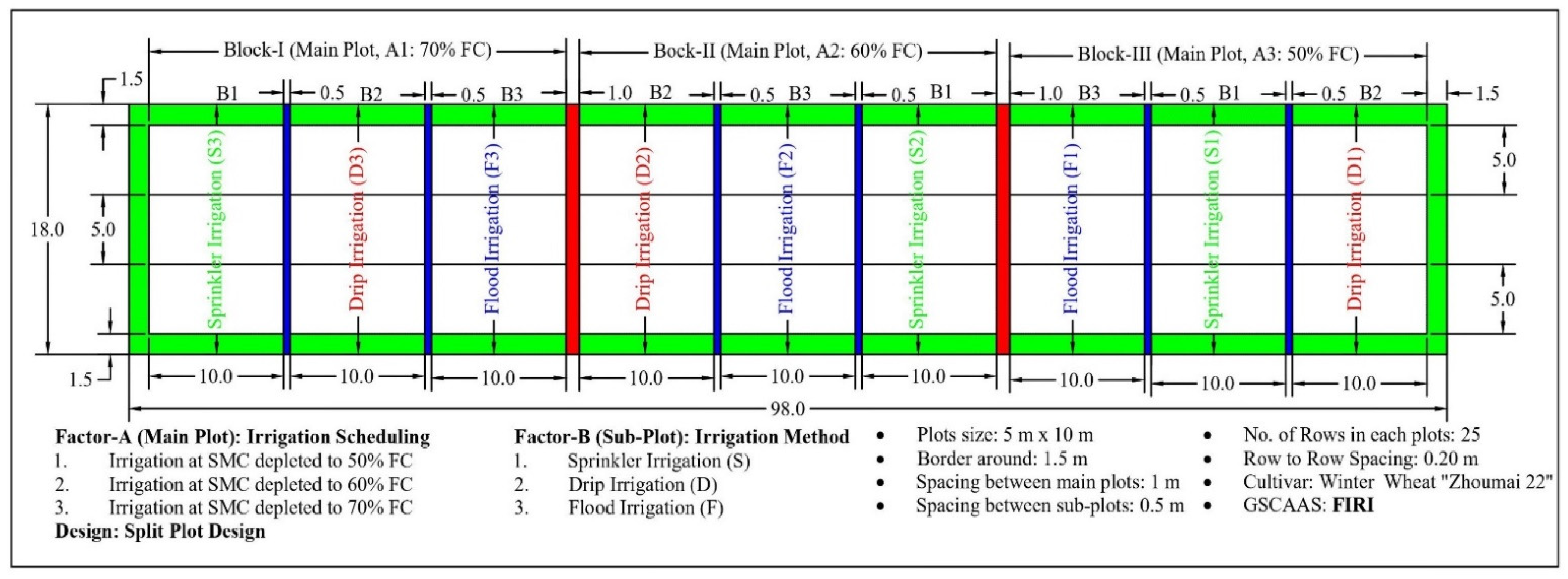
2.1. Site Description and Experimental Design

Field experiments were conducted over two winter wheat seasons from October to June 2016–2018 at the Qiliying field experimental station of the Farmland Irrigation Research Institute, Chinese Academy of Agriculture Sciences, Xinxiang City, Henan Province, on the NCP (35°08′ N, 113°45′ E, elevation 81 m). The field is irrigated by groundwater drawn by a pressure-regulated pump and PVC pipeline adjacent to the plot. The seedbed was prepared to a depth of 0.2 m with a tractor-driven rototiller, and soil clods were broken with a harrow to make the field surface uniform and levelled. The basal dose of ammonium nitrate (N), calcium superphosphate (P), and potassium sulfate (K) was broadcasted at the ratio of 4:3:1, respectively, for all treatments [31]. The ammonium nitrate was applied at a rate of 300 kg N ha⁻¹ by manual broadcasting for all treatments, followed by irrigation. On 16 October 2016 and 22 October 2017, seeds of the winter wheat (Triticum aestivum L.) cultivar “Zhoumai 22” were sown with a tractor-drawn seed drill at a rate of 111.1 kg seed/ha⁻¹ with 0.2 m row spacing. Harvesting was carried out manually from a 1 m² area randomly on 6 June 2017 and 2018. The grains were winnowed and sun-dried to a moisture content of 12% [31] and then weighed using a precise digital balance (Ohaus, AX224 Adventurer, Parsippany, NJ, USA). An automatic weather station (Campbell Scientific Ltd., Logan, UT, USA) was installed near the field to collect weather data.

A two-factor split plot design was adopted, with the three irrigation levels set as the main block, i.e., irrigating immediately as the soil moisture declined to 50% (1), 60% (2), and 70% (3) of field capacity (FC). The sub-blocks were the three irrigation methods arranged randomly, i.e., surface drip (D), flood (F), and sprinkler (S) irrigation. In total, there were nine treatments: D1, D2, D3, F1, F2, F3, S1, S2, and S3, as described in Figure 1. The treatments were not replicated, as, if each sub-plot were randomly placed, the pipeline layout would be very complicated in the small area (one plot: 5 m × 10 m). The experimental field had grown winter wheat for many years (about >20 years) before this irrigation experiment; therefore, the farmland is flat and has uniform infertility. The discharge meters (with pressure gauges and valves) were installed in each plot for independent irrigation, which ensured the relative independence of each plot. Moreover, the analysis in the paper was based on regression analysis; therefore, replication was not essential.

Before irrigation, the SWC of the 1 m soil profile was monitored weekly for irrigation using TRIME-PICO (T3/IPH44, IMKO, Ettlingen, Germany) TDR. The soil moisture readings were held inside the tubes at a 0.2 m span up to a 1 m soil profile. Irrigation was determined on the SWC according to the treatment (50%, 60%, or 70% of FC). Precise discharge gauges were installed in each treatment to ensure the precise amount of irrigation. In flood irrigation, a 60 mm depth of water was applied, and 30 mm were applied for drip and sprinkler irrigation methods [32].

Table 1. Irrigation date, number of irrigations, and irrigation amount for all treatments in 2017 and 2018.

	2017			2018
Treatments	Date (Day after Sowing)	Irrigations Times	Amount (mm)	Date (Day after Sowing)	Irrigation Times	Amount (mm)
S1	174, 180, 202, 214	4	120	163, 174, 199	3	90
D1	174, 180, 207, 214	4	120	163, 174, 199	3	90
F1	174, 202, 214	3	180	174	1	60
S2	174, 180, 193, 207, 214	5	150	163, 174, 185, 199	4	120
D2	174, 180, 193, 207, 214	5	150	163, 174, 185, 199	4	120
F2	174, 180, 207, 214	4	240	174, 192	2	120
S3	174, 180, 193, 202, 207, 214	6	180	163, 174, 185, 192, 199	5	150
D3	174, 180, 193, 202, 207, 214	6	180	163, 174, 185, 192, 199	5	150
F3	174, 180, 193, 202, 207	5	300	174, 185, 199	3	180

presents the irrigation date, number of irrigations, and irrigation amount for each treatment in both growing seasons.

2.2. Model Description

The FAO crop model, AquaCrop [18], predicts the possible yields of the main herbaceous crops in terms of water utilization under rain-fed, supplemental, deficit, and full irrigation scenarios. The AquaCrop model is water-driven. The model simulates the biomass growth as a linear function of transpiration through the WP, the biomass per unit of water transpired [33]. AquaCrop is suitable for use in distinct areas and weather under normal conditions. In the present study, simulations were carried out in thermal time, calendar time, and in daily time steps. The AquaCrop model simulates the daily biomass production as follows:

$${\mathrm{B}}_{\mathrm{i}}={\mathrm{WP}}^{*}\sum \frac{{\mathrm{T}}_{\mathrm{ri}}}{{\mathrm{ET}}_{\mathrm{oi}}}$$

(1)

where B_i is the daily aboveground biomass, T_ri is the daily crop transpiration (mm), ET_oi is the daily reference evapotranspiration, and WP^* is the crop water productivity normalized for both evaporative demand and atmospheric CO₂ [34].

The AquaCrop model calculates canopy cover from crop emergence to senescence. Therefore, canopy cover is the base for simulating T_r in the model. Simulating the daily water balance, the AquaCrop model separates T_r and soil evaporation. Hence, water stress causes leaf senescence at the late growth stages and results in a lower T_r. Canopy cover is an important component in AquaCrop because its growth, aging, and senescence influence the transpiration and, hence, the simulated biomass. The growth of canopy cover is described as [35], where Equations (2) and (3) describe the increase and decrease in canopy cover, respectively.

$$\mathrm{CC}={\mathrm{CC}}_0{\mathrm{e}}^{\mathrm{tCGC}}$$

(2)

$$\mathrm{CC}={\mathrm{CC}}_{\mathrm{X}}-\left({\mathrm{CC}}_{\mathrm{X}}-{\mathrm{CC}}_0\right){\mathrm{e}}^{-\mathrm{tCGC}}$$

(3)

where CC is the canopy cover at time t, CC₀ is the initial CC, CC_X is the maximum canopy cover, CGC is the canopy growth coefficient in fraction per day, and t is the time in days.

Grain dry matter yield was simulated as the product of biomass and the harvest index, and from the wheat flowering stage the harvest index grows linearly with time up to the physiological maturity stage. Crop reactions to water deficit were simulated under four main plant processes: canopy development, stomatal control of transpiration, canopy senescence, and the harvest index. The harvest index could be adjusted positively or negatively, depending on the severity, timing, and duration of stress. The AquaCrop model simulates a soil water balance that contains incoming water (rainfall, irrigation, and capillary rise) and outgoing (deep percolation, runoff, evaporation, and transpiration) water fluxes and change in soil water content at the root zone boundaries.

2.3. Crop and Soil Parameters

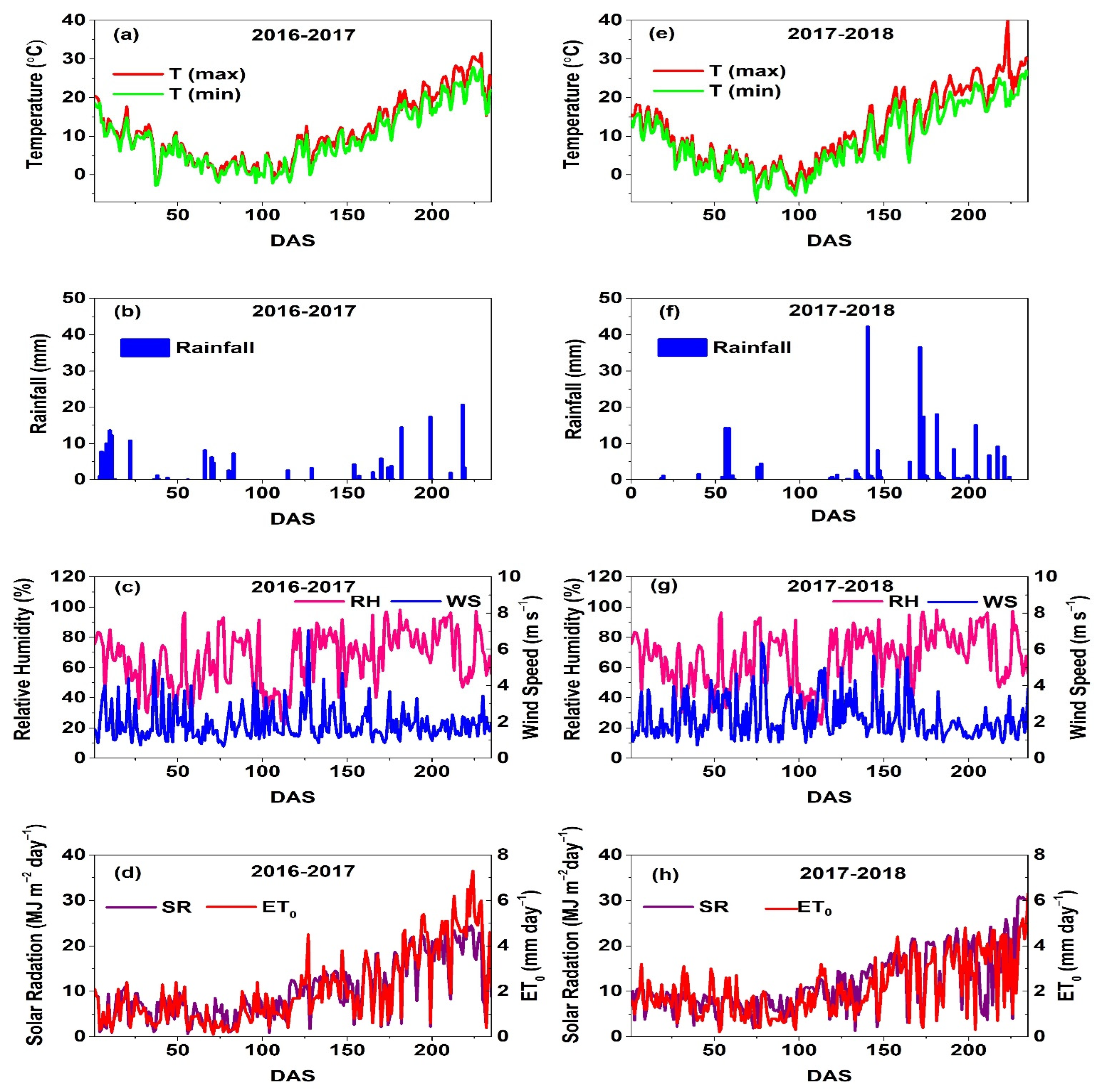
The ET_C for each treatment was determined using the soil water balance equation Hillel [36].

$${\mathrm{ET}}_{\mathrm{C}}=\mathrm{P}+\mathrm{I}+\mathrm{U}-{\mathrm{D}}_{\mathrm{w}}-\mathrm{R}\pm \mathsf{\Delta }\mathrm{S}$$

(4)

where ET_C is the crop evapotranspiration, P is the rainfall; I is the amount of irrigation, U is the upward capillary rise from the soil profile below 1 m, D_w is the downward flux (drainage) beneath the 1 m soil profile, R is the surface runoff, and ΔS is the change in soil water storage in the 1 m soil profile. U is considered to be negligible due to the groundwater table being 30 m below the surface. Downward flux (D_w) was measured following [37]; runoff (R) was neglected owing to suitable bund height (0.25 m) around the sub-blocks. According to [38], WP (kg m⁻³) was estimated by dividing the grain yield by the ET_C.

Leaf area was measured weekly after the re-greening stage by removing the 0.20 m row of plants and selecting ten plants randomly from each treatment. The leaf area index (LAI) was measured as [39].

$$\mathrm{Leaf}\mathrm{area}\mathrm{per}\mathrm{plant}\left(\mathrm{A}\right)=\frac{{{\displaystyle \sum }}_{\mathrm{i}=1}^{\mathrm{n}}{\mathrm{A}}_{\mathrm{i}}}{\mathrm{n}}=\frac{{{\displaystyle \sum }}_{\mathrm{i}=1}^{\mathrm{n}}\left[{{\displaystyle \sum }}_{\mathrm{j}=1}^{\mathrm{m}}\left({\mathrm{L}}_{\mathrm{j}}\times {\mathrm{W}}_{\mathrm{j}}\right)\times 0.80\right]}{\mathrm{n}}$$

(5)

$$\mathrm{LAI}=\frac{\mathrm{A}\times \mathrm{N}}{\mathrm{s}}$$

(6)

where n is the number of plant samples taken for leaf area measurement (n = 10), ${\mathrm{A}}_{\mathrm{i}}=[{\displaystyle \sum }_{\mathrm{j}=1}^{\mathrm{m}}\left({\mathrm{L}}_{\mathrm{j}}\times {\mathrm{W}}_{\mathrm{j}}\right)\times 0.8]$ is the leaf area of the i^th plant, m is the number of leaves of the i^th plant, L_j and W_j are the length and widest width of the j^th leaf of the i^th plant in cm, A is m², N is the number of plant tillers per meter of row length, and S is the space between two plant rows in m (S = 0.20 m).

The LAI was converted into fractional ground canopy cover using the following equation [40].

$$\mathrm{CC}=\left(1-{\mathrm{e}}^{-0.65\times \mathrm{LAI}}\right)$$

(7)

Crop parameters, such as growth stage, seedling emergence date, maximum canopy cover, duration of flowering, initialization of senescence, and maturity, were observed for each treatment. Moreover, the canopy decline coefficient, crop coefficient for transpiration at full canopy cover, soil water depletion thresholds for inhibition of leaf growth, and stomatal conductance, an expedition of canopy senescence, were referenced from [40]. These parameters were assumed to be valid for a wide range of conditions and not limited to a given crop cultivar [41].

The soil physical properties, i.e., soil texture, field capacity (θ_FC), permanent wilting point (θ_PWP), water content at saturation (θ_sat), and saturated hydraulic conductivity (K_sat) were determined at intervals of 0.2 m from the soil surface to a depth of 1 m (

Table 2. Soil physical characteristics of the experimental site.

Depth (m)	Particle Size Distribution			Texture	θFC (Vol %)	θPWP (Vol %)	θsat (Vol %)	Ksat (mm day−1)	CN
	Clay (%)	Silt (%)	Sand (%)
0–0.2	3.8	43.1	53.1	Sandy Loam	21.8	7.4	36.7	1191.1	65
0.2–0.4	6.6	45.4	48.0	Sandy Loam	22.9	8.3	40.2	937.1
0.4–0.6	6.0	48.4	45.6	Sandy Loam	23.6	8.3	39.8	982.3
0.6–0.8	4.6	47.4	48.0	Sandy Loam	23.1	7.9	38.2	1097.8
0.8–1.0	1.6	16.9	81.5	Loamy Sand	13.2	4.5	29.9	2288.2

Note: θ_FC: Field capacity; θ_PWP: Permanent wilting point; θ_sat: saturated water content at saturation; K_sat: Hydraulic conductivity at saturation; CN: curve number (for hydrologic soil group “B” classified based on the K_sat of the top horizon).

). The soil particle size proportion, as determined by the hydrometer method, and soil texture were determined using a soil textural triangle. The θ_FC, θ_PWP, θ_sat, and K_sat of the soil were estimated with the soil hydraulic properties calculator for a predetermined soil particle size distribution [42]. For proper field management, the curve number of 65 was used as a default value. No impervious soil layer was observed in the field, which restricts the growth and expansion of roots. The physical characteristics and chemical properties of the soil in the experimental site are shown in Table 2 and

Table 3. Soil chemical properties of the experimental site.

Depth (m)	pH	EC (µs cm−1)	Available N (mg kg−1)	Available P (mg kg−1)	Available K (mg kg−1)	Organic Carbon (g kg−1)
0–0.2	8.5	132.4	44.6	16.1	128.8	1.9
0.2–0.4	8.6	140.3	44.6	15.0	126.2	1.6
0.4–0.6	8.7	146.3	42.7	14.4	128.3	1.0
0.6–0.8	8.8	155.6	41.8	14.3	124.1	0.7
0.8–1.0	8.9	147.6	41.8	15.3	122.1	0.5

, respectively.

Table 4. Crop and soil parameters used to calibrate AquaCrop model.

Crop Parameters	Value	Unit	Determination
Base temperature	0	°C	Calibrated
Upper temperature	35	°C	Calibrated
Canopy growth coefficient (CGC): Increase in CC per day	0.10	%/day	Calibrated
Canopy decline coefficient (CDC): decrease in CC per day	0.831	%/day	Calibrated
Maximum canopy cover (CCx)	99	%	Measured
Normalized water productivity (WP*)	16	g/m2	Calibrated
Reference harvest index (HIo)	0.55	-	Calibrated
Upper threshold for canopy expansion (Pupper)	0.25	TAW%	Calibrated
Lower threshold for canopy expansion (Plower)	0.60	TAW%	Calibrated
Minimum rooting depth (m)	0.30	m	Default
Maximum rooting depth (m)	1.0	m	Measured
Canopy senescence stress coefficient (Pupper)	0.65	TAW %	Calibrated
Shape factor describing root zone expansion	1.5	-	Calibrated
Crop coefficient when canopy is complete but prior to senescence (Kcb,Trx)	1.10	-	Calibrated
Senescence stress coefficient curve shape	3.0	-	Calibrated
The maximum allowable increase of specified HI	15	%	Calibrated
Minimum air temperature below which pollination starts to fail	5	°C	Calibrated
Maximum air temperature above which pollination starts to fail	35	°C	Calibrated
Water use efficiency normalized for ET0 and CO2 during yield formation	100	%	Calibrated
Fertility stress a	Calibrated	-	Calibrated
Time from sowing to emergence	10	Days	Measured
Time to reach a maximum canopy cover	185	Days	Measured
Time to reach a maximum rooting depth	215	Days	Measured
Time from sowing to start senescence	215	Days	Measured
Time from sowing to flowering	195	Days	Measured
Flowering stage duration	10	Days	Measured

^a Fertility stress is the indicator which varies from 0%, when soil fertility is non-limiting, to 100%, when crop production is unfeasible due to fertility stress. In the “determination” column, “calibrated” indicates that the value was calibrated using the 2016–2017 measured data. “Measured” indicates measured data, and “default” indicates that the value was adopted from the AquaCrop model.

presents the crop and soil parameters used for model calibration. The agricultural soil of the experimental site is mainly an alluvial soil [43] related to Ochri-Aquic Cambosols [44].

The model was calibrated using the observed data from the 2016–2017 growing season as the model input, and then the model simulated the output values (canopy cover, grain yield, biomass, SWC, ET_C, and WP). Afterward, the simulated values were compared with the observed canopy cover, grain yield, biomass, SWC, ET_C, and WP from the field. Disagreement between the observed and simulated data was reduced through trial and error, i.e., a particular reference variable was selected at a time, and we fine-tuned only those parameters that were recognized to affect the reference variable. This was done iteratively, to reduce the variation between the observed and predicted values individually for each treatment.

2.4. Climate Data

AquaCrop model simulations require daily weather data such as minimum and maximum air temperature, reference crop evapotranspiration (ET₀), rainfall, and mean annual CO₂ concentration. ET₀ was estimated using the ET₀ calculator [45], taking into account the daily maximum and minimum temperature, wind speed at 2 m height above the ground surface, solar radiation, and mean relative humidity (RH). The mean annual CO₂ concentration was adopted as the default atmospheric CO₂ concentration from the Mauna Loa observatory records in Hawaii from 1902–2099. An automatic weather station (Campbell Scientific Ltd., Logan, UT, USA) is equipped with a reed switch anemometer, windvane, pyranometer, temperature and relative humidity probe, barometric sensors, and tipping bucket rain gage adjacent (20 m away) to the experimental field. The maximum and minimum temperature (°C) variation, rainfall depth (mm), ET₀ (mm)_, relative humidity (%), wind speed (m s⁻¹), and solar radiation (MJ m⁻² day⁻¹) during the two experimental winter wheat seasons are shown in Figure 2.

2.5. Criteria for Model Evaluation

During both the calibration and validation processes, the AquaCrop model simulations for winter wheat canopy cover, grain yield, biomass, SWC, ET_C, and WP were compared with the observed values from the field experiment. Statistics were used to validate the goodness of fit between the simulated and observed values. Thus, the prediction error (P_e), coefficient of residual mass (CRM), coefficient of determination (R²), root-mean-square error (RMSE), normalized root-mean-square error (NRMSE), and Willmott [46] index of agreement (d) were used as the error statistics to evaluate both the calibration and validation results of the model. The CRM illustrated the tendency of the model to over or underestimate the observed data [47]. The R² value measured the model predictive strength. P_e, RMSE, and NRMSE determined the deviation or model error simulations. In the current study, the model output (canopy cover, grain yield, biomass, SWC, ET_C, and WP) was treated as the model performance, and the following statistical parameters were determined to evaluate the model performance.

$${\mathrm{P}}_{\mathrm{e}}=\frac{\mathrm{Simulated}-\mathrm{Observed}}{\mathrm{Observed}}\times 100$$

(8)

$$\mathrm{CRM}=1-\frac{{{\displaystyle \sum }}_{\mathrm{i}=1}^{\mathrm{n}}{\mathrm{S}}_{\mathrm{i}}}{{{\displaystyle \sum }}_{\mathrm{i}=1}^{\mathrm{n}}{\mathrm{O}}_{\mathrm{i}}}$$

(9)

$${\mathrm{R}}^2={\left[\frac{\sum ({\mathrm{O}}_{\mathrm{i}}-\overline{\mathrm{O}})\left({\mathrm{S}}_{\mathrm{i}}-\overline{\mathrm{S}}\right)}{\sqrt{\sum {\left({\mathrm{O}}_{\mathrm{i}}-\overline{\mathrm{O}}\right)}^2\sum {\left({\mathrm{S}}_{\mathrm{i}}-\overline{\mathrm{S}}\right)}^2}}\right]}^2$$

(10)

$$\mathrm{RMSE}=\sqrt{\frac{\sum {\left({\mathrm{S}}_{\mathrm{i}}-{\mathrm{O}}_{\mathrm{i}}\right)}^2}{\mathrm{n}}}$$

(11)

$$\mathrm{NRMSE}=\frac{1}{\overline{\mathrm{O}}}\sqrt{\frac{\sum {\left({\mathrm{S}}_{\mathrm{i}}-{\mathrm{O}}_{\mathrm{i}}\right)}^2}{\mathrm{n}}}\times 100$$

(12)

$$\mathrm{d}=1-\frac{{{\displaystyle \sum }}_{\mathrm{i}=1}^{\mathrm{n}}{\left({\mathrm{O}}_{\mathrm{i}}-{\mathrm{S}}_{\mathrm{i}}\right)}^2}{\sum {(\left|{\mathrm{S}}_{\mathrm{i}}-\overline{\mathrm{O}}\right|+\left[{\mathrm{O}}_{\mathrm{i}}-\overline{\mathrm{O}}\right])}^2}$$

(13)

where S_i and O_i are simulated and observed data, Ō is the mean value of O_i, and N is the number of observations. A positive CRM value indicates that the model underestimated the observed data, while a negative value indicates that the model overestimated the observed data. R² and the d-index show agreement with values approaching one; P_e and RMSE close to zero were indicators of better model performance. The simulation was considered excellent if NRMSE < 10%, good if 10% < NRMSE < 20%, fair if 20% < NRMSE < 30%, and poor if NRMSE > 30% [21].

3. Results

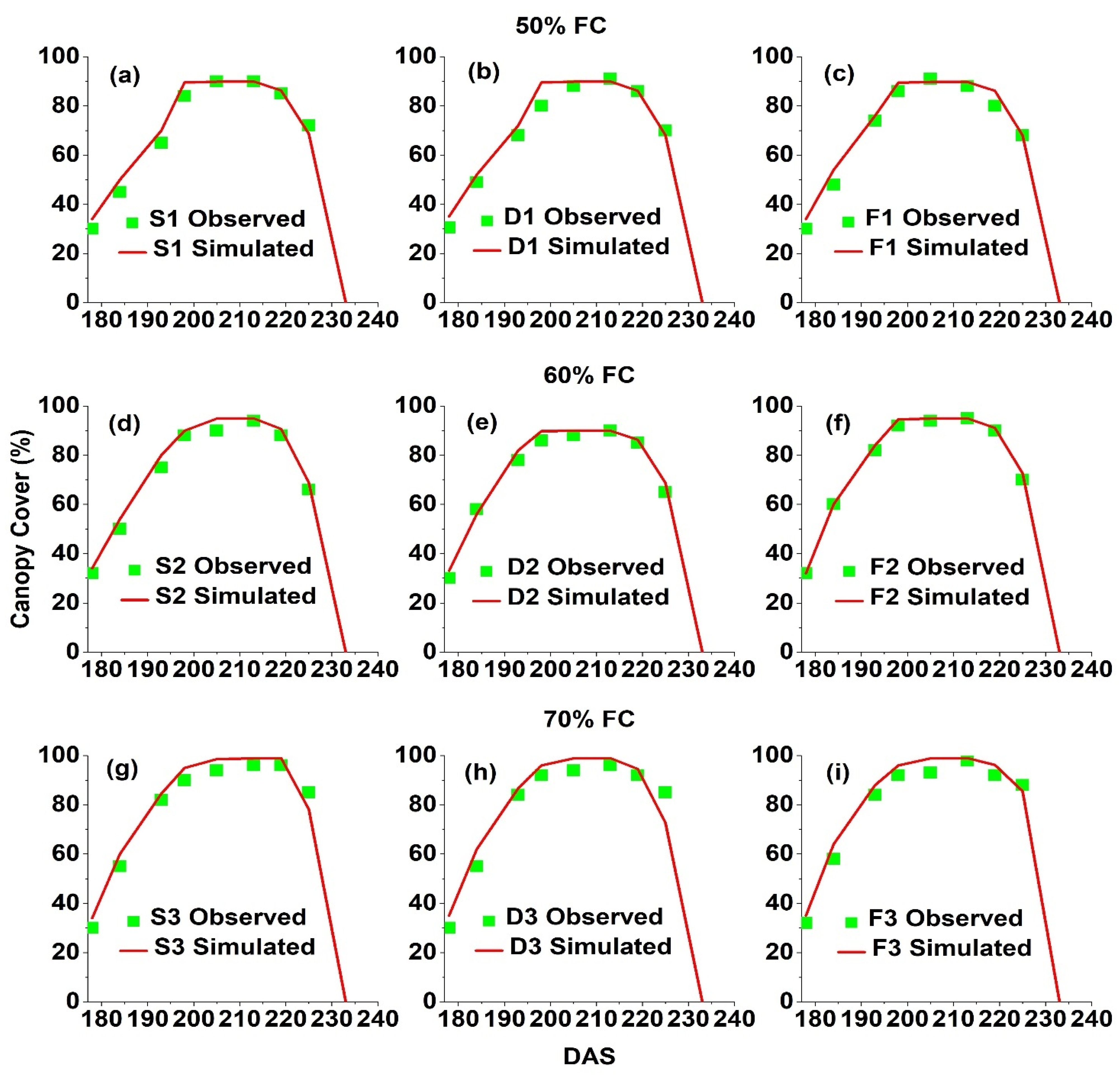
3.1. AquaCrop Model Calibration Results

The simulated values of canopy cover, grain yield, biomass, SWC, ET_C, and WP agreed well with the observed data in the calibration process (Figure 3 and Figure 4;

Table 5. Calibration results of canopy cover and grain yield of winter wheat during the 2016–2017 season.

	Canopy Cover (%)									Grain Yield (t ha−1)
	50% FC			60% FC			70% FC			50% FC			60% FC			70% FC
Irrigation Methods	O	S	Pe (%)	O	S	Pe (%)	O	S	Pe (%)	O	S	Pe (%)	O	S	Pe (%)	O	S	Pe (%)
Sprinkler	70.13	72.30	3.10	72.88	75.94	4.20	78.50	81.03	3.22	8.56	8.69	1.52	9.19	8.94	−2.72	9.10	9.33	2.53
Drip	70.31	72.85	3.61	72.50	74.49	2.74	78.50	80.61	2.69	8.48	8.76	3.30	9.67	9.63	−0.41	9.43	9.68	2.69
Flood	70.63	73.40	3.93	76.88	78.03	1.50	79.63	82.84	4.03	8.29	8.52	2.77	9.10	8.88	−2.42	8.95	9.22	3.02
CRM	−0.04			−0.03			−0.03			−0.03			0.02			−0.03
RMSE	2.51			2.21			2.66			0.22			0.19			0.25
NRMSE (%)	3.57			2.98			3.37			2.65			2.10			2.75

FC: field capacity; O: observed; S: simulated; P_e: prediction error.

,

Table 6. Calibration result of biomass and soil water content (SWC) for different irrigation strategies in 2016–2017.

	Biomass (t ha−1)									SWC (mm)
	50% FC			60% FC			70% FC			50% FC			60% FC			70% FC
Irrigation Methods	O	S	Pe (%)	O	S	Pe (%)	O	S	Pe (%)	O	S	Pe (%)	O	S	Pe (%)	O	S	Pe (%)
Sprinkler	17.22	17.55	1.92	18.47	18.86	2.11	18.61	19.19	3.12	196	201	2.60	209	212	1.20	221	227	3.0
Drip	16.87	17.21	2.02	18.10	18.55	2.49	18.38	18.76	2.07	215	232	7.73	208	210	0.55	212	221	4.1
Flood	17.27	18.00	4.53	19.31	19.48	0.88	19.77	20.22	2.28	223	231	3.72	275	283	3.13	298	311	4.3
CRM	−0.03			−0.02			−0.02			−0.10			−0.02			−0.04
RMSE	0.53			0.36			0.48			11.12			5.21			9.72
NRMSE (%)	3.10			1.92			2.52			5.30			2.30			4.0

FC: field capacity; O: observed; S: simulated; P_e: prediction error.

,

Table 7. Soil water balance in the top one-meter soil profile during the 2016–2017 growing season.

	50% FC			60% FC			70% FC
	Sprinkler	Drip	Flood	Sprinkler	Drip	Flood	Sprinkler	Drip	Flood
Irrigation I (mm)	120	120	180	150	150	240	180	180	300
Precipitation P (mm)	185	185	185	185	185	185	185	185	185
Downward flux Dw (mm)	18	18	27	23	23	36	27	27	60
Change in soil water storage ΔS (mm)	146	147	105	150	170	98	145	155	78
Observed ETC (mm)	433	434	443	463	483	487	483	493	503
Simulated ETC (mm)	446	437	454	450	477	483	493	496	502

FC: field capacity.

and

Table 8. Calibration results of crop evapotranspiration ET_c and water productivity WP in 2016–2017.

	ETC (mm)									WP (kg m−3)
	50% FC			60% FC			70% FC			50% FC			60% FC			70% FC
Irrigation Methods	O	S	Pe (%)	O	S	Pe (%)	O	S	Pe (%)	O	S	Pe (%)	O	S	Pe (%)	O	S	Pe (%)
Sprinkler	433	446	3.10	463	456	−2.81	483	493	2.10	1.98	1.95	−1.66	1.98	1.99	0.51	1.88	1.89	0.66
Drip	434	437	1.00	483	477	−1.24	493	496	0.60	1.96	2.01	2.31	2.00	2.02	1.0	1.91	1.95	2.22
Flood	443	454	2.50	487	483	−0.84	503	502	−0.30	1.87	1.88	0.36	1.86	1.84	−1.1	1.78	1.84	3.24
CRM	−0.02			0.01			−0.01			0.00			0.00			−0.02
RMSE	10.16			5.83			6.10			0.03			0.02			0.04
NRMSE (%)	2.33			1.22			1.23			1.68			0.90			2.26

FC: field capacity; O: observed; S: simulated; P_e: prediction error.

). The calibrated results show that the model slightly overestimated the canopy cover at all irrigation levels (Figure 3a–i). At the 50% FC level (Figure 3a–c), the maximum canopy cover was lower compared with the 60% FC (Figure 3d–f) and 70% FC (Figure 3g–i), while there was no substantial difference measured between the 60% FC and 70% FC for maximum canopy cover. The average canopy cover during the model calibration at 50%, 60%, and 70% FC ranged from 72.3–73.4%, 74.49–78.03%, and 80.61–82.84%, respectively (Table 5), whereas the prediction error for canopy cover varied from 1.50% (F2) to 4.20% (S2). The negative CRM value (−0.03 to −0.04) illustrated that the model slightly overestimated the canopy cover during the model calibration. The RMSE and NRMSE observed at 50%, 60%, and 70% FC were 2.51%, 2.21%, and 2.66% and 3.57%, 2.98%, and 3.37%, respectively. The model slightly overestimated the canopy cover during the model calibration. The R² and d-index between measured and simulated canopy cover were 0.98 and 0.90, respectively (Figure 4a).

The simulated grain yield varied from 8.52 t ha⁻¹ (F1) to 9.68 t ha⁻¹ (D3) (Table 5). The prediction error for grain yield ranged from −2.72% (S2) to 3.30% (D1). The CRM values at 50%, 60%, and 70% FC for grain yield were −0.03, 0.02, and −0.03, respectively. The RMSE for grain yield ranged from 0.19 (60% FC) to 0.25 t ha⁻¹ (70% FC), while the NRMSE for grain yield varied from 2.10 (60% FC) to 2.75% (70% FC). The R² and d-index for grain yield were 0.80 and 0.92, respectively, combined for all treatments (Figure 4b).

The simulated biomass ranged from 17.21 t ha⁻¹ (D1) to 20.22 t ha⁻¹ (F3), respectively (Table 6). The prediction error for biomass ranged from 0.88% (F2) to 4.53% (F1). The CRM value at 50%, 60%, and 70% FC for biomass was −0.03, −0.02, and −0.02, respectively. The RMSE for biomass ranged from 0.36 (60% FC) to 0.53 t ha⁻¹ (50% FC), while the NRMSE for biomass varied from 1.92 (60% FC) to 3.10% (50% FC). The R² and d-index were 0.96 and 1, combined for all treatments (Figure 4c). The calibration results for the SWC of the soil profile (0–1 m) are presented in Table 6. The minimum SWC was simulated in S1 (201 mm) and the maximum in F3 (311 mm). The highest prediction error for the SWC was observed at the water stress irrigation level (50% FC) and the minimum in the moderate irrigation level (60% FC) treatments. The model overestimated the SWC at all irrigation levels. The RMSE and NRMSE for SWC varied from 5.21–11.12 mm and 2.3–5.3%, respectively. A close match was determined between the observed and simulated values of the SWC. The R² and d-index between the observed and simulated SWC combined for all treatments were 0.98 and 0.98, respectively (Figure 4d).

The soil water balance during the growing season of 2016–2017 is presented in Table 7. Flood irrigation compared with sprinkler and drip irrigation received a higher amount of water during the entire season. Therefore, we observed a higher downward flux in flood irrigation compared with sprinkler and drip irrigation at all irrigation levels. A change in soil water storage was observed at a maximum in the drip irrigation at 60% FC (170 mm) and at a minimum in the flood irrigation at 70% FC (78 mm). The observed ET_C and simulated ET_C followed the trend of 70% FC > 60% FC > 50% FC.

The calibration results for ET_C and WP are presented in Table 8. The highest prediction error for ET_C was observed at the water stress irrigation level (50% FC) and the minimum in the moderate irrigation level (60% FC) treatments. The model underestimated the ET_C at 60% FC only. The RMSE and NRMSE for ET_C varied from 5.83–10.16 mm and 1.22–2.33%, respectively. The simulated WP fluctuated from 1.84 kg m⁻³ (F2 and/or F3) to 2.02 kg m⁻³ (D2). The CRM and RMSE for WP were: 50% FC, 0.00 and 0.03 kg m⁻³; 60% FC, 0.00 and 0.02 kg m⁻³; and 70% FC, –0.02 and 0.04 kg m⁻³, respectively. The NRMSE at 50%, 60%, and 70% FC was 1.68, 0.90, and 2.26%, respectively. The R² and d-index between the observed and simulated ET_C and WP combined for all treatments were 0.89, 0.97, and 0.83 and 1.0, respectively (Figure 4e,f).

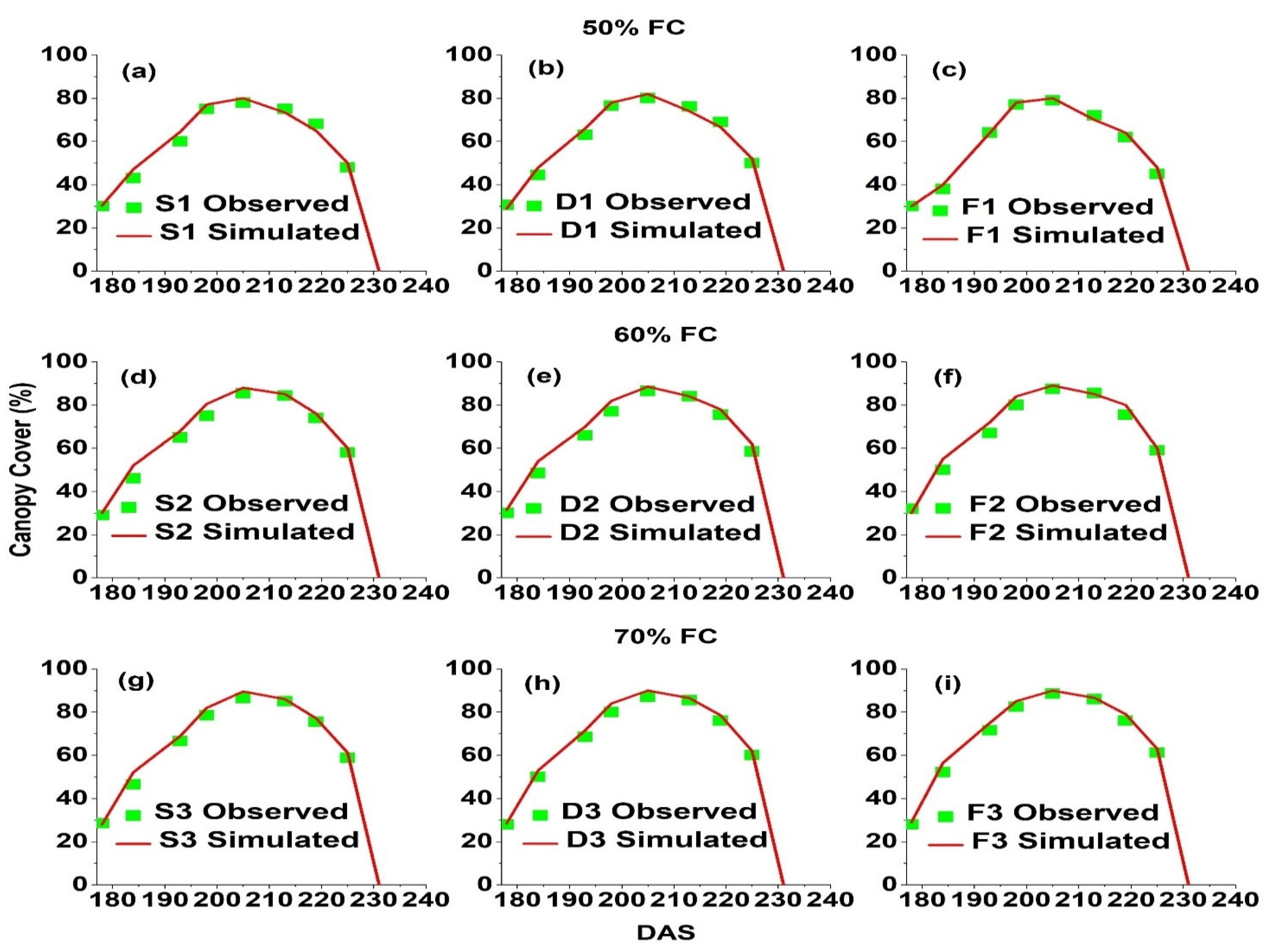
3.2. AquaCrop Model Validation Results

The simulated and observed canopy cover, grain yield, biomass, SWC, ET_C, and WP were in close agreement (Figure 5 and Figure 6;

Table 9. Validation results of canopy cover and grain yield of winter wheat during the 2017−2018 season.

	Canopy Cover (%)									Grain Yield (t ha−1)
	50% FC			60% FC			70% FC			50% FC			60% FC			70% FC
Irrigation Methods	O	S	Pe (%)	O	S	Pe (%)	O	S	Pe (%)	O	S	Pe (%)	O	S	Pe (%)	O	S	Pe (%)
Sprinkler	59.63	60.93	2.18	64.60	67.44	4.39	65.73	68.11	3.63	7.94	8.30	4.53	9.04	9.28	2.68	8.95	9.28	3.70
Drip	61.20	61.95	1.23	65.75	68.75	4.56	66.88	69.25	3.55	8.21	8.64	5.24	9.72	9.62	−1.03	9.30	9.35	0.58
Flood	58.38	59.25	1.50	67.10	69.38	3.43	68.24	70.51	3.33	7.13	7.58	6.34	9.10	8.88	−2.38	8.88	8.81	−0.75
CRM	−0.02			−0.04			−0.04			−0.05			0.00			−0.01
RMSE	1.00			2.73			2.35			0.42			0.19			0.20
NRMSE (%)	1.68			4.15			3.50			5.36			2.11			2.18

FC: field capacity; O: observed; S: simulated; P_e: prediction error.

,

Table 10. Validation results of biomass and soil water content (SWC) under different irrigation strategies in 2017−2018.

	Biomass (t ha−1)									SWC (mm)
	50% FC			60% FC			70% FC			50% FC			60% FC			70% FC
Irrigation Methods	O	S	Pe (%)	O	S	Pe (%)	O	S	Pe (%)	O	S	Pe (%)	O	S	Pe (%)	O	S	Pe (%)
Sprinkler	17.10	17.65	3.22	18.17	18.33	0.88	18.46	19.45	5.36	267	283	6.0	292	303	3.71	307	319	3.84
Drip	16.89	17.55	3.91	18.04	18.24	1.11	18.30	18.70	2.19	268	282	5.40	287	299	4.20	282	300	6.40
Flood	16.66	17.50	5.04	19.18	19.54	1.88	19.52	20.0	2.46	265	279	5.13	298	306	2.80	315	328	4.20
CRM	−0.04			−0.01			−0.03			−0.10			−0.04			−0.05
RMSE	0.70			0.26			0.68			14.70			10.50			14.55
NRMSE (%)	4.11			1.38			3.60			5.52			3.60			4.83

FC: field capacity; O: observed; S: simulated; P_e: prediction error.

,

Table 11. Soil water balance in the top one-meter soil profile during 2017–2018 growing season.

	50% FC			60% FC			70% FC
	Sprinkler	Drip	Flood	Sprinkler	Drip	Flood	Sprinkler	Drip	Flood
Irrigation I (mm)	90	90	60	120	120	120	150	150	180
Precipitation P (mm)	259	259	259	259	259	259	259	259	259
Downward flux D (mm)	14	14	6	18	18	18	23	23	27
Change in soil water storage ΔS (mm)	130	132	100	135	145	138	151	138	125
Observed ETC (mm)	465	467	413	496	506	499	537	524	537
Simulated ETC (mm)	470	478	445	500	498	498	523	531	529

FC: field capacity.

and

Table 12. Validation results of crop evapotranspiration (ET_C) and water productivity (WP) in 2017−2018.

	ETC (mm)									WP (kg m−3)
	50% FC			60% FC			70% FC			50% FC			60% FC			70% FC
Irrigation Methods	O	S	Pe (%)	O	S	Pe (%)	O	S	Pe (%)	O	S	Pe (%)	O	S	Pe (%)	O	S	Pe (%)
Sprinkler	465	470	1.0	496	500	0.82	537	523	−2.62	1.71	1.77	3.27	1.82	1.86	2.0	1.67	1.77	6.25
Drip	467	478	2.32	506	498	−1.53	524	531	1.30	1.76	1.81	2.84	1.92	1.93	0.61	1.77	1.76	−0.42
Flood	413	445	7.90	499	498	−0.13	537	529	−1.50	1.73	1.70	−1.51	1.82	1.78	−1.99	1.65	1.67	1.01
CRM	−0.04			0.00			0.01			−0.02			0.00			−0.02
RMSE	20			5.10			10			0.10			0.03			0.10
NRMSE (%)	4.46			1.0			1.90			2.70			1.64			3.61

FC: field capacity; O: observed; S: simulated; P_e: prediction error.

). At 50% FC irrigation scheduling (Figure 5a–c), the maximum canopy cover was moderately lower with respect to 60% FC (Figure 5d–f) and 70% FC (Figure 5g–i). There was no substantial difference observed between 60% FC and 70% FC for maximum canopy cover. The simulated mean canopy cover for 50% FC ranged from 59.25 (F1) to 61.95% (D1), 60% FC from 67.44% (S2) to 69.38% (F2), and 70% FC from 68.11% (S3) to 70.51% (F3) during the model validation, while the model slightly overestimated (−0.04 < CRM < −0.02) the canopy cover (Table 9). The RMSE and NRMSE for mean canopy cover varied from 1% (50% FC) to 2.73% (60% FC) and from 1.68% (50%FC) to 4.15% (60% FC). The R² and d-index between the observed and simulated canopy cover were 0.99 and 0.92, respectively (Figure 6a).

The higher grain yield was simulated in the D2 (9.62 t ha⁻¹) treatment and the lowest grain yield in F1 (7.58 t ha⁻¹) during the validation process, which was satisfactory with the observed data (Table 9). The P_e for grain yield ranged from −2.38% (F2) to 6.34% (F1) during validation. The CRM for grain yield at 50%, 60%, and 70% FC was −0.05, 0.00, and −0.01, respectively. The RMSE for grain yield ranged from 0.19 (60% FC) to 0.42 t ha⁻¹ (50% FC), while the NRMSE for grain yield varied from 2.11 (60% FC) to 5.36% (50% FC). The R² and d-index for grain yield were 0.93 and 0.95 combined for all treatments (Figure 6b).

The above-ground biomass simulation values varied from 17.50 t ha⁻¹ (F1) to 20.0 t ha⁻¹ (F3), which agreed with the observed data (Table 10). The P_e for biomass ranged from 0.88% (S2) to 5.36% (S3) during validation. The CRM for biomass at 50%, 60%, and 70% FC was −0.04, −0.01, and −0.03, respectively. The RMSE for biomass ranged from 0.26 (60% FC) to 0.70 t ha⁻¹ (50% FC), while the NRMSE for biomass varied from 1.38 (60% FC) to 4.11% (50% FC). The R² and d-index of biomass were 0.92 and 1 combined for all treatments (Figure 6c).

The SWC followed the pattern of 70% FC > 60% FC > 50% FC (Table 10). The minimum deviation in SWC was observed at 60% FC, while the maximum deviation was estimated at the water stress irrigation level (50% FC). The CRM for SWC ranged from −0.10 to −0.05, while the RMSE and NRMSE for SWC varied from 10.50–14.70 mm and 3.60–5.52%, respectively. The simulated SWC agreed well with the observed field data_. The R² and d-index for SWC were 0.98 and 0.86 combined for all treatments (Figure 6d).

The rainfall data from the period 1951–2018 (last 67 years) were analyzed and demonstrated that the winter wheat growing season of 2016–2017 was comparatively dry (185 mm) compared with the 2017–2018 normal season (259 mm). Therefore, rainfall plays an essential role in controlling irrigation scheduling and the total depth of irrigation water application; thus, in 2017–2018, winter wheat drip and sprinkler irrigation had one, while flood irrigation had two fewer irrigation events compared with the 2016–2017 winter wheat growing season with the same irrigation schedules (Table 1). In flood irrigation at 70% FC, the highest irrigation dose (180 mm) was applied, while in flood irrigation at 50% FC, only one irrigation dose (60 mm) was applied (Table 11). Drip and sprinkler irrigation received the same amount of water at all irrigation levels. The downward flux and change in soil water storage varied from 6–27 mm and 100–151 mm, respectively. The observed and simulated ET_C fluctuated from 413–537 mm and 445–531 mm, respectively.

The minimum deviation in ET_C was observed at 60% FC, while the maximum deviation was estimated at the water stress irrigation level (50% FC). The CRM for ET_C ranged from −0.04 to 0.01, while the RMSE and NRMSE for ET_C varied from 5.10–20 mm and 1.0–4.46%, respectively. The simulated ET_C agreed well with the observed field data_. The R² and d-index for ET_C were 0.95 and 0.96 combined for all treatments (Figure 6e). The WP ranged from 1.70 kg m⁻³ (F1) to 1.93 kg m⁻³ (D2) during the model validation (Table 12), while the prediction error varied from −1.99% (F2) to 6.25% (S3). The CRM and RMSE were: 50% FC, −0.02 and 0.10 kg m⁻³; 60% FC, 0.00 and 0.03 kg m⁻³; and 70% FC, −0.02 and 0.10 kg m⁻³, respectively. The NRMSE varied from 1.64% (60% FC) to 3.61% (70% FC) during the validation process. The coefficient of determination and d-index for all treatments between the observed and simulated WP were 0.73 and 1, respectively (Figure 6f). The results imply that the AquaCrop model is a supportive tool for simulating the canopy cover, grain yield, biomass, SWC, ET_C, and WP of winter wheat crops under different irrigation schedules and methods on the NCP.

4. Discussion

Relationships were successfully determined for canopy cover, grain yield, biomass, SWC, ET_C, and WP between the predicted and measured values during the calibration and validation of the AquaCrop model. The results reveal that the model efficiently simulated all the variables tested for winter wheat on the NCP. The crop parameters were tuned to simulate the canopy cover, grain yield, biomass, SWC, ET_C, and WP under different irrigation schedules and methods to acquire precise and stable relationships between the observed and simulated values. The calibration datasets from 2016–2017 were consistent with the model validation results from 2017–2018.

The simulated results of canopy development agreed with the observed data, and the trend was generally similar in all treatments. The model slightly overestimated the canopy cover during calibration and in the validation. Accurate canopy cover simulation is essential for optimal AquaCrop performance because it influences crop transpiration and biomass [27]. The canopy cover peaked near to 205 DAS and started decreasing near 225 DAS (Figure 3 and Figure 5). The decrease in canopy cover was steeper at all irrigation levels. The simulated canopy cover was relatively close to the observed canopy cover up to the flowering stage, while it was slightly overpredicted after senescence. The observed canopy cover declined relatively rapidly compared with the simulated canopy cover, which was attributed to the higher atmospheric temperature causing earlier senescence. In AquaCrop, canopy senescence is explained by the CDC. The influence of a higher temperature on canopy cover was not considered; therefore, the model could not simulate the canopy cover precisely at the end of the crop growing period. The influence of water stress and senescence is complicated to fix in the models; therefore, the AquaCrop model overpredicted the results under higher water stress and temperature conditions. The canopy cover was simulated as lower at all irrigation levels in 2017–2018 compared with that of 2016–2017, which was attributed to the slightly late sowing in the 2017–2018 winter wheat season (22 October) compared with that in the 2016–2017 season (15 October). Therefore, the number of growing days was lower in 2017–2018 compared with that in 2016–2017, which prevented the crop from reaching its maximum canopy cover. These results demonstrate that the increase in irrigation amount increased the canopy cover, while the lowest canopy cover was observed in the water stress treatments.

The CRM validation results illustrate that the grain yield and biomass simulated well at 60% FC and 70% FC irrigation schedules compared with that of the water stress treatment (50% FC) in the model. The close match between the observed and simulated grain yield and biomass at 60% and 70% FC was attributed to the higher SWC in higher-frequency irrigation treatments, leading to a better soil environment. Moreover, the higher development of canopy cover influenced transpiration, grain yield, and biomass. Water stress at 50% FC resulted in insufficient root and crop development, which leads to the minimum grain yield and biomass. The negative CRM values indicate that the AquaCrop model slightly overpredicted the biomass at all irrigation levels during the model calibration and validation, which is attributed to the overpredicted canopy cover at all irrigation levels. The R² value between the observed and simulated grain yield and biomass was 0.93 and 0.92, respectively. The d-index for grain yield was 0.95 and for biomass was 1. These results agree with Mkhabela and Bullock [48], who observed an R² of 0.66 and d-index of 0.99 for a winter wheat grain yield simulation using the AquaCrop model. Stricevic, et al. [49] determined an R² value of >0.84 during yield simulation of maize, sunflower (Helianthus annus L.), and sugar beet (Beta vulgaris L.) under both rain-fed and irrigated treatments in the AquaCrop model, while Karunaratne, et al. [34] observed an R² value of 0.72 for Bambara groundnut (Vignea subterranean L. Verdc) yield using the AquaCrop model.

Our results are consistent with those of Andarzian, et al. [50] and Jin, et al. [29], both of which also found that the AquaCrop model can satisfactorily simulate grain yield and biomass under sufficient irrigation. In water-scarce areas or those with deficit irrigation, sprinkler and drip irrigation at 50% FC can produce an adequate grain yield and biomass with the least yield penalty. The presented results closely agree with those of Iqbal, et al. [30], who observed an RMSE, NRMSE, and IoA (index of agreement or d-index) for grain yield of 0.58 Mg ha⁻¹, 11.82%, and 0.95, and for biomass of 0.87 Mg ha⁻¹, 8.62%, and 0.95, respectively, for winter wheat on the NCP.

The AquaCrop model effectively simulated the wetting and drying intervals that result from irrigation events, while it overpredicted the SWC specifically at the water stress level (50% FC) [51]. The model retained the simulated SWC as higher than the PWP, which estimated a higher SWC during dry periods [48]. The SWC was overpredicted for drip irrigation at 50% and 70% FC, which was possibly due to the slightly wetter surfaces covered by drippers between irrigation periods being considered in the model. The model generally overpredicted the SWC and ET_C; however, the results are consistent with those from the observed data. The maximum deviation between the observed and simulated SWC and ET_C was observed at the water stress level (50% FC), while at the moderate irrigation level (60% FC), the deviation was the minimum. A comprehensive study of the SWC profile in the model illustrated that, at the water stress level (50% FC), the SWC was overpredicted in the topsoil layers and underpredicted in the deeper soil layers [27]. The prediction error statistics suggest that the model can effectively simulate the SWC and ET_C at all irrigation levels and confirm that the model could be used to anticipate the water balance and crop water requirement for winter wheat on the NCP. The prediction statistics for the SWC and ET_C are in line with the Iqbal, et al. [30] for winter wheat in the same region. The model overestimated the SWC and ET_C in the water stress treatments (50% FC) during the validation of the model, which might be due to discrepancies in the model for simulating the SWC and ET_C. Moreover, in the water stress treatments (50% FC), the minimum drainage plus irrigation and rainfall lead to the overestimation of the ET_C. Farahani, et al. [27], Hsiao, et al. [40], and Zeleke, et al. [52] also observed that the AquaCrop model significantly overpredicted the SWC under water stress conditions. However, the simulated SWC values were within an acceptable range. The predicted values of the SWC could be compared with those other models for winter wheat. For instance, Yang, et al. [53] reported deviations of 0.43% to −20.4% between the observed and simulated SWC using the DSSAT-CERES-Wheat model, while Fang, et al. [54] estimated an RMSE of 28.5–34.8 mm for the SWC under wheat–maize rotation using the RZWQM2 model in the same area. The AquaCrop model estimated the ET from the soil evaporation (E) and transpiration (T) of the crops. The variation in the WP suggested that there is room for model development in terms of WP estimation, which is dependent upon the accurate simulation of crop ET.

The field measured ET mainly considers crop transpiration, while the simulated ET complies with soil evaporation, which caused the deviation in ET values [55]. The partition of ET into E and T restricts the ineffective consumptive use of E [56], while optimizing the model WP could be achieved by increasing the T compared with E. Moreover, Farahani, et al. [27] argued that soil evaporation simulated by the model is uncertain, owing to the low values of E measured during irrigation, with significant variation in the amount of water applied. Conservative parameters served to estimate E and T, i.e., extraction patterns of water, the coefficient of crop transpiration, and the coefficient of crop decline were less sensitive to the simulated T values. The lower susceptibility of these parameters indicated the lower response to input variables, usually lower than 2% [33,57]. Regardless of the slightly higher deviations in the SWC and ET_C at the water stress level in our results, the AquaCrop model could certainly be used for simulating the SWC and ET_C at all irrigation scheduling levels under all irrigation methods.

Irrigation is indispensable in this region to reduce water stress, and the WP decreased as the irrigation water amount increased; thus, the lower irrigation schedule treatments (60% FC) have a higher WP compared with that of the higher irrigation schedule treatments (70% FC). The simulated WP varied from 1.67 to 1.93 kg m⁻³ during the validation of the model, which agrees with the studies of Jin, et al. [29] and Fang, et al. [58]. The higher WP suggests that the winter wheat cultivars rapidly improved, causing a higher grain yield and improved WP. The WP values were relatively lower in the 2017–2018 winter wheat cropping season because of the higher amount of rainfall (74 mm) compared with 2016–2017, which increased the crop ET_C and decreased the WP. The AquaCrop model overpredicted the grain yield and ET_C at 50% FC, resulting in the higher WP values. The negative CRM value at 50% FC and 70% FC indicate that the model overestimated the WP, while at 60% FC, the CRM value was zero. Similar results were reported by Kumar, et al. [59], who found that the AquaCrop model overpredicted the WP in winter wheat under various irrigation treatments.

Climate change has a very significant effect on food security. Primarily, it inhibits agricultural production by changing the agricultural and ecological habitat. Secondarily, by stressing growth and economics, it hence escalates the need for agricultural commodities [60]. Wheat yield has been severely influenced by climate change globally. Asseng, et al. [61] and Zhao, et al. [62] observed 6% significant yield losses in wheat crops due to climate change. Similarly, Brown [63] observed a 10% decrease in wheat yield and Ray, et al. [64] measured a 3–4% wheat yield reduction under different climates caused by climate change. Svoboda, et al.’s [65] study revealed that, for sustainable winter wheat yields, the availability of water must be ensured. In China, there may be a scarcity of freshwater resources for irrigation, which might result in the conversion of irrigated land to rainfed land and in a decrease in agricultural production [66]. To prevent groundwater overdraft and reduce climate change impacts, water-saving irrigation methods such as drip and sprinkler irrigation systems are being adopted. Sprinkler and drip irrigation has the potential to withstand climate change by reducing groundwater pumping for irrigation, improving crop yield and WP.

Irrigation mainly depends on ground water resources, and the depletion of underground water resources is a major threat for growers and policy makers in terms of sustainable crop production in this region. Moreover, irrigation wells below 100 m were required, which resulted in a sharp decline in ground water [67]. In general, NCP farmers irrigate 3–5 times with a 60 mm depth of water (total water 180–300 mm) to meet the seasonal ET of 450–500 mm [68]. Higher irrigation scheduling (70% FC) increases soil evaporation, deep percolation, and lowers the WP. The simulation results reveal that, following the re-greening stage, irrigation scheduling of 4–5 irrigations of a 30 mm depth (total water 120–150 mm), depending on the seasonal rainfall amount and soil moisture storage, by drip irrigation and sprinkler irrigation was the most effective irrigation schedule to obtain the optimum grain yield, biomass, and WP on the NCP. This would save a significant amount of water resources, avoid the overexploitation of ground water, and increase the cropping area. The results show that drip irrigation followed by sprinkler irrigation was more highly beneficial to achieve a higher grain yield, biomass, and WP at all irrigation scheduling levels. Therefore, it is suggested that the drip irrigation method be employed on the water-scarce NCP to increase grain yield, biomass, and WP. Our findings suggest that the AquaCrop model could be used for simulating the canopy cover, grain yield, biomass, SWC, ET_C, and WP in winter wheat under various irrigation scheduling and irrigation methods. The irrigation methods exhibited no obvious trend in the simulation, while the simulation was more accurate for grain yield and biomass at higher scheduling levels (70% FC and 60% FC) compared with the water stress scheduling (50% FC).

The AquaCrop model is a reliable tool to improve irrigation scheduling strategies under different irrigation methods that produce an optimum grain yield, biomass, and WP. The model is required to be calibrated and validated due to regular changes in the local cultivars grown by the farmers and to obtain the precise forecast results for the local environment. The advantage of forecasting results could only be obtained if it is used properly with known limitations. One salient feature of the AquaCrop model is the “conservative parameters” that are widely feasible under different climatic conditions and crop cultivars [69]. Usually, these parameters perform well in anticipating crop development under adequate water availability. On the contrary, under the water stress scenario (50% FC), there was slight misfit between the observed and simulated values, which probably illustrated the revision of these values; in particular, the threshold for stress might increase the model performance. Future research is required to apply this model for different irrigation strategies to yield sustainability and water saving. Moreover, this study was limited to the winter wheat in the Qiliying field experimental site on the NCP, and further studies might carry out experiments under full and deficit irrigation scheduling to increase the model’s applicability. In addition to this, future studies are recommended to be carried out over different deficit irrigation regimes and measure the crop yield, biomass, and WP relationship. These results provide an opportunity for growers and policy makers to choose an appropriate irrigation scheduling with a suitable irrigation method for winter wheat growing. Moreover, an economic analysis of each irrigation practice is recommended to better consider the economic benefits of each irrigation strategy.

5. Conclusions

The AquaCrop model was calibrated and validated for three crop parameters, i.e., canopy cover, grain yield, and biomass, and three water parameters, i.e., soil water content, ET_C, and WP, under different irrigation schedules and methods using field data from the 2016–2017 and 2017–2018 winter wheat seasons in the pedoclimatic condition of the NCP. The simulated results illustrate that higher irrigation scheduling treatments enhanced the grain yield and biomass compared with those of the water- stress treatments, while the WP was higher at the 60% FC irrigation scheduling level. The model successfully validated the canopy cover, grain yield, biomass, soil water content, ET_C, and WP. Moreover, the results agree with those from the field data, as evidenced by the prediction error values. The foremost benefit of the AquaCrop model is that it demands fewer input data to simulate the canopy cover, grain yield, biomass, and WP compared with other crop models. The slightly higher deviations recorded at the water stress level might be due to a considerable simplification of the model to reduce its complexity. Our results present that the AquaCrop model successfully simulates the canopy cover, grain yield, biomass, soil water content, ET_C, and WP of winter wheat with a higher certainty under different irrigation schedules and irrigation methods in a case study on the NCP. These findings could give some clues for further research aiming at increasing the applicability of the model to different scenarios.

References

1. Zhang, X.; Chen, S.; Liu, M.; Pei, D.; Sun, H. Improved water use efficiency associated with cultivars and agronomic management in the North China Plain. Agron. J. 2005, 97, 783–790. [Google Scholar] [CrossRef]
2. Wang, J.; Wang, E.; Yang, X.; Zhang, F.; Yin, H. Increased yield potential of wheat-maize cropping system in the North China Plain by climate change adaptation. Clim. Chang. 2012, 113, 825–840. [Google Scholar] [CrossRef]
3. IPCC. Climate Change 2021: The Physical Science Basis. In Contribution of Working Group I to the Sixth Assessment Report of the Intergovernmental Panel on Climate Change; Cambridge University Press: Cambridge, UK, 2021. [Google Scholar]
4. Zhang, X.; You, M. Dynamics of soil-water content and water-saving potential in the farmland of Taihang piedmont. Econ. Agric. Res. 1996, 4, 63–68. [Google Scholar]
5. Cao, G.; Han, D.; Song, X. Evaluating actual evapotranspiration and impacts of groundwater storage change in the North China Plain. Hydrol. Process. 2014, 28, 1797–1808. [Google Scholar] [CrossRef]
6. Jha, S.K. Effect of Irrigation Method and Scheduling on Development and Water Utilization in Winter Wheat. Ph.D. Dissertation, Chinese Academy of Agricultural Sciences, Beijing, China, 2018. [Google Scholar]
7. Li, Y. The Northern China needs a water-saving agriculture. Irrig. Drain. 1993, 12, 10–20. [Google Scholar]
8. Zhang, X.; Pei, D.; Hu, C. Conserving groundwater for irrigation in the North China Plain. Irrig. Sci. 2003, 21, 159–166. [Google Scholar] [CrossRef]
9. Manoliadis, O.G. Analysis of irrigation systems using sustainability-related criteria. J. Environ. Qual. 2001, 30, 1150–1153. [Google Scholar] [CrossRef]
10. Chimonyo, V.G.; Wimalasiri, E.M.; Kunz, R.; Modi, A.T.; Mabhaudhi, T. Optimizing traditional cropping systems under climate change: A case of maize landraces and bambara groundnut. Intercrop. Syst. Sustain. Agric. 2020, 4, 562568. [Google Scholar] [CrossRef]
11. Korres, N.E.; Norsworthy, J.K.; Tehranchian, P.; Gitsopoulos, T.K.; Loka, D.A.; Oosterhuis, D.M.; Gealy, D.R.; Moss, S.R.; Burgos, N.R.; Miller, M.R. Cultivars to face climate change effects on crops and weeds: A review. Agron. Sustain. Dev. 2016, 36, 12. [Google Scholar] [CrossRef] [Green Version]
12. Zhang, B.; Fu, Z.; Wang, J.; Zhang, L. Farmers’ adoption of water-saving irrigation technology alleviates water scarcity in metropolis suburbs: A case study of Beijing, China. Agric. Water Manag. 2019, 212, 349–357. [Google Scholar] [CrossRef]
13. Cui, Z.L.; Chen, X.P.; Zhang, F.S.; Shi, L.W.; Li, J.L. Effect of different border lengths on the irrigation homogeneity and soil nitrate-N distribution on wheat field. Chin. J. Eco-Agric. 2006, 14, 82–85. [Google Scholar]
14. Bernstein, L.; Francois, L. Comparisons of drip, furrow, and sprinkler irrigation. Soil Sci. 1973, 115, 73–86. [Google Scholar] [CrossRef]
15. Rötter, R.P.; Palosuo, T.; Kersebaum, K.C.; Angulo, C.; Bindi, M.; Ewert, F.; Ferrise, R.; Hlavinka, P.; Moriondo, M.; Nendel, C. Simulation of spring barley yield in different climatic zones of Northern and Central Europe: A comparison of nine crop models. Field Crops Res. 2012, 133, 23–36. [Google Scholar] [CrossRef]
16. Mabhaudhi, T.; Modi, A.T.; Beletse, Y.G. Parameterisation and evaluation of the FAO-AquaCrop model for a South African taro (Colocasia esculenta L. Schott) landrace. Agric. For. Meteorol. 2014, 192, 132–139. [Google Scholar] [CrossRef]
17. Greaves, G.E.; Wang, Y.M. Assessment of FAO AquaCrop model for simulating maize growth and productivity under deficit irrigation in a tropical environment. Water 2016, 8, 557. [Google Scholar] [CrossRef]
18. Steduto, P.; Hsiao, T.C.; Raes, D.; Fereres, E. AquaCrop-The FAO crop model to simulate yield response to water: I. Concepts and underlying principles. Agron. J. 2009, 101, 426–437. [Google Scholar] [CrossRef] [Green Version]
19. Rötter, R.; Tao, F.; Höhn, J.; Palosuo, T. Use of crop simulation modelling to aid ideotype design of future cereal cultivars. J. Exp. Bot. 2015, 66, 3463–3476. [Google Scholar] [CrossRef] [Green Version]
20. Azam-Ali, S.; Crout, N.; Bradley, R. Perspectives in modelling resource capture by crops. In Resource Capture by Crops; Nottingham University Press: Nottingham, UK, 1994; pp. 125–148. [Google Scholar]
21. Jamieson, P.; Porter, J.; Wilson, D. A test of the computer simulation model ARCWHEAT1 on wheat crops grown in New Zealand. Field Crops Res. 1991, 27, 337–350. [Google Scholar] [CrossRef]
22. Jamieson, P.; Semenov, M.; Brooking, I.; Francis, G. Sirius: A mechanistic model of wheat response to environmental variation. Eur. J. Agron. 1998, 8, 161–179. [Google Scholar] [CrossRef]
23. Stöckle, C.O.; Donatelli, M.; Nelson, R. CropSyst, a cropping systems simulation model. Eur. J. Agron. 2003, 18, 289–307. [Google Scholar] [CrossRef]
24. Jha, P.K.; Kumar, S.N.; Ines, A.V. Responses of soybean to water stress and supplemental irrigation in upper Indo-Gangetic plain: Field experiment and modeling approach. Field Crops Res. 2018, 219, 76–86. [Google Scholar] [CrossRef]
25. Araya, A.; Prasad, P.; Ciampitti, I.; Jha, P. Using crop simulation model to evaluate influence of water management practices and multiple cropping systems on crop yields: A case study for Ethiopian highlands. Field Crops Res. 2021, 260, 108004. [Google Scholar] [CrossRef]
26. Foster, T.; Brozović, N.; Butler, A.; Neale, C.; Raes, D.; Steduto, P.; Fereres, E.; Hsiao, T.C. AquaCrop-OS: An open source version of FAO’s crop water productivity model. Agric. Water Manag. 2017, 181, 18–22. [Google Scholar] [CrossRef]
27. Farahani, H.J.; Izzi, G.; Oweis, T.Y. Parameterization and evaluation of the AquaCrop model for full and deficit irrigated cotton. Agron. J. 2009, 101, 469–476. [Google Scholar] [CrossRef] [Green Version]
28. Dalla Marta, A.; Chirico, G.B.; Falanga Bolognesi, S.; Mancini, M.; D’Urso, G.; Orlandini, S.; De Michele, C.; Altobelli, F. Integrating Sentinel-2 imagery with AquaCrop for dynamic assessment of tomato water requirements in Southern Italy. Agronomy 2019, 9, 404. [Google Scholar] [CrossRef] [Green Version]
29. Jin, X.L.; Feng, H.K.; Zhu, X.K.; Li, Z.H.; Song, S.N.; Song, X.Y.; Yang, G.J.; Xu, X.G.; Guo, W.S. Assessment of the AquaCrop model for use in simulation of irrigated winter wheat canopy cover, biomass, and grain yield in the North China Plain. PLoS ONE 2014, 9, e86938. [Google Scholar] [CrossRef]
30. Iqbal, M.A.; Shen, Y.; Stricevic, R.; Pei, H.; Sun, H.; Amiri, E.; Penas, A.; del Rio, S. Evaluation of the FAO AquaCrop model for winter wheat on the North China Plain under deficit irrigation from field experiment to regional yield simulation. Agric. Water Manag. 2014, 135, 61–72. [Google Scholar] [CrossRef]
31. Gao, Y.; Yang, L.; Shen, X.; Li, X.; Sun, J.; Duan, A.; Wu, L. Winter wheat with subsurface drip irrigation (SDI): Crop coefficients, water-use estimates, and effects of SDI on grain yield and water use efficiency. Agric. Water Manag. 2014, 146, 1–10. [Google Scholar] [CrossRef]
32. Bergaust, L.; Mao, Y.; Bakken, L.R.; Frostegård, Å. Denitrification response patterns during the transition to anoxic respiration and posttranscriptional effects of suboptimal pH on nitrogen oxide reductase in Paracoccus denitrificans. Appl. Environ. Microbiol. 2010, 76, 6387–6396. [Google Scholar] [CrossRef] [Green Version]
33. Geerts, S.; Raes, D.; Garcia, M.; Miranda, R.; Cusicanqui, J.A.; Taboada, C.; Mendoza, J.; Huanca, R.; Mamani, A.; Condori, O.; et al. Simulating Yield Response of Quinoa to Water Availability with AquaCrop. Agron. J. 2009, 101, 499–508. [Google Scholar] [CrossRef]
34. Karunaratne, A.; Azam-Ali, S.; Izzi, G.; Steduto, P. Calibration and validation of FAO-AquaCrop model for irrigated and water deficient bambara groundnut. Exp. Agric. 2011, 47, 509–527. [Google Scholar] [CrossRef]
35. Smith, M.; Steduto, P. Yield response to water: The original FAO water production function. FAO Irrig. Drain. Pap. 2012, 66, 6–13. [Google Scholar]
36. Hillel, D. Environmental Soil Physics: Fundamentals, Applications, and Environmental Considerations; Academic Press: London, UK, 1998. [Google Scholar]
37. Sun, H.-Y.; Liu, C.-M.; Zhang, X.-Y.; Shen, Y.-J.; Zhang, Y.-Q. Effects of irrigation on water balance, yield and WUE of winter wheat in the North China Plain. Agric. Water Manag. 2006, 85, 211–218. [Google Scholar] [CrossRef]
38. Peng, Z.; Zhang, B.; Xu, D.; Cai, J. Optimization of irrigation schedule based on the response relationship of water consumption and yield for winter wheat in North China Plain. Desalination Water Treat. 2018, 118, 26–38. [Google Scholar] [CrossRef]
39. Gao, Y.; Duan, A.; Qiu, X.; Liu, Z.; Sun, J.; Zhang, J.; Wang, H. Distribution of roots and root length density in a maize/soybean strip intercropping system. Agric. Water Manag. 2010, 98, 199–212. [Google Scholar] [CrossRef]
40. Hsiao, T.C.; Heng, L.; Steduto, P.; Rojas-Lara, B.; Raes, D.; Fereres, E. AquaCrop-the FAO crop model to simulate yield response to water: III. Parameterization and testing for maize. Agron. J. 2009, 101, 448–459. [Google Scholar] [CrossRef]
41. Heng, L.K.; Hsiao, T.; Evett, S.; Howell, T.; Steduto, P. Validating the FAO AquaCrop model for irrigated and water deficient field maize. Agron. J. 2009, 101, 488–498. [Google Scholar] [CrossRef] [Green Version]
42. Saxton, K.; Rawls, W.J.; Romberger, J.S.; Papendick, R. Estimating generalized soil-water characteristics from texture. Soil Sci. Soc. Am. J. 1986, 50, 1031–1036. [Google Scholar] [CrossRef]
43. Gong, Z.; Zhang, G.; Chang, Z. Pedogenesis and Soil; Taxonomy Science Press: Beijing, China, 2007. [Google Scholar]
44. Xie, Y.X.; Zhang, H.; Zhu, Y.J.; Li, Z.; Yang, J.H.; Cha, F.N.; Cao, L.; Wang, C.Y.; Guo, T.C. Grain yield and water use of winter wheat as affected by water and sulfur supply in the North China Plain. J. Integr. Agric. 2017, 16, 614–625. [Google Scholar] [CrossRef] [Green Version]
45. FAO. ETo calculator version 3.1. In Evapotranspiration from Reference Surface; FAO, Land and Water Division: Rome, Italy, 2009. [Google Scholar]
46. Willmott, C.J. Some comments on the evaluation of model performance. Bull. Am. Meteorol. Soc. 1982, 63, 1309–1313. [Google Scholar] [CrossRef]
47. Loague, K.; Green, R.E. Statistical and graphical methods for evaluating solute transport models: Overview and application. J. Contam. Hydrol. 1991, 7, 51–73. [Google Scholar] [CrossRef]
48. Mkhabela, M.S.; Bullock, P.R. Performance of the FAO AquaCrop model for wheat grain yield and soil moisture simulation in Western Canada. Agric. Water Manag. 2012, 110, 16–24. [Google Scholar] [CrossRef]
49. Stricevic, R.; Cosic, M.; Djurovic, N.; Pejic, B.; Maksimovic, L. Assessment of the FAO AquaCrop model in the simulation of rainfed and supplementally irrigated maize, sugar beet and sunflower. Agric. Water Manag. 2011, 98, 1615–1621. [Google Scholar] [CrossRef]
50. Andarzian, B.; Bannayan, M.; Steduto, P.; Mazraeh, H.; Barati, M.; Barati, M.; Rahnama, A. Validation and testing of the AquaCrop model under full and deficit irrigated wheat production in Iran. Agric. Water Manag. 2011, 100, 1–8. [Google Scholar] [CrossRef]
51. Hussein, F.; Janat, M.; Yakoub, A. Simulating cotton yield response to deficit irrigation with the FAO AquaCrop model. Span. J. Agric. Res. 2011, 9, 1319–1330. [Google Scholar] [CrossRef] [Green Version]
52. Zeleke, K.T.; Luckett, D.; Cowley, R. Calibration and testing of the FAO AquaCrop model for canola. Agron. J. 2011, 103, 1610–1618. [Google Scholar] [CrossRef]
53. Yang, Y.; Watanabe, M.; Zhang, X.; Zhang, J.; Wang, Q.; Hayashi, S. Optimizing irrigation management for wheat to reduce groundwater depletion in the piedmont region of the Taihang Mountains in the North China Plain. Agric. Water Manag. 2006, 82, 25–44. [Google Scholar] [CrossRef]
54. Fang, Q.; Ma, L.; Yu, Q.; Ahuja, L.; Malone, R.; Hoogenboom, G. Irrigation strategies to improve the water use efficiency of wheat–maize double cropping systems in North China Plain. Agric. Water Manag. 2010, 97, 1165–1174. [Google Scholar] [CrossRef]
55. Katerji, N.; Campi, P.; Mastrorilli, M. Productivity, evapotranspiration, and water use efficiency of corn and tomato crops simulated by AquaCrop under contrasting water stress conditions in the Mediterranean region. Agric. Water Manag. 2013, 130, 14–26. [Google Scholar] [CrossRef]
56. Raes, D.; Steduto, P.; Hsiao, T.C.; Fereres, E. AquaCrop the FAO crop model to simulate yield response to water: II. Main algorithms and software description. Agron. J. 2009, 101, 438–447. [Google Scholar] [CrossRef] [Green Version]
57. Salemi, H.; Soom, M.A.M.; Lee, T.S.; Mousavi, S.F.; Ganji, A.; Yusoff, M.K. Application of AquaCrop model in deficit irrigation management of Winter wheat in arid region. Afr. J. Agric. Res. 2011, 6, 2204–2215. [Google Scholar]
58. Fang, Q.X.; Chen, Y.H.; Li, Q.Q.; Yu, S.Z.; Luo, Y. Effect of irrigation on water use efficiency of winter wheat. Trans. Chin. Soc. Agric. Eng. 2004, 20, 34–39. (In Chinese) [Google Scholar]
59. Kumar, P.; Sarangi, A.; Singh, D.; Parihar, S. Evaluation of AquaCrop model in predicting wheat yield and water productivity under irrigated saline regimes. Irrig. Drain. 2014, 63, 474–487. [Google Scholar] [CrossRef]
60. Raza, A.; Razzaq, A.; Mehmood, S.S.; Zou, X.; Zhang, X.; Lv, Y.; Xu, J. Impact of climate change on crops adaptation and strategies to tackle its outcome: A review. Plants 2019, 8, 34. [Google Scholar] [CrossRef] [Green Version]
61. Asseng, S.; Ewert, F.; Martre, P.; Rötter, R.P.; Lobell, D.B.; Cammarano, D.; Kimball, B.A.; Ottman, M.J.; Wall, G.; White, J.W. Rising temperatures reduce global wheat production. Nat. Clim. Chang. 2015, 5, 143–147. [Google Scholar] [CrossRef]
62. Zhao, C.; Liu, B.; Piao, S.; Wang, X.; Lobell, D.B.; Huang, Y.; Huang, M.; Yao, Y.; Bassu, S.; Ciais, P. Temperature increase reduces global yields of major crops in four independent estimates. Proc. Natl. Acad. Sci. USA 2017, 114, 9326–9331. [Google Scholar] [CrossRef]
63. Brown, L.R. Plan B 3.0: Mobilizing to Save Civilization (Substantially Revised); WW Norton & Company: New York, NY, USA, 2008. [Google Scholar]
64. Ray, D.K.; Gerber, J.S.; MacDonald, G.K.; West, P.C. Climate variation explains a third of global crop yield variability. Nat. Commun. 2015, 6, 5989. [Google Scholar] [CrossRef] [PubMed] [Green Version]
65. Svoboda, N.; Strer, M.; Hufnagel, J. Rainfed winter wheat cultivation in the North German Plain will be water limited under climate change until 2070. Environ. Sci. Eur. 2015, 27, 29. [Google Scholar] [CrossRef] [PubMed] [Green Version]
66. Elliott, J.; Deryng, D.; Müller, C.; Frieler, K.; Konzmann, M.; Gerten, D.; Glotter, M.; Flörke, M.; Wada, Y.; Best, N. Constraints and potentials of future irrigation water availability on agricultural production under climate change. Proc. Natl. Acad. Sci. USA 2014, 111, 3239–3244. [Google Scholar] [CrossRef] [Green Version]
67. Zhou, L.L.; Liao, S.H.; Wang, Z.M.; Wang, P.; Zhang, Y.H.; Yan, H.J.; Gao, Z.; Shen, S.; Liang, X.G.; Wang, J.H. A simulation of winter wheat crop responses to irrigation management using CERES-Wheat model in the North China Plain. J. Integr. Agric. 2018, 17, 1181–1193. [Google Scholar] [CrossRef] [Green Version]
68. Zhang, Y.; Li, C.; Zhou, X.; Moore, B. A simulation model linking crop growth and soil biogeochemistry for sustainable agriculture. Ecol. Model. 2002, 151, 75–108. [Google Scholar] [CrossRef]
69. Raes, D.; Steduto, P.; Hsiao, T.; Fereres, E. AquaCrop Reference Manual; (Version 4.0); FAO: Rome, Italy, 2012; Chapter 3. [Google Scholar]
Figure 1. The field experimental design layout and treatment arrangement.
Agronomy 12 03184 g001
Figure 2. Daily maximum and minimum air temperature (a,e), rainfall (b,f), relative humidity and wind speed (c,g), solar radiation (SR) and reference evapotranspiration (ET0) (d,h) trends on the day after sowing (DAS) during the study period in 2016−2017 and 2017−2018.
Agronomy 12 03184 g002
Figure 3. Calibration results of canopy cover (%) of winter wheat at 50% FC (ac), 60% FC (df), and 70% FC (gi) under the sprinkler, drip, and flood irrigation system in 2016–2017. Note: S1: sprinkler irrigation at 50% FC, D1: drip irrigation at 50% FC, F1: flood irrigation at 50% FC, S2: sprinkler irrigation at 60% FC, D2: drip irrigation at 60% FC, F2: flood irrigation at 60% FC, S3: sprinkler irrigation at 70% FC, D3: drip irrigation at 70% FC, F3: flood irrigation at 70% FC.
Agronomy 12 03184 g003
Figure 4. The relation between observed and simulated values for canopy cover (a), grain yield (b), biomass (c), soil water content SWC (d), crop evapotranspiration ETc (e), and water productivity WP (f) under all treatments in 2016−2017 under model calibration.
Agronomy 12 03184 g004
Figure 5. Validation results of canopy cover (%) of winter wheat at 50% FC (ac), 60% FC (df), and 70% FC (gi) under the sprinkler, drip, and flood irrigation system in 2017–2018. Note: S1: sprinkler irrigation at 50% FC, D1: drip irrigation at 50% FC, F1: flood irrigation at 50% FC, S2: sprinkler irrigation at 60% FC, D2: drip irrigation at 60% FC, F2: flood irrigation at 60% FC, S3: sprinkler irrigation at 70% FC, D3: drip irrigation at 70% FC, F3: flood irrigation at 70% FC.
Agronomy 12 03184 g005
Figure 6. The relation between observed and simulated values for canopy cover (a), grain yield (b), biomass (c), soil water content SWC (d), crop evapotranspiration ETc (e), and water productivity WP (f) under all treatments in 2017−2018 under model validation.
Agronomy 12 03184 g006