


Application and Evaluation of a Simple Crop Modelling Framework: A Case Study for Spring Barley, Winter Wheat and Winter Oilseed Rape over Ireland


Abstract
1. Introduction
2. Materials and Methods
2.1. Context
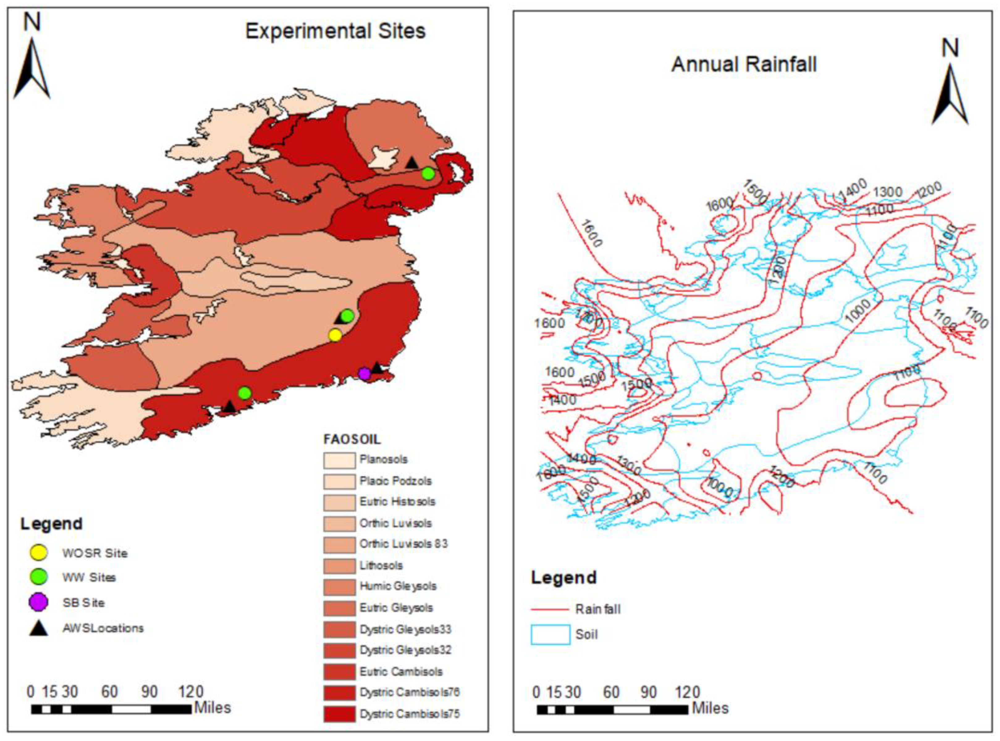
2.2. Study Locations
2.3. Evaluation Data: In Situ
2.4. Site Soil Information
2.5. Meteorlogical Data
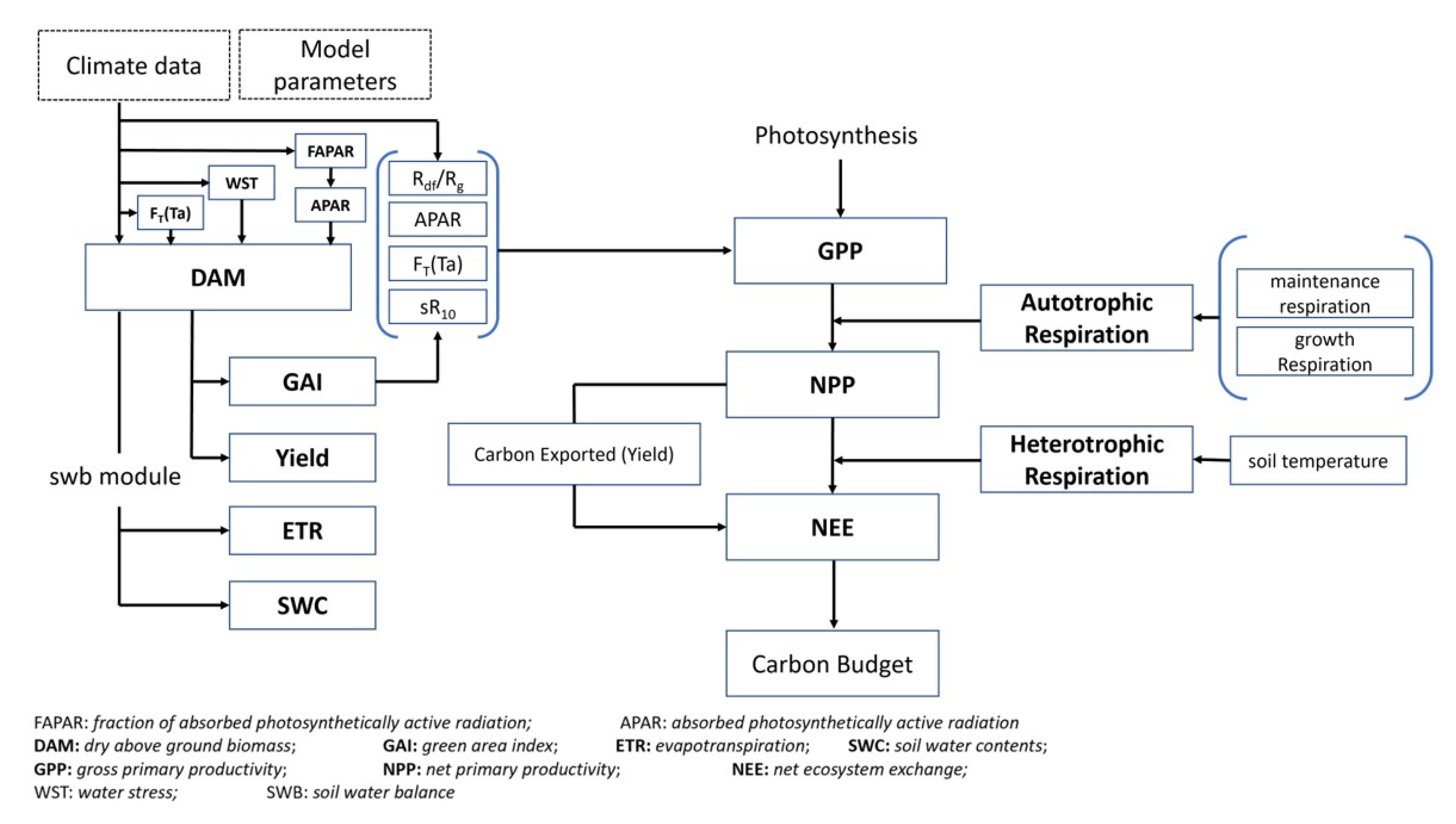
2.6. Model Overview
2.7. Model Evaluation
3. Results
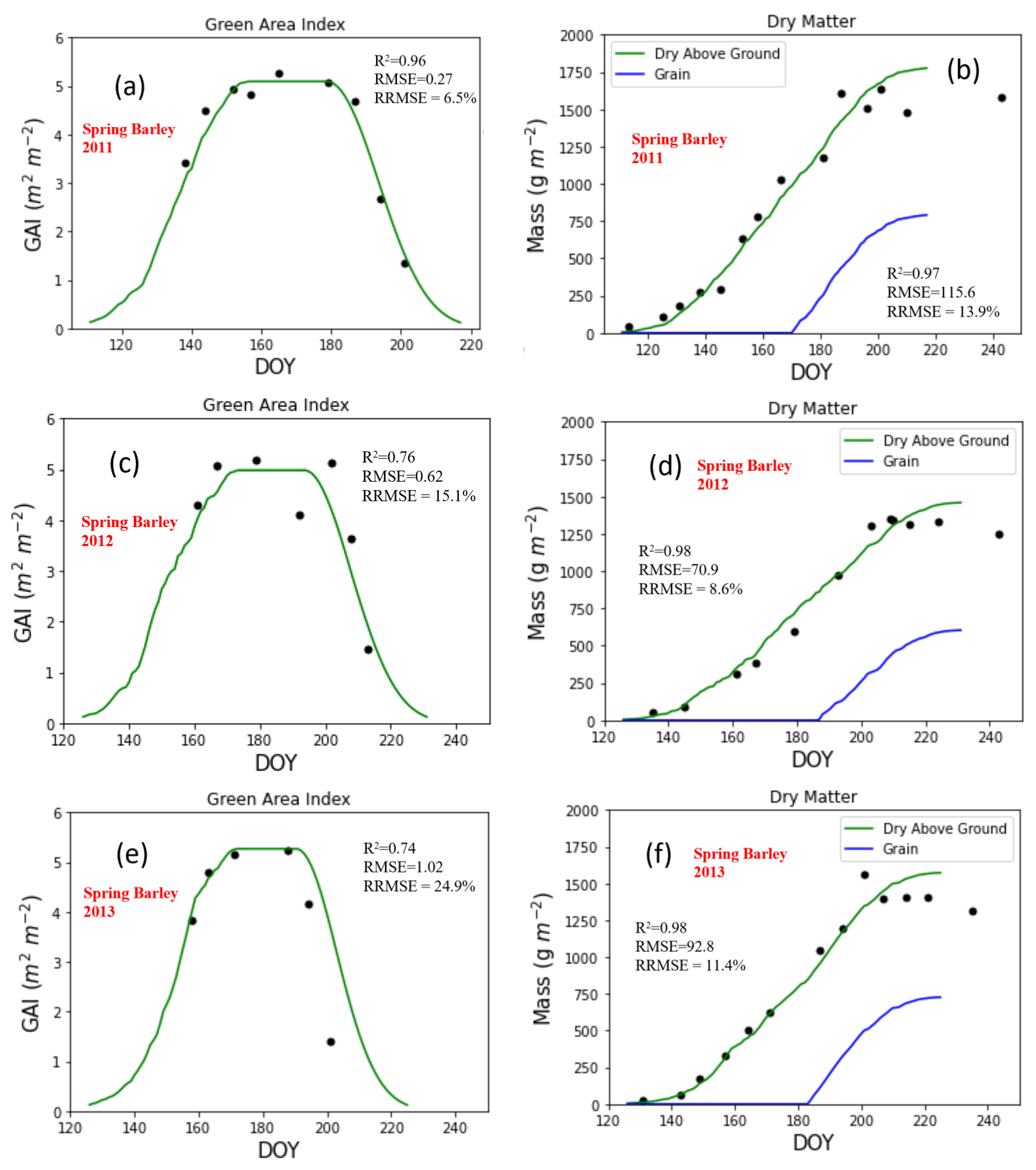
3.1. Sping Barley
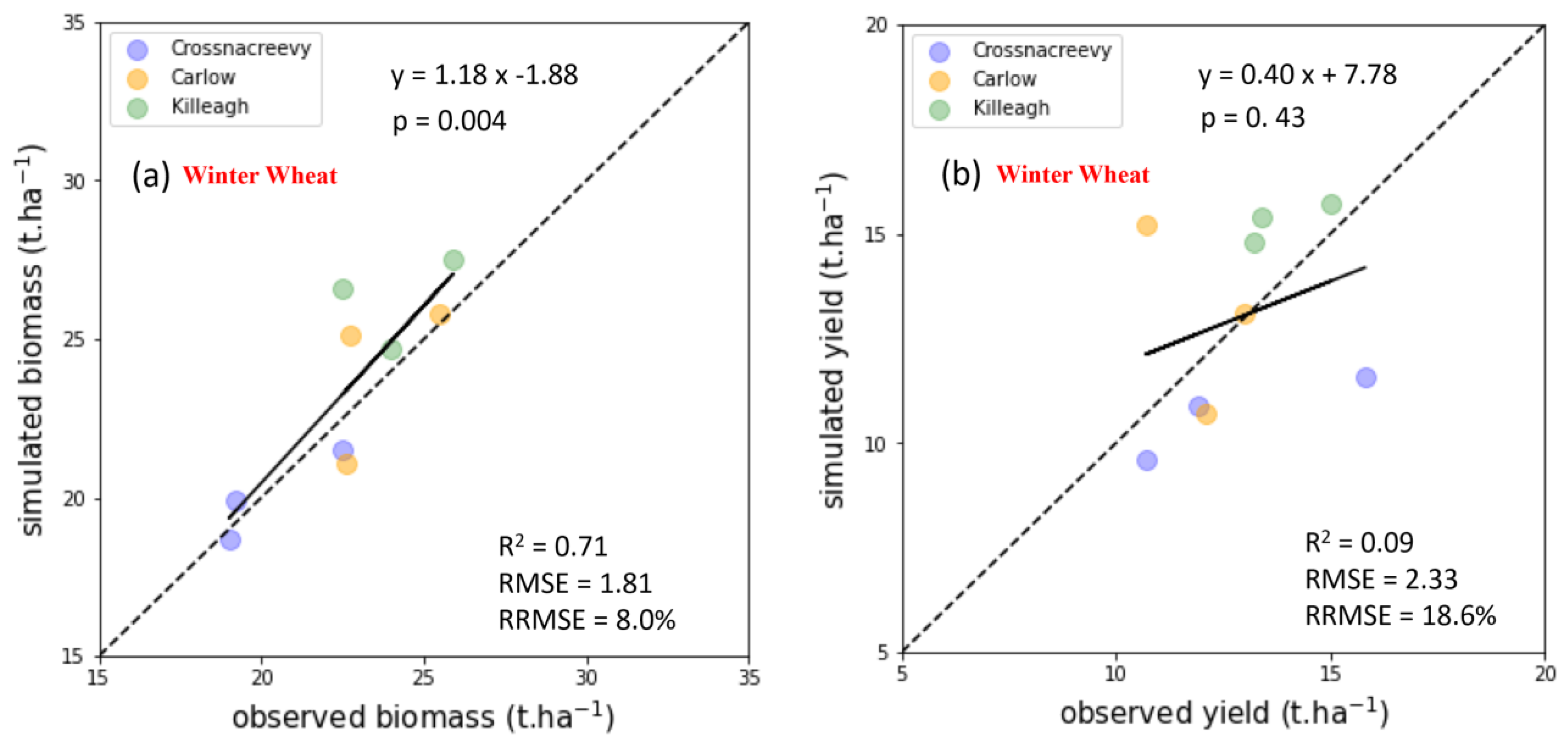
3.2. Winter Wheat
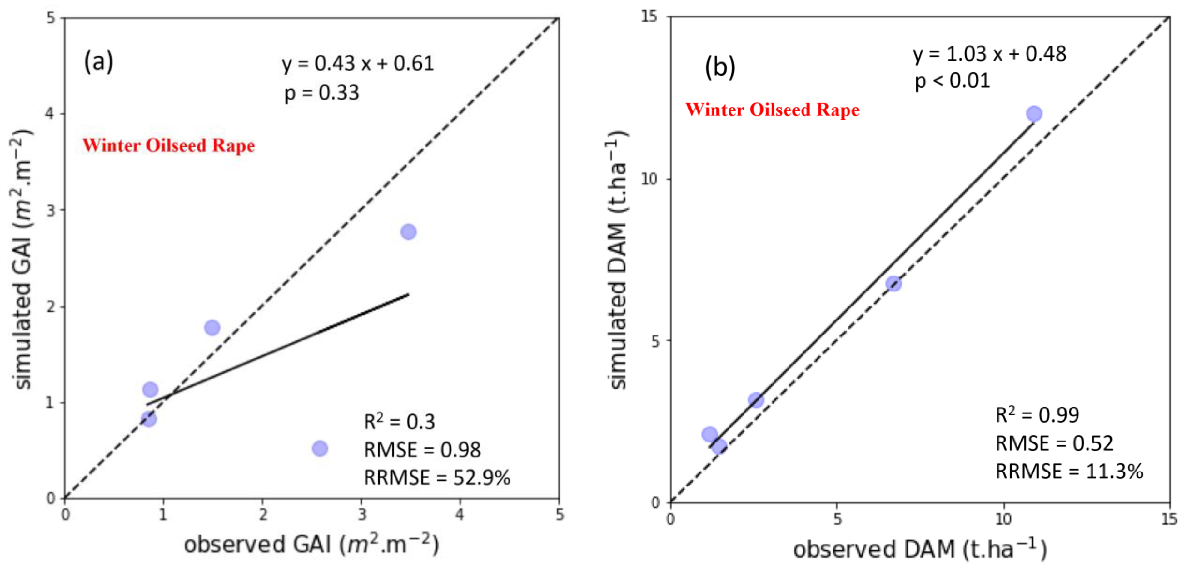
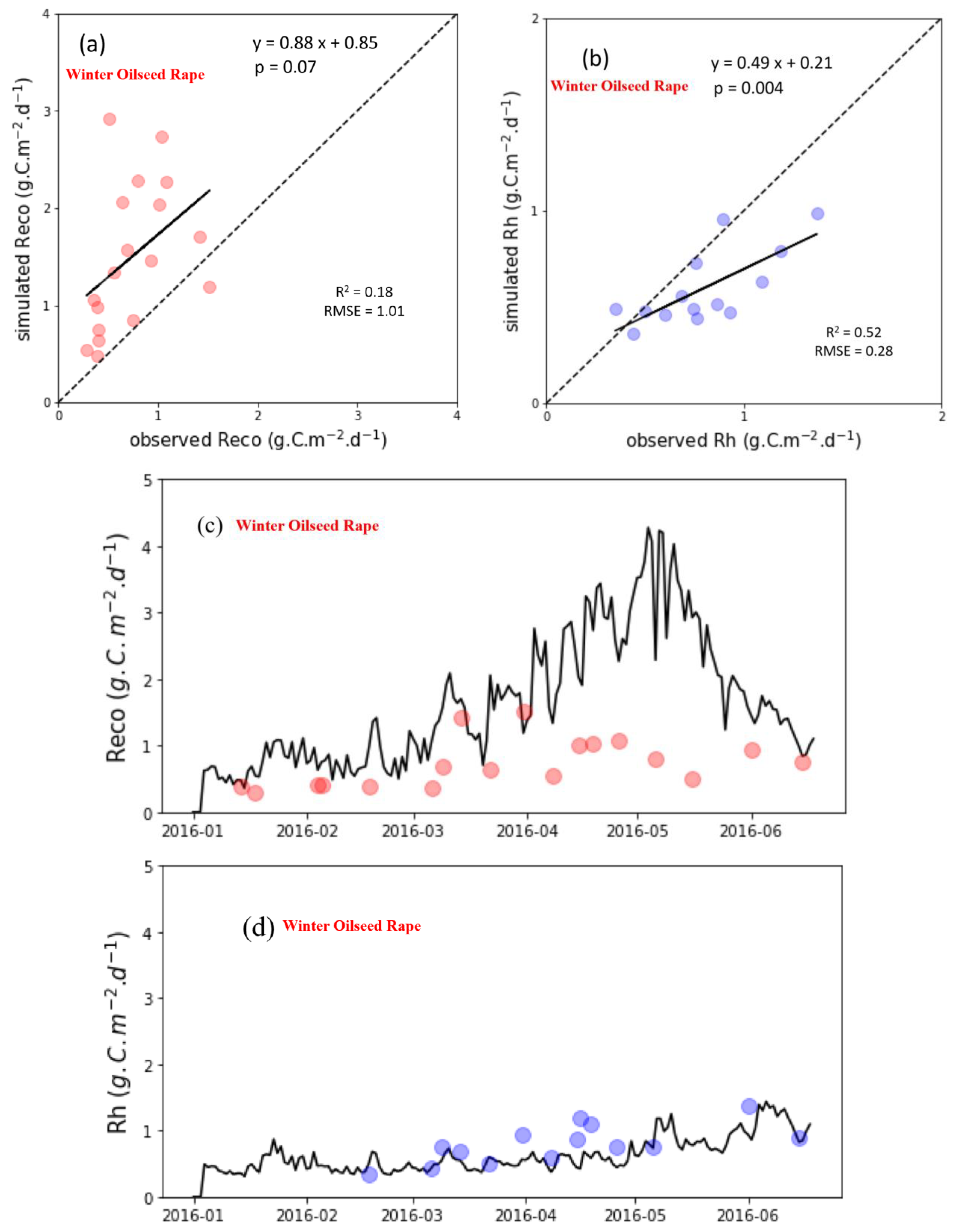
3.3. Winter Oilseed Rape
4. Discussion
4.1. Spring Barley (SB)
4.2. Winter Wheat (WW)
4.3. Winter Oil Seed Rape (WOSR)
5. Conclusions
Supplementary Materials
Author Contributions
Funding
Institutional Review Board Statement
Informed Consent Statement
Data Availability Statement
Acknowledgments
Conflicts of Interest
References
- Zimmermann, J.; Lydon, K.; Packham, I.; Smith, G.; Green, S. The Irish Land-Parcels Identification System (LPIS)–Experiences in Ongoing and Recent Environmental Research and Land Cover Mapping. R. Ir. Acad. 2016, 116, 53–62. [Google Scholar] [CrossRef]
- Spink, J.; Hennessy, M.; Lynch, J.; O’Donovan, T.; Forristal, D.; Hackett, R.; Kildea, S.; Glynn, L.; Hickey, C.; Kennedy, S.; et al. The Spring Barley Guide; Teagasc Agriculture and Food Development Authority: Carlow, Ireland, 2018; Available online: https://www.teagasc.ie/publications/2015/the-spring-barley-guide.php (accessed on 17 November 2022).
- Lynch, J.; Spink, J.; Doyle, D.; Hackett, R.; Phelan, S.; Forristal, D.; Kildea, S.; Glynn, L.; Plunkett, M.; Wall, D.; et al. The Winter Wheat Guide; Teagasc Agriculture and Food Development Authority: Carlow, Ireland, 2016; p. 40. Available online: https://www.teagasc.ie/publications/2016/the-winter-wheat-guide.php (accessed on 17 November 2022).
- Emmet-Booth, J.P.; Dekker, S.; O’Brien, P. Climate Change Mitigation and the Irish Agriculture and Land Use Sector; Working Paper on Climate Change Advisory Council: Dublin, Ireland, 2019. [Google Scholar]
- Ciais, P.; Gervois, S.; Vuichard, N.; Piao, S.; Viovy, N. Effects of Land Use Change and Management on the European Cropland Carbon Balance. Glob. Change Biol. 2011, 17, 320–338. [Google Scholar] [CrossRef]
- Brilli, L.; Bechini, L.; Bindi, M.; Carozzi, M.; Cavalli, D.; Conant, R.; Dorich, C.D.; Doro, L.; Ehrhardt, F.; Farina, R. Review and Analysis of Strengths and Weaknesses of Agro-Ecosystem Models for Simulating C and N Fluxes. Sci. Total Environ. 2017, 598, 445–470. [Google Scholar] [CrossRef] [PubMed]
- Huang, Y.; Yu, Y.; Zhang, W.; Sun, W.; Liu, S.; Jiang, J.; Wu, J.; Yu, W.; Wang, Y.; Yang, Z. Agro-C: A Biogeophysical Model for Simulating the Carbon Budget of Agroecosystems. Agric. For. Meteorol. 2009, 149, 106–129. [Google Scholar] [CrossRef]
- Wattenbach, M.; Sus, O.; Vuichard, N.; Lehuger, S.; Gottschalk, P.; Li, L.; Leip, A.; Williams, M.; Tomelleri, E.; Kutsch, W.L. The Carbon Balance of European Croplands: A Cross-Site Comparison of Simulation Models. Agric. Ecosyst. Environ. 2010, 139, 419–453. [Google Scholar] [CrossRef]
- Zhang, X.; Izaurralde, R.C.; Manowitz, D.H.; Sahajpal, R.; West, T.O.; Thomson, A.M.; Xu, M.; Zhao, K.; LeDuc, S.D.; Williams, J.R. Regional Scale Cropland Carbon Budgets: Evaluating a Geospatial Agricultural Modeling System Using Inventory Data. Environ. Model. Softw. 2015, 63, 199–216. [Google Scholar] [CrossRef]
- Rauff, K.O.; Bello, R. A Review of Crop Growth Simulation Models as Tools for Agricultural Meteorology. Agric. Sci. 2015, 6, 1098. [Google Scholar] [CrossRef]
- Xinyou, Y.; Van Laar, H. Crop Systems Dynamics: An Ecophysiological Simulation Model of Genotype-by-Environment Interactions; Wageningen Academic Publishers: Wageningen, The Netherlands, 2005; ISBN 90-76998-55-8. [Google Scholar]
- Van Laar, H.H. Simulation of Crop Growth for Potential and Water-Limited Production Situations: As Applied to Spring Wheat. 1992. Available online: https://library.wur.nl/WebQuery/wurpubs/fulltext/359573 (accessed on 17 November 2022).
- Duchemin, B.; Maisongrande, P.; Boulet, G.; Benhadj, I. A Simple Algorithm for Yield Estimates: Evaluation for Semi-Arid Irrigated Winter Wheat Monitored with Green Leaf Area Index. Environ. Model. Softw. 2008, 23, 876–892. [Google Scholar] [CrossRef]
- Duchemin, B.; Fieuzal, R.; Rivera, M.A.; Ezzahar, J.; Jarlan, L.; Rodriguez, J.C.; Hagolle, O.; Watts, C. Impact of Sowing Date on Yield and Water Use Efficiency of Wheat Analyzed through Spatial Modeling and FORMOSAT-2 Images. Remote Sens. 2015, 7, 5951–5979. [Google Scholar] [CrossRef]
- Brisson, N.; Gary, C.; Justes, E.; Roche, R.; Mary, B.; Ripoche, D.; Zimmer, D.; Sierra, J.; Bertuzzi, P.; Burger, P. An Overview of the Crop Model STICS. Eur. J. Agron. 2003, 18, 309–332. [Google Scholar] [CrossRef]
- Mackinnon, J.C. CERES-Maize: A Simulation Model of Maize Growth and Development: C.A. Jones and J.R. Kiniry (Editors). Texas A&M University Press, College Station, TX, 1986. 194 Pp., US$33.50. ISBN 0-89096-269-3. Comput. Electron. Agric. 1987, 2, 171–172. [Google Scholar] [CrossRef]
- Constantin, J.; Willaume, M.; Murgue, C.; Lacroix, B.; Therond, O. The Soil-Crop Models STICS and AqYield Predict Yield and Soil–water Content for Irrigated Crops Equally Well with Limited Data. Agric. For. Meteorol. 2015, 206, 55–68. [Google Scholar] [CrossRef]
- Steduto, P.; Hsiao, T.C.; Raes, D.; Fereres, E. AquaCrop—The FAO Crop Model to Simulate Yield Response to Water: I. Concepts and Underlying Principles. Agron. J. 2009, 101, 426–437. [Google Scholar] [CrossRef]
- Brunel-Muguet, S.; Mollier, A.; Kauffmann, F.; Avice, J.-C.; Goudier, D.; Sénécal, E.; Etienne, P. SuMoToRI, an Ecophysiological Model to Predict Growth and Sulfur Allocation and Partitioning in Oilseed Rape (Brassica napus L.) until the Onset of Pod Formation. Front. Plant Sci. 2015, 6, 993. [Google Scholar] [CrossRef] [PubMed]
- Habekotte, B. Evaluation of Seed Yield Determining Factors of Winter Oilseed Rape (Brassica napus L.) by Means of Crop Growth Modelling. Field Crops Res. 1997, 54, 137–151. [Google Scholar] [CrossRef]
- Upreti, D.; Pignatti, S.; Pascucci, S.; Tolomio, M.; Huang, W.; Casa, R. Bayesian Calibration of the Aquacrop-OS Model for Durum Wheat by Assimilation of Canopy Cover Retrieved from VENµS Satellite Data. Remote Sens. 2020, 12, 2666. [Google Scholar] [CrossRef]
- Upreti, D.; Pignatti, S.; Pascucci, S.; Tolomio, M.; Li, Z.; Huang, W.; Casa, R. A Comparison of Moment-Independent and Variance-Based Global Sensitivity Analysis Approaches for Wheat Yield Estimation with the Aquacrop-OS Model. Agronomy 2020, 10, 607. [Google Scholar] [CrossRef]
- Lynch, J.; Fealy, R.; Doyle, D.; Black, L.; Spink, J. Assessment of Water-Limited Winter Wheat Yield Potential at Spatially Contrasting Sites in Ireland Using a Simple Growth and Development Model. Ir. J. Agric. Food Res. 2017, 56, 65–76. [Google Scholar] [CrossRef]
- Kang, Y.; Özdoğan, M. Field-Level Crop Yield Mapping with Landsat Using a Hierarchical Data Assimilation Approach. Remote Sens. Environ. 2019, 228, 144–163. [Google Scholar] [CrossRef]
- Pique, G.; Fieuzal, R.; Debaeke, P.; Al Bitar, A.; Tallec, T.; Ceschia, E. Combining High-Resolution Remote Sensing Products with a Crop Model to Estimate Carbon and Water Budget Components: Application to Sunflower. Remote Sens. 2020, 12, 2967. [Google Scholar] [CrossRef]
- Shirley, R.; Pope, E.; Bartlett, M.; Oliver, S.; Quadrianto, N.; Hurley, P.; Duivenvoorden, S.; Rooney, P.; Barrett, A.B.; Kent, C. An Empirical, Bayesian Approach to Modelling Crop Yield: Maize in USA. Environ. Res. Commun. 2020, 2, 025002. [Google Scholar] [CrossRef]
- Claverie, M.; Demarez, V.; Duchemin, B.; Hagolle, O.; Ducrot, D.; Marais-Sicre, C.; Dejoux, J.-F.; Huc, M.; Keravec, P.; Béziat, P. Maize and Sunflower Biomass Estimation in Southwest France Using High Spatial and Temporal Resolution Remote Sensing Data. Remote Sens. Environ. 2012, 124, 844–857. [Google Scholar] [CrossRef]
- Silvestro, P.C.; Pignatti, S.; Yang, H.; Yang, G.; Pascucci, S.; Castaldi, F.; Casa, R. Sensitivity Analysis of the Aquacrop and SAFYE Crop Models for the Assessment of Water Limited Winter Wheat Yield in Regional Scale Applications. PLoS ONE 2017, 12, e0187485. [Google Scholar] [CrossRef] [PubMed]
- Silvestro, P.C.; Casa, R.; Hanuš, J.; Koetz, B.; Rascher, U.; Schuettemeyer, D.; Siegmann, B.; Skokovic, D.; Sobrino, J.; Tudoroiu, M. Synergistic Use of Multispectral Data and Crop Growth Modelling for Spatial and Temporal Evapotranspiration Estimations. Remote Sens. 2021, 13, 2138. [Google Scholar] [CrossRef]
- Silvestro, P.; Pignatti, S.; Pascucci, S.; Yang, H.; Li, Z.; Yang, G.; Huang, W.; Casa, R. Estimating Wheat Yield in China at the Field and District Scale from the Assimilation of Satellite Data into the Aquacrop and Simple Algorithm for Yield (SAFY) Models. Remote Sens. 2017, 9, 509. [Google Scholar] [CrossRef]
- Pignatti, S.; Casa, R.; Laneve, G.; Li, Z.; Liu, L.; Marzialetti, P.; Mzid, N.; Pascucci, S.; Silvestro, P.C.; Tolomio, M. Sino–EU Earth Observation Data to Support the Monitoring and Management of Agricultural Resources. Remote Sens. 2021, 13, 2889. [Google Scholar] [CrossRef]
- Pique, G.; Fieuzal, R.; Al Bitar, A.; Veloso, A.; Tallec, T.; Brut, A.; Ferlicoq, M.; Zawilski, B.; Dejoux, J.-F.; Gibrin, H. Estimation of Daily CO2 Fluxes and of the Components of the Carbon Budget for Winter Wheat by the Assimilation of Sentinel 2-like Remote Sensing Data into a Crop Model. Geoderma 2020, 376, 114428. [Google Scholar] [CrossRef]
- Casa, R.; Upreti, D.; Pelosi, F. Measurement and Estimation of Leaf Area Index (LAI) Using Commercial Instruments and Smartphone-Based Systems; IOP Publishing: Bristol, UK, 2019; Volume 275, p. 012006. [Google Scholar] [CrossRef]
- Upreti, D.; Huang, W.; Kong, W.; Pascucci, S.; Pignatti, S.; Zhou, X.; Ye, H.; Casa, R. A Comparison of Hybrid Machine Learning Algorithms for the Retrieval of Wheat Biophysical Variables from Sentinel-2. Remote Sens. 2019, 11, 481. [Google Scholar] [CrossRef]
- Casa, R.; Upreti, D.; Palombo, A.; Pascucci, S.; Yang, H.; Yang, G.; Huang, W.; Pignatti, S. Evaluation and Exploitation of Retrieval Algorithms for Estimating Biophysical Crop Variables Using Sentinel-2, Venus, and PRISMA Satellite Data. J. Geod. Geoinf. Sci. 2021, 3, 79–88. [Google Scholar]
- Peel, M.C.; Finlayson, B.L.; McMahon, T.A. Updated World Map of the Köppen-Geiger Climate Classification. Hydrol. Earth Syst. Sci. 2007, 11, 1633–1644. [Google Scholar] [CrossRef]
- Éireann, M. A Summary of Climate Averages for Ireland 1981–2010; Met Éireann, Glasnevin Hill: Dublin, Ireland, 2012. [Google Scholar]
- Irish Soil Information System. Available online: https://www.teagasc.ie/environment/soil/irish-soil-information-system/ (accessed on 17 November 2022).
- Kennedy, S. Identifying Constraints to Increasing Yield Potential of Spring Barley; The University of Edinburgh: Edinburgh, UK, 2015. [Google Scholar]
- O’Neill, M.; Lanigan, G.J.; Forristal, P.D.; Osborne, B.A. Greenhouse Gas Emissions and Crop Yields from Winter Oilseed Rape Cropping Systems Are Unaffected by Management Practices. Front. Environ. Sci. 2021, 9, 377. [Google Scholar] [CrossRef]
- Hengl, T.; Mendes de Jesus, J.; Heuvelink, G.B.; Ruiperez Gonzalez, M.; Kilibarda, M.; Blagotić, A.; Shangguan, W.; Wright, M.N.; Geng, X.; Bauer-Marschallinger, B. SoilGrids250m: Global Gridded Soil Information Based on Machine Learning. PLoS ONE 2017, 12, e0169748. [Google Scholar] [CrossRef] [PubMed]
- Poggio, L.; De Sousa, L.M.; Batjes, N.H.; Heuvelink, G.; Kempen, B.; Ribeiro, E.; Rossiter, D. SoilGrids 2.0: Producing Soil Information for the Globe with Quantified Spatial Uncertainty. Soil 2021, 7, 217–240. [Google Scholar] [CrossRef]
- Pollacco, J.A.P. A Generally Applicable Pedotransfer Function That Estimates Field Capacity and Permanent Wilting Point from Soil Texture and Bulk Density. Can. J. Soil Sci. 2008, 88, 761–774. [Google Scholar] [CrossRef]
- Santra, P.; Kumar, M.; Kumawat, R.; Painuli, D.; Hati, K.; Heuvelink, G.; Batjes, N. Pedotransfer Functions to Estimate Soil–water Content at Field Capacity and Permanent Wilting Point in Hot Arid Western India. J. Earth Syst. Sci. 2018, 127, 1–16. [Google Scholar] [CrossRef]
- Wu, X.; Lu, G.; Wu, Z.; He, H.; Zhou, J.; Liu, Z. An Integration Approach for Mapping Field Capacity of China Based on Multi-Source Soil Datasets. Water 2018, 10, 728. [Google Scholar] [CrossRef]
- Monteith, J.L. Climate and the Efficiency of Crop Production in Britain. Philos. Trans. R. Soc. Lond. B Biol. Sci. 1977, 281, 277–294. [Google Scholar] [CrossRef]
- Wallach, D.; Makowski, D.; Jones, J.W.; Brun, F. Working with Dynamic Crop Models: Methods, Tools and Examples for Agriculture and Environment; Academic Press: Cambridge, MA, USA, 2018; ISBN 0-12-811757-5. [Google Scholar]
- De Jong, R.; Shaykewich, C.; Reimer, A. The Net Radiation Flux and Its Prediction at Pinawa, Manitoba. Argic. Meteorol. 1980, 22, 217–225. [Google Scholar] [CrossRef]
- McCree, K. Equations for the Rate of Dark Respiration of White Clover and Grain Sorghum, as Functions of Dry Weight, Photosynthetic Rate, and Temperature 1. Crop Sci. 1974, 14, 509–514. [Google Scholar] [CrossRef]
- Chahbi Bellakanji, A.; Zribi, M.; Lili-Chabaane, Z.; Mougenot, B. Forecasting of Cereal Yields in a Semi-Arid Area Using the Simple Algorithm for Yield Estimation (SAFY) Agro-Meteorological Model Combined with Optical SPOT/HRV Images. Sensors 2018, 18, 2138. [Google Scholar] [CrossRef]
- Bendig, J.; Bolten, A.; Bennertz, S.; Broscheit, J.; Eichfuss, S.; Bareth, G. Estimating Biomass of Barley Using Crop Surface Models (CSMs) Derived from UAV-Based RGB Imaging. Remote Sens. 2014, 6, 10395–10412. [Google Scholar] [CrossRef]
- Fletcher, A.; Martin, R.; de Ruiter, J.; Jamieson, P.; Zyskowski, R. Simulating Biomass and Grain Yields of Barley and Oat Crops with the Sirius Wheat Model. In Crop Modeling and Decision Support; Springer: Berlin/Heidelberg, Germany, 2009; pp. 192–202. [Google Scholar] [CrossRef]
- Rötter, R.P.; Palosuo, T.; Kersebaum, K.C.; Angulo, C.; Bindi, M.; Ewert, F.; Ferrise, R.; Hlavinka, P.; Moriondo, M.; Nendel, C. Simulation of Spring Barley Yield in Different Climatic Zones of Northern and Central Europe: A Comparison of Nine Crop Models. Field Crops Res. 2012, 133, 23–36. [Google Scholar] [CrossRef]
- Wengert, M.; Piepho, H.-P.; Astor, T.; Graß, R.; Wijesingha, J.; Wachendorf, M. Assessing Spatial Variability of Barley Whole Crop Biomass Yield and Leaf Area Index in Silvoarable Agroforestry Systems Using UAV-Borne Remote Sensing. Remote Sens. 2021, 13, 2751. [Google Scholar] [CrossRef]
- Khan, A.; Stöckle, C.O.; Nelson, R.L.; Peters, T.; Adam, J.C.; Lamb, B.; Chi, J.; Waldo, S. Estimating Biomass and Yield Using Metric Evapotranspiration and Simple Growth Algorithms. Agron. J. 2019, 111, 536–544. [Google Scholar] [CrossRef]
- Allies, A.; Roumiguié, A.; Fieuzal, R.; Dejoux, J.-F.; Jacquin, A.; Veloso, A.; Champolivier, L.; Baup, F. Assimilation of Multisensor Optical and Multiorbital SAR Satellite Data in a Simplified Agrometeorological Model for Rapeseed Crops Monitoring. IEEE J. Sel. Top. Appl. Earth Obs. Remote Sens. 2021, 15, 1123–1138. [Google Scholar] [CrossRef]
- Hussain, S.; Gao, K.; Din, M.; Gao, Y.; Shi, Z.; Wang, S. Assessment of UAV-Onboard Multispectral Sensor for Non-Destructive Site-Specific Rapeseed Crop Phenotype Variable at Different Phenological Stages and Resolutions. Remote Sens. 2020, 12, 397. [Google Scholar] [CrossRef]
- Lehuger, S.; Gabrielle, B.; Cellier, P.; Loubet, B.; Roche, R.; Béziat, P.; Ceschia, E.; Wattenbach, M. Predicting the Net Carbon Exchanges of Crop Rotations in Europe with an Agro-Ecosystem Model. Agric. Ecosyst. Environ. 2010, 139, 384–395. [Google Scholar] [CrossRef]


| Crop-Year | Sowing | Emergence | Senescence | Harvest | Crop Site | Nearest Weather Station |
|---|---|---|---|---|---|---|
| SB-2011 | March | April | August | August–September | DN | JC |
| SB-2012 | April | April | August | August–September | DN | JC |
| SB-2013 | April | April | August | August–September | DN | JC |
| WW-2013 | October–November | January–February | June | July–September | CR, CC, KL | AG, OP, RP |
| WW-2014 | October | January–February | June | July–September | CR, CC, KL | AG, OP, RP |
| WW-2015 | November–December | January–February | June | July–September | CR, CC, KL | AG, OP, RP |
| WOSR-2015 | September | January | June–July | August | GN | OP |
| Site | Year | Recorded | Observed | Simulated | ||||
|---|---|---|---|---|---|---|---|---|
| Sowing Date | Y (t/ha) | B (t/ha) | GS 61 | Y (t/ha) | B (t/ha) | GS 61 | ||
| Crossnacreevy | 2013 | 8-November | 15.8 | 19.2 | 25-June | 11.6 | 19.9 | 14-June |
| 2014 | 29-October | 10.7 | 19 | 16-June | 9.6 | 18.7 | 9-June | |
| 2015 | 4-December | 11.9 | 22.5 | 30-June | 10.9 | 21.5 | 28-June | |
| Carlow | 2013 | 25-October | 10.7 | 18 | 19-June | 15.2 | 25.8 | 7-June |
| 2014 | 14-October | 12.1 | 25.5 | 11-June | 10.7 | 21.1 | 21-June | |
| 2015 | 14-October | 13 | 22.6 | 13-June | 13.1 | 25.1 | 12-June | |
| Killeagh | 2013 | 23-October | 15 | 22.5 | 18-June | 15.7 | 26.6 | 31-May |
| 2014 | 15-October | 13.4 | 25.9 | 10-June | 15.4 | 27.5 | 8-June | |
| 2015 | 6-November | 13.2 | 24 | 14-June | 14.8 | 24.7 | 4-June | |
Publisher’s Note: MDPI stays neutral with regard to jurisdictional claims in published maps and institutional affiliations. |
© 2022 by the authors. Licensee MDPI, Basel, Switzerland. This article is an open access article distributed under the terms and conditions of the Creative Commons Attribution (CC BY) license (https://creativecommons.org/licenses/by/4.0/).
Share and Cite
Upreti, D.; McCarthy, T.; O’Neill, M.; Ishola, K.; Fealy, R. Application and Evaluation of a Simple Crop Modelling Framework: A Case Study for Spring Barley, Winter Wheat and Winter Oilseed Rape over Ireland. Agronomy 2022, 12, 2900. https://doi.org/10.3390/agronomy12112900
Upreti D, McCarthy T, O’Neill M, Ishola K, Fealy R. Application and Evaluation of a Simple Crop Modelling Framework: A Case Study for Spring Barley, Winter Wheat and Winter Oilseed Rape over Ireland. Agronomy. 2022; 12(11):2900. https://doi.org/10.3390/agronomy12112900
Chicago/Turabian StyleUpreti, Deepak, Tim McCarthy, Macdara O’Neill, Kazeem Ishola, and Rowan Fealy. 2022. "Application and Evaluation of a Simple Crop Modelling Framework: A Case Study for Spring Barley, Winter Wheat and Winter Oilseed Rape over Ireland" Agronomy 12, no. 11: 2900. https://doi.org/10.3390/agronomy12112900
APA StyleUpreti, D., McCarthy, T., O’Neill, M., Ishola, K., & Fealy, R. (2022). Application and Evaluation of a Simple Crop Modelling Framework: A Case Study for Spring Barley, Winter Wheat and Winter Oilseed Rape over Ireland. Agronomy, 12(11), 2900. https://doi.org/10.3390/agronomy12112900