UAV Multispectral Imaging Potential to Monitor and Predict Agronomic Characteristics of Different Forage Associations

Abstract

The capability of UAVs imagery to monitor and predict the evolution of several forage associations was assessed during the whole growing cycle of 2019–20. For this purpose, eight different forage associations grown in triplicate were used: vetch-barley-triticale (VBT), vetch-triticale (VT), vetch-rye (VR), vetch-oats (VO), pea-barley-triticale (PBT), pea-triticale (PT), pea-rye (PR) and pea-oats (PO). Six biophysical parameters were monitored through six vegetation indices on seven measurements dates distributed along the growing cycle. The experiments were carried out on the organic farm “Gallegos de Crespes” located in the municipality of Larrodrigo (Salamanca, Spain). The results obtained in the exploratory and the correlation analysis suggested that a predictive model (PLS regression) could be performed. Overall, vetch-based associations showed slightly higher values for both the field parameters and the vegetation indices than pea-based ones. Correlations were very strong and significant for each association throughout their growing cycle, suggesting that the evolution of the associations would be monitored from the spectral indices. Integrating these multispectral observations in the PLS model, the agronomic parameters of forage associations were predicted with a reliability of more than 50%. A single combination of VNIR (or even only visible) bands was able to feed the regression model, leading to a successful prediction of the agronomic parameters.

1. Introduction

Forages are one of the main feed sources for livestock, especially for ruminants, which are able to transform protein-poor feed into high-protein human consumption products such as meat and milk [1]. Generally, such forages are based exclusively on cereals such as barley, oats or wheat, among others, due to the high dry matter yield they produce at very low cost. These cereal-based forages provide large amounts of energy to the animals, but lack other vital elements such as protein, thus reducing their nutritional quality [2]. The separate purchase of protein supplements results in high feed cost, and considering that high quality forage optimizes animal productivity, increasing the quality of such forages is a much more effective method of improving overall feed efficiency [3]. One of the most cost-effective ways of increasing forage quality is by mixing cereal crops with others species capable of increasing the protein content of the overall ration, such as legumes. Crop associations or intercropping systems are defined as the simultaneous growing of two or more species on the same area during a significant period of their growing season [4]. These crop mixtures show several potential advantages over sole crops, as they have higher yields and greater yield’s stability from season to season, are more resistant to pests and diseases, improve forage production quality, maintain soil fertility due to legume’s biological fixation of nitrogen and increase microbiota biodiversity [5].

Considering the importance of forages in agriculture, it is necessary to carry out periodical assessments of the nutritional, physiological and sanitary status of forages throughout their growing cycle. This will allow to characterize the different crop associations and aid in estimating both the quality and potential yields of these crops [6]. Nowadays, the limited available methodologies to carry out this monitoring consist of painstaking field works (Hollinger 1997) usually divided into two stages. The first one is a non-invasive stage based on visual observations to check the phenological and sanitary state of the crop [7] and on parameter measurements that do not involve sample extraction, such as chlorophyll level [8], crop height or fractional vegetation cover (FVC) estimation [9], among others. On the other hand, the second stage is an invasive one and consists of collecting a sample over a known surface area in order to estimate leaf area index (LAI) [10], productive yield and forage quality [11,12].

Remote sensing, particularly piloted aircraft and satellite imagery (RGB, multispectral or hyperspectral), has emerged in the last twenty years as a widespread non-invasive methodology for crop monitoring [13]. However, their images lack high enough spatial resolution to perform accurate time series analysis [14]. In this context, drones or Unmanned Aerial Vehicles (UAVs) and the miniaturized sensors they carry have emerged as a useful technology. These sensors offer very high-resolution images, low operational and maintenance costs and instantaneous data transmission [15]. Among them, multispectral (MS) sensors stand out as one of the best options for assessing crop growth, biomass quantity and several biochemical indicators [16,17,18], specifically from forages [19]. The more common MS sensors are able to register five or six bands in the visible-near infrared spectra region. Using different algebraic combinations of these bands, a wide range of vegetation indices can be calculated. The most widespread due to its great versatility is the Normalized Difference Vegetation Index (NDVI) [20] as it not only provides information on the quality and development of vegetation, but has also been used to estimate productive yields in certain crops [21,22,23].

The hypothesis of the work is that it is possible, on the basis of a range of vegetation indices taken along the growing cycle, to predict several agronomic characteristics of crops at any moment of their growth cycle. If so, these indices could replace the laborious field work that must be carried out for in situ crop monitoring. Since the single indices may be insufficient to model the crop evolution, a wide range of regression models emerge as a way of integrate the information of all of them, such as the Support Vector Machine (SVM) [24], based on the machine learning theory, or the regression model based on Partial Least Squares (PLS) [25,26], which is a multivariate statistical tool with applications in many academic disciplines, including precision agriculture [27,28,29,30]. PLS is the most successful multivariate calibration method in the application of the combination of chemometrics with spectral data [31]. This technique addresses the problem of finding a linear regression model by mapping the explanatory variables and the observed variables into a new space. Besides, it is an easy and intuitive method that analyzes associations between two sets of data and highly recommended when the explanatory variables are correlated. It is a non-parametric technique which makes no distributional assumptions that works with small sample sizes [32]. The PLS transformations of the explanatory variables try to explain the covariance between the explanatory and observed variables as far as possible [33].

Considering the above, the present work shows a first screening of the potential of airborne multispectral images captured with UAVs for the monitoring and prediction of several in situ agronomic parameters of different forage associations. The research explored the relationships between a few spectral indices UAV-based and simultaneous field measurements over several fields of forage associations during a 2019–20 campaign. The indices suitability was first assessed after a descriptive analysis and a correlation analysis, whose promising results suggested the suitability of a robust mathematical method (PLS) to build a prediction model of the growing cycle parameters. Other contribution to the UAVs community is the assessment of the use of indices on the visible spectra as an alternative of the more costly infrared-based cameras. The paper was organized as follows: Section 2 explains the experimental layout, the data acquisition and the statistical analysis. Section 3 is devoted to the results and their discussion, and the Conclusions close the text.

2. Materials and Methods

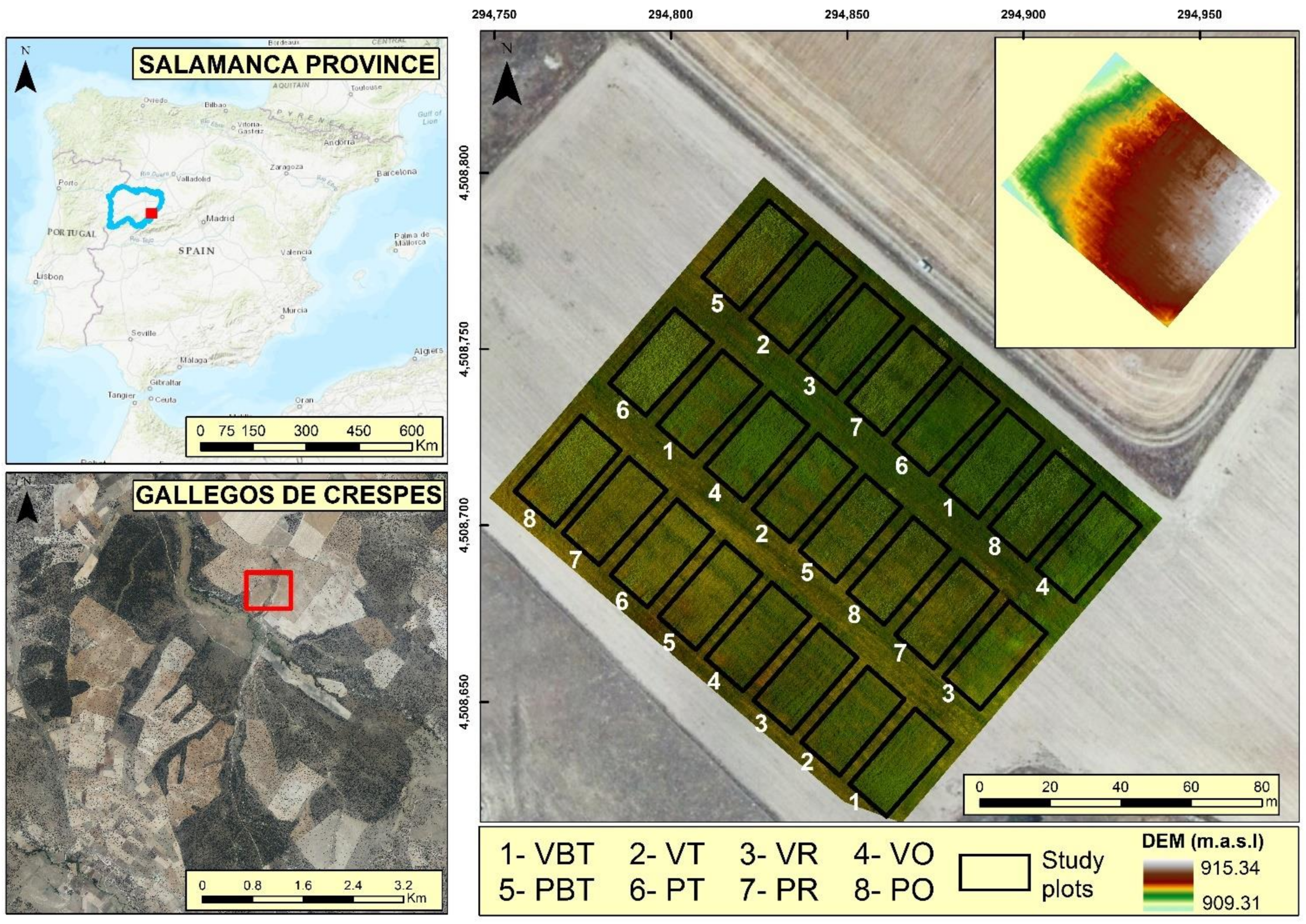
2.1. Experimental Design

This study was carried out from October 2019 to June 2020 on the organic production farm “Gallegos de Crespes” (40°42′13″ N–5°25′43″ W; 906 m a.s.l.) located in the municipality of Larrodrigo, in the southeast of the province of Salamanca in Castilla y León, Spain (Figure 1).

The climate in the area is Mediterranean with continental influence, characterized by a high thermal range and a frost period from October to April. According to the Spanish Meteorological Agency (AEMET), during the study period an average temperature of 9.50 °C, an accumulated rainfall of 380.34 mm and an accumulated radiation of 3893.05 MJ/m² were recorded. The crops were grown on a plain terrain on sandy, gravelly and pebbly soils over arcosic sandstones (pH 5.5–6 and sandy-clay-loam texture).

Six different forage crops were selected to form the subsequent crop mixtures: vetch (Vicia sativa cv. “Rada”), pea (Pisum sativum cv. “Cabestrón”), triticale (Triticum × Secale cv. “Elleac”), six-row barley (Hordeum vulgare ssp. Hexastichum cv. “Yuriko”), rye (Secale cereale cv. “Serafín”) and oat (Avena sativa cv. RGT “Chapela”). These crops were combined in eight different forage associations: vetch-barley-triticale (VBT), vetch-triticale (VT), vetch-rye (VR), vetch-oats (VO), pea-barley-triticale (PBT), pea-triticale (PT), pea-rye (PR) and pea-oats (PO). The associations containing vetch were sown at a rate of 140 kg/ha (70% legume—30% cereal) while those containing pea were sown at 130 kg/ha (60% legume—40% cereal). The sowing took place on 19 October 2019 and the harvesting on 10 June 2020. All the associations have a similar growing cycle under a rainfed regime.

Each association was grown in triplicate in a random block design of 24 experimental plots of 400 m² each, covering an area of approximately one hectare (Figure 1). The characterization of these associations was carried out over the first row of plots, numbered from 1 to 8 consecutively.

2.2. Field and Laboratory Estimations

Several biophysical parameters of the associations were monitored along the growing cycle of 2020 (n = 7 measurements on dates 02/04; 02/26; 03/26; 04/14; 05/02; 05/17; 05/29). To estimate them, both destructive (sample collection) and non-destructive methods were carried out in the field. Then, laboratory estimations were conducted to obtain final values. The following parameters were estimated at association level: the Leaf Area Index (LAI), the fresh and dry biomass (FB and DB), the vegetation water content (VWC) and the percentage of water content (PWC). On the other hand, using non-destructive field methods, the fraction of vegetation cover (FVC) was estimated. Other parameters were also estimated (e.g., plant height, chlorophyll) but were discarded here as they were collected at plant level.

Table 1. List of the field and laboratory parameters used in the study.

Field/Laboratory Parameters		Units
Fraction of Vegetation Cover	FVC	%
Leaf Area Index	LAI	m2/m2
Fresh biomass	FB	gr/m2
Dry biomass	DB	gr/m2
Vegetation Water Content	VWC	gr/m2
Percentage of Water Content	PWC	%

listed the selected parameters, which aimed to describe both the state of the plant and their rate of activity [34], and have been largely used in remote sensing applications to agronomy [35,36,37].

Two replicates of plant samples were taken at association level over a circular fenced area of 0.125 m², together with zenithal photographs taken at a same height of 1.5 m, following the protocol of Sánchez et al. [38]. Each sample was geolocated with a GPS receiver. Regarding the laboratory estimates, dry and wet weights of the sample were obtained, given that the wet weight is assumed as the FB, and their difference as the VWC expressed both in g/m² and in percentage. Forage samples were dried in a forced air oven at 60 °C for 48 h, until constant weight. To obtain the green LAI, leaf samples were scanned and digitally processed in the Image J software [39], which is a very common way to estimate the foliar area [40,41,42]. Finally, the FVC was estimated from the zenithal photographs using a supervised classification performed in PCI Geomatics Banff software, which allowed the segmentation of green/dry covers, bare soil and shadows [43].

2.3. Multispectral Imaging Collection and Vegetation Indices

Seven drone missions were flown simultaneously to the field measurements (around midday to avoid shadows). The mission area was approximately one hectare wide, and the flying altitude was fixed to 43 m above the ground. The UAV model was a DJI (SZ DJI Technology Co., Ltd., Shenzhen, China) Inspire1, with a Micasense (AgEagle Sensor Systems Inc., d/b/a MicaSense, Wichita, KS, USA) Red Edge M camera on board. The camera was mounted in the aircraft together with the GPS receiver and the downwelling light sensor using an ad hoc structure (Figure 2). The equipment was completed with a calibrated reflectance panel to radiometrically calibrate the imagery and four permanent ground control points to georeference the images.

The Micasense sensor is a multispectral camera with five discrete bands in the visible-near infrared spectra, namely blue (475 ± 20 nm), green (560 ± 20 nm), red (668 ± 10 nm), near infrared (840 ± 40 nm) and red edge (717 ± 10 nm). The imager resolution is 1280 × 960 pixels, that afforded a spatial resolution for the resulting maps of 3 cm for all the acquisitions. The treatment of images was performed in Pix4D Mapper (Pix4D P.A., Prilly, Switzerland) software using a customized template that included, in addition to the geometric corrections and orthomosaicking, the radiometric calibration and the retrieval of the corrected reflectance maps together with the vegetation indices.

Three indices were proposed, in the first place the aforementioned NDVI, the forefront of vegetation indices. Also, the normalized ratio between red and green bands, the Green-Red Vegetation Index (GRVI) [44], and the proportion of green reflectance in the whole RGB space, the so-called Greenness index. A red-edge version of the three was also obtained, replacing the red band for the red-edge one.

Table 2. Vegetation indices used in this study. $R_{NIR}$, $R_{redge}$, $R_{red}$, $R_{green}$ and $R_{blue}$ are the reflectance in the respective bands.

Vegetation Indices		Equation
Greenness	Gr	$\frac{R_{green}}{R_{red} + R_{green} + R_{blue}}$
Greenness_Red_Edge	Gr_redge	$\frac{R_{green}}{R_{redge} + R_{green} + R_{blue}}$
Normalized Difference Vegetation Index	NDVI	$\frac{R_{NIR} - R_{red}}{R_{NIR} + R_{red}}$
Normalized Difference Vegetation Index_Red_Edge	NDVI_redge	$\frac{R_{NIR} - R_{redge}}{R_{NIR} + R_{redge}}$
Green-Red Vegetation Index	GRVI	$\frac{R_{green} - R_{red}}{R_{green} + R_{red}}$
Green-Red Vegetation Index_Red_Edge	GRVI_redge	$\frac{R_{green} - R_{redge}}{R_{green} + R_{redge}}$

summarizes the six resulting vegetation indices and their formulation.

GRVI and Greenness were selected to investigate the feasibility of visible bands of RGB cameras, typically on board the UAVs, as an alternative to the most expensive multispectral cameras. RGB-based indices have been widely used to monitor vegetation status [45,46], particularly after the advent of UAVs applications in agronomy [47,48,49,50,51]. In this vein, GRVI was successfully applied to estimate biomass and yield [49,50,52], nitrogen [53] or phenology [54]. Besides, the Greenness index is a simple way to indicate the proportion of vegetation cover [45], so it is expected to be related with FVC and LAI.

An area similar in size to that of the field measurements was extracted over the indices at their locations, to be fairly compared with the vegetation estimations.

2.4. Statistical Analysis

2.4.1. Exploratory Analysis of Data Variability

In the first place, a comparative analysis at association level between the temporal evolution both of the field estimations and the indices was performed to examine their matching. Conversely, a comparison at each date of measurement was carried out to explore similarities in the behavior of the height associations and possible spatial patterns.

2.4.2. Correlation Analysis

In order to assess the relationships between field and remote variables, a bivariate correlation process was conducted using Pearson’s linear correlation coefficient [55] as correlation indicator. Two-tailed significance test was performed, flagging significant ($p\le {0.05}^{*}$) and highly significant ($p\le {0.01}^{**}$) correlations. As in the exploratory analysis, correlations (n = 16) for each association along time and correlations (n = 14) for each date at spatial basis were calculated. The former were obtained to prove the potential of multispectral images captured by drone-borne sensors to match the evolution of vegetation indices with the real evolution of the associations throughout their cycle. Conversely, the latter were calculated to test how well the spatial variability of the studied parameters at each association and location is captured by these vegetation indices. In addition, the spatial analysis makes it possible to investigate whether the performance and evolution of the crop depends on the association itself or on its spatial location, which could be useful for decision making on crop management by the farmer and is one of the premises of the precision agriculture. The results obtained in this correlation analysis may suggest (or not) a step forward in the application of the indices by integrating them in a predictive model.

2.4.3. Prediction Model of In Situ Agronomic Parameters along the Growing Cycle Based on Partial Least Squares (PLS) Regression

As previously mentioned, the aim of this work is to monitor and predict the set of field-measured variables (matrix $Y$), which play the role of dependent, observed or explained variables, through the vegetation indices obtained by the drone (matrix $X$), which would act as explanatory variables. To this end, after the exploratory and correlation analysis, a PLS regression model with the following algorithm was proposed:

Step 1. It considers the $X$ and $Y$ matrices given by the explanatory and standardized response variables, respectively.

Step 2. It computes a linear combination of the columns of $X$ and $Y$, denoted by $t_1$ and $u_1$, respectively, in order to maximize the covariance, cov ($t_1$, $u_1$).

Step 3. It computes a classical linear regression model for the explanatory and response variables based on the value of the component $t_1$, given by:

$$X=t_1{p}_1^t+X_1\mathrm{and}Y=t_1{r}_1^t+Y_1$$

where $p_1$ and $r_1$ are the regression coefficients.

Step 4. It repeats the first step by substituting $X$ and $Y$ by the residual matrices $X_1$ e $Y_1$. Analogously, we obtain two new components $t_2$ and $u_2$, as linear combinations of the columns of $X_1$ and $Y_1$, respectively, which maximize the covariance, cov ($t_2$, $u_2$). It computes again a linear regression model:

$$X_1=t_2{p}_2^t+X_2\mathrm{and}{Y}_1=t_2{r}_2^t+Y_2$$

where $X$ and $Y$ can be expressed recursively by the components $t_1$ and $t_2$,

$$X=t_1{p}_1^t+t_2{p}_2^t+X_2\mathrm{and}Y=t_1{r}_1^t+t_2{r}_2^t+Y_2$$

where $X$ and $Y$ can be expressed recursively by the components $t_1$ and $t_2$,

$$X=t_1{p}_1^t+t_2{p}_2^t+X_2\mathrm{and}Y=t_1{r}_1^t+t_2{r}_2^t+Y_2$$

Step 5. It repeats this process until no significant improvement is seen in the explanation of $Y$. The algorithm ensures orthogonal components—uncorrelated—which are linear combinations of $X$.

Step 6. From the expression of $Y$ as a function of the selected $h$ components, $t_1,\dots ,t_{\mathrm{h}}$ it can be easily computed the PLS regression equations of any response variable based on the explanatory variables.

The criteria of selecting the number of components, $h$, is based in the so-called Leave-One-Out Cross Validation (LOOCV) scheme. A single sample is deleted from the calibration set, developing a model with the remaining ones and predicting for the single left-out sample. The process is repeated as many times as samples and the squared prediction errors are summed up. This leads to the computation of the Predicted Residual Sum of Squares (PRESS) for the $k{t}_{\mathrm{h}}$ response variable as a function of model dimensionality, PRESS ($k$,$h$). Based on PRESS ($k$,$h$) the predicted R-squared is computed, $R^2\left(k,h\right)$. Finally, the mean predicted R-squared, $R^2 \left(h\right)$, is computed as the average of $R^2\left(k,h\right)$ for all response variables. Also PRESS $\left(h\right)$ can be computed as the sum of PRESS $\left(k,h\right)$. In this model, a $R^2 \left(h\right)$ plot is used to draw conclusions. The best number of components is the one that maximize the overall mean predicted R-squared. Using the parsimony principle, if the $R^2 \left(h\right)$ plot does not exhibit abrupt changes it will be chosen the model having a fewer number of parameters.

Although all the crop associations are compositionally different, the fact that all of them are formed by leguminous species in combination with winter cereal species means that they all have very similar behaviors throughout their growth cycles. On this premise, from an analytical point of view, it seems more suitable to consider the eight associations as a whole sample of the same population (n = 112), rather than treating them individually (n = 14). Advantages of this consideration imply a simplification in the understanding of the results and a better predictive capacity of the PLS regression model. This assumption was assessed by the results drawn from the exploratory analysis.

All the statistical processing was conducted using IBM-SPSS Statistics 26 software (IBM, Chicago, IL, USA).

3. Results and Discussion

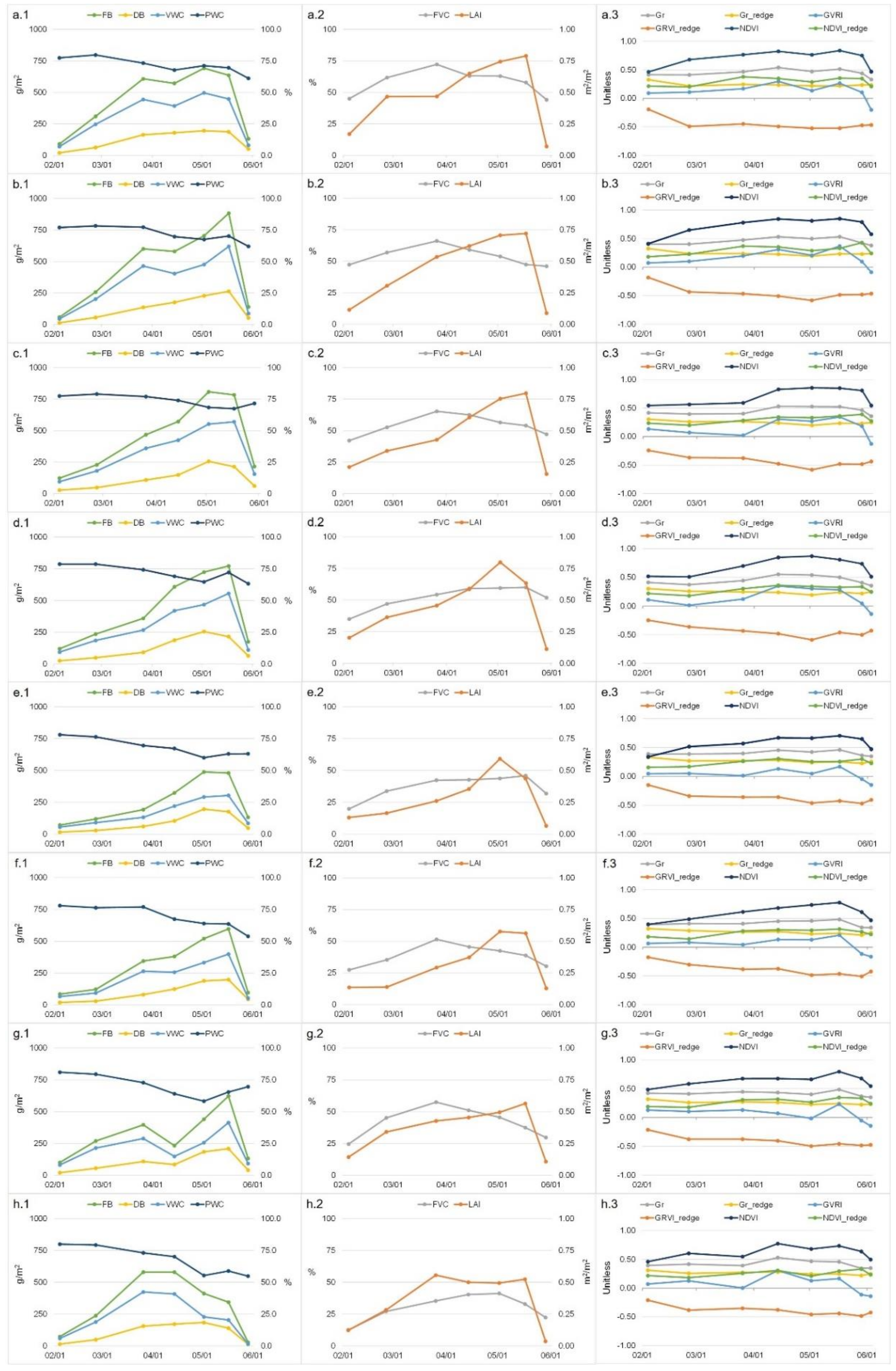
3.1. Spatio-Temporal Patterns

In Appendix A, Figure A1 shows the field estimations and the vegetation indices for the associations on each date of study, whereas Figure A2 shows their temporal evolutions.

3.1.1. Field Measurements

Figure A1 suggested that, as the crop cycle progressed, the values of all field measurements increased progressively on the ordinate axis, until they begun to decrease again as far as the forages approached their maturity point for harvesting. Besides, the associations containing vetch as legume (left side of the figures) showed greater adaptability to edaphoclimatic conditions and, therefore, higher biomass production. Cereal production prevailed over legume production in both cases, which was consistent with the results of other studies [56]. These results are in agreement with those shown graphically in Figure A1 and with those reported by Roberts et al. [57]. On the contrary, the PWC resulted essentially similar for all associations. Therefore, it could be concluded that for an equal consume of water (PWC) in all associations, the vetch-based associations reached considerably higher amounts of plant biomass. This could be of interest to farmers, who seek the highest forage reap while meeting a minimum supply. This result was also supported by the FVC and LAI results, where the vetch associations showed higher canopy coverage and leaf area. This fact is due to the greater tolerance of vetch to the high shading conditions inherent to the cereal-legume polyculture system [58]. Furthermore, it is also relevant the greater susceptibility of pea to attack by bacterial pathogens (Pseudomonas syringae pv. pisi) in high humidity or waterlogged soils [57], as occurred at some stages of the cycle in the PR and PO fields (f.1 in Figure A1). Those fields are located in the lower area of the plot (DEM in Figure 1), prone to become waterlogged.

These results agree well with the analysis of the temporal curve of each association (Figure A2), since higher values of plant biomass were observed in the vetch associations (Figure A2a–d) than in the pea associations, with the greatest differences occurring on dates close to harvest. However, the water consuming remained equal in all associations, as detected in the previous analysis. Additionally, the temporal evolution of the different associations showed a similar growth pattern for all the field parameters studied (except PWC, and to a lesser extent, the FVC), with all the associations showing a plateau-shaped curve [59], typical of the cycle of rainfed crops.

The box plot of the in situ estimations for each association (Figure 3) confirmed the results of the descriptive analysis of Figure A1 and Figure A2. Although the range of those parameters was mainly similar for the eight crop associations, it was detected that the mean values of VBT, VT, VR and VO were slightly higher than those of PBT, PT, PR and PO.

3.1.2. Spectral Indices

The spectral indices followed a similar pattern, i.e., differences between vetch/pea associations were found in all dates, with higher index values for the first ones (Figure A1). In addition, the temporal evolution of the indices (Figure A2) corroborated the temporal behaviour of the field estimations, with a similar plateau-shape, except for the case of the red edge versions.

Based on the analysis of the temporal evolution of each index for the eight associations (Figure A2), it was found that the indices that better followed the different biomass production, VWC and LAI along time seemed to be Gr, NDVI and GRVI. The same abovementioned plateau-shape is evident in them (Figure 3). Hence, it can be expected a plausible way to monitor the associations behaviour through the vegetation indices, as it was explored in next sections. Interestingly, the RGB-based indices showed a similar potential to follow the temporal evolution of plants than the NDVI, even though their dynamic range is smaller (Figure 4), as also found in other applications [60], because the difference in reflectance between the green and red bands for vegetation and soil is small compared with that between near-infrared and red bands [61]. Particularly, the Gr maps (Figure 5) at the tillering (Figure 5a), heading (Figure 5b) and senescence (Figure 5c) followed the expected behaviour of the growing cycle. On the contrary, the three indices based in the red-edge region exhibited a plain temporal evolution (Figure A2) and notably smaller differences between vetch/pea associations.

To correctly interpret the proposed indices, it should be noted that low values of the vegetation-related indices such as GRVI (even negative, in this case), NDVI and Gr indicate limited vegetation activity. On the contrary, when the red-edge band replaces the red one in the GRVI_redge and Gr_redge versions, the lower the index, the greater the plant vigor, as it is expected a higher reflectance of the red-edge band than in the red one for healthy vegetation (Table 2).

3.2. Correlation Analysis

When the dates were analyzed separately (

Table A1. Correlations (n = 16) at each date between field measurements and spectral indices of the eight associations in a whole (Pearson Correlation Coefficient).

Meas. Date	Parameter	FB	DB	VWC	PWC	FCV	LAI	Meas. Date	Parameter	FB	DB	VWC	PWC	FCV	LAI
4 February 2020	Gr	0.244	0.275	0.232	−0.204	0.374	0.265	26 February 2020	Gr	0.173	0.190	0.168	0.036	0.039	0.010
	Gr_redge	−0.587 *	−0.533 *	−0.597 *	−0.111	−0.027	−0.594 *		Gr_redge	−0.618 *	−0.638 **	−0.0610 *	−0.360	−0.715 **	−0.642 **
	GRVI	0.383	0.402	0.373	−0.172	0.316	0.385		GRVI	0.288	0.311	0.281	0.104	0.133	0.108
	GRVI_redge	−0.566 *	−0.530 *	−0.570 *	−0.026	−0.174	−0.593 *		GRVI_redge	−0.641 **	−0.664 **	−0.633 **	−0.361	−0.716 **	−0.635 **
	NDVI	0.512 *	0.512 *	0.506 *	−0.118	0.294	0.555 *		NDVI	0.591 *	0.619 *	0.582 *	0.330	0.594 *	0.497
	NDVI_redge	0.475	0.498 *	0.463	−0.209	0.303	0.577 *		NDVI_redge	0.428	0.461	0.419	0.300	0.639 **	0.399
26 March 2020	Gr	0.399	0.330	0.415	0.231	0.587 *	0.309	14 April 2020	Gr	0.821 **	0.765 **	0.817 **	0.629 **	0.518 *	0.708 **
	Gr_redge	−0.400	−0.292	−0.430	−0.396	−0.597 *	−0.389		Gr_redge	−0.446	−0.426	−0.440	−0.296	−0.836 **	−0.811 **
	GRVI	0.401	0.334	0.417	0.226	0.578 *	0.308		GRVI	0.829 **	0.756 **	0.829 **	0.665 **	0.492	0.673 **
	GRVI_redge	−0.407	−0.307	−0.434	−0.366	−0.621 *	−0.377		GRVI_redge	−0.548 *	−0.530 *	−0.538 *	−0.358	−0.837 **	−0.871 **
	NDVI	0.459	0.390	0.475	0.253	0.655 **	0.340		NDVI	0.836 **	0.782 **	0.830 **	0.616 *	0.675 **	0.848 **
	NDVI_redge	0.627 **	0.573 *	0.634 **	0.239	0.743 **	0.402		NDVI_redge	0.594 *	0.560 *	0.588 *	0.376	0.809 **	0.749 **
2 May 2020	Gr	0.606 *	0.566 *	0.585 *	0.434	0.573 *	0.572 *	17 May 2020	Gr	0.635 **	0.528 *	0.662 **	0.610 *	0.518 *	0.651 **
	Gr_redge	−0.701 **	−0.584 *	−0.699 **	−0.631 **	−0.691 **	−0.638 **		Gr_redge	−0.302	−0.195	−0.336	−0.545 *	−0.483	−0.460
	GRVI	0.606 *	0.576 *	0.581 *	0.429	0.553 *	0.580 *		GRVI	0.742 **	0.639 **	0.766 **	0.643 **	0.504 *	0.698 **
	GRVI_redge	−0.710 **	−0.591 *	−0.708 **	−0.631 **	−0.712 **	−0.643 **		GRVI_redge	−0.297	−0.194	−0.329	−0.517 *	−0.463	−0.452
	NDVI	0.712 **	0.617 *	0.702 **	0.598 *	0.691 **	0.655 **		NDVI	0.597 *	0.499 *	0.622 *	0.628 **	0.459	0.608 *
	NDVI_redge	0.661 **	0.563 *	0.655 **	0.608 *	0.645 **	0.608 *		NDVI_redge	0.501 *	0.457	0.508 *	0.514 *	0.396	0.513 *
29 May 2020	Gr	0.699 **	0.524 *	0.723 **	0.553 *	0.790 **	0.314
	Gr_redge	0.382	0.143	0.454	0.625 **	0.303	−0.075
	GRVI	0.713 **	0.523 *	0.742 **	0.582 *	0.797 **	0.332
	GRVI_redge	0.187	−0.032	0.263	0.521 *	0.021	−0.180
	NDVI	0.582 *	0.478	0.584 *	0.400	0.812 **	0.342
	NDVI_redge	0.266	0.221	0.267	0.234	0.585 *	0.172

** Correlation is significant at the 0.01 level (2-tailed) (Light grey), * Correlation is significant at the 0.05 level (2-tailed) (Dark grey). FB: fresh biomass, DB: dry biomass, VWC: vegetation water content, PWC: percentage of water content, FCV: fraction of vegetation cover, LAI: leaf area index, VBT: vetch-barley-triticale, VT: vetch-triticale, VR: vetch-rye, VO: vetch-oats, PBT: pea-barley-triticale, PT: pea-triticale, PR: pea-rye and PO: pea-oats.

), the correlations were better on the central dates of the cycle (14 April and 2 May), coinciding with the maxima of the growing cycle. This suggested that the observations at the booting and the flowering stages were the best suited to better characterize the state of different associations or crops, as also found in [62]. The best suited indices were NDVI, Gr and GRVI.

Although there seemed to be a clear pattern that distinguishes vetch from pea in the previous exploratory analysis, the correlations at association level did not produce such a difference (

Table A2. Correlations at each association (n = 14) between field measurements and spectral indices along the whole growing cycle (Pearson Correlation Coefficient).

Assoc.	Parameter	FB	DB	VWC	PWC	FVC	LAI	Assoc.	Parameter	FB	DB	VWC	PWC	FVC	LAI
VBT	Gr	0.661 **	0.693 **	0.637 *	−0.203	0.426	0.643 *	PBT	Gr	0.708 **	0.656 *	0.728 **	−0.320	0.474	0.652 *
	Gr_redge	−0.537 *	−0.530	−0.530	0.245	−0.481	−0.553 *		Gr_redge	−0.395	−0.448	−0.352	0.764 **	−0.491	−0.256
	GRVI	0.573 *	0.555 *	0.570 *	−0.003	0.456	0.587 *		GRVI	0.548 *	0.483	0.579 *	−0.075	0.297	0.481
	GRVI_redge	−0.590 *	−0.605 *	−0.573 *	0.325	−0.497	−0.587 *		GRVI_redge	−0.523	−0.562 *	−0.486	0.821 **	−0.604 *	−0.387
	NDVI	0.667 **	0.710 **	0.638 *	−0.423	0.560 *	0.593 *		NDVI	0.682 **	0.680 **	0.670 **	−0.799 **	0.718 **	0.522
	NDVI_redge	0.496	0.585 *	0.452	−0.585 *	0.392	0.254		NDVI_redge	0.427	0.425	0.419	−0.733 **	0.573 *	0.278
VT	Gr	0.700 **	0.741 **	0.678 **	−0.237	0.165	0.771 **	PT	Gr	0.773 **	0.744 **	0.772 **	0.027	0.520	0.713 **
	Gr_redge	−0.422	−0.479	−0.397	0.494	−0.216	−0.459		Gr_redge	−0.366	−0.460	−0.303	0.835 **	−0.191	−0.409
	GRVI	0.729 **	0.747 **	0.715 **	−0.104	0.112	0.790 **		GRVI	0.675 **	0.637 *	0.682 **	0.186	0.415	0.608 *
	GRVI_redge	−0.481	−0.535 *	−0.456	0.504	−0.231	−0.515		GRVI_redge	−0.504	−0.580 *	−0.448	0.814 **	−0.323	−0.526
	NDVI	0.584 *	0.621 *	0.565 *	−0.507	0.185	0.595 *		NDVI	0.846 **	0.872 **	0.812 **	−0.596 *	0.578 *	0.809 **
	NDVI_redge	0.213	0.234	0.203	−0.634 *	0.078	0.152		NDVI_redge	0.731 **	0.736 **	0.711 **	−0.570 *	0.569 *	0.697 **
VR	Gr	0.660 *	0.683 **	0.645 *	−0.792 **	0.209	0.676 **	PR	Gr	0.688 **	0.579 *	0.729 **	−0.064	0.331	0.614 *
	Gr_redge	−0.550 *	−0.580 *	−0.532	0.817 **	−0.328	−0.551 *		Gr_redge	−0.368	−0.452	−0.299	0.663 **	−0.195	−0.279
	GRVI	0.654 *	0.683 **	0.636 *	−0.725 **	0.061	0.658 *		GRVI	0.530	0.373	0.609 *	0.247	0.186	0.398
	GRVI_redge	−0.584 *	−0.606 *	−0.570 *	0.834 **	−0.359	−0.576 *		GRVI_redge	−0.452	−0.536 *	−0.380	0.733 **	−0.281	−0.390
	NDVI	0.631 *	0.658 *	0.615 *	−0.887 **	0.199	0.589 *		NDVI	0.721 **	0.723 **	0.689 **	−0.638 *	0.421	0.580 *
	NDVI_redge	0.499	0.519	0.486	−0.817 **	0.189	0.380		NDVI_redge	0.438	0.492	0.384	−0.644 *	0.275	0.323
VO	Gr	0.841 **	0.854 **	0.817 **	−0.319	0.735 **	0.732 **	PO	Gr	0.653 *	0.704 **	0.586 *	−0.028	0.613 *	0.641 *
	Gr_redge	−0.566 *	−0.679 **	−0.498	0.802 **	−0.771 **	−0.496		Gr_redge	0.156	−0.020	0.231	0.743 **	−0.214	0.065
	GRVI	0.823 **	0.807 **	0.814 **	−0.174	0.678 **	0.704 **		GRVI	0.548 *	0.537 *	0.518	0.193	0.435	0.537 *
	GRVI_redge	−0.653 *	−0.750 **	−0.591 *	0.793 **	−0.838 **	−0.557 *		GRVI_redge	−0.086	−0.279	0.012	0.794 **	−0.445	−0.164
	NDVI	0.797 **	0.845 **	0.756 **	−0.631 *	0.872 **	0.630 *		NDVI	0.413	0.532	0.329	−0.508	0.569 *	0.429
	NDVI_redge	0.603 *	0.673 **	0.555 *	−0.727 **	0.769 **	0.400		NDVI_redge	0.062	0.064	0.058	−0.454	0.077	−0.034

** Correlation is significant at the 0.01 level (2-tailed) (Light grey), * Correlation is significant at the 0.05 level (2-tailed) (Dark grey). FB: fresh biomass, DB: dry biomass, VWC: vegetation water content, PWC: percentage of water content, FCV: fraction of vegetation cover, LAI: leaf area index, VBT: vetch-barley-triticale, VT: vetch-triticale, VR: vetch-rye, VO: vetch-oats, PBT: pea-barley-triticale, PT: pea-triticale, PR: pea-rye and PO: pea-oats.

), since no remarkable differences in the correlation values were found along associations. However, it should be noted that the Pearson coefficient seeks for a similar behavior, ignoring the absolute values. Thus, it would be inferred that the temporal behavior was similar between associations (as already seen in Figure A2), even though the higher vetch yields.

Since the associations are a mix of different plants, all of them with different growing characteristics (e.g., different foliage, height and density), the vegetation indices did not reach saturation, which typically occurs for dense vegetation coverages of single canopies with the remotely sensed NDVI [35,63], and it was also observed for the UAV-based GRVI for biomass greater than 150 g/m² in corn and soybean [61] and in wheat [62]. In such scenarios, the correlation declines due to the saturation of the index at some point, which is not the case here. This fact may explain the higher correlation as regard of other similar works on drone vegetation indices for monitoring individual plant species [49,50]. In addition, removing the influence of lighting changes and solar reflection angle is particularly necessary for the RGB images [51,64], used here to calculate the indices. The sun-downlight correction and the reflectance calibration applied to the Micasense images could have been improved the results of correlation, as regards of other similar research in which RGB indices were correlated with biomass and LAI [49].

As regard of the associations, the worst characterized was PO, while the best was VO (Table A2). The most difficult parameter to monitor was FVC. The indices that correlated best with the temporal evolution were NDVI, Gr and GRVI. On the contrary, the indices based in the red-edge band did not perform well and also had a negative correlation due to their inverse behavior, which makes their interpretation difficult. However, other studies have revealed the red-edge NDVI as a good indicator of Nitrogen level over rice fields [65] as well as other chemical parameters of corn [66]. The relationship of the red-edge indices with other different parameters as the chlorophyll content will be explored in further research in the same area. In this work, the bad results of the red edge-based indices to depict structural parameters such as LAI and biomass could be due to an inadequate replacement of the red band for the red edge one in the indices formulation, especially in the Gr_redge and GRVI_edge cases. The higher reflectance of the red edge band than that of the green one for vigorous plants led to unwanted results in their calculation (Table 2).

Correlations were very strong and significant for each association throughout their growing cycle (Table A2), suggesting that the evolution of the associations would be monitored from the spectral indices. These high correlations invited an attempt at more complex statistical modeling to predict plant behavior based on the indices, as done in the next section.

3.3. Modeling and Prediction of the Associations Behaviour PLS Regression

An attempt to model the associations time evolution was carried out by means of a PLS regression. The PLS-regression model is one of the least restrictive of all classical multivariate regression models. Due to this fact, it can be used to predict in situations where other models are limited. In particular, it is appropriated when there are fewer observations than predictor variables, which is a common situation in drone applications, where the image analysis affords a large set of predictor variables whereas the ground observations to fit the models are usually scarce. Several examples of these PLS regression predictive applications in precision agriculture can be found in Nguyen et al. [67], Abdel-Rahman et al. [68] and more recently in Kawamura [69], Erler et al. [70] and Helfer et al. [31].

In the same way, our final aim was to predict the field parameters at any time of the growing cycle with the sole input of the vegetation indices. To test this objective, and to account for the previous exploratory results, three variants of the PLS analysis were proposed, i.e., a global one considering all the associations as a whole, and another two PLS for the associations based in vetch (VBT, VT, VR and VO) and in pea (PBT, PT, PR and PO).

3.3.1. Global PLS Analysis for All Associations as a Whole

The first PLS regression used data from all crop associations treated simultaneously.

Table 3. Capability of explanatory ($X$) and response variables ($Y$) of VBT, VT, VR, VO, PBT, PT, PR and PO associations to capture % of variance depending on the number of components. Predictive potential expressed as $R^2$.

$\mathbf{Component}\left(\mathbf{h}\right)$	% Variance	% Accumulated	% Variance	% Accumulated	Mean Predicted
	$\mathit{X}$	$\mathit{X}$	$\mathit{Y}$	$\mathit{Y}$	${\mathit{R}}^2$
1	69.94	69.94	44.43	44.44	42.50
2	22.09	92.03	7.01	51.45	48.74
3	7.13	99.16	2.07	53.52	49.97
4	0.51	99.67	4.23	57.75	53.38
5	0.32	99.99	0.34	58.09	53.06
6	0.01	100.00	1.13	59.22	52.83

VBT: vetch-barley-triticale, VT: vetch-triticale, VR: vetch-rye, VO: vetch-oats, PBT: pea-barley-triticale, PT: pea-triticale, PR: pea-rye and PO: pea-oats.

shows $X$ (vegetation indices of all associations) and $Y$ (field measurements of all associations) capability to capture the relevant information, expressed as % of variance, with the subsequent mean predicted value $R^2$ depending on the number of extracted components by the PLS regression model. In view of these results, a regression model based solely on the first four components was constructed. Firstly, because the predictive value $R^2$ remains nearly stable from the fourth component onwards. Besides, a greater number of components would lead to a model with more parameters and complexity while similar predictive capacity. With four components the model was able to explain 99.67% of the variability of the explanatory variables and 57.75% of the variability of the response variables. It was noteworthy that the first component explained a higher percentage of the variability of $X$ and, with just two components, more than 90% of this variability was explained. The mean predictive capacity ($R^2$) after the LOOCV was 53.38%. In other words, the six explanatory variables provided by the multispectral images captured by the drone were sufficient to predict more than 50% of the field parameters. However, a model with a single component also provided significant levels of prediction $\left(R^2=42.50\right)$. Hence, some redundancy between the vegetation indices (the explanatory variables) was detected. This is not surprising, since the vegetation indices formulation (Table 2) was based in a combination of the same bands in the VNIR spectra. Far for being a problem, this result afforded two main advantages of our hypothesis: (1) PLS regression was able to deal with multicollinearity in data and eliminate the less important or redundant variables, as also found in Zhou et al. [29], and (2) a single combination of VNIR bands, or even visible bands solely, was able to feed the regression model, leading to a successful prediction of the agronomic parameters.

Table 4. Predictive capacity of the PLS analysis for each of the response variables of VBT, VT, VR, VO, PBT, PT, PR and PO associations for four components.

Explanatory		Mean	Predicted
Variable	${\mathit{R}}^2$	PRESS	${\mathit{R}}^2$
FB (g/m2)	65.75	22,520.30	62.23
DB (g/m2)	70.40	2017.47	67.07
VWC (g/m2)	61.12	12,493.50	57.32
PWC (%)	52.47	31.23	47.34
LAI (m2/m2)	62.02	0.02	57.79
FVC (%)	34.77	133.34	28.54

FB: fresh biomass, DB: dry biomass, VWC: vegetation water content, PWC: percentage of water content, LAI: leaf area index, FCV: fraction of vegetation cover, VBT: vetch-barley-triticale, VT: vetch-triticale, VR: vetch-rye, VO: vetch-oats, PBT: pea-barley-triticale, PT: pea-triticale, PR: pea-rye and PO: pea-oats.

shows the predictive capacity of the global PLS analysis with four components for each of the response variables, and Figure 5 shows the plots of observed vs. predicted values for each of the six response variables of all associations considering a four-component model. Overall, a strong dependency relationship was detected between the explanatory and observed variables, with a remarkable predictive capacity for LAI ($R^2=57.79$), FB ($R^2=62.63$), DB ($R^2=67.07$), VWC ($R^2=57.32$) and PWC ($R^2=47.34$). The relationship seemed to be linear in all cases (Figure 6) excepting for FVC, in which the prediction ($R^2=28.54$) was notably lower than for the rest of the variables and with no evident linear relationship (Figure 6f).

In similar research [29] it was proven that the PLS performed better under linearity conditions and with a number of predictor variables equal or greater than the number of predicted variables, as it was the case here. For no linear relationships, the SVM was preferred [71,72].

3.3.2. PLS Analysis for the Vetch-Based Associations (VBT, VT, VR and VO)

Table 5. Capability of explanatory ($X$) and response variables ($Y$) of VBT, VT, VR and VO associations to capture % of variance depending on the number of components. Predictive potential expressed as $R^2$.

$\mathbf{Component}\left(\mathbf{h}\right)$	% Variance	% Accumulated	% Variance	% Accumulated	Mean Predicted
	$\mathit{X}$	$\mathit{X}$	$\mathit{Y}$	$\mathit{Y}$	${\mathit{R}}^2$
1	76.03	76.03	44.15	44.15	40.81
2	12.58	88.61	8.29	52.45	45.97
3	10.67	99.28	1.63	54.08	46.42
4	0.51	99.89	2.10	56.18	46.37
5	0.18	99.98	0.63	56.82	45.74
6	0.02	100.00	3.18	60.01	47.85

VBT: vetch-barley-triticale, VT: vetch-triticale, VR: vetch-rye and VO: vetch-oats.

shows the percentage of variance retained by the explanatory variables ($X$) and by the response variables ($Y$). In this case, the regression model was based on the first three components, and was able to explain 99.28% of the variability of the explanatory variables and 54.08% of the variability of the response variables. The mean predictive capacity ($R^2$) after the LOOCV was 46.42%. This $R^2$ value was slightly lower than that obtained in the global analysis (53.38%), probably due to its smaller amount of data.

The predictive capacity of the PLS analysis for each response variable for three components (

Table 6. Predictive capacity of the PLS analysis for each of the response variables of VBT, VT, VR and VO associations for three components.

Explanatory		Mean	Predicted
Variable	${\mathit{R}}^2$	PRESS	${\mathit{R}}^2$
FB (g/m2)	62.65	31,210.60	56.77
DB (g/m2)	67.90	2590.51	62.71
VWC (g/m2)	58.26	17,213.00	51.74
PWC (%)	49.11	22.17	38.90
LAI (m2/m2)	64.09	0.03	58.86
FVC (%)	22.49	81.60	9.50

FB: fresh biomass, DB: dry biomass, VWC: vegetation water content, PWC: percentage of water content, LAI: leaf area index and FCV: fraction of vegetation cover, VBT: vetch-barley-triticale, VT: vetch-triticale, VR: vetch-rye and VO: vetch-oats.

) was lower than in the global analysis in terms of the predicted $R^2$. Again, FVC was the worst predicted, this time with a clearly worse $R^2$ of 9.50. This bad result is difficult to interpret, since LAI and FB, typically related with FVC [38], reached good performances both in the correlation analysis and in their prediction capability. Two explanations may arise. Firstly, the time-lag found between the FVC curve and the rest of parameters and indices (occurring at five out of the height associations, see Figure A2), coinciding with the findings of Sánchez et al. [38] for grass coverages. Second, the methodology to estimate the FVC from the classification of zenithal photographs may be questionable when the canopy is a mix of species with different coloration, as found by Calera et al. [43].

3.3.3. PLS Analysis for the Pea-Based Associations (PBT, PT, PR and PO)

Although the results in

Table 7. Capability of explanatory ($X$) and response variables ($Y$) of PBT, PT, PR and PO associations to capture % of variance depending on the number of components. Predictive potential expressed as $R^2$.

$\mathbf{Component}\left(\mathbf{h}\right)$	% Variance	% Accumulated	% Variance	% Accumulated	Mean Predicted
	$\mathit{X}$	$\mathit{X}$	$\mathit{Y}$	$\mathit{Y}$	${\mathit{R}}^2$
1	54.70	54.70	41.70	41.70	37.02
2	37.43	92.14	8.10	49.81	44.29
3	6.86	99.01	1.83	51.65	44.92
4	0.82	99.8	5.81	57.46	48.62
5	0.15	99.99	1.65	59.11	48.97
6	0.01	100.000	3.70	62.82	49.80

PBT: pea-barley-triticale, PT: pea-triticale, PR: pea-rye and PO: pea-oats.

were similar to those obtained in the previous scenario with the vetch associations, two slight differences should be noted: on the one hand, the variability of $X$ was better distributed between the first and second components (92.14% vs. 88.61%) and, on the other hand, a four-component model, just like in the global analysis, could be chosen in this case, because the mean predicted $R^2$ increased slightly between the third ($R^2=44.92$) and fourth ($R^2=48.62$) components.

As in the previous case, the prediction model for the FVC variable showed the lowest $R^2$ (

Table 8. Predictive capacity of the PLS analysis for each of the response variables of PBT, PT, PR and PO associations for four components.

Explanatory		Mean	Predicted
Variable	${\mathit{R}}^2$	PRESS	${\mathit{R}}^2$
FB (g/m2)	62.19	16,471.20	54.89
DB (g/m2)	69.70	1802.05	63.16
VWC (g/m2)	54.96	8598.87	46.65
PWC (%)	66.10	30.90	59.36
LAI (m2/m2)	58.21	0.02	48.68
FVC (%)	33.61	101.64	18.99

FB: fresh biomass, DB: dry biomass, VWC: vegetation water content, PWC: percentage of water content, LAI: leaf area index, FCV: fraction of vegetation cover, PBT: pea-barley-triticale, PT: pea-triticale, PR: pea-rye and PO: pea-oats.

). On the other hand, the PWC variable was now notably better explained $\left(R^2=59.36 vs. R^2=38.90\right)$. As in the vetch model, the mean predictive $R^2$ value is slightly lower than that obtained in the global analyses (48.62% vs. 53.38%).

4. Conclusions

Camera-based VNIR vegetation indices on board UAVs platforms could offer an effective and affordable alternative to field-consuming, destructive sampling to monitor crops. This methodology, together with the support of statistical modeling techniques have shown a high capability of monitoring and predicting the behavior of height forage associations.

The exploratory analysis, together with the correlation analysis, exhibited a strong relationship between the spectral indices and the field estimations, suggesting a further prediction model. Owing the linearity found in these relationships, a simple regressive prediction model (PLS) was proposed.

The vetch-based and the pea-based associations showed a different behavior both at the field and image estimations. While the water consuming was similar for both, biomass production was higher for the first, which may be a useful result for farmers seeking the highest forage production. Interestingly, the spectral indices were also able to detect this behavior, offering an alternative way to evaluate both the production and the use of water of their crops.

Using a reduced number of multispectral observations (in the form of vegetation indices) and applying the PLS model, we were able to predict agronomic parameters of forage crop associations at any time of their cycle with a reliability of more than 50%. In fact, six indices were integrated in the model, but it was sown that they provided redundant information. Therefore, they could have been reduced by half, since the red edge-based indices were not satisfactory in the exploratory and correlation analysis. An alternative use of the red edge indices should be explored in further research, both in their formulation and in their relationships with other observed parameters, such chlorophyll. On the contrary, the indices Gr and GVRI, based in the green and red bands, correlated well with the field parameters and revealed a similar capacity to predict the temporal behaviour than the NDVI, with the advantage of being easier to acquire through the RGB cameras, typically onboard UAVs.

Overall, a strong, linear dependency relationship was detected between the explanatory and the observed variables, with a remarkable predictive capacity. This predictive capacity could be refined avoiding the redundant information while adding new explanatory variables such as other vegetation indices. In addition, other parameters such as yield and chlorophyll content will be explored in the future.

References

1. Ghanbari-Bonjar, A.; Lee, H.C. Intercropped wheat (Triticum aestivum L.) and bean (Vicia faba L.) as a whole-crop forage: Effect of harvest time on forage yield and quality. Grass Forage Sci. 2003, 58, 28–36. [Google Scholar] [CrossRef]
2. Nadeem, M.; Ansar, M.; Anwar, A.; Hussain, A. Performance of Winter Cereal-Legumes Fodder Mixtures and Their Pure Stand at Different Growth Stages Under Rainfed Conditions of Pothowar. J. Agric. Res. 2010, 48, 181–192. [Google Scholar]
3. Eskandari, H.; Ghanbari, A.; Javanmard, A. Intercropping of Cereals and Legumes for Forage Production. Not. Sci. Biol. 2009, 1, 07–13. [Google Scholar] [CrossRef] [Green Version]
4. Willey, R.W. Intercropping: Its Importance and Research Needs. Part 1, Competition and Yield Advantages. Field Crop. Abstr. 1979, 32, 1–10. [Google Scholar]
5. Staniak, M.; Ksiak, J.; Bojarszczuk, J. Mixtures of Legumes with Cereals as a Source of Feed for Animals. In Organic Agriculture Towards Sustainability; Pilipavicius, V., Ed.; InTech: Kaunas, Lithuania, 2014; pp. 123–145. ISBN 978-953-51-1340-9. [Google Scholar]
6. Chandel, A.K.; Khot, L.R.; Yu, L.-X. Alfalfa (Medicago sativa L.) crop vigor and yield characterization using high-resolution aerial multispectral and thermal infrared imaging technique. Comput. Electron. Agric. 2021, 182, 105999. [Google Scholar] [CrossRef]
7. Undersander, D.; Grau, C.; Cosgrove, D.; Doll, J.; Martin, N. Alfalfa Stand Assessment: Is This Stand Good Enough to Keep? University of Wisconsin-Extension: Madison, WI, USA, 2011; pp. 3–6. [Google Scholar]
8. Puangbut, D.; Jogloy, S.; Vorasoot, N. Association of photosynthetic traits with water use efficiency and SPAD chlorophyll meter reading of Jerusalem artichoke under drought conditions. Agric. Water Manag. 2017, 188, 29–35. [Google Scholar] [CrossRef]
9. Pereira, L.S.; Paredes, P.; Melton, F.; Johnson, L.; Wang, T.; López-Urrea, R.; Cancela, J.J.; Allen, R.G. Prediction of Crop Coefficients from Fraction of Ground Cover and Height. Background and Validation Using Ground and Remote Sensing Data; Elsevier B.V.: Amsterdam, The Netherlands, 2020; Volume 241. [Google Scholar]
10. Guan, J.; Nutter, F.W. Relationships between defoliation, leaf area index, canopy reflectance, and forage yield in the alfalfa-leaf spot pathosystem. Comput. Electron. Agric. 2003, 37, 97–112. [Google Scholar] [CrossRef]
11. Orloff, S.B. Methods to assess alfalfa forage quality in the field. In Proceedings of the 27th National Alfalfa Symposium, San Diego, CA, USA, 9–10 December 1996; pp. 183–193. [Google Scholar]
12. Salama, H.S.A. Mixture cropping of berseem clover with cereals to improve forage yield and quality under irrigated conditions of the Mediterranean basin. Ann. Agric. Sci. 2020, 65, 159–167. [Google Scholar] [CrossRef]
13. Mulla, D.J. Twenty five years of remote sensing in precision agriculture: Key advances and remaining knowledge gaps. Biosyst. Eng. 2013, 114, 358–371. [Google Scholar] [CrossRef]
14. Chang, A.; Jung, J.; Maeda, M.M.; Landivar, J. Crop height monitoring with digital imagery from Unmanned Aerial System (UAS). Comput. Electron. Agric. 2017, 141, 232–237. [Google Scholar] [CrossRef]
15. Pádua, L.; Vanko, J.; Hruška, J.; Adão, T.; Sousa, J.J.; Peres, E.; Morais, R. UAS, sensors, and data processing in agroforestry: A review towards practical applications. Int. J. Remote Sens. 2017, 38, 2349–2391. [Google Scholar] [CrossRef]
16. Li, X.; Lee, W.S.; Li, M.; Ehsani, R.; Mishra, A.R.; Yang, C.; Mangan, R.L. Spectral difference analysis and airborne imaging classification for citrus greening infected trees. Comput. Electron. Agric. 2012, 83, 32–46. [Google Scholar] [CrossRef]
17. Verger, A.; Vigneau, N.; Chéron, C.; Gilliot, J.M.; Comar, A.; Baret, F. Green area index from an unmanned aerial system over wheat and rapeseed crops. Remote Sens. Environ. 2014, 152, 654–664. [Google Scholar] [CrossRef]
18. Zhou, X.; Zheng, H.B.; Xu, X.Q.; He, J.Y.; Ge, X.K.; Yao, X.; Cheng, T.; Zhu, Y.; Cao, W.X.; Tian, Y.C. Predicting grain yield in rice using multi-temporal vegetation indices from UAV-based multispectral and digital imagery. ISPRS J. Photogramm. Remote Sens. 2017, 130, 246–255. [Google Scholar] [CrossRef]
19. Castro, W.; Junior, J.M.; Polidoro, C.; Osco, L.P.; Gonçalves, W.; Rodrigues, L.; Santos, M.; Jank, L.; Barrios, S.; Valle, C.; et al. Deep Learning Applied to Phenotyping of Biomass in Forages with Uav-Based RGB Imagery. Sensors 2020, 20, 4802. [Google Scholar] [CrossRef]
20. Rouse, J.W.; Haas, R.H.; Schell, J.A.; Deering, D.W.; Harlan, J.C. Monitoring the Vernal Advancement and Retrogradation (Green Wave Effect) of Natural Vegetation. In Final Report, Type III; NASA/GSFC: Greenbelt, MD, USA, 1974; p. 371. [Google Scholar]
21. Becker-Reshef, I.; Vermote, E.; Lindeman, M.; Justice, C. A generalized regression-based model for forecasting winter wheat yields in Kansas and Ukraine using MODIS data. Remote Sens. Environ. 2010, 114, 1312–1323. [Google Scholar] [CrossRef]
22. Maresma, A.; Chamberlain, L.; Tagarakis, A.; Kharel, T.; Godwin, G.; Czymmek, K.J.; Shields, E.; Ketterings, Q.M. Accuracy of NDVI-derived corn yield predictions is impacted by time of sensing. Comput. Electron. Agric. 2020, 169, 105236. [Google Scholar] [CrossRef]
23. Shafiee, S.; Lied, L.M.; Burud, I.; Dieseth, J.A.; Alsheikh, M.; Lillemo, M. Sequential forward selection and support vector regression in comparison to LASSO regression for spring wheat yield prediction based on UAV imagery. Comput. Electron. Agric. 2021, 183, 106036. [Google Scholar] [CrossRef]
24. Drucker, H.; Burges, C.J.C.; Kaufman, L.; Smola, A.; Vapnik, V. Support Vector Regression Machines. In Advances in Neural Information Processing Systems 9; MIT Press: Cambridge, MA, USA, 1997; pp. 155–161. [Google Scholar]
25. Wold, H. Soft modelling: The Basic Design and Some Extensions. In Systems Under Indirect Observation: Causality-Structure-Prediction. Part II; North-Holland Publishing Company: Amsterdam, The Netherlands, 1982; pp. 1–54. [Google Scholar]
26. Wold, S.; Sjöström, M.; Eriksson, L. PLS-regression: A basic tool of chemometrics. Chemom. Intell. Lab. Syst. 2001, 58, 109–130. [Google Scholar] [CrossRef]
27. Ma, D.; Maki, H.; Neeno, S.; Zhang, L.; Wang, L.; Jin, J. Application of non-linear partial least squares analysis on prediction of biomass of maize plants using hyperspectral images. Biosyst. Eng. 2020, 200, 40–54. [Google Scholar] [CrossRef]
28. Montes, J.M.; Technow, F.; Dhillon, B.S.; Mauch, F.; Melchinger, A.E. High-throughput non-destructive biomass determination during early plant development in maize under field conditions. Field Crops Res. 2011, 121, 268–273. [Google Scholar] [CrossRef]
29. Zhou, Z.; Morel, J.; Parsons, D.; Kucheryavskiy, S.V.; Gustavsson, A.-M. Estimation of yield and quality of legume and grass mixtures using partial least squares and support vector machine analysis of spectral data. Comput. Electron. Agric. 2019, 162, 246–253. [Google Scholar] [CrossRef]
30. Osborne, S.L.; Schepers, J.S.; Francis, D.D.; Schlemmer, M.R. Use of Spectral Radiance to Estimate In-Season Biomass and Grain Yield in Nitrogen- and Water-Stressed Corn. Crop. Sci. 2002, 42, 165–171. [Google Scholar] [PubMed]
31. Helfer, G.A.; Victória Barbosa, J.L.; dos Santos, R.; da Costa, A.B. A computational model for soil fertility prediction in ubiquitous agriculture. Comput. Electron. Agric. 2020, 175, 105602. [Google Scholar] [CrossRef]
32. Abdi, H. Partial least squares regression and projection on latent structure regression (PLS Regression). WIREs Comput. Stat. 2010, 2, 97–106. [Google Scholar] [CrossRef]
33. Krishnan, A.; Williams, L.J.; McIntosh, A.R.; Abdi, H. Partial Least Squares (PLS) methods for neuroimaging: A tutorial and review. NeuroImage 2011, 56, 455–475. [Google Scholar] [CrossRef]
34. Barnsley, M.J.; Lewis, P.; O’Dwyer, S.; Disney, M.I.; Hobson, P.; Cutter, M.; Lobb, D. On the potential of CHRIS/PROBA for estimating vegetation canopy properties from space. Remote Sens. Rev. 2000, 19, 171–189. [Google Scholar] [CrossRef]
35. Jackson, T.J.; Chen, D.; Cosh, M.; Li, F.; Anderson, M.; Walthall, C.; Doriaswamy, P.; Hunt, E.R. Vegetation water content mapping using Landsat data derived normalized difference water index for corn and soybeans. Remote Sens. Environ. 2004, 92, 475–482. [Google Scholar] [CrossRef]
36. Jiang, Z.; Huete, A.R.; Chen, J.; Chen, Y.; Li, J.; Yan, G.; Zhang, X. Analysis of NDVI and scaled difference vegetation index retrievals of vegetation fraction. Remote Sens. Environ. 2006, 101, 366–378. [Google Scholar] [CrossRef]
37. Valcarce-Diñeiro, R.; Lopez-Sanchez, J.M.; Sánchez, N.; Arias-Pérez, B.; Martínez-Fernández, J. Influence of Incidence Angle in the Correlation of C-band Polarimetric Parameters with Biophysical Variables of Rain-fed Crops. Can. J. Remote Sens. 2018, 44, 643–659. [Google Scholar] [CrossRef]
38. Sánchez, N.; Martínez-Fernández, J.; González-Piqueras, J.; González-Dugo, M.P.; Baroncini-Turrichia, G.; Torres, E.; Calera, A.; Pérez-Gutiérrez, C. Water balance at plot scale for soil moisture estimation using vegetation parameters. Agric. For. Meteorol. 2012, 166–167, 1–9. [Google Scholar] [CrossRef]
39. Abràmoff, M.D.; Magalhães, P.J.; Ram, S.J. Image Processing with Image. J. Biophotonics Int. 2004, 11, 36–42. [Google Scholar]
40. Martin, T.N.; Marchese, J.A.; Fernandes de Sousa, A.K.; Curti, G.L.; Fogolari, H.; Dos Santos, V. Using the imagej software to estimate leaf area in bean crop. Interciencia 2013, 38, 843–848. [Google Scholar]
41. García-Estévez, I.; Quijada-Morín, N.; Rivas-Gonzalo, J.C.; Martínez-Fernández, J.; Sánchez, N.; Herrero-Jiménez, C.M.; Escribano-Bailón, M.T. Relationship between hyperspectral indices, agronomic parameters and phenolic composition of Vitis vinifera cv Tempranillo grapes: Hyperspectral indices, agronomic parameters and phenolic composition of V. vinifera. J. Sci. Food Agric. 2017, 97, 4066–4074. [Google Scholar] [CrossRef] [Green Version]
42. Abdelkader, M.M.M.; Puchkov, M.; Loktionova, E. Applying a digital method for measuring leaf area index of tomato plants. In Proceedings of the International Scientific and Practical Conference “Digital agriculture—Development strategy” (ISPC 2019), Ekaterinburg, Russia, 21–22 March 2019; Atlantis Press: Ekaterinburg, Russia, 2019. [Google Scholar]
43. Calera, A.; Martínez, C.; Melia, J. A procedure for obtaining green plant cover: Relation to NDVI in a case study for barley. Int. J. Remote Sens. 2001, 22, 3357–3362. [Google Scholar] [CrossRef]
44. Tucker, C.J. Red and photographic infrared linear combinations for monitoring vegetation. Remote Sens. Environ. 1979, 8, 127–150. [Google Scholar] [CrossRef] [Green Version]
45. Sánchez, N.; Alonso-Arroyo, A.; Martínez-Fernández, J.; Piles, M.; González-Zamora, Á.; Camps, A.; Vall-llosera, M. On the Synergy of Airborne GNSS-R and Landsat 8 for Soil Moisture Estimation. Remote Sens. 2015, 7, 9954–9974. [Google Scholar] [CrossRef] [Green Version]
46. Hunt, E.R.; Doraiswamy, P.C.; McMurtrey, J.E.; Daughtry, C.S.T.; Perry, E.M.; Akhmedov, B. A visible band index for remote sensing leaf chlorophyll content at the Canopy scale. Int. J. Appl. Earth Obs. Geoinform. 2013, 21, 103–112. [Google Scholar] [CrossRef] [Green Version]
47. Sumesh, K.C.; Ninsawat, S.; Som-ard, J. Integration of RGB-based vegetation index, crop surface model and object-based image analysis approach for sugarcane yield estimation using unmanned aerial vehicle. Comput. Electron. Agric. 2021, 180, 105903. [Google Scholar] [CrossRef]
48. Khan, Z.; Rahimi-Eichi, V.; Haefele, S.; Garnett, T.; Miklavcic, S.J. Estimation of vegetation indices for high-throughput phenotyping of wheat using aerial imaging. Plant. Methods 2018, 14, 20. [Google Scholar] [CrossRef] [PubMed]
49. Jannoura, R.; Brinkmann, K.; Uteau, D.; Bruns, C.; Joergensen, R.G. Monitoring of crop biomass using true colour aerial photographs taken from a remote controlled hexacopter. Biosyst. Eng. 2015, 129, 341–351. [Google Scholar] [CrossRef]
50. Lussem, U.; Bolten, A.; Gnyp, M.L.; Jasper, J.; Bareth, G. Evaluation of RGB-based vegetation indices from UAV imagery to estimate forage yield in grassland. ISPRS Int. Arch. Photogramm. Remote Sens. Spat. Inf. Sci. 2018, XLII–3, 1215–1219. [Google Scholar] [CrossRef] [Green Version]
51. Barbosa, B.D.S.; Ferraz, G.a.S.; Gonçalves, L.M.; Marin, D.B.; Maciel, D.T.; Ferraz, P.F.P.; Rossi, G. RGB vegetation indices applied to grass monitoring: A qualitative analysis. Agron. Res. 2019, 17, 2. [Google Scholar] [CrossRef]
52. Bendig, J.; Yu, K.; Aasen, H.; Bolten, A.; Bennertz, S.; Broscheit, J.; Gnyp, M.L.; Bareth, G. Combining UAV-based plant height from crop surface models, visible, and near infrared vegetation indices for biomass monitoring in barley. Int. J. Appl. Earth Obs. Geoinform. 2015, 39, 79–87. [Google Scholar] [CrossRef]
53. Sripada, R.P.; Heiniger, R.W.; White, J.G.; Meijer, A.D. Aerial Color Infrared Photography for Determining Early In-Season Nitrogen Requirements in Corn. Agron. J. 2006, 98, 968–977. [Google Scholar] [CrossRef]
54. Motohka, T.; Nasahara, K.N.; Oguma, H.; Tsuchida, S. Applicability of Green-Red Vegetation Index for Remote Sensing of Vegetation Phenology. Remote Sens. 2010, 2, 2369–2387. [Google Scholar] [CrossRef] [Green Version]
55. Pearson, K. On the Theory of Contingency and Its Relation to Association and Normal Correlation; Dulau and Company: London, UK, 1904; Volume 1, p. 46. [Google Scholar]
56. Hauggaard-Nielsen, H.; Jensen, E.S. Evaluating pea and barley cultivars for complementarity in intercropping at different levels of soil N availability. Field Crops Res. 2001, 72, 185–196. [Google Scholar] [CrossRef]
57. Roberts, S.J. Effect of soil moisture on the transmission of pea bacterial blight (Pseudomonas syringae pv. pisi) from seed to seedling. Plant. Pathol. 1992, 41, 136–140. [Google Scholar] [CrossRef]
58. Li, R.; Zhang, Z.; Tang, W.; Huang, Y.; Coulter, J.A.; Nan, Z. Common vetch cultivars improve yield of oat row intercropping on the Qinghai-Tibetan plateau by optimizing photosynthetic performance. Eur. J. Agron. 2020, 117, 126088. [Google Scholar] [CrossRef]
59. Calera, A.; González-Piqueras, J.; Melia, J. Monitoring barley and corn growth from remote sensing data at field scale. Int. J. Remote Sens. 2004, 25, 97–109. [Google Scholar] [CrossRef]
60. Gutierrez, M.; Escalante Estrada, J.A.; And, E.-E.; Rodriguez-Gonzalez, M. Canopy Reflectance, Stomatal Conductance, and Yield of Phaseolus vulgaris L. and Phaseolus coccinues L. Under Saline Field Conditions. Int. J. Agric. Biol. 2005, 7, 491–494. [Google Scholar]
61. Hunt, E.R.; Cavigelli, M.; Daughtry, C.S.T.; Mcmurtrey, J.E.; Walthall, C.L. Evaluation of Digital Photography from Model Aircraft for Remote Sensing of Crop Biomass and Nitrogen Status. Precis. Agric. 2005, 6, 359–378. [Google Scholar] [CrossRef]
62. Fu, Z.; Jiang, J.; Gao, Y.; Krienke, B.; Wang, M.; Zhong, K.; Cao, Q.; Tian, Y.; Zhu, Y.; Cao, W.; et al. Wheat Growth Monitoring and Yield Estimation based on Multi-Rotor Unmanned Aerial Vehicle. Remote Sens. 2020, 12, 508. [Google Scholar] [CrossRef] [Green Version]
63. Gamon, J.A.; Field, C.B.; Goulden, M.L.; Griffin, K.L.; Hartley, A.E.; Joel, G.; Peñuelas, J.; Valentini, R. Relationships Between NDVI, Canopy Structure, and Photosynthesis in Three Californian Vegetation Types. Ecol. Appl. 1995, 5, 28–41. [Google Scholar] [CrossRef] [Green Version]
64. Bater, C.W.; Coops, N.C.; Wulder, M.A.; Hilker, T.; Nielsen, S.E.; McDermid, G.; Stenhouse, G.B. Using digital time-lapse cameras to monitor species-specific understorey and overstorey phenology in support of wildlife habitat assessment. Environ. Monit. Assess. 2011, 180, 1–13. [Google Scholar] [CrossRef] [PubMed] [Green Version]
65. Bacsa, C.M.; Martorillas, R.M.; Balicanta, L.P.; Tamondong, A.M. Correlation of UAV-based multispectral vegetation indices and leaf color chart observations for nitrogen concentration assesment on rice crops. In Proceedings of the International Archives of the Photogrammetry, Remote Sensing and Spatial Information Sciences, Copernicus GmbH, Manila, Philippines, 14–15 November 2019; Volume XLII-4-W19, pp. 31–38. [Google Scholar]
66. Janoušek, J.; Jambor, V.; Marcoň, P.; Dohnal, P.; Synková, H.; Fiala, P. Using UAV-Based Photogrammetry to Obtain Correlation between the Vegetation Indices and Chemical Analysis of Agricultural Crops. Remote Sens. 2021, 13, 1878. [Google Scholar] [CrossRef]
67. Nguyen, H.T.; Kim, J.H.; Nguyen, A.T.; Nguyen, L.T.; Shin, J.C.; Lee, B.-W. Using canopy reflectance and partial least squares regression to calculate within-field statistical variation in crop growth and nitrogen status of rice. Precis. Agric. 2006, 7, 249–264. [Google Scholar] [CrossRef]
68. Abdel-Rahman, E.M.; Mutanga, O.; Odindi, J.; Adam, E.; Odindo, A.; Ismail, R. A comparison of partial least squares (PLS) and sparse PLS regressions for predicting yield of Swiss chard grown under different irrigation water sources using hyperspectral data. Comput. Electron. Agric. 2014, 106, 11–19. [Google Scholar] [CrossRef]
69. Kawamura, K.; Ikeura, H.; Phongchanmaixay, S.; Khanthavong, P. Canopy Hyperspectral Sensing of Paddy Fields at the Booting Stage and PLS Regression can Assess Grain Yield. Remote Sens. 2018, 10, 1249. [Google Scholar] [CrossRef] [Green Version]
70. Erler, A.; Riebe, D.; Beitz, T.; Löhmannsröben, H.-G.; Gebbers, R. Soil Nutrient Detection for Precision Agriculture Using Handheld Laser-Induced Breakdown Spectroscopy (LIBS) and Multivariate Regression Methods (PLSR, Lasso and GPR). Sensors 2020, 20, 418. [Google Scholar] [CrossRef] [Green Version]
71. Yao, X.; Huang, Y.; Shang, G.; Zhou, C.; Cheng, T.; Tian, Y.; Cao, W.; Zhu, Y. Evaluation of Six Algorithms to Monitor Wheat Leaf Nitrogen Concentration. Remote Sens. 2015, 7, 14939–14966. [Google Scholar] [CrossRef] [Green Version]
72. Du, L.; Shi, S.; Yang, J.; Sun, J.; Gong, W. Using Different Regression Methods to Estimate Leaf Nitrogen Content in Rice by Fusing Hyperspectral LiDAR Data and Laser-Induced Chlorophyll Fluorescence Data. Remote Sens. 2016, 8, 526. [Google Scholar] [CrossRef] [Green Version]
Figure 1. Farm location, experimental design and Digital Elevation Model (DEM) of the study area. VBT: vetch-barley-triticale, VT: vetch-triticale, VR: vetch-rye VO: vetch-oats, PBT: pea-barley-triticale, PT: pea-triticale, PR: pea-rye and PO: pea-oats.
Agronomy 11 01697 g001
Figure 2. DJI Inspire 1 with a hitched Red Edge M camera. GPS receiver and the downwelling light sensor were mounted by using an ad hoc structure.
Agronomy 11 01697 g002
Figure 3. Box-Whisker plots of the in situ parameters for each association. (a) FB: fresh biomass, (b) DB: dry biomass, (c) VWC: vegetation water content, (d) PWT: percentage of water content, (e) LAI: leaf area index and (f) FVC: fraction of vegetation cover; PBT: pea-barley-triticale, PO: pea-oats, PR: pea-rye, PT: pea-triticale, VBT: vetch-barley-triticale, VO: vetch-oats, VR: vetch-rye and VT: vetch-triticale. Mean values are indicated by a red asterisk.
Agronomy 11 01697 g003
Figure 4. Temporal evolution of (a) Gr, (b) NDVI and (c) GRVI for the eight associations.
Agronomy 11 01697 g004
Figure 5. Temporal evolution of Gr index in three growing cycle points: (a) 26 February 2020, (b) 2 May 2020 and (c) 5 May 20. VBT: vetch-barley-triticale, VT: vetch-triticale, VR: vetch-rye, VO: vetch-oats, PBT: pea-barley-triticale, PT: pea-triticale, PR: pea-rye and PO: pea-oats.
Agronomy 11 01697 g005
Figure 6. Observed vs. predicted values for the six response variables of VBT, VT, VR, VO, PBT, PT, PR and PO associations in a four-component model. (a) FB: fresh biomass, (b) DB: dry biomass, (c) VWC: vegetation water content, (d) PWC: percentage of water content, (e) LAI: leaf area index and (f) FCV: fraction of vegetation cover. VBT: vetch-barley-triticale, VT: vetch-triticale, VR: vetch-rye, VO: vetch-oats, PBT: pea-barley-triticale, PT: pea-triticale, PR: pea-rye and PO: pea-oats.
Agronomy 11 01697 g006