Article

Simplified and Advanced Sentinel-2-Based Precision Nitrogen Management of Wheat

1
Institute of BioEconomy (IBE), National Research Council (CNR), Via Caproni 8, 50145 Florence, Italy
2
Department of Agricultural, Food, and Environmental Sciences, University of Perugia, 06121 Perugia, Italy
3
Agricolus SRL, Via Settevalli 320, 06129 Perugia, Italy
*
Author to whom correspondence should be addressed.
Agronomy 2021, 11(6), 1156; https://doi.org/10.3390/agronomy11061156
Submission received: 30 April 2021 / Revised: 28 May 2021 / Accepted: 31 May 2021 / Published: 4 June 2021

Abstract

:
This study compares simplified and advanced precision nitrogen (N) fertilization approaches for winter wheat relying on Sentinel-2 NDVI, grain yield maps, and protein content. Five N fertilization treatments were compared: (1) a standard rate, calculated by a typical N balance (Flat-N); (2) a variable rate calculated using a simplified linear model, adopting a proportional strategy (NDVI directly related) (Var-N-dir); (3) a variable rate calculated using a simplified linear model, adopting a compensative strategy (NDVI inversely related) (Var-N-inv); (4) a variable rate calculated using the AgroSat model (Var-N-Agrosat); and (5) a variable rate calculated applying the Agricolus model (Var-N-Agricolus). The study was carried out in four fields over two cropping seasons with a randomized blocks design. Results indicate that the weather remains the main factor influencing yield, as it typically happens in a rainfed crop. No substantial differences in crop yield were observed among the N fertilization models within each year and experimental location. However, in the more favorable season, the low-input direct model (Var-N-dir) resulted as the best choice, providing the higher NUE (nitrogen use efficiency) value. In the less favorable season, results showed a better performance of the advanced models (Var-N-Agricolus and Var-N-Agrosat), which limited yield losses and reduced intra-field variability, with relevant importance given to the increasing frequency of abnormal climate phenomena. In general, all these VRT approaches allowed reduction of the excess of fertilizers, preservation of the environment, and saving money.

Graphical Abstract

1. Introduction

Reducing inputs like irrigation water, fertilizers, pesticides, and herbicides, while increasing the efficiency of their use, represents modern agriculture’s primary challenge in terms of limiting environmental impact [1] and keeping pace with world population growth [2]. This can be pursued by applying precision agriculture (PA) approaches [3], which aim at providing the various inputs where they are necessary, at the correct rate (limiting growth deficiencies, yield loss, surpluses, money loss, and pollution) and at the right time (synchronizing application with crop needs).
On a field scale, PA measures require monitoring of the crop with remote sensing. The European Space Agency (ESA)’s Sentinel-2 satellites, aimed at Earth observation and monitoring land surface variability, can be a powerful tool to provide relevant information in support of PA [4,5,6,7]. The Sentinel-2 satellites are equipped with multispectral sensors (MSIs), including 13 spectral bands, with a spatial resolution ranging from 10 m to 60 m. Images provided by Sentinel-2 satellites are publicly available for free through Copernicus Open Access Hub with 2–5 days average temporal resolution, which makes them very helpful for PA applications [5,8]. However, persistent cloud cover may considerably reduce the availability of these images.
Remote sensing of vegetation is mainly based on the green, red, red-edge, and near- and mid-infrared regions of the spectrum. The corresponding satellite bands are often combined with a range of algebraic formulas in order to obtain several vegetation indices with which to assess various parameters of the crops, such as vegetation status and chlorophyll content [9,10,11,12,13]. The normalized difference vegetation index (NDVI), a normalized difference between reflectance of red and near-infrared (NIR) spectral bands [14], is one of the most used indicators worldwide related to soil cover, LAI (leaf area index), chlorophyll content, and plant N-nutritional status [15,16,17,18,19,20,21]. The NDVI has been widely tested to assess the N-nutritional status of wheat, with encouraging results [22,23,24]. Nitrogen (N) is one of the main inputs for wheat cultivation [25]. Increasing the N rate in wheat generally increases yield, since it increases the number and size of grains [26], but on the other hand, it also reduces the N uptake efficiency, increasing the amount of residual N in the soil, which is exposed to leaching risks [15,27,28,29].
Several studies are available on precision N fertilization approaches in wheat. Bourdin et al. [30] proposed a complex model starting from LAI (estimated by remote sensing) and yields from previous years; Basso et al. [31] used a crop simulation model (SALUS) based on weather and yield data from previous years. Another approach, proposed by Diacono et al. [32], consisted of assessing spatial variability in order to delineate management zones overlapping various thematic spatial maps, such as yield and soil properties. In this context, Song et al. [33] delineated management zones based on soil, yield data, and remote sensing information derived from QuickBird imagery. However, most of these approaches are quite complex, and as such are not widely adaptable without a support of a PA specialist. Thus, various simplified approaches based on the NDVI have also been developed through user-friendly web interfaces, e.g., CropSAT [34], AgroSat [35] (which is also adopted in the present work), OneSoil [36], and others.
AgroSat is an open and free platform for precision agriculture applications in Italian agricultural areas (cereals/pasture/horticulture), and is a Copernicus use case. Based on the data–information–knowledge paradigm, it was created in 2017 by the National Research Council, free of charge, in order to redistribute all of the data necessary for farmers to adopt precision farming techniques. It is also used to redistribute a plethora of satellite and modeling products resulting from research activities [37,38,39,40]. AgroSat is currently based on Sentinel-2, MODIS, LSA SAF, open and private weather station networks, and ERA-5 data. It is available in two versions: a completely open version that requires no user input other than the field draw and access to satellite data and derived products, and a version reserved for registered users who can enter information about the sown crop and agronomic techniques. This latter version allows access to a growing number of products, and enables the implementation of phenological models, water balance, and models for some of the most relevant crop diseases. The concept is to acquire knowledge by sharing data and information between scientists and farmers or technicians.
The Agricolus model, applied in the present work, uses remote sensing from Sentinel-2 satellites, yield data, weather, and soil information in order to define N fertilization doses. The current version of the software includes two tools dedicated to creating prescription maps: The first tool is a model for elaborating the crop’s nitrogen needs, based on [41]. This tool integrates user inputs related to soil and crop characteristics, data from weather stations and climate data, and crop operation. The resulting nitrogen need is related to the whole crop cycle, and is based on the balance between estimated nitrogen losses (e.g., crop uptake, denitrification, volatilization, leaching, etc.) and estimated N supplies (e.g., nitrogen from crop residuals, mineralization of the soil’s organic matter, rain, etc.). The second tool is dedicated to the spatialization of the nitrogen needs. The user, in this tool, can compare vigor, chlorophyll, and water stress indices calculated from the Sentinel-2 satellite data. An algorithm produces the homogeneous areas using distances from the mean value expressed as integers of standard deviations as a classification criterion per pixel. The user should input the algorithm by selecting the appropriate index, the number of homogeneous zones, and the distribution method. The selection of these inputs is strongly dependent on the user’s experience and field-by-field evaluation.
The use of spreaders equipped with variable-rate technology (VRT) is one of the most important aspects of precision agriculture technology, allowing the modification of the distribution rate during the fertilization operation as needed, unlike traditional flat-rate spreaders that often imply over- or under-application of fertilizers. VRT spreaders can be map-based or proximal-sensor-based (on-the-go technology) [42], but the first approach is the most used, because on-the-go sensors are usually either too expensive, insufficiently accurate, or unavailable [43]. Several studies have investigated VRT technology’s accuracy with encouraging results, reporting a very good match between the prescription map and the as-applied map [6,44].
Another widely used PA technique is based on grain yield mapping systems. This technology, useful for increasing knowledge about the spatial heterogeneity of yields, is based on the recording of georeferenced yield data recorded using different sensors mounted on the harvesters [45]: (1) harvest quantity measurement sensors (mass or volume); (2) GNSS sensors; (3) reference area measurement sensors (working width, speed, time); and (4) data recording and processing units. Yield mapping systems are constantly improving, but to date, their accuracy is influenced by many factors, which include flow sensor calibration, combine speed changes, grain flow variations, grain moisture, and the level of smoothing applied for mapping [46]. As a consequence, the outputs often require post-processing correction [47].
While many studies combine vegetation indices (from various remote or proximal sensors) and VRT crop fertilization, only a few integrate yield mapping sensors. Moreover, to our knowledge, very few studies have combined vegetation indices, VRT fertilization, and yield mapping in a PA case study designed explicitly for evaluating variable-N-rate treatments on winter wheat. In this context, two preliminary studies reported data from a two-year experiment aimed at comparing a standard rate calculated by a typical N balance and two variable rates defined by simplified NDVI-based models, in order to define the N rate to be supplied to winter wheat in the second application (i.e., in late winter, just before shoot elongation) [48,49]. The authors admitted that the models used to define the variable rates were very simplistic, and that more advanced approaches might have further improved the efficiency of fertilization.
In this context, the present work follows up by adding two advanced NDVI-based models, so that in four fields and two experimental years, a total of five approaches are evaluated: a flat N fertilization rate, calculated by a typical N balance, and four variable rates, derived from simplified and advanced approaches, all based on Sentinel-2 NDVI. Variable approaches include both proportional (NDVI directly related) and compensative strategies (NDVI inversely related). The overall aim is to compare all of these approaches in terms of NDVI, NUE (nitrogen use efficiency), grain yield, and protein content, and to identify the most responsive methods in the cultivation conditions of the experimental fields.

2. Materials and Methods

2.1. Study Areas and Crop Management

The experiments were carried out over two consecutive cropping seasons (2018–2019 and 2019–2020) in four different fields located in Umbria, Italy (Figure 1). Two of the fields belong to the Fondazione per l’Istruzione Agraria (Fia, i.e., Foundation for Agricultural Education) of the University of Perugia, located near Deruta (Province of Perugia), in the middle Tiber Valley, while the other two cropping fields belong to the Sodalizio San Martino farm (Sod, i.e., Sodality of San Martino), located near Mugnano (Province of Perugia). All relevant field data are reported in Table 1.
The crops were managed according to ordinary practices; weeds and diseases were controlled chemically. All of the precision on-field operations were performed using a tractor equipped with a Topcon GNSS automatic guide device connected to the regional real-time kinematic (RTK) network. The variable rate treatments were performed using a VRT fertilizer spreader connected through ISOBUS (a widely used software protocol compliant with ISO 11,783 standards) to a Topcon system console. Table 2 shows the main characteristics of the winter wheat varieties used in the study.

2.2. Soil Data

All of the fields were plain and characterized by a soil gradient related to their proximity to streams (located to the east of Fia19 and Fia20, and to the west of Sod19 and Sod20). Soil sampling, including 30 samples (0–40 cm depths) for each field, distributed according to a rectangular grid (about 1 sample/0.7 hectares), was performed on 14 November 2018 for Fia19, and on 17 December 2019 for Fia20. Each sample was obtained by mixing three bulks around the chosen point in order to improve the soil sampling reliability. The following parameters were analyzed: sand, loam, clay, organic matter, total nitrogen, and soil moisture. The particle size analysis was carried out following the modified pipette procedure [55]; for organic matter determination, the Walkley–Black method was used [56]; for N total determination, the Kjeldahl method [57] was used. Soil maps for clay and organic matter were produced through a B-spline interpolation procedure developed in QGIS (a free and open-source piece of geographic information system software [58]) version 3.10, using the B-spline approximation tool available in the processing plugin. According to the USDA soil classification [59], the soil of Fia19 is Fluventic Haplustepts, and belongs to the textural group silty clay loam, with increasing sand content from the west side to the east side. The soil of Fia20 is also Fluventic Haplustepts, but with a more heterogeneous texture falling in three main classes: loam, clay loam, and silty clay loam, with increasing sand content from the west side to the east side. Table 3 shows the main soil sampling statistics for the Fia19 and Fia20 fields.

2.3. Weather

Being an inner region of the Italian peninsula, Umbria is characterized by a humid subtropical climate (Cfa) according to Köppen–Geiger classification [60]. This region differs from a typical Mediterranean area in having quite cold winters (frost may occur several times between December and March) and high annual rainfall (700–800 mm), although late spring and summer are often dry. The cropping season 2018–2019 was unusually mild in winter and rainy in winter and spring (Figure 2a). Conversely, the cropping season 2019–2020 was very rainy in November, which caused the delay of sowing in both the Fia and Sod fields, but then it was mild and very dry in winter and spring (Figure 2b). Weather data was provided by the “FieldLab” of the Research Unit of Agronomy and Field Crops—Department of Agricultural, Food, and Environmental Sciences of the University of Perugia.

2.4. VRT Fertilization Models, Rate Calculation, and Experimental Design

According to the usual practice, the total N rate, applied as urea, was split into three applications in order to increase N uptake efficiency and limit the risk of N leaching. The VRT fertilization was applied only for the second fertilization, at initial shoot elongation, since it is widely reported in the literature that this is the application that is crucial for crop growth and yield [61,62,63]; in fact, it often represents the greatest part of the total rate. The first application, normally performed in order to promote tillering, is generally small because the crop’s need is still low, and N would be more exposed to the risk of leaching; the third application, not always scheduled, is also a tiny part of the total rate, performed close to ear emergence and mainly aimed at increasing the grain protein content, while it has little effect on yield. Hence, this research focused on the second N fertilization, comparing the typical, flat N fertilization rate calculated by a typical N balance (Flat-N) with four variable rates, derived from simplified (Var-N-dir, Var-N-inv) and advanced approaches (Var-N-Agrosat, Var-N-Agricolus), all based on Sentinel-2 NDVI.
In Var-N-dir, the direct relationship between the NDVI and VRT N-rates was adopted according to a proportional strategy, on the assumption that the higher the NDVI of the crop before the second N fertilization (Feekes stages 7–8), the higher the ability of the crop to valorize the N supply [16,23,64]. The ranges for N rates in the two years were defined assuming a maximum reduction in yield of 30% in disadvantaged areas: therefore, the maximum N rate was associated with the maximum potential yield, achievable in the portions of the field with maximum NDVI; the minimum rate was associated with the minimum potential yield, revealed by the minimum NDVI value; all intermediate values were defined by a linear model between the two rates, according to the NDVI gradient.
Concerning Var-N-inv, the inverse relationship between the NDVI and VRT N-rates was adopted according to a compensative strategy, on the assumption that the lower the NDVI of the crop before the second N fertilization (Feekes stages 7–8), the higher the N need of the crop in order to recover the gap in growth so as to obtain the maximum yield—whereas the crop with high NDVI is already well N-fed, and additional high N supply would cause luxury consumption. The ranges for N rates in the two years were defined by fixing a reduction of 30% of the maximum rate where the NDVI was maximum, based on the evidence from a previous study in the same location [26]. Intermediate N rates were defined by a linear model between the two rates, according to the NDVI gradient.
The Var-N-Agrosat treatment is based on the AgroSat model, which provides a nitrogen prescription map based on the user’s intentions in terms of nitrogen units to apply to the crop and the % equivalent nitrogen content of the fertilizer. If the user is using the tool without AgroSat registration or any information about the crop sown and sowing date, the nitrogen prescription map tool calculates the prescription map based on the latest available NDVI map for the user’s field; on the other hand, if the user is registered and the crop and sowing date data are available, the tool calculates the nitrogen prescription map considering the NDVI trend from the sowing date to the current analysis date. The output is available at 10 m of spatial resolution, and can be reclassified in 2–3–4 classes. The model behind this tool is an exponential function (NDVI vs. nitrogen rate) as a derivation of a more complex model built with NDVI, NNI (nitrogen nutrition index), chlorophyll red-edge index, and data acquired in the field (SPAD, Dualex), in the laboratory (leaf N content), and from literature [38,65,66,67,68,69]. The main purpose of AgroSat is not to advise how many units to apply (this is defined by the user), but how to redistribute them throughout the field according to the dictates of precision agriculture. The aim is to homogenize the quantity and quality of crop production. The average of the distribution is always less than or equal to the value indicated by the user, while the variations within the field are limited to a maximum of ±30% of the value indicated by the user.
The Var-N-Agricolus model strategy is based on the last available NDVI calculated from Sentinel-2, and on the average N needs of the field calculated by the N balance model. N provided to the field in the first and third fertilization interventions was subtracted from the model results. Satellite indices and texture data (percentage of sand, silt, and clay) resulting from soil analysis were compared, in both years, in order to spatialize the resulting N rate. Since, in 2019, the water indices indicated no substantial influence on vigor, the field variability in terms of vigor was attributable to a delay of emergence in some areas of the field. The NDVI from different dates was compared in order to identify these areas; then, the seasonal balance model was run, assuming that in the areas where the NDVI was higher, a higher potential yield—and so a higher N uptake—would have occurred. In 2020, the following observations were considered: (1) The spatial trend of the NDVI was inverse to the spatial tends of NDMI (normalized difference moisture index) and TCARI/OSAVI (chlorophyll index); and (2) in the areas where the NDVI was higher, the soil analysis indicated a higher percentage of sand. In these areas, water stress and chlorophyll were lower. These factors were contrasting, as sandy soils and low chlorophyll usually require a higher N supply, while in the areas with high vigor and low water stress, low N supply is usually enough. However, during the application of the N balance model, considering the soil texture gradient, the higher N availability from organic matter mineralization induced us to decrease the nitrogen dose slightly (±5% from the mean) in places where the NDVI was higher.
The above-described treatments were combined in the four experimental fields during the two years (Table 4). The number of treatments compared in the Fia and Sod fields was constrained by the fields’ size and the unavailability of a combine equipped with a yield tracking system for the Sod fields. These constraints, as explained later, also influenced the experimental units’ size, the number of replications of treatments in each field, and the harvest methods.
The NDVI data used for the Var-N-dir strategy were based on Sentinel-2 L2A images from 22 March 2019 for Fia19, and from 19 March 2020 for Fia20 (Figure 3). The NDVI data used for the Var-N-inv strategy were based on Sentinel-2 L2A images from 2 March 2019 for Sod19, and from 19 March 2020 for Sod20 (Figure 3). All of these images were cloud-free and the closest to the fertilizer treatments.
The total N rates based on the N balance used for the Flat-N thesis were 180 kg ha−1 for Fia19, 190 kg ha−1 for Fia20, 170 kg ha−1 for Sod19, and 160 kg ha−1 for Sod20. Table 5 reports the amounts supplied in the second N application based on the different above-described approaches.
The fields were divided into several plots (our experimental units) in order to exclude the effects of unknown or unmeasured factors, and the treatments were laid down according to a randomized block design. Fia19 was divided into 52 plots of about 2400 m2 each (60 m long, 40 m wide), and the 4 treatments were replicated in 13 blocks. Fia20 was divided into 60 plots of about 2800 m2 each (70 m long, 40 m wide), and the 4 treatments were replicated in 15 blocks. Sod19 was divided into 12 plots of about 4400 m2 each (110 m long, 40 m wide), and the 3 treatments were replicated in 4 blocks. Sod20 was divided into 18 plots of about 4320 m2 each (120 m long, 36 m wide), and the 3 treatments were replicated in 6 blocks. For both Sod19 and Sod20, given the experimental units’ size, the VRT treatments were variated within the units following a subgrid of about 20 × 20 m. In general, the experimental units’ size and the relatively low speed of the tractor (about 10 km/h) during the operation limited the uncertainty related to the VRT spreader’s possible delays occurring while changing the N doses. The prescription maps used for the second fertilization, containing the experimental units and the associated N doses expressed as urea (Kg/ha), were built in QGIS, in shapefile format, composing the outputs from the above-described approaches (Figure 3). The shapefile was uploaded on the Topcon console before executing the second N application (Table 1).

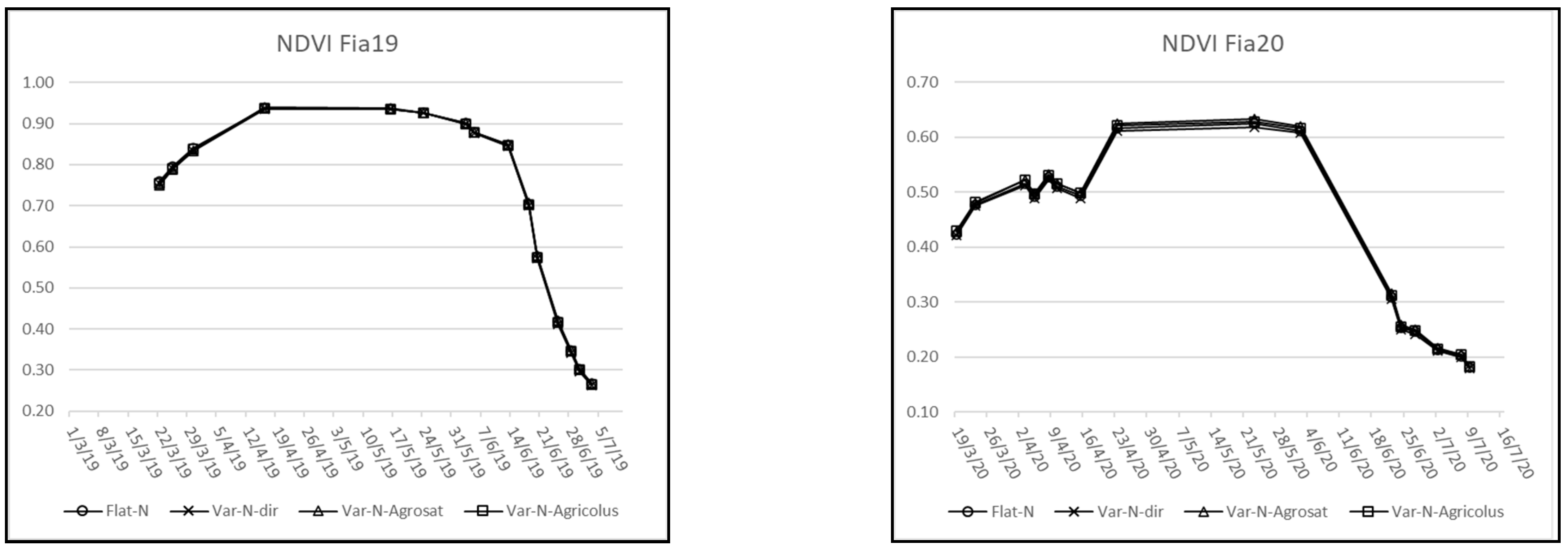
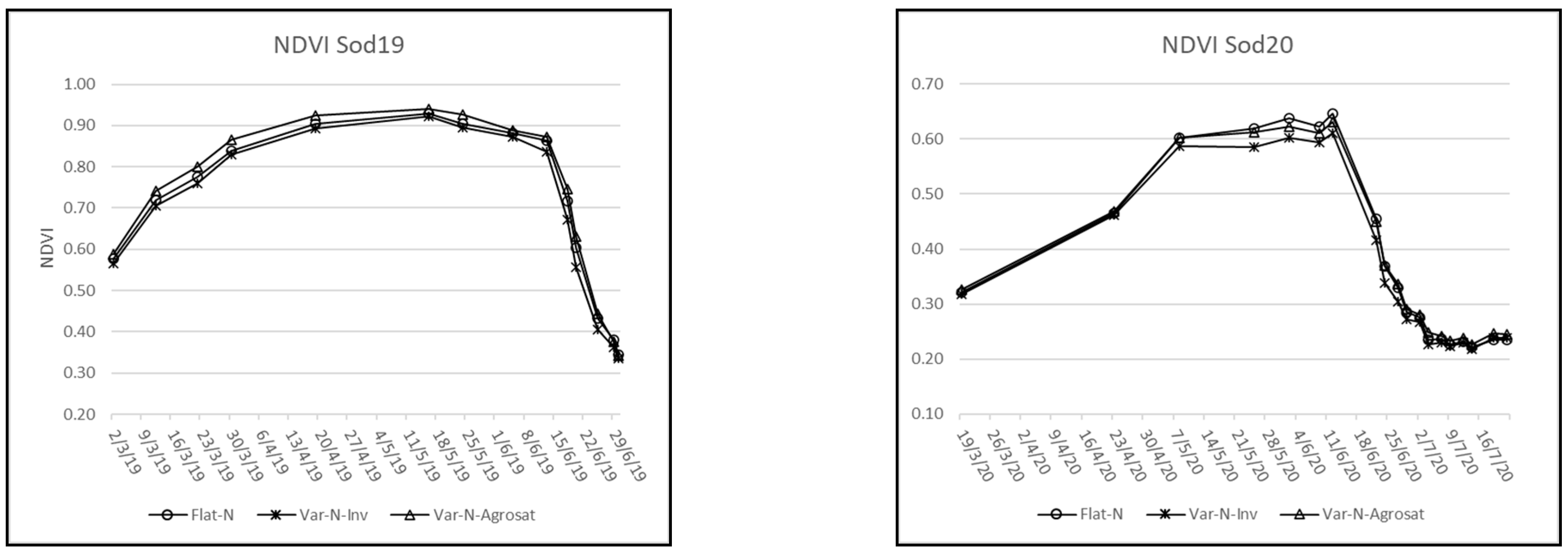
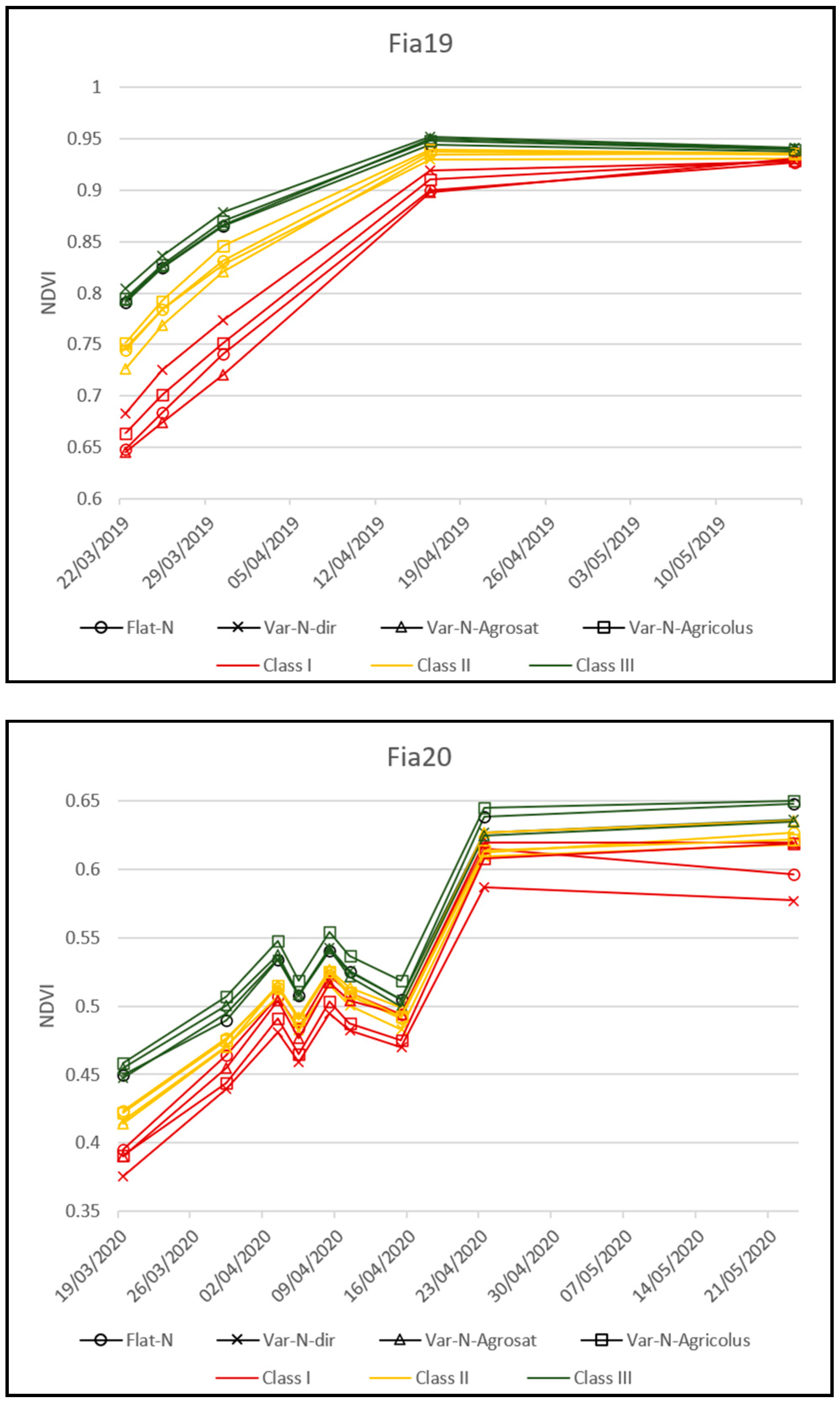
2.5. NDVI Seasonal Trend

All of the level-2A Sentinel-2 images with no cloud cover on the study areas were collected from the second fertilization to the harvest, in order to monitor and compare the NDVI of experimental treatments (15 images for Fia19, 16 images for Fia20, 13 for Sod19, 19 for Sod20). Average NDVI values were calculated for each experimental unit using the SAGA “raster statistics for polygons” tool included in the QGIS processing framework. This tool allows the user to calculate statistics about raster cell values contained in zones defined by a vector layer of polygons.
Another analysis was performed by classifying plots according to three classes, defined by dividing the NDVI range revealed by the S2 image acquired before the second fertilization into three equal parts. In addition, total nitrogen distribution and yield data were retrieved and compared for each of these groupings.
A final Pearson correlation analysis between the NDVI data and the soil variables (for Fia fields) and yield variables (for Fia and Sod fields) was developed in order to explore the possibility of predicting these variables using this vegetation index.

2.6. Grain Yield

For Fia19, the harvest was carried out on 12 and 14 July 2019, and for Fia20 on 9 July 2020, using a Claas Lexion 630 combine harvester equipped with an automatic guide device connected to the regional RTK network and a Topcon YieldTrakk system (based on grain mass flow and moisture sensors). After the input of the specific grain weight by the operator, the system produced a georeferenced yield map for the whole field as an ESRI polygon shapefile. The resulting polygons’ size depends on the feed rate, the collected mass, and the cutter bar’s working width (in this case, 7 m). The system also corrects the base width of the polygons when the combine passes over already collected field portions.
A data cleaning technique was applied to yield data according to the following steps: (1) all values outside the general average ± 2.5 * standard deviation range were eliminated, statistically considered outliers [70]; (2) all values collected close to the drainage system were eliminated—this is because the system in those areas records the entire cutter bar as operational, while the portion above the drainage system does not collect anything; and (3) all values falling in the 10 m portion before and after the experimental units’ transitions were eliminated, in order to avoid the values of one experimental unit being counted in the adjacent one due to the delay time. The delay time of the yield tracking system is the time required for the harvested grain to reach the reading sensor positioned on the hopper. This parameter is necessary in order to associate the harvested product with the correct geographical position instead of the position in which the combine is when the product reaches the reading sensor. The system sets the default delay time to 9 seconds, but the actual delay time between harvesting and reading depends on many factors, including threshing rotation speed, crop density, the state of maturation, and the moisture content of the wheat [71]. The resulting cleaned data were intersected with the experimental units in order to calculate the average yield expressed in Mg ha−1, which was used for the comparative analysis between treatments.
For the Sod fields, the harvest, carried out on 8 July 2019 and 23 July 2020, was performed by collecting and weighing each experimental unit’s yield. Although very time-consuming, this procedure provided very accurate yield data for each experimental unit and treatment. For Sod19, the experimental unit “1” (Var-N-Dir) was successively excluded from the experiment due to water stagnation located in that area, which compromised the normal comparison conditions.

2.7. Protein Content

For all fields, grain sampling was performed a few days before harvest in order to determine the grain protein content (Fia19: 27 June 2019; Fia20: 9 July 2020; Sod19: 26 June 2019; Sod20: 10 July 2020). For Fia19 and Fia20, a sample from each experimental unit was collected, for a total of 52 samples and 60 samples, respectively. For Sod19, 2 samples per experimental unit were collected (considering their wider area), for a total of 24 samples, while for Sod20, a sample per experimental unit was collected, for a total of 18 samples. Each sample was made up of four elementary subsamples randomly taken in the plot. All samples were analyzed according to the official Kjeldahl method [57].

2.8. Statistical Analysis

The inferential statistical analysis in this study was conducted separately for the four fields, considering them as independent experiments. All analyses were conducted considering the mean values of the variables calculated for each experimental unit. The analysis of variance (ANOVA) and Tukey’s HSD test (0.05 level of significance) were performed for the main variables in order to test the significance of differences between the treatments within each field. Pearson correlation was carried out in order to test the correlation between selected variables. All of the statistical analysis was performed using the statistics software R [72] (Version 4.0.3) and the “agricolae” package [73] (Version 1.3.3).

3. Results

The seasonal trend of crop NDVI variation for all treatments in each of the four fields is reported in Figure 4. Differences among treatments in NDVI values (average at field scale) were practically null in Fia fields and little in Sod fields, despite the N supplied by the second N application differing by up to three rates of kg N ha−1 (Table 5). Instead, the interannual difference was macroscopic in terms of within-crop-season trends and peak values.
As far as grain yield is concerned, differences were always very little and never significant (p-value > 0.10) (Table 6, Figure 5). Consequently, based on the N supplied by the second N application, the NUE (nitrogen use efficiency—derived from the ratio between kg of harvested grain and kg of nitrogen input) was higher the lower the N supplied. Var-N-inv and Var-N-dir showed the highest NUE (p-value < 0.05), followed by Var-N-Agricolus and then by Flat-N and Var-N-Agrosat, which did not differ substantially. The high variability in Var-N-Agricolus for Fia19 accounted for the lack of significant differences between Var-N-Agrosat and Flat-N. No significant differences were recorded for protein content, whose range for all treatments within the same field was in the order of 0.5% or less.
For Fia19, the NDVI time series analysis was performed by classifying plots according to three NDVI classes (NDVI ≤ 0.70; 0.70 < NDVI ≤ 0.77; NDVI > 0.77), as revealed by the S2 image from 22 March 2019 (Table 7, Figure 6). For Fia20, the NDVI time series analysis was performed by classifying plots according to three NDVI classes (NDVI ≤ 0.40; 0.40 < NDVI ≤ 0.44; NDVI > 0.44), as revealed by the S2 image from 19 March 2020 (Table 7, Figure 6). The differences in terms of yield were not significant in either field, while for the Fia20 field, the May 23 NDVI values of Var-N-Agricolus and Var-N-Agrosat were significantly different from Var-N-dir, but not from Flat-N.

Correlation Analysis between NDVI, Yield, and Soil Data

The results of the Pearson correlation analysis between the NDVI data and soil variables (for Fia fields) and yield variables (for Fia and Sod fields) are reported in Table 8, Table 9, Table 10 and Table 11. The correlations are based on the mean values from the individual plots.
Our results indicate relevant correlations only in few cases. For Fia20, the NDVI showed a high correlation with the yield between the last weeks of May and 1 June. Moreover, other fields showed an increase in correlation during the same period, which dropped quickly after that—except for Fia19, which showed a shifted peak towards mid-June.
Concerning grain protein content, for the 2018/19 season, there seems to be a correlation peak for both fields in the period around the end of March, and a subsequent second peak, with Fia19 reaching a correlation of 0.4 in early June and Sod19 reaching a peak of 0.8 between the second and third weeks of June. Fia20 shows its peak towards the last week of May, with a high average correlation with the NDVI of the whole season, while Sod20 starts out having a negative correlation for the whole first part of the season, becoming positive from June onwards.
For Fia19 and Fia20, a Pearson correlation index between grain yield and the soil parameters (clay, organic matter, and total nitrogen content) was also explored. A significative inverse correlation between yield and organic matter was found in the Fia19field.

4. Discussion

Our results show a substantial difference at the field scale, mainly linked to the different climatic conditions in the two cropping years, with respect to the effects of the different fertilization approaches. Our results show that a “Var” approach with a lower overall N rate (Var-N-inv, Var-N-dir, Var-N-Agricolus) gave the same grain yield with lower N input in all fields (Table 6). In fact, the NUE calculated with respect to the grain yield was significantly (p-value < 0.05) higher compared to Flat-N, Var-N-Agrosat, and Var-N-Agricolus in all cases. This result is consistent with the work of Raun et al. [74], who reported that the VRT method improved the NUE (nitrogen use efficiency) by 15% compared to a flat rate. The results are also consistent with the work of Vizzari et al. [6], who reported no decrease in grain yield using “Var” approaches while reducing the rate by about 20 kg N ha−1. This evidence is economically and environmentally relevant, since the surplus N would involve luxury consumption or leaching risks, depending on whether or not it would be absorbed by the wheat’s roots. Thanks to the optimal climatic conditions of the 2018–2019 cropping season, it is evident that even the most conservative approach in terms of nitrogen intake worked in saturation conditions anyway. Moreover, an increase in grain quality may not be advocated to justify the N surplus, since the increase in the grain protein content of the flat-N and Var-N-Agrosat treatments was negligible and never significant.
The lack of relevant average differences in grain yield among treatments is in line with the NDVI values recorded after the second N application, since the differences in NDVI between treatments were either null (2019) or tiny and non-critical (2020). This occurrence may happen, especially for high NDVI values [26], when other variables aside from N nutritional status come into play, such as the soil’s hydrological properties [31,75] or the rainfall regime.
In this regard, both experimental years were abnormal. The first was exceptionally rainy, and the second exceptionally dry, which masked the N treatments’ effect. Thus, for example, the negative correlation found between grain yield and the clay and organic matter content of the soil in the 2018–2019 season was likely independent of the soil’s nutrient content, being more likely due to soil water saturation caused by the abundant rainfall. On the other hand, in the 2019–2020 season, the rainfall in winter and spring was so scarce that the wheat growth (after shoot elongation) and the grain filling were limited by water rather than N availability. The small gradient in clay content could not have counteracted the severe water deficiency. Interestingly, in this year, both the grain protein content and the yield were lower than in the previous year. This result was unexpected since, normally, when the crop is well N-fed (as it was in our case), biomass production is inversely correlated to the concentration of N compounds—including protein production [76]. In this regard, we can only speculate that the very low water availability of 2020 somehow impaired N absorption or relocation to grains [77].
Regarding the correlation between yield and NDVI (Table 8 and Table 9), the strong correlation observed in the Fia20 field could be related to the unfavorable season, which did not cause typical NDVI saturation. Consequently, the intra-field heterogeneity was indicative of the crop’s phenological growth and the LAI, which was reflected in the final yield. Sod19 and Sod20 showed correlation peaks in the same period as Fia20, but with a lower Pearson value of around 0.4. This can be explained by the fact that the experimental units in these fields were very large compared to the NDVI gradient, and with a higher yield data resolution, the correlation would likely have been stronger. These results are in line with the literature, where the existence of a correlation between NDVI and yield is widely reported [22,37,78]. Fia19 showed a low correlation between NDVI and grain yield, in contrast to other fields and most of the relevant literature. This result could be explained by the optimal conditions of the season 2018–19 having translated into high crop vigor, resulting in a low intra-field variability and, above all, a saturation of the NDVI, no longer able to detect the differences in vigor above a certain threshold. This flattening of the variability could result in the low correlation found with the yield data.
Regarding the correlations between protein content and NDVI (Table 10 and Table 11), although in this case the correlations are on average high for all fields, it is difficult to find a causality that explains these data, starting with the Sod20 field which, in contrast to all of the others, seems to show a negative correlation with NDVI. The significative inverse correlation between yield and organic matter in the Fia19 field is atypical, and in contrast to literature, but could be explained due to the overlapping of the clay and organic matter spatial trends along the field. The strong clayey character of the soil can cause compaction, with negative consequences on yield [79].
Any evaluation on the suitability of different Var-N- approaches (i.e., -dir, -inv, -Agrosat, -Agricolus) appears meaningless if not linked to the climatic conditions characterizing the cropping seasons and to a careful evaluation of the initial and final conditions in terms of NDVI and final yield. During the first cropping season, the optimal climatic conditions meant that reducing the overall N rate (i.e., Var-N-dir, Var-N-inv, Var-N-Agricolus) was the most suitable strategy for increasing the nitrogen use efficiency without compromising grain yield and quality. Conversely, during the second cropping season, a direct approach (Var-N-dir) did not lead to the same results. In fact, interesting evidence in support of this conclusion could be found in the most disadvantaged areas of the Fia20 field; what emerges is that, when the crop season is unfavorable, well-studied management may make the difference in limiting N losses. Analyzing the NDVI class “I” (including all of the field pixels with an NDVI value ≤ 0.40 on 19 March 2020), it emerges that, even if the differences are slight and not statistically significant in terms of yield, and additional experiments would be necessary, the advanced model strategies (Var-N-Agricolus and Var-N-Agrosat) seem to give the best results both in terms of NDVI (Figure 6, bottom) and in terms of yield (Table 7), also resulting in a more spatial homogeneous production across the field. Of the two advanced models, Agricolus resulted in the highest NUE (Table 6). The probable reading of this result is that a full nitrogen dose was not the best choice for that year and that area, because the crop could not exploit it given the weather and climatic limits. At the same time, limiting the nitrogen rate to a minimum with a direct approach did not turn out to be a good strategy, because the crop would have been able to exploit a slightly higher dose, even if not the maximum.

5. Conclusions

Our study, carried out in two fields and two cropping seasons, investigated the differences between a flat N fertilization rate and four variable rates defined through simplified and complex methods, based on Sentinel-2 NDVI, applied to define the second fertilization. Three of the four variable rates were aimed at reducing the overall N input (Var-N-inv, Var-N-dir, and Var-N-Agricolus), while he other was aimed at maintaining the same overall input (Var-N-Agrosat) as in the flat rate (Flat-N) while optimizing the N fertilization according to the supposed N requirement as revealed by the NDVI data.
Our results show that the variable approaches with lower overall N rates (Var-N-inv, Var-N-dir, and Var-N-Agricolus) gave the same grain yield as the others (flat-N, Var-N-Agosat) while obtaining a higher NUE. However, the various approaches can be correctly evaluated only when contextualized to the respective climatic season. In fact, the strong effect of the opposite climatic trend across the two seasons is an explicit confirmation that weather is the main factor influencing the yield of a rainfed crop, followed by soil texture, which typically influences the vigor gradient of the crop. This evidence suggests that VRT nitrogen fertilization may only partially mitigate the heterogeneity of production determined by such environmental factors.
In general, in favorable seasons, a low-input nitrogen fertilization driven by the NDVI direct model (Var-N-dir) may be the best choice in contexts where the vigor crop gradient is a direct reflection of the soil gradient. This approach provides nitrogen where the crop can use it and saves it where the crop is limited by other factors, limiting leaching in deep water, preserving the environment, and saving money. On the other hand, in unfavorable seasons, when decision support could be more helpful, the more advanced data-driven models (Agricolus and AgroSat) may be more effective in limiting losses and maintaining more homogeneous intra-field production. This evidence takes on greater importance for rainfed wheat given the increasing frequency of anomalous climate phenomena.

Author Contributions

Conceptualization, M.V., F.S.S. and P.B.; methodology F.S.S., P.B., M.V., P.T., S.A. and E.R.; investigation, F.S.S.; data curation, F.S.S., P.T., S.A. and E.R.; writing—original draft preparation, F.S.S., P.B. and M.V.; writing—review and editing, P.B., M.V., F.S.S., P.T., E.R. and S.A.; visualization, F.S.S.; supervision, M.V. and P.B.; project administration, M.V. All authors have read and agreed to the published version of the manuscript.

Funding

This research was developed within the framework of the project “RTK 2.0—Prototyping an RTK Network and Innovative Technological Applications for Agricultural Processes Automation and Precision Farming Information”—Rural Development Programme 2014–2020 of Umbria Region—Meas. 16.1—App. 84250020256.

Institutional Review Board Statement

Not applicable.

Informed Consent Statement

Not applicable.

Data Availability Statement

Data are available, upon any reasonable request, from the authors.

Acknowledgments

The authors wish to thank Mauro Brunetti of the “Fondazione per l’Istruzione Agraria” farm, Giuseppe Baldelli and Simone Falcini of the “Sodalizio di San Martino” farm, the staff of the “Francesco Di Camillo” company, and Daniele Luchetti of the FIELDLAB of the Department of Agricultural, Food, and Environmental Sciences, University of Perugia for their constructive and valuable support during the experimental stages of the research.

Conflicts of Interest

The authors declare no conflict of interest.

References

  1. Aydinalp, C.; Cresser, M.S. The Effects of Global Climate Change on Agriculture. Am. J. Agric. Environ. Sci. 2008, 3, 672–676. [Google Scholar]
  2. Odegard, I.; Van Der Voet, E. The future of food—Scenarios and the effect on natural resource use in agriculture in 2050. Ecol. Econ. 2014, 97, 51–59. [Google Scholar] [CrossRef]
  3. Pierce, F.J.; Nowak, P. Aspects of Precision Agriculture. Adv. Agron. 1999, 67, 1–85. [Google Scholar] [CrossRef]
  4. Zheng, Q.; Huang, W.; Cui, X.; Shi, Y.; Liu, L. New Spectral Index for Detecting Wheat Yellow Rust Using Sentinel-2 Multispectral Imagery. Sensors 2018, 18, 868. [Google Scholar] [CrossRef] [PubMed] [Green Version]
  5. Drusch, M.; Del Bello, U.; Carlier, S.; Colin, O.; Fernandez, V.; Gascon, F.; Hoersch, B.; Isola, C.; Laberinti, P.; Martimort, P.; et al. Sentinel-2: ESA’s Optical High-Resolution Mission for GMES Operational Services. Remote Sens. Environ. 2012, 120, 25–36. [Google Scholar] [CrossRef]
  6. Segarra, J.; Buchaillot, M.L.; Araus, J.L.; Kefauver, S.C. Remote sensing for precision agriculture: Sentinel-2 improved features and applications. Agronomy 2020, 10, 641. [Google Scholar] [CrossRef]
  7. Delloye, C.; Weiss, M.; Defourny, P. Retrieval of the canopy chlorophyll content from Sentinel-2 spectral bands to estimate nitrogen uptake in intensive winter wheat cropping systems. Remote Sens. Environ. 2018, 216, 245–261. [Google Scholar] [CrossRef]
  8. Copernicus Open Access Hub. Available online: https://scihub.copernicus.eu/ (accessed on 28 May 2021).
  9. Clevers, J.G.P.W.; Kooistra, L.; van den Brande, M.M.M. Using Sentinel-2 data for retrieving LAI and leaf and canopy chlorophyll content of a potato crop. Remote Sens. 2017, 9, 405. [Google Scholar] [CrossRef] [Green Version]
  10. Silleos, N.G.; Alexandridis, T.; Gitas, I.Z.; Perakis, K. Vegetation Indices: Advances Made in Biomass Estimation and Vegetation Monitoring in the Last 30 Years. Geocarto Int. 2006, 21, 21–28. [Google Scholar] [CrossRef]
  11. Xue, J.; Su, B. Significant Remote Sensing Vegetation Indices: A Review of Developments and Applications. J. Sens. 2017, 2017, 1–17. [Google Scholar] [CrossRef] [Green Version]
  12. Messina, G.; Peña, J.; Vizzari, M.; Modica, G. A Comparison of UAV and Satellites Multispectral Imagery in Monitoring Onion Crop. An Application in the ‘Cipolla Rossa di Tropea’ (Italy). Remote Sens. 2020, 12, 3424. [Google Scholar] [CrossRef]
  13. Tassi, A.; Vizzari, M. Object-Oriented LULC Classification in Google Earth Learning Algorithms. Remote Sens. 2020, 2020, 3776. [Google Scholar] [CrossRef]
  14. Rouse, J.W.; Hass, R.H.; Schell, J.A.; Deering, D.W. Monitoring vegetation systems in the great plains with ERTS. In Proceedings of the 3rd ERTS Symposium, NASA SP-351, Washington, DC, USA, 10–14 December 1973. [Google Scholar]
  15. Muñoz-Huerta, R.F.; Guevara-Gonzalez, R.G.; Contreras-Medina, L.M.; Torres-Pacheco, I.; Prado-Olivarez, J.; Ocampo-Velazquez, R.V. A Review of Methods for Sensing the Nitrogen Status in Plants: Advantages, Disadvantages and Recent Advances. Sensors 2013, 13, 10823–10843. [Google Scholar] [CrossRef]
  16. Cabrera-Bosquet, L.; Molero, G.; Stellacci, A.; Bort, J.; Nogués, S.; Araus, J. NDVI as a potential tool for predicting biomass, plant nitrogen content and growth in wheat genotypes subjected to different water and nitrogen conditions. Cereal Res. Commun. 2011, 39, 147–159. [Google Scholar] [CrossRef]
  17. Carlson, T.N.; Ripley, D.A. On the relation between NDVI, fractional vegetation cover, and leaf area index. Remote Sens. Environ. 1997, 62, 241–252. [Google Scholar] [CrossRef]
  18. Stamatiadis, S.; Christofides, C.; Tsadilas, C.; Samaras, V.; Schepers, J.S.; Francis, D. Ground-Sensor Soil Reflectance as Related to Soil Properties and Crop Response in a Cotton Field. Precis. Agric. 2005, 6, 399–411. [Google Scholar] [CrossRef]
  19. Hansen, P.; Schjoerring, J. Reflectance measurement of canopy biomass and nitrogen status in wheat crops using normalized difference vegetation indices and partial least squares regression. Remote Sens. Environ. 2003, 86, 542–553. [Google Scholar] [CrossRef]
  20. Magney, T.; Eitel, J.U.; Huggins, D.R.; Vierling, L.A. Proximal NDVI derived phenology improves in-season predictions of wheat quantity and quality. Agric. For. Meteorol. 2016, 217, 46–60. [Google Scholar] [CrossRef]
  21. Herrmann, I.; Pimstein, A.; Karnieli, A.; Cohen, Y.; Alchanatis, V.; Bonfil, D. LAI assessment of wheat and potato crops by VENμS and Sentinel-2 bands. Remote Sens. Environ. 2011, 115, 2141–2151. [Google Scholar] [CrossRef]
  22. Sultana, S.R.; Ali, A.; Ahmad, A.; Mubeen, M.; Zia-Ul-Haq, M.; Ahmad, S.; Ercisli, S.; Jaafar, H.Z.E. Normalized Difference Vegetation Index as a Tool for Wheat Yield Estimation: A Case Study from Faisalabad, Pakistan. Sci. World J. 2014, 2014, 1–8. [Google Scholar] [CrossRef] [Green Version]
  23. Zhu, Y.; Yao, X.; Tian, Y.; Liu, X.; Cao, W. Analysis of common canopy vegetation indices for indicating leaf nitrogen accumulations in wheat and rice. Int. J. Appl. Earth Obs. Geoinf. 2008, 10, 1–10. [Google Scholar] [CrossRef]
  24. Cao, Q.; Miao, Y.; Feng, G.; Gao, X.; Li, F.; Liu, B.; Yue, S.; Cheng, S.; Ustin, S.L.; Khosla, R. Active canopy sensing of winter wheat nitrogen status: An evaluation of two sensor systems. Comput. Electron. Agric. 2015, 112, 54–67. [Google Scholar] [CrossRef]
  25. Tosti, G.; Farneselli, M.; Benincasa, P.; Guiducci, M. Nitrogen Fertilization Strategies for Organic Wheat Production: Crop Yield and Nitrate Leaching. Agron. J. 2016, 108, 770–781. [Google Scholar] [CrossRef] [Green Version]
  26. Benincasa, P.; Antognelli, S.; Brunetti, L.; Fabbri, C.A.; Natale, A.; Sartoretti, V.; Modeo, G.; Guiducci, M.; Tei, F.; Vizzari, M. Reliability of NDVI derived by high resolution satellite and UAV compared to in-field methods for the evaluation of early crop n status and grain yield in wheat. Exp. Agric. 2018, 54, 604–622. [Google Scholar] [CrossRef]
  27. Spiertz, J.H.J. Nitrogen, sustainable agriculture and food security. A review. Agron. Sustain. Dev. 2010, 30, 43–55. [Google Scholar] [CrossRef] [Green Version]
  28. Vizzari, M.; Antognelli, S.; Pauselli, M.; Benincasa, P.; Farneselli, M.; Morbidini, L.; Borghi, P.; Bodo, G.; Santucci, A. Potential Nitrogen Load from Crop-Livestock Systems. Int. J. Agric. Environ. Inf. Syst. 2016, 7, 21–40. [Google Scholar] [CrossRef] [Green Version]
  29. Vizzari, M.; Santucci, A.; Casagrande, L.; Pauselli, M.; Benincasa, P.; Farneselli, M.; Antognelli, S.; Morbidini, L.; Borghi, P.; Bodo, G. Potential Nitrogen Load from Crop-Livestock Systems: An Agri-Environmental Spatial Database for a Multi-Scale Assessment; Springer: Berlin/Heidelberg, Germany, 2015. [Google Scholar]
  30. Bourdin, F.; Morell, F.; Combemale, D.; Clastre, P.; Guérif, M.; Chanzy, A. A tool based on remotely sensed LAI, yield maps and a crop model to recommend variable rate nitrogen fertilization for wheat. Adv. Anim. Biosci. 2017, 8, 672–677. [Google Scholar] [CrossRef]
  31. Basso, B.; Ritchie, J.T.; Cammarano, D.; Sartori, L. A strategic and tactical management approach to select optimal N fertilizer rates for wheat in a spatially variable field. Eur. J. Agron. 2011, 35, 215–222. [Google Scholar] [CrossRef]
  32. Diacono, M.; Rubino, P.; Montemurro, F. Precision nitrogen management of wheat. A review. Agron. Sustain. Dev. 2013, 33, 219–241. [Google Scholar] [CrossRef]
  33. Song, X.; Wang, J.; Huang, W.; Liu, L.; Yan, G.; Pu, R. The delineation of agricultural management zones with high resolution remotely sensed data. Precis. Agric. 2009, 10, 471–487. [Google Scholar] [CrossRef]
  34. CropSAT. Available online: https://cropsat.com/ (accessed on 12 May 2021).
  35. AgroSat. Available online: https://www.agrosat.it (accessed on 12 May 2021).
  36. OneSoil. Available online: https://onesoil.ai/en/ (accessed on 12 May 2021).
  37. Toscano, P.; Castrignanò, A.; Di Gennaro, S.F.; Vonella, A.V.; Ventrella, D.; Matese, A. A Precision Agriculture Approach for Durum Wheat Yield Assessment Using Remote Sensing Data and Yield Mapping. Agronomy 2019, 9, 437. [Google Scholar] [CrossRef] [Green Version]
  38. Toscano, P.; Ranieri, R.; Matese, A.; Vaccari, F.; Gioli, B.; Zaldei, A.; Silvestri, M.; Ronchi, C.; La Cava, P.; Porter, J.; et al. Durum wheat modeling: The Delphi system, 11 years of observations in Italy. Eur. J. Agron. 2012, 43, 108–118. [Google Scholar] [CrossRef]
  39. Ambrosone, M.; Matese, A.; Di Gennaro, S.F.; Gioli, B.; Tudoroiu, M.; Genesio, L.; Miglietta, F.; Baronti, S.; Maienza, A.; Ungaro, F.; et al. Retrieving soil moisture in rainfed and irrigated fields using Sentinel-2 observations and a modified OPTRAM approach. Int. J. Appl. Earth Obs. Geoinf. 2020, 89, 102113. [Google Scholar] [CrossRef]
  40. Magno, R.; Rocchi, L.; Dainelli, R.; Matese, A.; Di Gennaro, S.; Chen, C.-F.; Son, N.-T.; Toscano, P. AgroShadow: A New Sentinel-2 Cloud Shadow Detection Tool for Precision Agriculture. Remote Sens. 2021, 13, 1219. [Google Scholar] [CrossRef]
  41. Cisternino, A.; Incrocci, L.; Lulli, L.; Mariotti, M.; Masoni, A.; Massa, D.; Massai, R.; Pardossi, A.; Remorini, D. Redazione del Piano di Concimazione; Felici Editore: Ghezzano, Italy, 2010. [Google Scholar]
  42. Nawar, S.; Corstanje, R.; Halcro, G.; Mulla, D.; Mouazen, A.M. Delineation of Soil Management Zones for Variable-Rate Fertilization, 1st ed.; Elsevier: Amsterdam, The Netherlands, 2017. [Google Scholar]
  43. Zhang, N.; Wang, M.; Wang, N. Precision agriculture—A worldwide overview. In Computers and Electronics in Agriculture; ScienceDirect: Amsterdam, The Netherlands, 2002; pp. 113–132. [Google Scholar]
  44. Sharipov, G.M.; Heiß, A.; Eshkabilov, S.L.; Griepentrog, H.W.; Paraforos, D.S. Variable rate application accuracy of a centrifugal disc spreader using ISO 11783 communication data and granule motion modeling. Comput. Electron. Agric. 2021, 182, 106006. [Google Scholar] [CrossRef]
  45. Ross, K.W.; Morris, D.K.; Johannsen, C.J. A Review of Intra-Field Yield Estimation from Yield Monitor Data. Appl. Eng. Agric. 2008, 24, 309–317. [Google Scholar] [CrossRef]
  46. Arslan, S.; Colvin, T.S. Grain Yield Mapping: Yield Sensing, Yield Reconstruction, and Errors. Precis. Agric. 2002, 3, 135–154. [Google Scholar] [CrossRef]
  47. Leroux, C.; Jones, H.; Clenet, A.; Dreux, B.; Becu, M.; Tisseyre, B. A general method to filter out defective spatial observations from yield mapping datasets. Precis. Agric. 2018, 19, 789–808. [Google Scholar] [CrossRef]
  48. Vizzari, M.; Santaga, F.; Benincasa, P. Sentinel 2-Based Nitrogen VRT Fertilization in Wheat: Comparison between Traditional and Simple Precision Practices. Agronomy 2019, 9, 278. [Google Scholar] [CrossRef] [Green Version]
  49. Santaga, F.; Benincasa, P.; Vizzari, M. Using Sentinel 2 Data to Guide Nitrogen Fertilization in Central Italy: Comparison Between Flat, Low VRT and High VRT Rates Application in Wheat; Springer: Berlin/Heidelberg, Germany, 2020; pp. 78–89. [Google Scholar]
  50. PR22R58. Available online: https://www.corteva.it/prodotti-e-soluzioni/sementi/frumento/PR22R58.html (accessed on 10 May 2021).
  51. Oregrain. Available online: https://ragt-sementi.it/it-it/nos-varietes/oregrain-grano-tenero (accessed on 10 May 2021).
  52. Rebelde. Available online: https://www.apsovsementi.com/it/portfolio/rebelde/ (accessed on 10 May 2021).
  53. Bandera. Available online: https://ragt-sementi.it/it-it/nos-varietes/bandera-grano-tenero (accessed on 10 May 2021).
  54. Bandera. Available online: http://apuliasemi.it/wp/portfolio/bandera/ (accessed on 10 May 2021).
  55. Indorante, S.J.; Hammer, R.D.; Koenig, P.G.; Follmer, L.R. Particle-Size Analysis by a Modified Pipette Procedure. Soil Sci. Soc. Am. J. 1990, 54, 560–563. [Google Scholar] [CrossRef]
  56. Soltner, D. Le Bases de la Production Vegetale, 16th ed.; Tecniques, Collection Sciences et Agricoles: Sainte Gemmes Sur Loire, France, 1988. [Google Scholar]
  57. Zumbado, H.; Lutz, A. A Guide to Kjeldahl Nitrogen Determination Methods and Apparatus; ExpotechUSA: Houston, TX, USA, 1998. [Google Scholar]
  58. QGIS Development Team. QGIS Geographic Information System. Open Source Geospatial Foundation Project. 2020. Available online: http://qgis.osgeo.org (accessed on 4 June 2021).
  59. Soil Conservation Service. Soil Taxonomy: A Basic System of Soil Classification for Making and Interpreting Soil Surveys; Natural Resources Conservation Service: Washington, DC, USA, 1975. [Google Scholar]
  60. Beck, H.E.; Zimmermann, N.E.; McVicar, T.; Vergopolan, N.; Berg, A.; Wood, E.F. Present and future Köppen-Geiger climate classification maps at 1-km resolution. Sci. Data 2018, 5, 180214. [Google Scholar] [CrossRef] [Green Version]
  61. Sowers, K.E.; Pan, W.L.; Miller, B.C.; Smith, J.L. Nitrogen Use Efficiency of Split Nitrogen Applications in Soft White Winter Wheat. Agron. J. 1907, 86, 942–948. [Google Scholar] [CrossRef]
  62. López-Bellido, R.; López-Bellido, L. Efficiency of nitrogen in wheat under Mediterranean conditions: Effect of tillage, crop rotation and N fertilization. Field Crop Res. 2001, 71, 31–46. [Google Scholar] [CrossRef]
  63. López-Bellido, L.; López-Bellido, R.J.; Redondo, R. Nitrogen efficiency in wheat under rainfed Mediterranean conditions as affected by split nitrogen application. Field Crop Res. 2005, 94, 86–97. [Google Scholar] [CrossRef]
  64. Vian, A.L.; Bredemeier, C.; Turra, M.A.; Giordano, C.P.D.S.; Fochesatto, E.; Da Silva, J.A.; Drum, M.A. Nitrogen management in wheat based on the normalized difference vegetation index (NDVI). Ciênc. Rural 2018, 48. [Google Scholar] [CrossRef]
  65. Di Gennaro, S.F.; Rizza, F.; Badeck, F.W.; Berton, A.; Delbono, S.; Gioli, B.; Toscano, P.; Zaldei, A.; Matese, A. UAV-based high-throughput phenotyping to discriminate barley vigour with visible and near-infrared vegetation indices. Int. J. Remote Sens. 2017, 39, 5330–5344. [Google Scholar] [CrossRef]
  66. Casa, R.; Castaldi, F.; Pascucci, S.; Pignatti, S. Chlorophyll estimation in field crops: An assessment of handheld leaf meters and spectral reflectance measurements. J. Agric. Sci. 2014, 153, 876–890. [Google Scholar] [CrossRef]
  67. Maresma, Á.; Ariza, M.; Martínez, E.; Lloveras, J.; Martínez-Casasnovas, J.A. Analysis of Vegetation Indices to Determine Nitrogen Application and Yield Prediction in Maize (Zea mays L.) from a Standard UAV Service. Remote Sens. 2016, 8, 973. [Google Scholar] [CrossRef] [Green Version]
  68. Saberioon, M.M.; Gholizadeh, A. Novel approach for estimating nitrogen content in paddy fields using low altitude remote sensing system. ISPRS Int. Arch. Photogramm. Remote Sens. Spat. Inf. Sci. 2016, XLI-B1, 1011–1015. [Google Scholar] [CrossRef] [Green Version]
  69. Clevers, J.; Gitelson, A. Remote estimation of crop and grass chlorophyll and nitrogen content using red-edge bands on Sentinel-2 and -3. Int. J. Appl. Earth Obs. Geoinf. 2013, 23, 344–351. [Google Scholar] [CrossRef]
  70. Vega, A.; Córdoba, M.; Castro-Franco, M.; Balzarini, M. Protocol for automating error removal from yield maps. Precis. Agric. 2019, 20, 1030–1044. [Google Scholar] [CrossRef]
  71. Chung, S.-O.; Sudduth, K.A.; Drummond, S.T. Determining yield monitoring system delay time with geostatistical and data segmentation approaches. Trans. ASAE 2002, 45, 915–926. [Google Scholar] [CrossRef] [Green Version]
  72. R Core Team. R: A Language and Environment for Statistical Computing; R Foundation for Statistical Computing: Vienna, Austria, 2016. [Google Scholar]
  73. De Mendiburu, F. Package Agricolae; R Foundation for Statistical Computing: Vienna, Austria, 2020. [Google Scholar]
  74. Raun, W.R.; Solie, J.B.; Johnson, G.V.; Stone, M.L.; Mullen, R.W.; Freeman, K.W.; Thomason, W.E.; Lukina, E.V. Improving Nitrogen Use Efficiency in Cereal Grain Production with Optical Sensing and Variable Rate Application. Agron. J. 2002, 94, 815–820. [Google Scholar] [CrossRef] [Green Version]
  75. Zhao, C.; Liu, L.; Wang, J.; Huang, W.; Song, X.; Li, C. Predicting grain protein content of winter wheat using remote sensing data based on nitrogen status and water stress. Int. J. Appl. Earth Obs. Geoinf. 2005, 7, 1–9. [Google Scholar] [CrossRef]
  76. Guiducci, M.; Tosti, G.; Falcinelli, B.; Benincasa, P. Sustainable management of nitrogen nutrition in winter wheat through temporary intercropping with legumes. Agron. Sustain. Dev. 2018, 38, 31. [Google Scholar] [CrossRef] [Green Version]
  77. Aggarwal, P.K.; Sinha, S.K. Effect of Water Stress on Grain Growth and Assimilate Partitioning in two Cultivars of Wheat Contrasting in their Yield Stability in a Drought-Environment. Ann. Bot. 1984, 53, 329–340. [Google Scholar] [CrossRef]
  78. Wang, L.; Tian, Y.; Yao, X.; Zhu, Y.; Cao, W. Predicting grain yield and protein content in wheat by fusing multi-sensor and multi-temporal remote-sensing images. Field Crop Res. 2014, 164, 178–188. [Google Scholar] [CrossRef]
  79. Voorhees, W.B. The Effect of Soil Compaction on Crop Yield. SAE Tech. Pap. Ser. 1986, 95, 1078–1084. [Google Scholar] [CrossRef]
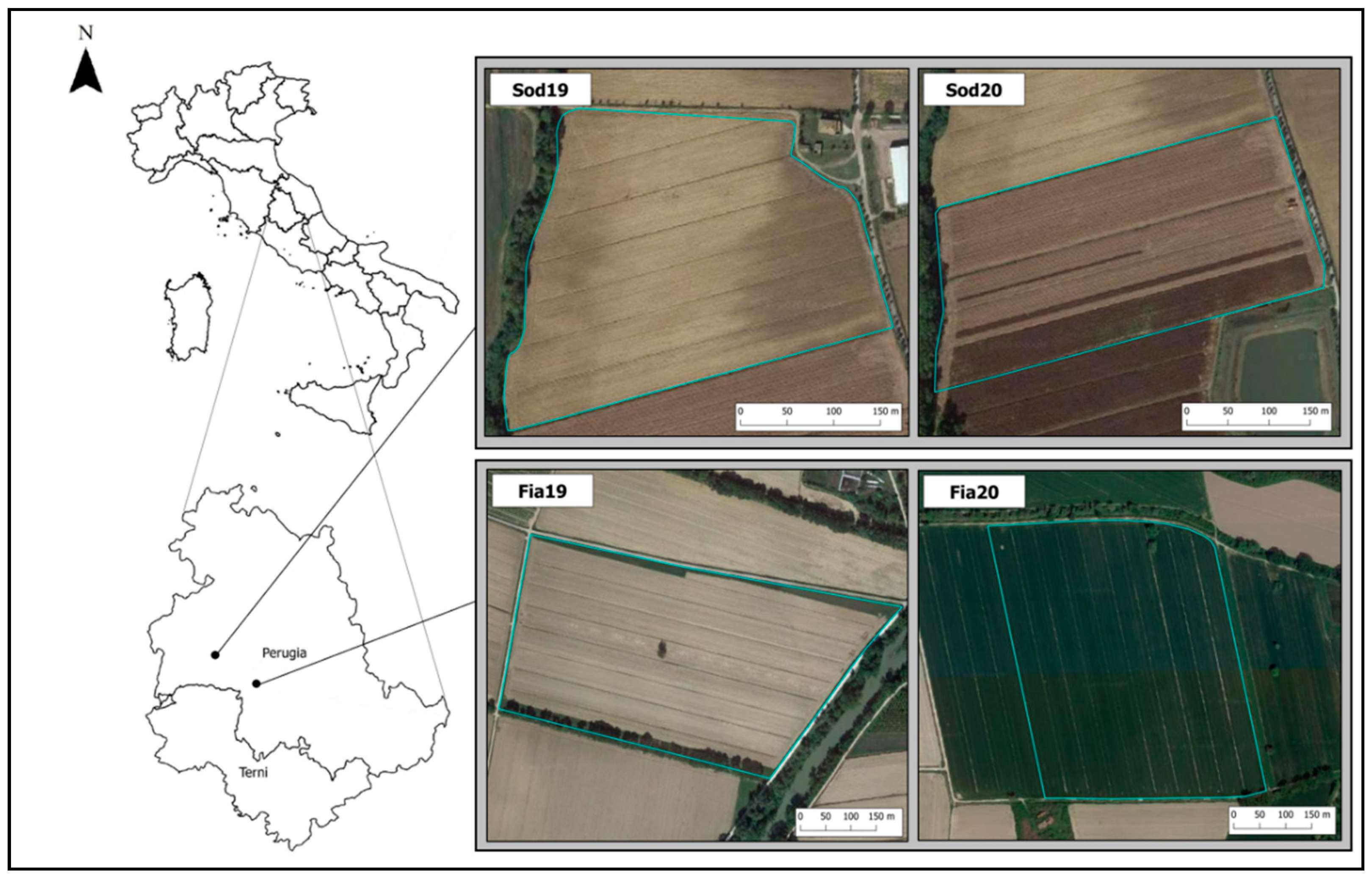
Figure 1. Geographical location of the study areas and experimental fields (outlined in cyan).
Agronomy 11 01156 g001
Figure 2. Monthly cumulated rainfall and average temperatures per decade during the wheat growing seasons (a) 2018–2019 and (b) 2019–2020 compared to the long-term mean values (temperature 1951–2018, rainfall 1921–2018).
Agronomy 11 01156 g002
Figure 3. Prescription maps (left) and NDVI calculated before the second fertilization (right) maps for Fia19, Fia20, Sod19, and Sod20 (top to bottom). The numbers on the plots indicate the different experimental treatments: Flat-N (1); Var-N-Inv (2); Var-N-Dir (3); Var-N-Agrosat (4); and Var-N-Agricolus (5). The fields’ outer borders are plotted in cyan.
Agronomy 11 01156 g003
Figure 4. NDVI seasonal trends of the five treatments in the four experimental fields.
Agronomy 11 01156 g004aAgronomy 11 01156 g004b
Figure 5. Top, from left to right: Fia19 and Fia20 yield maps used for quantitative analysis; bottom, from left to right: Sod19 and Sod20 yield quantities measured in each experimental unit. The numbers on the plots indicate the different experimental treatments: Flat-N (1); Var-N-Inv (2); Var-N-Dir (3); Var-N-Agrosat (4); and Var-N-Agricolus (5).
Agronomy 11 01156 g005
Figure 6. NDVI time series analysis, considering the three vigor classes (Class I: red lines; Class II: yellow lines; Class III: green lines) as identified in the S2 image from 22 March 2019 for Fia19 (top), and from 19 March 2020 for Fia20 (bottom).
Agronomy 11 01156 g006
Table 1. Location, coordinates, altimetry, extent, variety, sowing date, and previous crops of the experimental fields, as well as second N application date.
FieldFia19Fia20Sod19Sod20
LocationDeruta (PG),
Italy
Deruta (PG),
Italy
Mugnano (PG), ItalyMugnano (PG), Italy
Coordinates (WGS84)42°95′37″ N, 12°38′91″ E42°93′54″ N, 12°38′85″ E43°04′57″ N, 12°21′74″ E43°04′38″ N, 12°21′77″ E
Altimetry160 m ASL158 m ASL227 m ASL 227 m ASL
Extent (ha)20 ha20 ha10 ha9 ha
Previous CropMaize
(Zea mais L.)
Maize
(Zea mais L.)
Sunflower
(Helianthus annuus L.)
Maize
(Zea mais L.)
VarietyPR22R58OregrainRebeldeBandera
Sowing Date12 November 20186 December 2019 16 November 20187 January 2018
Second N Application Date25 March 201924 March 202018 March 20197 April 2020
Table 2. Wheat varieties used for the experimentation and their main characteristics, as provided by the seed companies.
VarietyPR22R58 [50]Oregrain [51]Rebelde [52]Bandera [53,54]
ClassificationBread wheatBread wheatStrength wheatBread wheat
Ripening CycleMedium–lateLateMediumEarly
Quantitative YieldVery highHighHighHigh
Etholithic WeightMediumMediumHighHigh
Grain Protein ContentMediumMedium–highVery highMedium
Table 3. Main soil sampling statistics for Fia19 and Fia20 fields.
FieldStatsMoisture
%
Sand
g/Kg
Silt
g/Kg
Clay
g/Kg
OM
g/Kg
N tot g/Kg
Fia19avg19.4%16.751.431.91.821.25
st.dev.1.38%7.684.076.150.2280.156
min14.4%5.339.224.61.410.95
max22.0%35.061.446.02.321.60
range7.6%29.722.221.40.910.65
Fia20avg19.8%27.146.126.81.460.99
st.dev.0.93%8.916.224.370.2030.088
min18.5%10.833.220.31.100.80
max21.8%46.057.135.02.191.20
range3.2%35.223.914.71.090.40
Table 4. Abbreviations and descriptions of the experimental treatments and the fields on which they were applied.
TreatmentDescriptionFields
Flat-NStandard rate calculated by a typical N balanceFia, Sod
Var-N-dirVariable rate calculated using a simplified linear model, adopting a proportional strategy (NDVI directly related). The maximum rate was equal to the Flat-N rate.Fia
Var-N-invVariable rate calculated using a simplified linear model, adopting a compensative strategy (NDVI inversely related). The maximum rate was equal to the Flat-N rate.Sod
Var-N-AgrosatVariable rate calculated using the AgroSat model based on a compensative strategy (NDVI inversely related). The average rate was equal to the Flat-N rateFia, Sod
Var-N-AgricolusVariable rate calculated applying the Agricolus modelFia
Table 5. Main statistics of fertilization treatment doses (2nd application) for all experimental fields.
Kg N ha−1Fia19Fia20
Flat-NVar-N-
dir
Var-N-
Agrosat
Var-N-
Agricolus
Flat-NVar-N-
dir
Var-N-
Agrosat
Var-N-
Agricolus
Avg120.095.2117.8107.2110.076.6110.184.3
Min120.080.0100.080.0110.050.087.480.7
Max120.0120.0134.0118.0110.0104.9124.487.3
St. Dev.0.012.512.19.90.017.711.82.0
Kg N ha−1Sod19Sod20
Flat-NVar-N-
Agrosat
Var-N-
inv
Flat-NVar-N-
Agrosat
Var-N-
inv
Avg99.8101.678.590.090.061.4
Min99.888.350.090.080.440.0
Max99.8114.1100.090.0107.085.1
St. Dev.0.07.513.20.08.213.7
Table 6. Resume data of all treatments for each field. Average and St. Dev. N rates refer only to the second fertilization. a–c: homogenous grouping of means based on Tukey’s HSD post-hoc test (the test was carried out separately for each field).
FieldTreatmentAverage N Rate
(Kg ha−1)
St. Dev. N Rate
(Kg ha−1)
Average Yield
(Mg ha−1)
St. Dev. Yield
(Mg ha−1)
Average Protein
Content (%)
St. Dev. Protein Content (%)NUE Yield
(Kg Yield/Kg N Rate)
Fia19Flat-N12009.450.1912.290.4779.38 b
Var-N-dir95.212.59.520.1912.010.5096.16 a
Var-N-Agrosat117.812.19.430.2512.260.3680.70 b
Var-N-Agricolus107.29.99.420.1812.150.5686.67 b
Fia20Flat-N1100.06.350.4210.940.5458.19 c
Var-N-dir76.617.76.210.4410.620.5881.56 a
Var-N-Agrosat110.111.86.440.3710.900.4458.88 c
Var-N-Agricolus84.326.270.3810.720.5475.11 b
Sod19Flat-N10008.410.2913.880.4284.2 b
Var-N-inv76.76.48.180.1613.521103.50 a
Var-N-Agrosat1017.78.330.2114.180.4682.54 b
Sod20Flat-N9004.930.4112.660.7454.79 b
Var-N-inv61.413.24.550.5412.50.8877.40 a
Var-N-Agrosat908.54.910.4312.90.3154.99 b
Table 7. Second N fertilization rates and grain yield, considering the three vigor classes as identified in the S2 image from 22 March 2019 for the Fia19 field, and the S2 image from 19 March 2020 for the Fia20 field.
TreatmentClassFia19Fia20
KgN ha−1Yield Mg ha−1KgN ha−1Yield Mg ha−1
Flat-NI1229.51116.2
II1179.51106.4
III1189.41106.4
Var-N-dirI859.7505.8
II959.5716.2
III1109.5976.4
Var-N-AgrosatI1309.31246.4
II1229.51146.5
III1109.41016.3
Var-N-AgricolusI979.5876.6
II1159.2856.2
III1109.4826.5
Table 8. Pearson correlation analysis and significance levels (. = 0.10; * = 0.05; ** = 0.01; *** = 0.001) between NDVI, grain yield, protein content, and soil parameters for the Fia19 field.
Fia19Grain Protein ContentGrain YieldSoil Clay ContentSoil OM ContentSoil Total N Content
Grain Yield−0.37 **
Soil Clay Content0.36 **−0.56 ***
Soil OM Content0.48 ***−0.51 ***0.90 ***
Soil Total N Content0.47 ***−0.49 ***0.92 ***0.98 ***
NDVI March 220.50 ***−0.25 .0.49 ***0.65 ***0.68 ***
NDVI March 250.53 ***−0.28 *0.55 ***0.69 ***0.73 ***
NDVI March 300.54 ***−0.30 *0.54 ***0.68 ***0.72 ***
NDVI April 160.37 **0.02−0.020.110.20
NDVI May 160.260.06−0.18−0.070.03
NDVI May 240.38 **−0.040.040.130.22
NDVI June 30.44 **−0.040.050.180.26 .
NDVI June 50.27 .0.12−0.23−0.100.00
NDVI June 130.230.24 .−0.45 ***−0.25 .−0.22
NDVI June 180.050.35 *−0.68 ***−0.53 ***−0.50 ***
NDVI June 20−0.010.36 **−0.74 ***−0.59 ***−0.58 ***
NDVI June 250.180.17−0.52 ***−0.38 **−0.33 *
NDVI June 280.180.15−0.49 ***−0.35 *−0.29 *
NDVI June 300.230.10−0.38 **−0.28 *−0.20
NDVI July 30.220.09−0.38 **−0.27 .−0.19
Table 9. Pearson correlation analysis and significance levels (. = 0.10; * = 0.05; ** = 0.01) between NDVI, grain yield, and protein content for the Sod19 field.
Sod19Grain Protein ContentGrain Yield
Grain Yield0.30
NDVI March 20.170.25
NDVI March 50.56 .0.44
NDVI March 120.390.35
NDVI March 220.56 .0.47
NDVI March 300.66 *0.30
NDVI April 190.66 *0.31
NDVI May 160.510.24
NDVI May 240.120.43
NDVI June 50.72 *0.13
NDVI June 130.75 **0.30
NDVI June 180.81 **0.14
NDVI June 200.78 **0.09
NDVI June 250.68 *−0.07
NDVI June 280.48−0.18
NDVI June 300.52−0.19
NDVI July 30.24−0.32
NDVI July 50.31−0.29
Table 10. Pearson correlation analysis and significance levels (. = 0.10; * = 0.05; ** = 0.01; *** = 0.001) between NDVI, grain yield, protein content, and soil parameters for the Fia20 field.
Fia20Grain Protein ContentGrain YieldSoil Clay ContentSoil OM ContentSoil Total N Content
Grain Yield0.47 ***
Soil Clay Content0.02−0.13
Soil OM Content−0.08−0.32 *0.46 ***
Soil Total N Content−0.11−0.26 *0.72 ***0.85 ***
NDVI March 190.29 *0.17−0.34 **−0.21−0.41 **
NDVI March 90.22 .0.10−0.13−0.03−0.17
NDVI April 30.32 *0.130.140.140.06
NDVI April 50.31 *0.210.090.080.00
NDVI April 80.32 *0.170.31 *0.25 .0.23 .
NDVI April 100.29 *0.24 .0.37 **0.25 .0.26 *
NDVI April 150.30 *0.31 *0.52 ***0.35 **0.42 ***
NDVI April 230.43 ***0.57 ***0.43 ***0.200.27 *
NDVI May 230.54 ***0.80 ***−0.06−0.25 .−0.29 *
NDVI May 250.47 ***0.79 ***−0.03−0.28 *−0.28 *
NDVI June 20.42 ***0.83 ***−0.14−0.35 **−0.36 **
NDVI June 220.45 ***0.60 ***0.46 ***0.060.23 .
Table 11. Pearson correlation analysis and significance levels between NDVI, grain yield, and protein content for the Sod20 field (. = 0.10).
Sod20Grain Protein ContentGrain Yield
Grain Yield−0.05
NDVI March 19−0.37 0.25
NDVI April 23−0.24 0.15
NDVI May 8−0.41 . 0.30
NDVI May 25−0.34 0.39
NDVI June 2−0.21 0.29
NDVI June 9 0.15 0.16
NDVI June 12 0.27 0.13
NDVI June 22 0.34 0.00
Publisher’s Note: MDPI stays neutral with regard to jurisdictional claims in published maps and institutional affiliations.

