Comparison of Different Interpolation Methods for Prediction of Soil Salinity in Arid Irrigation Region in Northern China

Abstract

Numerous methods have been used in the spatial prediction of soil salinity. However, the most suitable method is still unknown in arid irrigation regions. In this paper, 78 locations were sampled in salt-affected land caused by irrigation in an arid area in northern China. The geostatistical characteristics of the soil pH, Sodium Adsorption Ratio (SAR), Total Salt Content (TSC), and Soil Organic Matter (SOM) of the surface (0–20 cm) and subsurface (20–40 cm) layers were analyzed. The abilities of the Inverse Distance Weighting (IDW), Ordinary Kriging (OK), and CoKriging (CK) interpolation methods were compared, and the Root Mean Square Error (RMSE) was used to justify the results of the methods. The results showed that the spatial distributions of the soil properties obtained using the different interpolation methods were similar. However, the surface layer exhibits more spatial heterogeneity than the subsurface layer. Based on the RSME, the nugget/sill value and range significantly affected which method was the most suitable. Lower nugget/sill values and lower ranges can be fitted using the IDW method, but higher nugget/sill values and higher ranges can be fitted using the OK method. These results provide a valuable reference for the prediction of soil salinity.

1. Introduction

Soil salinization is one of the most serious land degradation types, limiting agricultural productivity worldwide [1,2]. Higher soil salinity always results in a high osmotic pressure between the plants and soil, which leads to water loss from the plants [3]. Most crops are sensitive to soil salinity [1]. The soil salinity is mainly affected by the following factors: (1) the application of water (mainly in agriculture) containing salts; (2) the weathering of the primary and secondary minerals in the soil; (3) the decay of organic matter in the soil; and (4) instability of the underground water table [4]. Soil salinization always influences the soil pH, Sodium Adsorption Ratio (SAR), Soil Organic Matter (SOM), and other properties [5]. For example, soil salinity has been found to be negatively correlated with pH (p < 0.001); that is, lower pH soils tend to be more saline than higher pH soils [6]. In addition to pH, higher soil salinity is always accompanied by higher sodium contents [7]. Sodium ions can cause instability of soil aggregates, followed by dispersion of clay particles, which results in the clogging of soil pores. The adsorption of sodium by the soil is expressed by the SAR of the solution [8], and a higher SAR always results in a higher crop growth limitation. Soil salinity also has a significant negative impact on the SOM. This is due to the decreased plant production and/or alteration of the community composition, which changes the quality and quantity of the SOM and increases the decomposition rate [9].

Knowledge of the spatial distribution of soil salinity helps obtain information for land reclamation or restoration [10], in making effective site-specific management decisions [3], and in ecological and agricultural management [11]. In addition, it can provide guidelines for irrigation and the application of gypsum and other chemicals [10]. For soils with high salinity, more infiltration water is needed to enable salt leaching. Moreover, the application of gypsum should be increased. The soil salinity may always have a considerable nugget effect [12]. In addition to soil salinity, soil pH may also have a significant spatial dependence. However, the soil pH variation has been found to be lower than the other soil properties, and it increases slightly with soil depth [3]. The SAR is calculated from the Na⁺, Mg²⁺, and Ca²⁺ contents, and it is considered a more appropriate property for determining soil alkalization than a single cation concentration [13]. Knowing the spatial distribution of the SAR is also important for land reclamation and agricultural development [14]. Knowing the spatial distribution of the SOM is crucial for crop growth. Studies have shown that the SOM in saline soils tends to be low and has high spatial variability.

Geostatistical analysis can be applied in decision-making regarding environmental monitoring, remediation, land management, and planning [4]. Many interpolation methods have been used for the spatial prediction of soil salinity, including the Inverse Distance Weighting (IDW), Ordinary Kriging (OK), and CoKriging (CK) methods. The IDW assumes that the soil properties of a point are the weighted average of the measured values within the neighborhood, and the weights are inversely related to the distances between the prediction location and the sampled locations [15]. Ordinary kriging is a geostatistical method that is widely used for spatial interpolation. The OK method recognizes and models spatial variables using anisotropies, declustering, and unbiasedness, and it also computes the minimized estimation variance (also known as the kriging variance) [16]. Compared to the IDW and OK methods, the CK method considers the distance between the observed variable values and the predicted variable values and the spatial correlation between one variable and another more frequently sampled variable [17]. The accuracies of these methods have been compared in different areas and used in predicting different variables. For soil pH and electrical conductivity (EC) in coastal agricultural areas in northern Iran, the OK method had a smaller error than the IDW method for both soil properties in the different soil layers [18]. For pH, EC, and SOM in crop farmland located in the Shire of Wickepin, Australia, the OK method performed best for pH in the topsoil, and the lognormal ordinary kriging method performed best for EC in the topsoil. The IDW method had the greatest accuracy for subsoil pH [19]. For EC, pH, SAR, and other soil properties in a reclaimed area of the Behera Governorate of Egypt, the IDW method had a higher prediction efficiency than the kriging method [20]. For the soil EC in a representative rural community located in the western part of Biskra, Algeria, the CK method performed better than the OK method, with RMSE values of 0.92 and 1.53, respectively [21]. As can be seen, the most suitable method for the spatial prediction of soil salinity and the related indexes is still under debate, and further study is needed in specific regions.

The Hetao Irrigation District is a typical arid irrigation region, and it is very important to the agricultural development of Inner Mongolia, a region in northern China. It is one of China’s three largest irrigation districts and is an important food supply base [22]. The precipitation in this area is much lower than the crop water requirement. Irrigation is necessary for agriculture in this area. More than 75% of the basin is irrigated using Yellow River water. The average water diversion from the Yellow River is about 5.165 billion m³/year (from 1980 to 2000), which accounts for about 1/10 of the annual discharge of the Yellow River [23,24]. Long-term irrigation has resulted in salinization, which is becoming increasingly serious [25]. Knowing the spatial distribution of the soil salinity is crucial to precise fertilization and irrigation. The method most commonly used to study the spatial distribution of soil salinity is remote sensing [22,26]. However, the remote sense method mainly focuses on large-scale areas. Understanding the spatiotemporal characteristics of soil salinity is necessary for both large regions and the field scale. The spatial distributions of the soil salinity and crop canopy coverage are consistent at the field scale [27]. Thus, the field scale prediction of soil salinity may be more helpful for farmers when planning fertilization and irrigation. A detailed understanding of the spatiotemporal variability of soil salinity is helpful in agriculture regionalization at the regional scale. For example, where to plant salt tolerance crops and plant high yield crops without salt tolerance.

This study aims to compare the abilities of the different spatial interpolation methods to predict the spatial distributions of the soil salinity and related soil properties and to analyze their spatial distributions in the arid irrigation region, northern China.

2. Materials and Methods

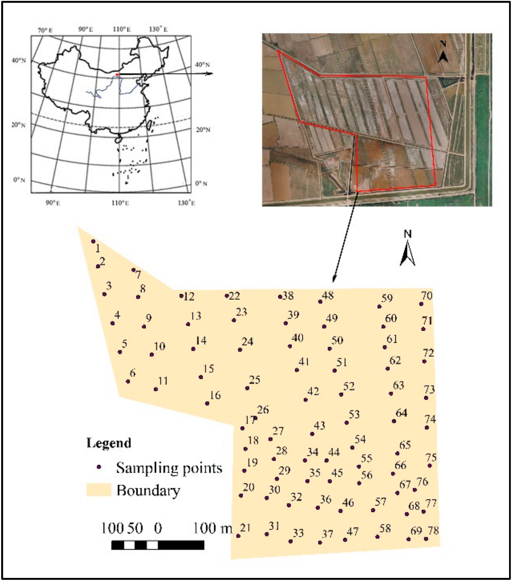
2.1. Site Description

The study area is located in the eastern part of the Hetao Irrigation District, northern China (Figure 1). It has a typical arid climate, with low precipitation and very high evapotranspiration. The annual precipitation is about 130–350 mm, and the annual temperature is about 5.6–7.4 °C [22]. The soil type is solonchak, according to World Reference Base for Soil Resources. The soil texture is clay loam with sand, silt, and clay contents of 24.11%, 43.60%, and 32.29%. The underground water table is high due to the frequent irrigation conducted every year. The average amount of irrigation water derived from the Yellow River every year is about 30–40 cm. The total dissolved salt in the Yellow River is about 0.5%. Thus, a great deal of salt has been added to the irrigated fields every year through irrigation. However, the drainage system is low compared to the irrigation system, i.e., only 10%. Thus, high irrigation and low drainage is a serious problem in the study area. The study area is next to Ulansuhai Lake, a drainage lake in the Hetao Irrigation District. Therefore, the water table in the study area is low and only varies by 0.5–1.5 m throughout the year. This has resulted in significant salinization in the area.

2.2. Soil Sampling and Laboratory Measurements

From the study field site (size in ha), soil bag samples from the topsoil (0–20 cm) and the subsoil (20–40 cm) at 78 sampling points were taken (Figure 1), which adds up to 156 soil bag samples. Then, they were taken to the laboratory and were air-dried and ground in preparation for analysis. The soil properties, including the pH, Na⁺, Ca²⁺, Mg²⁺, total salt content (TSC), SOM, sand content, silt content, and clay content, were measured. The pH was measured using a pH meter (Sartorius PB10). The Na⁺ content was measured using a flame photometer, and the Ca²⁺ and Mg²⁺ contents were measured via ethylene diamine tetraacetic complexometric acid titration [28]. The SOM was measured using the oxidation of the potassium dichromate external heating method [29]. The SAR was calculated using the Na⁺, Ca²⁺, and Mg²⁺ contents and the following formula, in which the unit of the ion concentrations is mmol L⁻¹ [13]. Soils with SARs of greater than 12, exchangeable sodium percentages (ESPs) of greater than 15, and EC values of greater than 5 pose a very high hazard to plant growth [7].

$$\mathrm{SAR}=\frac{{\mathrm{Na}}^{+}}{\sqrt{\frac{{\mathrm{Ca}}^{2+}+{\mathrm{Mg}}^{2+}}{2}}}$$

(1)

2.3. Geostatistical Analysis and Interpolation Methods

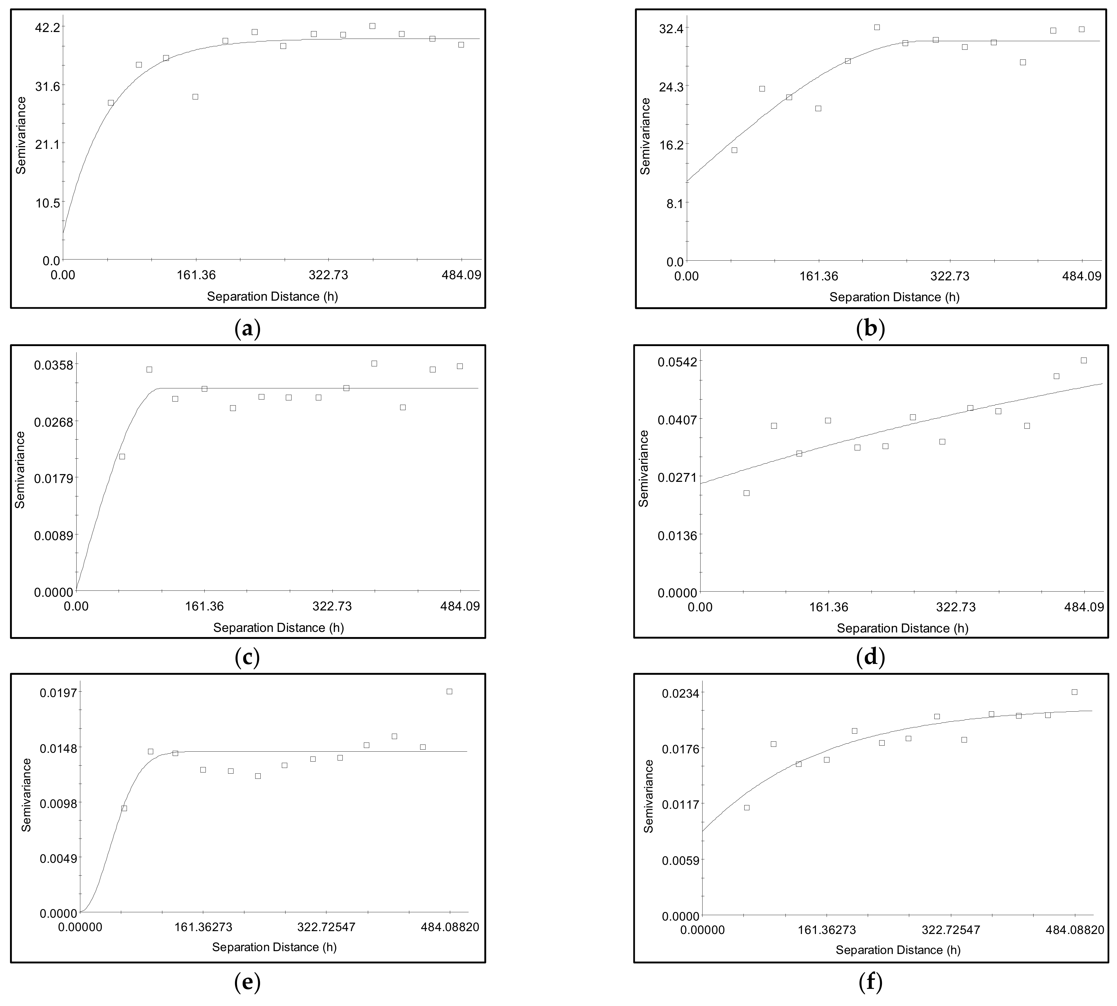
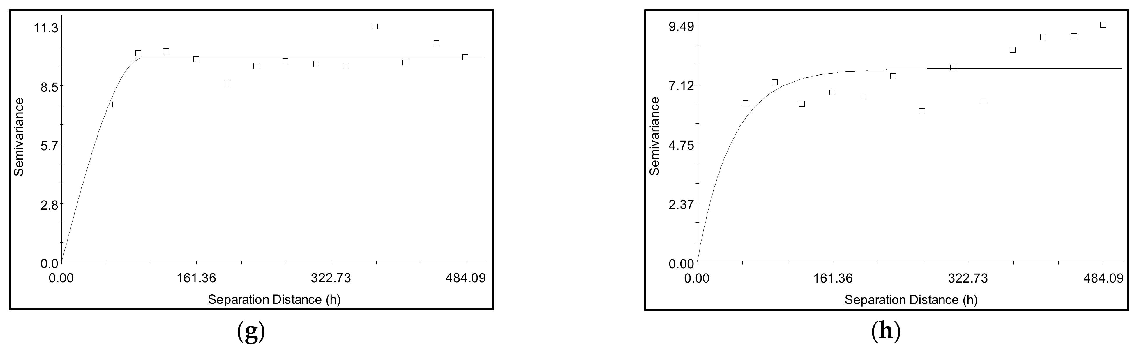
2.3.1. Semivariance Modeling

Semivariance modeling is widely used in geostatistical analysis. In soil science, the soil properties are always considered to be regionalized variables. The semivariance (γ(h)) of a considered soil property can be calculated as follows [30]:

$$\mathsf{\gamma }\left(\mathrm{h}\right)=\frac{1}{2\mathrm{N}\left(\mathrm{h}\right)}{{\displaystyle \sum }}_{\mathrm{i}=1}^{\mathrm{N}\left(\mathrm{h}\right)}{\left[\mathrm{Z}\left({\mathrm{x}}_{\mathrm{i}}\right)-\mathrm{Z}\left({\mathrm{x}}_{\mathrm{i}}+\mathrm{h}\right)\right]}^2,$$

(2)

where N(h) is the pair of points with lag distance h; Z(i) is the value of the considered property at point x_i, and Z(x_i + h) is the value of the property at a point a distance h away from point x_i.

Soil is a continuous spatial variable, and the semivariogram of a soil property is a continuous function. However, the semivariance is always calculated from a series of soil samples that contain discontinuities. Thus, the semivariance of these points can be simulated using curves, and the equation used for the curve fitting is called the theoretical model of the semivariogram. The commonly used models are the spherical model, the exponential model, and the Gaussian model:

$$\mathsf{\gamma }\left(\mathrm{h}\right)=\left\{\begin{array}{c}{\mathrm{C}}_0+\mathrm{C}\left(\frac{3\mathrm{h}}{2\mathrm{a}}-\frac{{\mathrm{h}}^3}{{\mathrm{a}}^3}\right)\hspace{1em}\hspace{1em}\hspace{1em}0\le \mathrm{h}\le \mathrm{a}\\ {\mathrm{C}}_0+\mathrm{C}\hspace{1em}\hspace{1em}\hspace{1em}\hspace{1em}\hspace{1em}\hspace{1em}\mathrm{h}\ge \mathrm{a}\end{array}\right.$$

(3)

$$\mathsf{\gamma }\left(\mathrm{h}\right)={\mathrm{C}}_0+\mathrm{C}\left(1-{\mathrm{e}}^{-\frac{\mathrm{h}}{\mathrm{a}}}\right)$$

(4)

$$\mathsf{\gamma }\left(\mathrm{h}\right)={\mathrm{C}}_0+\mathrm{C}\left(1-{\mathrm{e}}^{-\frac{{\mathrm{h}}^2}{{\mathrm{a}}^2}}\right)$$

(5)

where γ(h) is the semivariance; h is the lag distance; C₀ is the nugget, and C is the sill. C₀/(C₀ + C) can reflect the degree of spatial dependence. The spatial dependence is divided into strong (C₀/(C₀ + C) < 25%), moderate (25% ≤ C₀/(C₀ + C ≤ 75%), and weak (C₀/(C₀ + C) > 75%) dependence [31]. The simulation is done in professional geostatistical software (GS + 9.0). The software simulated the data with all three models and compared the R² of them. The best model is chosen with the highest R² value.

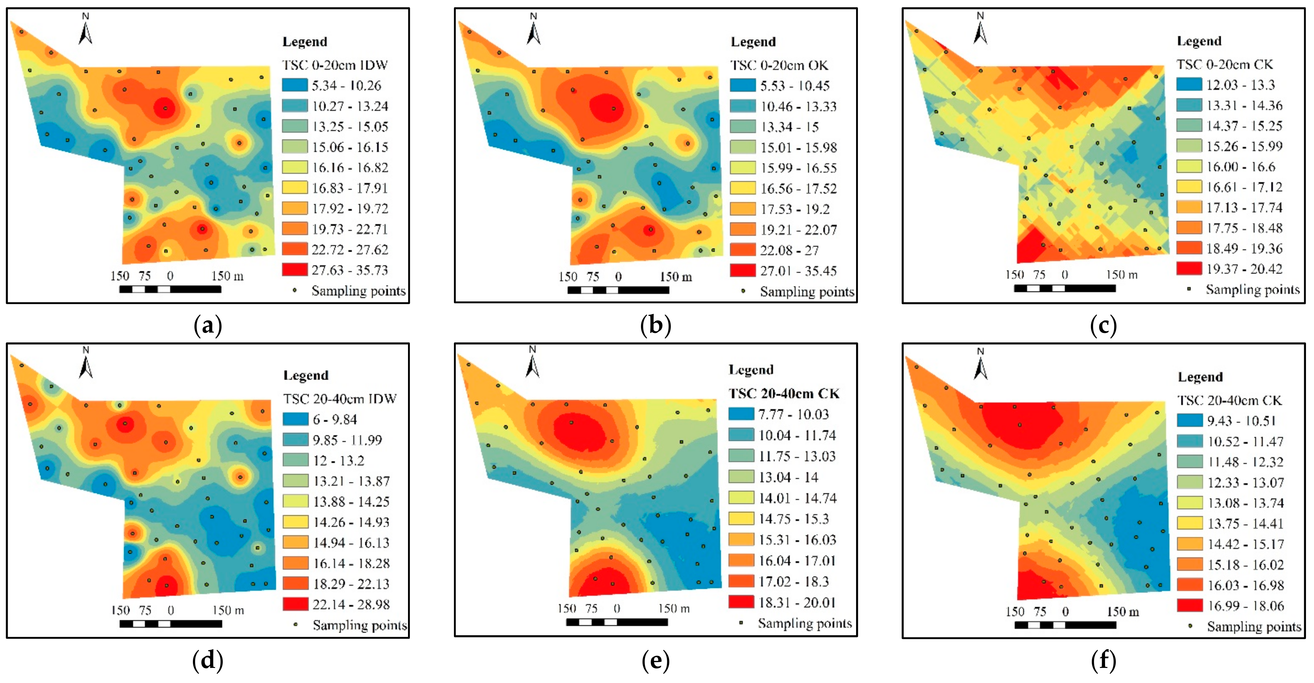
2.3.2. Inverse Distance Weighting Interpolation

The IDW method is a widely used, straightforward, noncomputational interpolation method. The predicted value (P_j) for location j is calculated based on the distance weight [15].

$${\mathrm{P}}_{\mathrm{j}}={{\displaystyle \sum }}_{\mathrm{i}=1}^{\mathrm{n}}{\mathsf{\lambda }}_{\mathrm{i}}{\mathrm{O}}_{\mathrm{i}}.$$

(6)

where O_i is the observed value at location i; and λ_i is the weight, which can be calculated as

$${\mathsf{\lambda }}_{\mathsf{i}}={\mathsf{d}}_{\mathsf{ij}}^{-\mathsf{\alpha }}/{\displaystyle \sum }_{\mathsf{i}=1}^{\mathsf{n}}{\mathsf{d}}_{\mathsf{ij}}^{-\mathsf{\alpha }}$$

(7)

In this equation, d_ij is the distance between i and j; and α is a specified value, which is always larger than 1 and is always taken to be 2 [32]. As can be seen, points closer to the target location have greater weights.

2.3.3. Ordinary Kriging Interpolation

Ordinary kriging is a widely used interpolation method, which can be used to obtain an optimal, linear, and unbiased prediction for a nonsampled point based on the values of neighboring sample points. The OK method assigns weights to these points based on their distances from the point being estimated and the spatial variability structure, and the formula is as follows [21,33]:

$$\mathrm{Z}\left({\mathrm{x}}_0\right)={{\displaystyle \sum }}_{\mathrm{i}=1}^{\mathrm{n}}{\mathrm{w}}_{\mathrm{i}}\mathrm{Z}\left({\mathrm{x}}_{\mathrm{i}}\right).$$

(8)

In this equation, Z(x₀) is the predicted value; and w_i is the weight for ith observation value Z(i). To obtain an optimal and unbiased prediction, the sum of the weights must be equal to 1, and the estimation or kriging variance is minimized.

2.3.4. Cokriging Interpolation

In the IDW and OK predictions, the only parameter used to determine the weight is the distance. Variables that have spatial relationships with two or more variables can be predicted using the cokriging method:

$${\mathrm{Z}}_{\mathrm{u}}\left(\mathrm{b}\right)={{\displaystyle \sum }}_{\mathrm{I}}^{\mathrm{V}}{{\displaystyle \sum }}_{\mathrm{i}=1}^{\mathrm{n}}{\mathrm{w}}_{\mathrm{iI}}{\mathrm{Z}}_{\mathrm{I}}\left({\mathrm{x}}_{\mathrm{i}}\right)$$

(9)

In this equation, Z_u(b) is the predicted variable u; and V is the number of related variables. N is the number of pairs of points. w_iI is the weight of the Ith variable at point i, and Z_I(x_i) is the observed matrix value for the Ith variable at point i. To obtain an optimal and unbiased prediction, the sum of the weights of the predicted properties must be 1, and that of the other properties must be 0 [33]:

$${{\displaystyle \sum }}_{\mathrm{i}=1}^{\mathrm{n}}{\mathrm{w}}_{\mathrm{i}}\mathrm{Z}\left({\mathrm{x}}_{\mathrm{i}}\right)=\left\{\begin{array}{c}1 \mathrm{I}=\mathrm{u}\\ 0 \mathrm{I}\ne \mathrm{u}\end{array}\right.$$

(10)

In addition, the estimation or the cokriging variance should be minimized. In this study, soil texture (sand content, silt content, or clay content) was selected as the covariance in the cokriging prediction. This is mainly because the soil texture forms the basis of the soil structure and strongly affects the leaching of salt [14].

2.4. Validation of the Different Interpolation Methods

A total of 78 points were sampled in the study area. Thirty of them were selected as validation data, and the other 48 points were used as interpolation data. The IDW, ordinary kriging, and cokriging methods were used to predict the TSC, pH, LogSAR, and SOM values for both the surface and subsurface layers in ArcMap 10.6. Then, the prediction maps were converted to raster style, and the predicted values of the validation points were extracted using the “Extract value to points” tool in ArcMap. Thereafter, the Root Mean Squared Error (RMSE) of the predicted value for each soil property was calculated as

$$\mathrm{RMSE}=\sqrt{\frac{1}{\mathrm{m}}{{\displaystyle \sum }}_{\mathrm{i}=1}^{\mathrm{m}}{\left({\mathrm{y}}_{\mathrm{i}}-{\mathrm{y}}_{\mathrm{j}}\right)}^2}$$

(11)

where m is the total number of validation points, y_i is the observed value, and y_j is the predicted value. For a given property, the lower the RMSE, the more accurate the method. The regression analysis of the predicted and observed values were also conducted in SPSS 22.0. A higher coefficient of determination (R²) means more variance was interpreted using the predicted method.

3. Results

3.1. Statistical Analysis and Data Distribution of the Studied Soil Properties

The mean TSC values are 16.4 g/kg and 13.42 g/kg for the surface and subsurface soil layers, respectively (

Table 1. Statistical analysis of the soil salinity and other properties for the different layers.

Index	Layer	Min	Max	Mean	SD	CV
TSC	0–20 cm	5.33	35.75	16.40 a	6.22	0.38
(g/kg)	20–40 cm	5.52	28.54	13.42 b	5.10	0.38
pH	0–20 cm	8.23	8.89	8.51 a	0.17	0.02
	20–40 cm	8.01	9.00	8.57 a	0.21	0.03
SAR	0–20 cm	24.44	100.79	55.64 a	16.63	0.30
	20–40 cm	25.86	100.17	49.79 b	16.76	0.34
SOM	0–20 cm	6.08	23.50	14.19 a	3.38	0.24
(g/kg)	20–40 cm	7.46	21.89	13.08 b	2.92	0.22
Sand	0–20 cm	6.45	39.49	22.99 a	7.90	0.34
(%)	20–40 cm	10.12	41.34	25.27 a	7.84	0.31
Silt	0–20 cm	34.53	60.30	45.58 a	5.73	0.13
(%)	20–40 cm	32.63	54.24	41.02 b	5.34	0.13
Clay	0–20 cm	7.36	50.68	31.43 a	10.54	0.34
(%)	20–40 cm	5.27	48.02	33.70 b	10.46	0.31

CV–coefficients of variation, SD–standard deviation, SAR–sodium adsorption ratio, TSC–total salt concentration, SOM–soil organic matter. The letter after the mean value means the difference is significant at 0.05 level.

). The TSC of the surface soil layer is significantly higher than that of the subsurface soil layer. However, the coefficients of variation (CVs) for the soil layers are similar. The TSC is significantly higher in the surface layer than in the subsurface layer. The SAR and SOM are also significantly higher in the surface layer than in the subsurface layer. The CVs are also similar for the two layers, both of which indicate moderate variation. Unlike these properties, pH has both similar mean values and CVs for the two soil layers. Moreover, the CVs indicate weak variation. The surface layer’s sand, silt, and clay contents were 22.99%, 45.58%, and 31.43%. However, they were 25.27%, 41.02%, and 33.70% for the subsurface layer. Although the sand, silt, and clay contents all exhibit moderate variation, the variations in the silt contents of both layers are close to being weak. The data for the soil properties exhibit normal distributions, except for SAR for both layers and the sand content of the subsurface layer, which obey normal distributions after log transformation (

Table 2. Kolmogorov-Smirnov test for the data distribution.

Soil Layer	TSC	pH	LogSAR	SOM	Sand	Silt	Clay
0–20 cm	0.196	0.533	0.2 *	0.2	0.2	0.2	0.2
20–40 cm	0.067	0.2	0.2 *	0.2	0.08 *	0.2	0.06

* means the data were transformed using a logarithmic transformation.

).

3.2. Geostatistical Analysis of the Soil Salinity and Related Soil Properties

The considered soil properties exhibit a clear nugget effect, except for the pH of the surface layer, SAR of the surface layer, and the SOM in both layers (Figure 2). The exponential model best fits the TSC for the surface layer and the subsurface layer’s spherical model. The nugget/sill values for the surface and subsurface soil layers are 11.76% and 36.12%, respectively (

Table 3. Geostatistical analysis of the considered soil properties.

Index	Soil Layer	Model	C0	C0 + C	C0/(C0 + C) (%)	Range (m)	R2
TSC	0–20 cm	Exponential	4.7000	39.95	11.76	170.4	0.62
	20–40 cm	Spherical	11.0000	30.45	36.12	291.7	0.81
pH	0–20 cm	Spherical	0.0001	0.0319	0.31	107.3	0.56
	20–40 cm	Exponential	0.0253	0.0792	31.94	2645.1	0.62
LogSAR	0–20 cm	Gaussian	0.0000	0.0143	0.14	95.3	0.34
	20–40 cm	Exponential	0.0087	0.0220	43.95	469.8	0.77
SOM	0–20 cm	Spherical	0.0100	9.81	0.10	98.3	0.48
	20–40 cm	Exponential	0.0100	7.73	0.13	127.2	0.14

LogSAR means the SAR has been transferred to a normal distribution using a log transformation, C₀–nugget value, and C–sill value.

). This suggests a strong spatial dependence for the surface layer but a moderate spatial dependence for the subsurface layer. The range for the surface layer (170.4 m) is much smaller than that for the subsurface layer (291.7 m). R² of the subsurface layer (0.81) is higher than the surface layer (0.62). For the other soil properties, the values for the surface layer are best fitted by the spherical model and those of the subsurface layer by the exponential model.

Moreover, the nugget/sill values for the pH and SAR for the surface layer are much higher (moderate spatial dependence) than those for the subsurface layer (strong spatial dependence). However, for the SOM, both layers exhibit a strong spatial dependence. The ranges of the pH, SAR, and SOM values for the surface layer are much higher than those for the subsurface layer, indicating a longer spatial correlation for the subsurface layer.

3.3. Correlations between Soil Salinity and Other Soil Properties

In the surface layer, the TSC was significantly negatively correlated with the pH and the clay content, but it was very significantly positively correlated with the silt content at the p < 0.01 level (

Table 4. The correlation matrix of the considered soil properties.

Soil Layer	Index	Parameter	TSC	pH	SOM	Log SAR	Sand	Silt	Clay
0–20 cm	TSC	R	1	−0.297 **	0.14	0.314 **	0.175	0.397 **	−0.362 **
		p		0.008	0.221	0.005	0.125	0	0.001
	pH	R		1	0.105	0.517 **	−0.205	−0.337 **	0.350 **
		p			0.362	0	0.072	0.003	0.002
	SOM	R			1	0.029	−0.311 **	0.08	0.195
		p				0.798	0.006	0.484	0.087
	Log SAR	R				1	−0.164	−0.085	0.175
		p					0.152	0.461	0.125
	Sand	R					1	0.088	−0.824 **
		p						0.445	0
	Silt	R						1	−0.637 **
		p							0
	Clay	R							1
		p
20–40 cm	TSC	R	1	−0.521 **	0.041	0.466 **	0.173	0.405 **	−0.378 **
		p		0	0.724	0	0.13	0	0.008
	pH	R		1	0.288 *	0.153	−0.317 **	−0.275 *	0.452 **
		p			0.011	0.181	0.005	0.015	0.001
	SOM	R			1	0.200	−0.365 **	−0.007	0.305 **
		p				0.079	0.001	0.951	0.035
	Log SAR	R				1	−0.177	0.036	0.133
		p					0.120	0.752	0.244
	Sand	R					1	−0.078	−0.882 **
		p						0.5	0
	Silt	R						1	−0.615 **
		p							0
	Clay	R							1
		p

* means the correlation is significant at the 0.5 level, and ** means the correlation is significant at the 0.01 level.

). The TSC was significantly correlated with LogSAR at the p < 0.05 level. No significant correlations were found between the TSC and the SOM and sand content. The subsurface layer exhibits very similar correlations between the TSC and other soil properties. However, the correlation coefficients were higher than those for the surface layer, especially for the pH and LogSAR. The other soil properties exhibited significant pair correlations, especially with soil texture. The silt and clay contents were significantly correlated with the TSC and pH in both the surface and subsurface layers. The SOM was significantly correlated with the sand content in the surface layer and correlated with the sand content and clay content in the subsurface layer. Although the soil texture was not significantly correlated with LogSAR, the correlation between the clay content and LogSAR for the surface layer was significant at the p < 0.1 level. Therefore, the soil texture, which exhibits significant correlations with the considered soil properties, was input as a covariable in the CoKriging prediction.

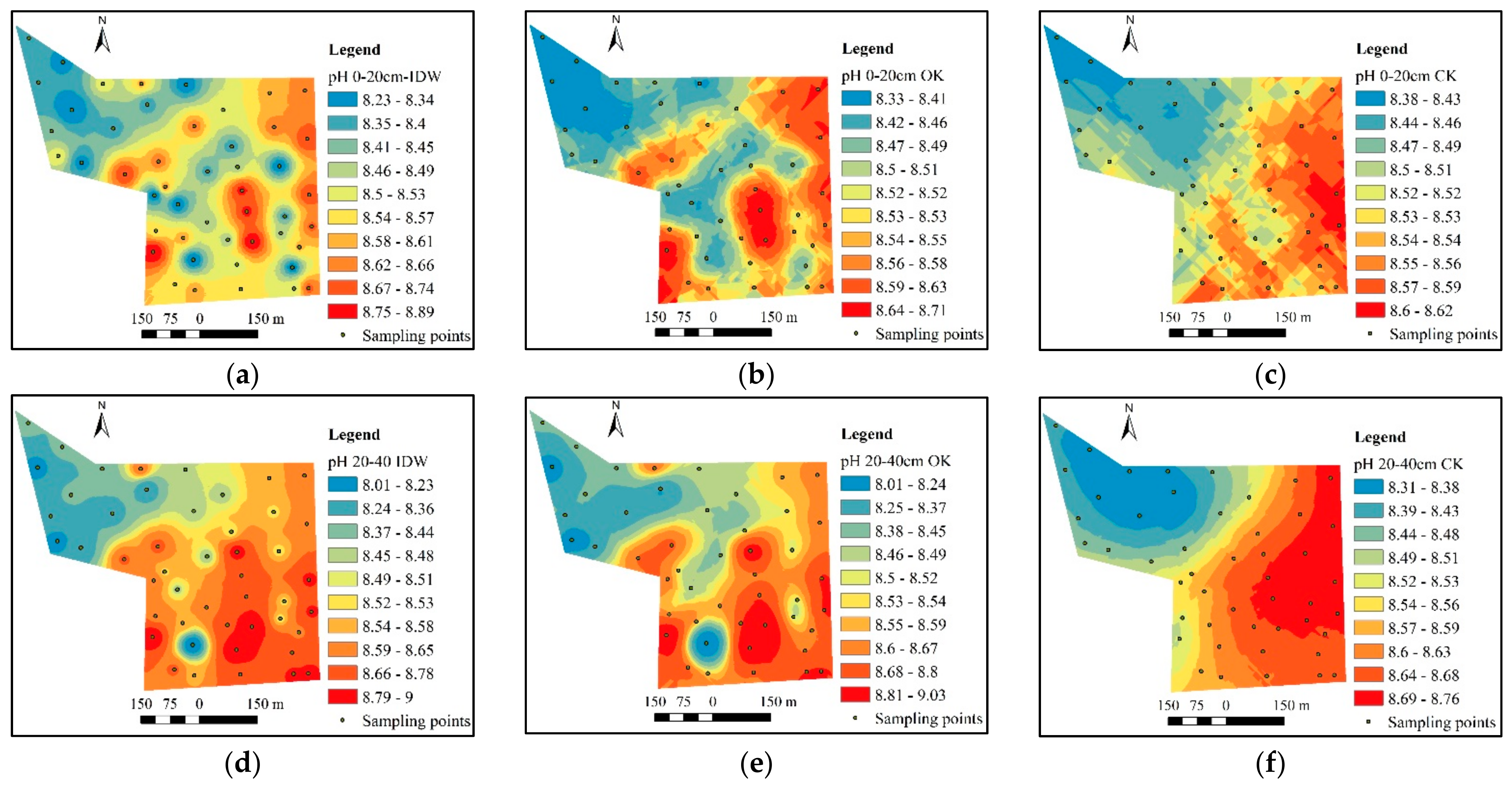
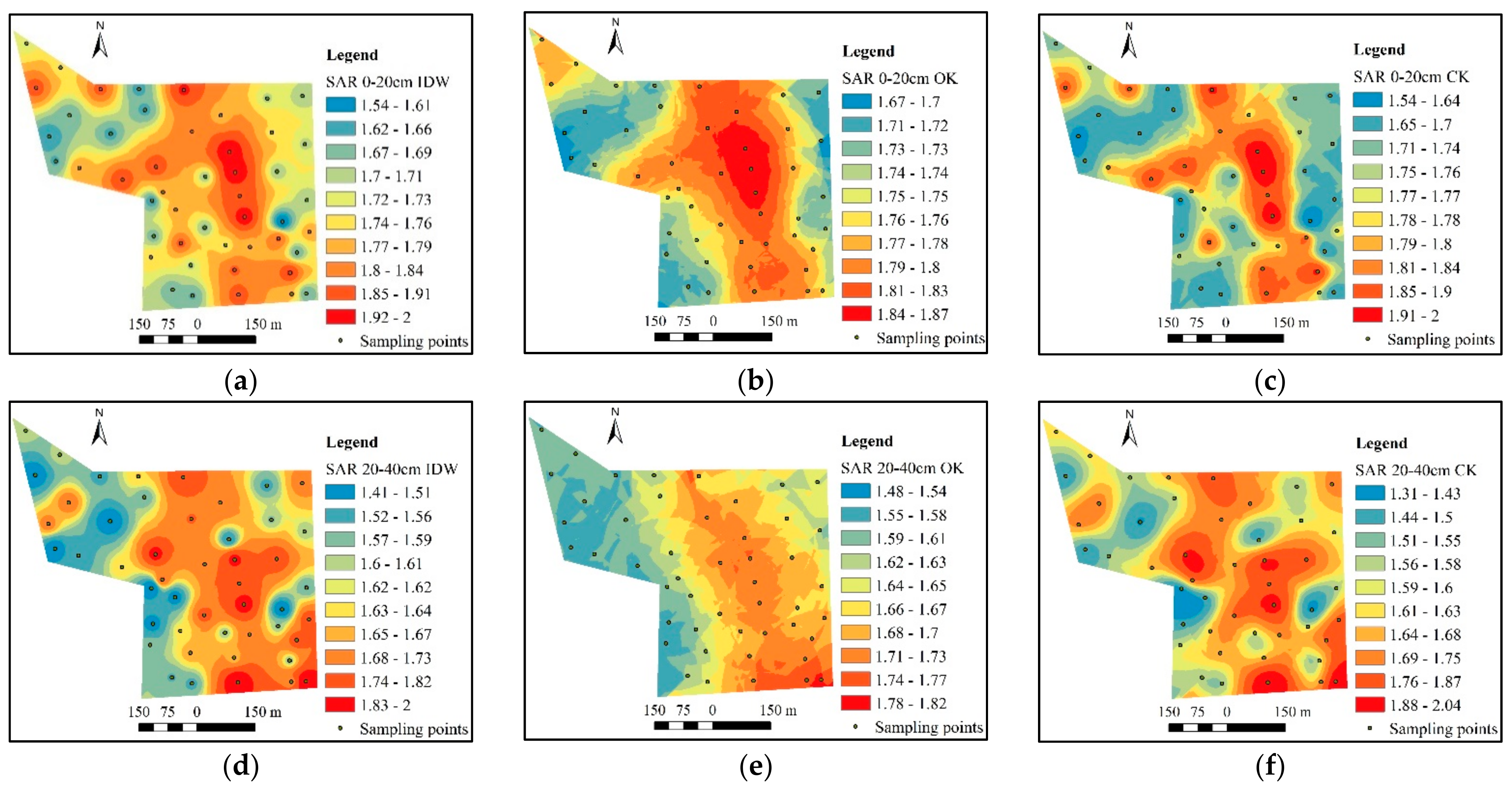
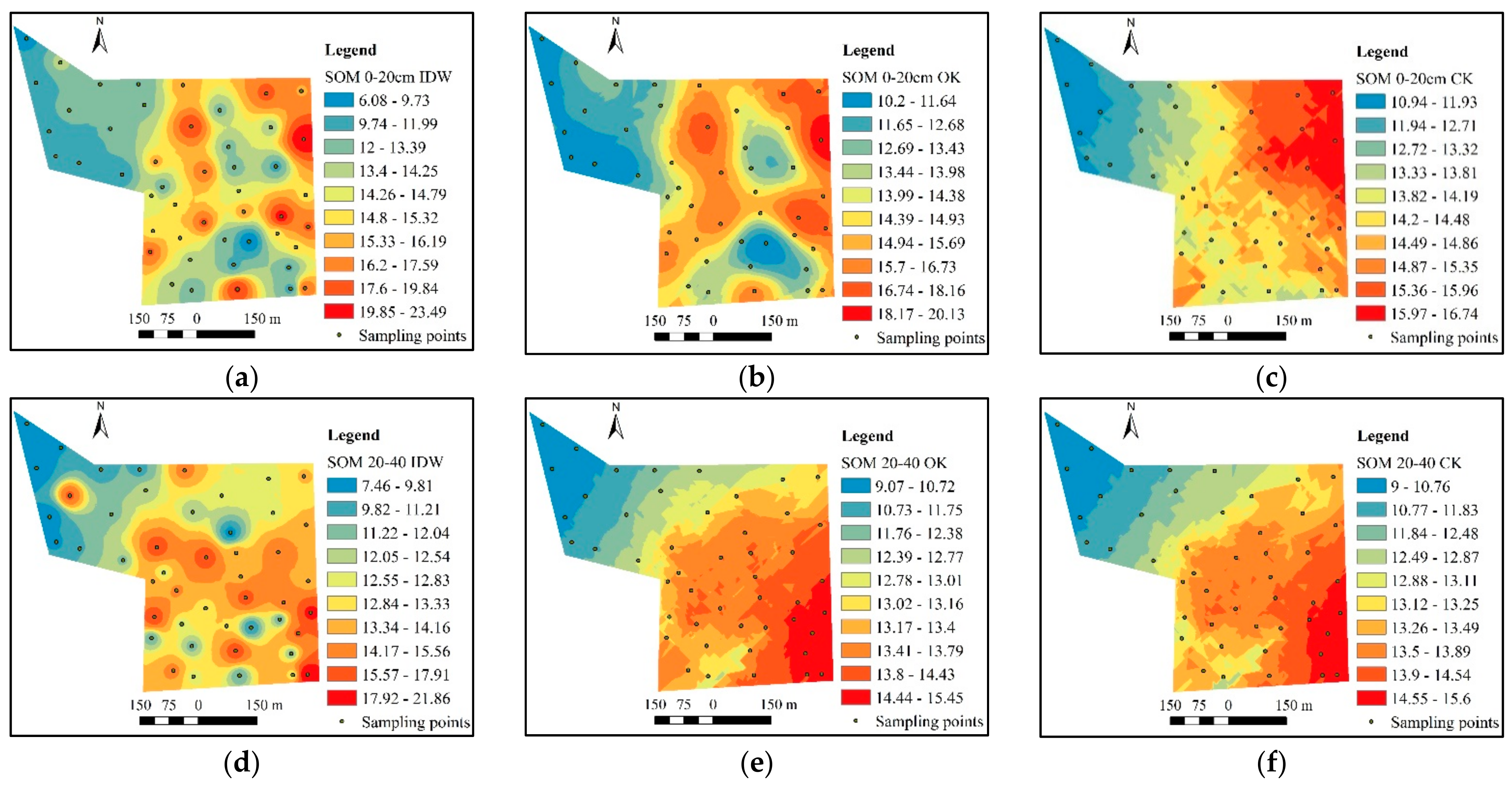
3.4. Spatial Distributions of the Soil Salinity and Other Soil Properties Predicted Using the Different Methods

The general trends of the spatial distributions of the soil properties obtained using the different methods were similar. However, the IDW method showed a clearer patch than the other methods (Figure 3, Figure 4, Figure 5 and Figure 6). The cokriging method was the most homogeneous compared to the other two interpolation methods. For the TSC of the surface layer, all methods produced higher value zones in the north and south and a lower value zone in the middle of the study area (Figure 3). The higher and lower value zones are clearer for the subsurface layer than for the surface layer. The higher value zone is mainly located in the central-north and southwest areas, but the lower value zone is located in the southeastern part of the study area. The pH values exhibited a different spatial distribution than the TSC, mainly decreasing from southeast to northwest (Figure 4).

Moreover, the two soil layers exhibit similar spatial distributions. The spatial distribution of the SAR firstly increases and then decreases from west to east. The highest value zones appear in the middle part for the surface layer and in the southeast part for the subsurface layer (Figure 5). The SOM showed a similar trend with the pH value. However, SOM exhibits different spatial distributions in the two layers (Figure 6). The higher value zone is mainly located in the northeast for the surface layer, but in the subsurface layer, the higher value zone is mainly located in the southwest.

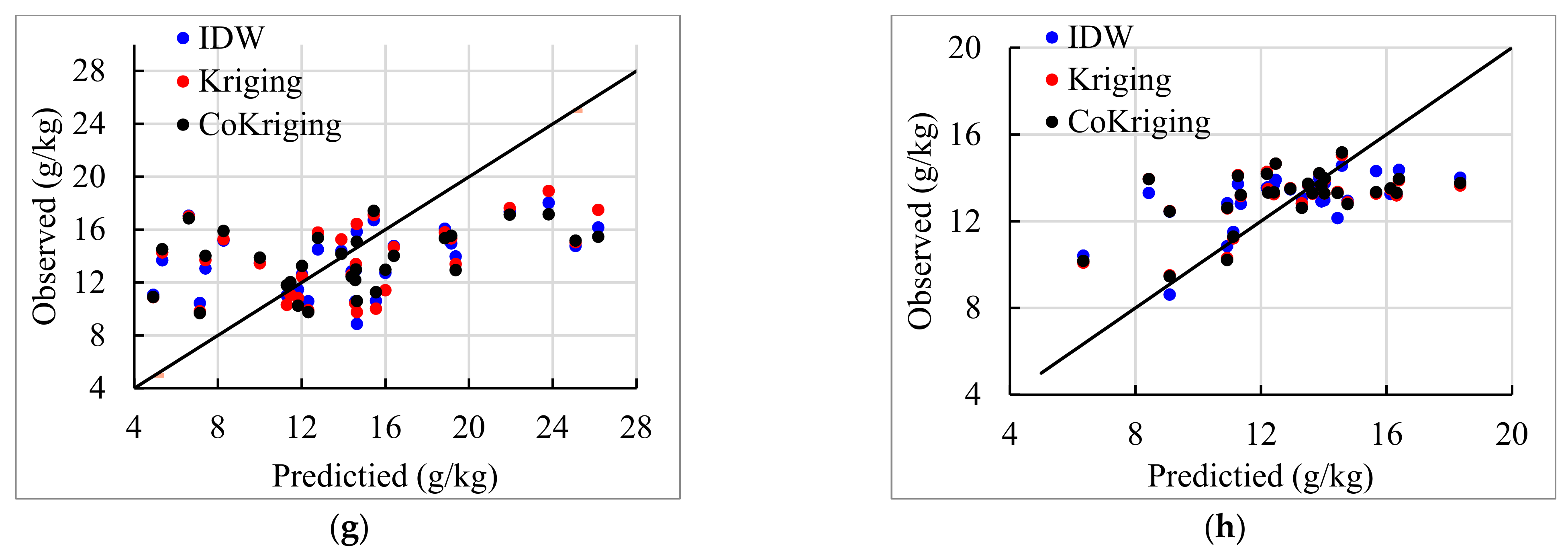
3.5. Comparison of the Different Prediction Methods

For the TSC of the surface layer, the cokriging method performed the best, but the kriging method performed the best (

Table 5. RMSEs of the different methods used to predict the soil properties.

Index	Soil Layers	IDW	OK	CK	Best Method
TSC	0–20 cm	4.78	5.08	4.68	CoKriging
	20–40 cm	4.96	4.95	5.10	Kriging
pH	0–20 cm	0.16	0.17	0.18	IDW
	20–40 cm	0.18	0.17	0.19	Kriging
Log SAR	0–20 cm	0.13	0.15	0.14	IDW
	20–40 cm	0.11	0.10	0.13	Kriging
SOM	0–20 cm	2.63	2.74	2.72	IDW
	20–40 cm	2.58	2.65	2.62	IDW

). For the pH and SAR of the surface layer and the SOM in both layers, the IDW method performed the best. For the pH and SAR of the subsurface layer, the kriging and cokriging performed the best, respectively. The scatter plot shows that the TSC for both layers, the pH for the subsurface layer, and the SOM for the surface layer exhibited a more decentralized trend (Figure 7), indicating the larger uncertainty of the prediction.

4. Discussion

4.1. Soils Salinity of the Different Soil Layers and Its Correlation with the Other Properties

The soil salinity is usually higher for the surface soil layer than for the subsurface layer, especially for secondary salinization (or man-made soil salinization). Our study area’s TSC of the surface layer is 16.40 g/kg, significantly higher than that of the subsurface layer (13.42 g/kg) (Table 1). The same phenomenon was observed in a study in a reclaimed area of the Behera Governorate of Egypt. The concentrations of the main ions were higher in the surface layer than in the subsurface layer [20]. Still, the studied soil depths were different than those used in our study. In the Igdir Plain (Turkey), researchers have also found a decrease in EC with depth in the soil profile [3]. Another study found that the EC was higher in the surface layer than in the deeper layers, and the deeper layers did not exhibit significant differences [34]. In Xinjiang Province, northern China, the EC values in the surface soil layer (0–10 cm) were found to be significantly higher than at the 10–20 cm and 20–30 cm soil layers [35]. The general trend indicated salt aggregation in the surface soil. This was mainly caused by shallow underground saline water, which moved up through the soil due to capillary action and evaporation [10]. When the saline water reached the soil surface, the water evaporated into the air, and the salt was left behind in the soil. The soil salinity exhibited a moderate variation in our study. The soil EC was also found to exhibit a moderate variation (CV of EC was 47.4%) in the southeastern part of Algeria [21] and in the Manas River watershed in northern China (CV of EC was 33.1–63.0%) [10], but their CV values were higher than those in our study (Table 1). Another study reported a strong variation (CVs of 1.31–1.57) in the different soil layers [35]. The CVs of the different EC datasets may also differ. For example, in the coastal agricultural areas of northern Iran, the CV of the 0–50 cm layer was 56.7%, indicating moderate variation, but it was 114.7% for the 50–100 cm layer (strong variation). In our study, the variation in the two layers was the same. This may be caused by the higher sampling thickness (20 cm). Therefore, a thinner sample should be conducted in future studies.

Soil salinity can exhibit a positive [21] or negative [36] correlation with pH, but the correlation is generally not significant. In our study, a significant negative correlation was found between TSC and pH in both soil layers. This was mainly caused by the fact that the main cation in the soil in our study area is sodium. When the TSC decreases, the sodium ion concentration mainly decreased. This caused the proportion of divalent cations (Ca²⁺ and Mg²⁺) to increase. In addition, the proportion of bicarbonate in the anions increased, while that of sulfate decreased. This caused an increase in the soil pH [37]. The soil salinity is positively correlated with the SAR in our study area (Table 3), and similar results have been found in other studies [6,7,10]. This indicated that soil salinity might increase soil alkalinity. A previous study found that saline soils are characterized by relatively high SAR values (7.31–52.10), which are significantly higher than those of non-saline soils (2.66–9.53) [5]. The SAR values in our study were much higher than the values in their study, indicating more severe soil alkalinity. The soil texture had a significant influence on the soil salinity, and it may predominantly control the soil salinity distribution. The silt content had a significant positive correlation with soil salinity, but the sand content had a significant negative correlation with soil salinity [38]. Another study reported a significant positive correlation between soil salt content and sand content, but it was negatively correlated with the clay content [14]. We found that the TSC is significantly positively correlated with the silt content, but it is significantly negatively correlated with the clay content (Table 4). This may be because the capillary force is higher in silt, which may increase the accumulation of salt on the surface. However, the capillary force is lower in clay soils, so salt accumulation on the surface may be low.

4.2. Geostatistical Characteristic of Soil Salinity in the Arid Irrigation Region in Northern China

The semivariance of the salinity of the surface soil is fitted best by the exponential model, but the subsurface soil is fitted best by the spherical model (Table 3). A previous study reported different results and showed that the spherical model was best for the surface soil layer and the exponential model was best for the subsurface soil layer [3]. Studies have also reported that all of the soil profile layers are fitted best by the spherical model [4,18]. These different results may be caused by different sampling times and sampling strategies. The nugget effect increases with soil depth, although both of the layers in our study exhibit a moderate spatial dependence. One study reported that the surface layer has a strong spatial dependence, but the bottom layer has a moderate spatial dependence [18]. Other results indicate that, in general, the nugget/sill value decreases with soil depth [39]. The spatial dependence of soil salinity is different in different regions and at different times, affecting the spatial distribution predicted using the kriging method. Except for the TSC, all of the other soil properties showed a lower nugget effect for the surface soil layer than for the subsurface soil layer. In addition, the nugget/silt value was much lower for the surface layer. This indicates that the spatial dependence of the soil properties was higher in the surface soil layer.

4.3. The Best Method for Predicting Soil Salinity in the Arid Irrigation Distinct

Many researchers have evaluated the performances of the different interpolation methods. The results almost always differ. In a newly reclaimed area in the southern part of the Behera Governorate of Egypt, the IDW method outperformed the other methods, including the ordinary kriging, regression kriging, and cokriging methods [20]. In the agricultural coastal areas of northern Iran, the OK method had the minimum error compared with the IDW and conditional simulations methods [18]. In the southern part of the Arkansas River Basin in Colorado, USA, the performances of the different geostatistical models were as follows: ordinary kriging > regression kriging > cokriging [40]. In other words, the applicability of the spatial prediction methods to a specific soil in a specific region are still unknown. In our study area, different methods were found to be optimal for the different soil properties and soil layers (Table 5). We found that the optimal methods are closely related to the relationship between the nugget/sill value and the range of the considered soil properties values (Figure 8). The soil properties with lower nugget/sill values and smaller ranges are best predicted using the IDW method. The soil properties with intermediate nugget/sill values and value ranges are best predicted using the CK method. The soil properties with higher nugget/sill values and larger ranges are best predicted using the OK method. This may be caused by the different calculation methods used by the different prediction methods. The kriging method is a function of the statistical stationarity, while the IDW is a function of the distance between the sampling points [32]. When both the nugget/sill value and the range are lower, the property has a strong spatial dependence in a short distance. This condition may be more in accord with the assumptions of the IDW method.

5. Conclusions

The average TSCs were 16.40 g/kg and 13.42 g/kg for the surface (0–20 cm) and subsurface (20–40 cm) soil layers in a typical piece of salt-affected land in the arid irrigation region, northern China. In addition, the SAR was also extremely high, i.e., 55.64 for the surface soil and 49.79 for the subsurface soil layers. This suggests that both soil salinization and alkalization are serious problems in this area. Compared to the other soil properties, the TSC and SAR have higher CV values, indicating a higher variance in the soil salinity and alkalinity. The nugget/sill values of the TSC are 11.76% and 36.12% for the surface and subsurface soil layers, respectively. This indicates that the soil salinity has a moderate spatial dependence. The TSC is significantly correlated with the soil texture (mainly the silt and clay contents), but the LogSAR is not correlated with the soil texture. This indicates that the soil texture may more easily influence the soil salinity. The general trends of the prediction maps of the considered soil properties obtained using the three different methods (IDW, OK, and CK) are similar. However, the OK and CK methods produced more homogeneous results than the IDW method. The RMSEs of the different methods showed that the TSC was predicted best using the cokriging (surface) and kriging (subsurface) methods. The pH and SAR were predicted best using the IDW (surface) and kriging (subsurface) methods, and the SOM was predicted best using the IDW (both layers) method. This may be determined by both the nugget/sill values and value ranges of the predicted properties. Lower nugget/sill values and smaller ranges may be fitted best using the IDW method, while higher nugget/sill values and larger ranges may be fitted best using the OK method. These results provide a powerful basis for the spatial prediction of soil salinity and provide useful information for irrigation, fertilization, and other land management measures.

References

1. Shrivastava, P.; Kumar, R. Soil salinity: A serious environmental issue and plant growth promoting bacteria as one of the tools for its alleviation. Saudi J. Biol. Sci. 2015, 22, 123–131. [Google Scholar] [CrossRef] [PubMed] [Green Version]
2. Bartels, D.; Sunkar, R. Drought and Salt Tolerance in Plants. Crit. Rev. Plant Sci. 2005, 24, 23–58. [Google Scholar] [CrossRef]
3. Ardahanlioglu, O.; Oztas, T.; Evren, S.; Yilmaz, H.; Yildirim, Z.N. Spatial variability of exchangeable sodium, electrical conductivity, soil pH and boron content in salt- and sodium-affected areas of the Igdir plain (Turkey). J. Arid Environ. 2003, 54, 495–503. [Google Scholar] [CrossRef]
4. Juan, P.; Mateu, J.; Jordan, M.M.; Mataix-Solera, J.; Meléndez-Pastor, I.; Navarro-Pedre, O.J. Geostatistical methods to identify and map spatial variations of soil salinity. J. Geochem. Explor. 2011, 108, 62–72. [Google Scholar] [CrossRef]
5. Al-Busaidi, A.S.; Cookson, P. Salinity–pH Relationships in Calcareous Soils. J. Agric. Mar. Sci. JAMS 2003, 8, 41–46. [Google Scholar] [CrossRef] [Green Version]
6. Ivushkin, K.; Bartholomeus, H.; Bregt, A.K.; Pulatov, A.; Kempen, B.; de Sousa, L. Global mapping of soil salinity change. Remote Sens. Environ. 2019, 231, 111260. [Google Scholar] [CrossRef]
7. Shrestha, R.P. Relating soil electrical conductivity to remote sensing and other soil properties for assessing soil salinity in northeast Thailand. Land Degrad. Dev. 2006, 17, 677–689. [Google Scholar] [CrossRef]
8. Burger, F.; Čelková, A. Salinity and sodicity hazard in water flow processes in the soil. Plant Soil Environ. 2003, 49, 314–320. [Google Scholar] [CrossRef] [Green Version]
9. Morrissey, E.M.; Gillespie, J.L.; Morina, J.C.; Franklin, R.B. Salinity affects microbial activity and soil organic matter content in tidal wetlands. Glob. Chang. Biol. 2014, 20, 1351–1362. [Google Scholar] [CrossRef]
10. Wang, J.; Liu, Y.; Wang, S.; Liu, H.; Fu, G.; Xiong, Y. Spatial distribution of soil salinity and potential implications for soil management in the Manas River watershed, China. Soil Use Manag. 2020, 36, 93–103. [Google Scholar] [CrossRef]
11. Liu, G.; Li, J.; Zhang, X.; Wang, X.; Lv, Z.; Yang, J.; Shao, H.; Yu, S. GIS-mapping spatial distribution of soil salinity for Eco-restoring the Yellow River Delta in combination with Electromagnetic Induction. Ecol. Eng. 2016, 94, 306–314. [Google Scholar] [CrossRef]
12. Akramkhanov, A.; Martius, C.; Park, S.J.; Hendrickx, J.M.H. Environmental factors of spatial distribution of soil salinity on flat irrigated terrain. Geoderma 2011, 163, 55–62. [Google Scholar] [CrossRef]
13. Xiao, Z.; Li, Y.; Feng, H. Modeling Soil Cation Concentration and Sodium Adsorption Ratio Using Observed Diffuse Reflectance Spectra. Can. J. Soil Sci. 2016, 96, 372–385. [Google Scholar] [CrossRef]
14. Fei, Y.; She, D.; Fang, K. Identifying the Main Factors Contributing to the Spatial Variability of Soil Saline–Sodic Properties in a Reclaimed Coastal Area. Vadose Zone J. 2018, 17, 180118. [Google Scholar] [CrossRef] [Green Version]
15. Lu, G.Y.; Wong, D.W. An adaptive inverse-distance weighting spatial interpolation technique. Comput. Geosci. 2008, 34, 1044–1055. [Google Scholar] [CrossRef]
16. Yamamoto, J.K. An Alternative Measure of the Reliability of Ordinary Kriging Estimates. Math. Geol. 2000, 32, 489–509. [Google Scholar] [CrossRef]
17. Vauclin, M.; Vieira, S.R.; Vachaud, G.; Nielsen, D.R. The Use of Cokriging with Limited Field Soil Observations. Soil Sci. Soc. Am. J. 1983, 47, 175–184. [Google Scholar] [CrossRef]
18. Emadi, M.; Baghernejad, M. Comparison of spatial interpolation techniques for mapping soil pH and salinity in agricultural coastal areas, northern Iran. Arch. Agron. Soil Sci. 2014, 60, 1315–1327. [Google Scholar] [CrossRef]
19. Robinson, T.P.; Metternicht, G. Testing the performance of spatial interpolation techniques for mapping soil properties. Comput. Electron. Agric. 2006, 50, 97–108. [Google Scholar] [CrossRef]
20. AbdelRahman, M.A.E.; Zakarya, Y.M.; Metwaly, M.M.; Koubouris, G. Deciphering Soil Spatial Variability through Geostatistics and Interpolation Techniques. Sustainability 2021, 13, 194. [Google Scholar] [CrossRef]
21. Abdennour, M.A.; Douaoui, A.; Piccini, C.; Pulido, M.; Bennacer, A.; Bradaï, A.; Barrena, J.; Yahiaoui, I. Predictive mapping of soil electrical conductivity as a Proxy of soil salinity in south-east of Algeria. Environ. Sustain. Indic. 2020, 8, 100087. [Google Scholar] [CrossRef]
22. Yu, R.; Liu, T.; Xu, Y.; Zhu, C.; Zhang, Q.; Qu, Z.; Liu, X.; Li, C. Analysis of salinization dynamics by remote sensing in Hetao Irrigation District of North China. Agr. Water Manag. 2010, 97, 1952–1960. [Google Scholar] [CrossRef]
23. Yang, Y.; Shang, S.; Jiang, L. Remote sensing temporal and spatial patterns of evapotranspiration and the responses to water management in a large irrigation district of North China. Agric. For. Meteorol. 2012, 164, 112–122. [Google Scholar] [CrossRef]
24. Jia, Y.; Guo, H.; Xi, B.; Jiang, Y.; Zhang, Z.; Yuan, R.; Yi, W.; Xue, X. Sources of groundwater salinity and potential impact on arsenic mobility in the western Hetao Basin, Inner Mongolia. Sci. Total Environ. 2017, 601–602, 691–702. [Google Scholar] [CrossRef]
25. Zhou, S.; Hu, T.; Zhu, R.; Huang, J.; Shen, L. A novel irrigation canal scheduling approach without relying on a prespecified canal water demand process. J. Clean. Prod. 2021, 282, 124253. [Google Scholar] [CrossRef]
26. Huang, Q.; Xu, X.; Lingjiao, L.; Dongyang, R.; Jundi, K.; Yunwu, X.; Zailin, H.; Guanhua, H. Soil salinity distribution based on remote sensing and its effect on crop growth in Hetao Irrigation District. Trans. Chin. Soc. Agric. Eng. 2018, 34, 102–109. [Google Scholar]
27. Ren, D.; Wei, B.; Xu, X.; Engel, B.; Li, G.; Huang, Q.; Xiong, Y.; Huang, G. Analyzing spatiotemporal characteristics of soil salinity in arid irrigated agro-ecosystems using integrated approaches. Geoderma 2019, 356, 113935. [Google Scholar] [CrossRef]
28. Zhou, M.; Liu, X.; Meng, Q.; Zeng, X.; Zhang, J.; Li, D.; Wang, J.; Du, W.; Ma, X. Additional application of aluminum sulfate with different fertilizers ameliorates saline-sodic soil of Songnen Plain in Northeast China. J. Soils Sediments 2019, 19, 3521–3533. [Google Scholar] [CrossRef]
29. Fu, T.; Gao, H.; Liang, H.; Liu, J. Controlling factors of soil saturated hydraulic conductivity in Taihang Mountain Region, northern China. Geoderma Reg. 2021, 26, e00417. [Google Scholar]
30. Fu, T.; Han, L.; Gao, H.; Liang, H.; Liu, J. Geostatistical analysis of pedodiversity in Taihang Mountain region in North China. Geoderma 2018, 328, 91–99. [Google Scholar] [CrossRef]
31. Cambardella, C.; Moorman, T.B.; Novak, J.M.; Parkin, T.B.; Konopka, A. Field-Scale Variability of Soil Properties in Central Iowa Soils. Soilence Soc. Am. J. 1994, 58, 1501. [Google Scholar] [CrossRef]
32. Shukla, K.; Kumar, P.; Mann, G.S.; Khare, M. Mapping spatial distribution of particulate matter using Kriging and Inverse Distance Weighting at supersites of megacity Delhi. Sustain. Cities Soc. 2020, 54, 101997. [Google Scholar] [CrossRef]
33. Webster, R.; Oliver, M.A. Geostatistics for Environmental Scientists; Wiley: Hoboken, NJ, USA, 2007. [Google Scholar]
34. Yu, J.; Li, Y.; Han, G.; Zhou, D.; Fu, Y.; Guan, B.; Wang, G.; Ning, K.; Wu, H.; Wang, J. The spatial distribution characteristics of soil salinity in coastal zone of the Yellow River Delta. Environ. Earth Sci. 2014, 72, 589–599. [Google Scholar] [CrossRef] [Green Version]
35. Wang, F.; Shi, Z.; Biswas, A.; Yang, S.; Ding, J. Multi-algorithm comparison for predicting soil salinity. Geoderma 2020, 365, 114211. [Google Scholar] [CrossRef]
36. Hammam, A.A.; Mohamed, E.S. Mapping soil salinity in the East Nile Delta using several methodological approaches of salinity assessment. Egypt. J. Remote Sens. Space Sci. 2020, 23, 125–131. [Google Scholar] [CrossRef]
37. Wang, L.; Zhang, Y.; Fan, Q.; Wang, T. Study on Relationship between pH Value of Protected Field Soil and Its Salinity Content and Composition under Leach Condition (In Chinese with English abstract). Water Sav. Irrig. 2009, 2009, 8–11. [Google Scholar]
38. Zhao, Y.; Feng, Q.; Yang, H. Soil salinity distribution and its relationship with soil particle size in the lower reaches of Heihe River, Northwestern China. Environ. Earth Sci. 2016, 75, 810. [Google Scholar] [CrossRef]
39. Feng, X.; An, P.; Li, X.; Guo, K.; Yang, C.; Liu, X. Spatiotemporal heterogeneity of soil water and salinity after establishment of dense-foliage Tamarix chinensis on coastal saline land. Ecol. Eng. 2018, 121, 104–113. [Google Scholar] [CrossRef]
40. Eldeiry, A.A.; Garcia, L.A. Comparison of Ordinary Kriging, Regression Kriging, and Cokriging Techniques to Estimate Soil Salinity Using LANDSAT Images. J. Irrig. Drain. Eng. ASCE 2010, 136, 355–364. [Google Scholar] [CrossRef]
Figure 1. Locations of the study area and sampling points. The number beside the point is the sampling ID.
Agronomy 11 01535 g001
Figure 2. Semivariagrams for the considered soil properties. (a)Total salt concentration (TSC) for 0–20 cm, (b) TSC for 20–40 cm, (c) pH for 0–20 cm, (d) pH for pH 20–40 cm, (e) Sodium adsorption ratio (SAR) for 0–20 cm, (f) SAR for 20–40 cm, (g) Soil organic matter (SOM) for 0–20 cm, and (h) SOM for 20–40 cm.
Agronomy 11 01535 g002aAgronomy 11 01535 g002b
Figure 3. Spatial prediction of the TSC in the different soil layers obtained using different methods. The (ac) mean the inverse distance weighting (IDW), ordinary Kriging (OK), and CoKriging (CK) methods for 0–10 cm. The (df) mean the IDW, Kriging, and CoKriging methods for 10–20 cm.
Agronomy 11 01535 g003
Figure 4. Spatial prediction of the pH in the different soil layers obtained using different methods. The (ac) mean the IDW, OK, and CK methods for 0–10 cm. The (df) mean the IDW, OK, and CK methods for 10–20 cm.
Agronomy 11 01535 g004
Figure 5. Spatial prediction of the SAR in the different soil layers obtained using different methods. The (ac) mean the IDW, OK, and CK methods for 0–10 cm. The (df) mean the IDW, OK, and CK methods for 10–20 cm.
Agronomy 11 01535 g005
Figure 6. Spatial prediction of the SOM in the different soil layers obtained using different methods. The (ac) mean the IDW, OK, and CK methods for 0–10 cm. The (df) mean the IDW, OK, and CK methods for 10–20 cm.
Agronomy 11 01535 g006
Figure 7. Plots of predicted values vs. observed values of the considered properties obtained using different interpolation methods. (a) TSC for 0–20 cm, (b) TSC for 20–40 cm, (c) pH for 0–20 cm, (d) pH for pH 20–40 cm, (e) SAR for 0–20 cm, (f) SAR for 20–40 cm, (g) SOM for 0–20 cm, and (h) SOM for 20–40 cm. The black line is the y = x line.
Agronomy 11 01535 g007aAgronomy 11 01535 g007b
Figure 8. The relationship between range and nugget/sill value for different methods. Four points are in the IDW circle, including pH for the surface layer, SAR for the subsurface layer, and SOM for both layers. One point is in the CK circle, including TSC for the surface layer. The other three points are in the OK circle, including TSC for the subsurface layer, pH for the subsurface layer, and SAR for the subsurface layer.
Agronomy 11 01535 g008