Deep-Learning-Based Automated Palm Tree Counting and Geolocation in Large Farms from Aerial Geotagged Images

Abstract

In this paper, we propose an original deep learning framework for the automated counting and geolocation of palm trees from aerial images using convolutional neural networks. For this purpose, we collected aerial images from two different regions in Saudi Arabia, using two DJI drones, and we built a dataset of around 11,000 instances of palm trees. Then, we applied several recent convolutional neural network models (Faster R-CNN, YOLOv3, YOLOv4, and EfficientDet) to detect palms and other trees, and we conducted a complete comparative evaluation in terms of average precision and inference speed. YOLOv4 and EfficientDet-D5 yielded the best trade-off between accuracy and speed (up to 99% mean average precision and 7.4 FPS). Furthermore, using the geotagged metadata of aerial images, we used photogrammetry concepts and distance corrections to automatically detect the geographical location of detected palm trees. This geolocation technique was tested on two different types of drones (DJI Mavic Pro and Phantom 4 pro) and was assessed to provide an average geolocation accuracy that attains 1.6 m. This GPS tagging allows us to uniquely identify palm trees and count their number from a series of drone images, while correctly dealing with the issue of image overlapping. Moreover, this innovative combination between deep learning object detection and geolocalization can be generalized to any other objects in UAV images.

1. Introduction

Tree counting and monitoring from aerial images is a challenging problem with many applications such as forest inventory [1], crop estimation [2], irrigation policies [3], and farm management [4]. It enables farmers and decision makers to conduct real-time monitoring, improve productivity, and participate in ensuring sustainable production and food security. Nevertheless, counting the number of trees in large farms has been a challenging problem for agriculture authorities due to the massive number of trees and the inefficiency and excessive cost of old-style manual counting approaches. The problem becomes even more laborious and tedious when we also need to identify the GPS location of trees for governance purposes and for regularly monitoring their condition over time. The inefficiency of traditional methods leads to inconsistent data collection about the number of trees, as reported by agriculture experts. In 2005, the European Spatial Data Research Organization (EuroSDR) and the International Society for Photogrammetry and Remote Sensing (ISPRS) launched the “Tree Extraction” project to assess the accuracy of automated tree extraction methods based on aerial laser scanner and digital imagery data [5]. The results obtained by various techniques presented an accuracy ranging from 40% to 93% [6]. However, the huge progress in image processing and machine learning in recent years makes it necessary to overhaul the approaches used in this domain.

In this paper, we address the problem of the automated counting of palm trees, which are the most cultivated trees in Saudi Arabia (on a total area of 116,000 ha), making it the second largest producer of dates in the world [7], with a number of palm trees roughly estimated at 25 million [8]. We present a deep learning framework for building an inventory of individual palm trees by automatically detecting and geolocating them from areal RGB images collected by unmanned aerial vehicles. We first collected a dataset of aerial views of palms and other trees from two different locations in Riyadh and Kharj, using two different cameras. Then we trained four of the most used recent object detectors based on convolutional neural networks (CNN) on this dataset, and we compared their performance on an independent testing dataset using several metrics (mean average precision, precision, recall, inference speed). Finally, we present an original approach consisting of applying photogrammetry concepts and distance corrections to the coordinates of the detected bounding boxes to infer the GPS location of each detected palm tree from the geotagged UAV images. We assessed the accuracy of this technique by comparing the calculated locations to in situ measurements. To the best of our knowledge, this is the first work that combines deep learning object detection and geolocalization of detected objects.

In fact, there have been several recent research studies on aerial image processing using deep learning in general, and on palm detection and counting more specifically, but only few of them have dealt with the geolocation problem. Before the area of deep learning, in 2011, Shafri et al. [9] proposed a detection technique of the oil-palm tree by combining several techniques, namely edge enhancement, spectral and blob analysis, and segmentation. Bazi et al. [10] presented a palm tree counting technique based on extracting a set of keypoints using the scale invariant feature transform (SIFT). These keypoints are subsequently analyzed through a pre-trained extreme learning machine (ELM) classifier and merged using an active contour technique. Finally, local binary patterns (LBPs) are used to discern palm trees from other types of vegetation. However, they tested their technique on only one UAV image presenting 184 palm trees and obtained an average accuracy of 91.1%. In 2016, Li et al. [11] presented the first work that detected and counted palm trees from multispectral QuickBird satellite images using deep learning. The spatial resolution is 2.4 m, but images were processed with the panchromatic band to achieve a 60 cm resolution. The authors developed a convolutional neural network detection with a sliding window approach to localize and classify palm trees in Malaysia with an accuracy of 96%. It was shown that the proposed CNN detector provides better performance as compared to the local maximum filter and template matching. In [12], the same authors proposed a classification technique based on AlexNet for the detection of palm trees from high-resolution satellite images. The classification accuracy achieved was 92% to 97% for the study area of palm tree farms of Malaysia. Our work differs from [12] in several aspects. First, we consider high-resolution aerial images rather than satellite images, which provide a higher-resolution of 2 cm/pixel and more apparent features of palm trees. Moreover, UAV images provide more up-to-date data as compared to their satellite counterparts and can be used in real-time operations. Second, we addressed an object detection problem rather than a classification problem, which requires both the localization and the classification of palm tree instances in images. Third, not only do we detect palm trees, but we also determine their geolocation from geotagged images.

Zheng et al. [13] designed a multi-stage attention domain adaptation network (MADAN) for counting palm trees for satellite images. MADAN consists of a batch-instance normalization network as a feature extractor, a multi-level attention mechanism, a minimum entropy regularization, a sliding-window-based prediction, and a post-processing step based on IoU (intersection over union metric). They tested their approach on three large-scale satellite images of oil palm plantations and found that it outperforms existing domain adaptation techniques by up to 14%. The same team [14] later developed another approach based on Faster R-CNN and a refined pyramid feature (RPF) module to detect oil palm trees and their growing status. They assessed their technique on three large-scale UAV images from two sites in Indonesia and obtained an F1-score of 87.91% and 99.04% on site 1 and 2, respectively. Similarly, ref. [15] used Faster R-CNN for detecting and classifying oil palm trees according to their health status from high-resolution UAV images taken at different altitudes. They obtained an F1-score of 97.7% for detection and 57.1% to 95.3% for the identification of healthy or unhealthy trees.

In [16], the objective was to devise a deep learning algorithm for automatically building an inventory of palm trees from aerial images collected by drones. Their contribution was to combine the output of two CNN algorithms where the first is applied to 10 cm/pixel images to learn fine-grain features, and the second neural network is applied to 20 cm/pixel to focus on more coarse grain features. The authors achieved detection accuracy values between 91.2 and 98.8% using the orthomosaic of decimeter spatial resolution. Our work differs in several aspects. First, we consider higher-resolution UAV-based aerial images of 2 cm/pixel. We also develop palm detection models based on state-of-the-art algorithms, namely YOLOv3, YOLOv4, Faster R-CNN, and EfficienDet. Furthermore, we use the metadata of geotagged images to identify the geolocation of detected palms. In our work, we can achieve an accurate inventory of palm tree farms not only in terms of counting but also for the trees’ geolocalization.

To the best of our knowledge, the only work that dealt with the automatic geolocation of palm trees was that of Mansour and Chockalingam [17] who presented a preliminary study where they integrated one high spatial resolution IKONOS satellite image with GIS functionalities to automatically extract palm trees’ locations. On the area of study, they obtained an accuracy of 93% with an omission error of 5% and a commission error of 4%. The present study has a similar objective, but we consider higher-resolution UAV images rather than satellite images, and we leverage state-of-the-art deep learning object detectors instead of standard image processing techniques.

Some other works considered other types of trees, such as [18], which developed a deep learning model for detecting banana trees from aerial images. They applied a deep learning detection algorithm (Faster R-CNN with a 42-layered Inception-v2 [19] feature extractor) on orthomosaic maps. They reached accuracy values of 96.4%, 85.1%, and 75.8% for altitudes of 40, 50, and 60 m, respectively, on the same farm. Our work improves over [18] in that it can be applied to geotagged images, which enables us to uniquely identify each palm tree by its geolocation and correctly deal with the issue of overlapping images.

The remainder of the paper is organized as follows. Section 2 gives an overview of the background of object detection and the technique used for geolocation. Section 3 describes the datasets and the obtained results. Finally, Section 4 concludes the paper and suggests some future works.

2. Theoretical Overview

In this section, we present a brief overview of the four state-of-the-art object detectors that we tested, as well as the mathematical background of the technique that we applied for geolocating the detected objects. The selected models are representative of the recent trends in the families of one-stage and two-stage object detectors and have been proven successful in terms of average precision and inference speed in a wide variety of applications [20,21,22,23,24,25].

2.1. YOLOv3

Since the advent of its first version in 2016 [26], YOLO is considered one of the most attractive state-of-the-art models for object detection. Improvements were regularly made in YOLO v2 [27], YOLOv3 [28], and YOLOv4 [29]. In this paper, we used the two last versions, YOLOv3 [28] and YOLOv4 [29]. They are considered the two mature versions widely used for online object detection. To emphasize the architecture of these two models, we will begin by describing the version of YOLOv3 [28]. Then, we will summarize the different improvements made in YOLOv4 [29]. YOLOv3 [28] incorporates one network for both object localization and classification. This is why it is described as a one-stage object detector (OSOD) to differentiate it from other architectures that dedicate two separate networks for localization and classification. YOLOv3 begins by resizing the input image into a square format dividable by 32. This size can be chosen by the user: (608 ∗ 608) or (416 ∗ 416), for example. Then, in the second step, YOLOv3 divides this resized input image into a grid of square cells. Every cell always has the same size (32 ∗ 32). For example, if we choose the size (416 ∗ 416), the image will be divided into (13 ∗ 13) cells. The YOLOv3 CNN network will learn during the training to generate for every grid cell two pieces of information: the class probability vector and the list of bounding box coordinates. Every bounding box is associated with a confidence score. The information of all grids is assembled together to generate the final list of detected objects inside the input image.

For every grid cell, YOLOv3 associates only one anchor. Then, it estimates for every anchor a list of five values:

$$([t_x,t_y,t_w,t_h],Conf)$$

(1)

where $[t_x,t_y,t_w,t_h]$ are four parameters that are used to generate the bounding box coordinates of the object, and $Conf$ is the confidence score of the bounding box.

Hence, YOLOv3 generates from the input image one 3D matrix with the following dimension:

$$N\times N\times (3\ast (5+C\left)\right)$$

(2)

where $(N\times N)$ is the number of grid cells: (13 ∗ 13) in the case of the image size being (416 ∗ 416). C is the number of classes on which the system is trained (two in our case). $(3\ast (5+C)$ corresponds to the five parameters detected in Equation (1) but at three different scales. This is to ensure the robustness of the model against scale variance.

The YOLOv3 network is trained using a combination of three loss functions:

• Localization loss: we try to maximize the overlap between the ground-truth bounding box of the object and the predicted one.
• Classification loss: the difference between the predicted vector probabilities over the classes and the true one.
• Confidence loss: the disparity metric between the real box confidence score and the predicted one.

For the calculation of every loss, the sum squared error measure is used. The total loss used to train the YOLOv3 is expressed below:

$$\begin{array}{c}Loss={\lambda }_{coord}{\displaystyle \sum _{i=0}^{S^2}\sum _{j=0}^B}{1\mathrm{l}}_{ij}^{obj}[{(x_i-{\widehat{x}}_i)}^2+{(y_i-{\widehat{y}}_i)}^2]\\ +{\lambda }_{coord}{\displaystyle \sum _{i=0}^{S^2}\sum _{j=0}^B}{1\mathrm{l}}_{ij}^{obj}[{(\sqrt{{\omega }_i}-\sqrt{{\widehat{\omega }}_i})}^2+{(\sqrt{h_i}-\sqrt{{\widehat{h}}_i})}^2]\\ +{\displaystyle \sum _{i=0}^{S^2}\sum _{j=0}^B}{1\mathrm{l}}_{ij}^{obj}{(C_i-{\widehat{C}}_i)}^2\\ +{\lambda }_{noobj}{\displaystyle \sum _{i=0}^{S^2}\sum _{j=0}^B}{1\mathrm{l}}_{ij}^{noobj}{(C_i-{\widehat{C}}_i)}^2\\ +{\displaystyle \sum _{i=0}^{S^2}}{1\mathrm{l}}_i^{obj}{\displaystyle \sum _{c\in classes}}{(p_i\left(c\right)-{\widehat{p}}_i\left(c\right))}^2\end{array}$$

(3)

where:

• ${\lambda }_{coord}$: This is the weight of the localization loss.
• ${\lambda }_{noobj}$: This is the specific weight of the confidence loss for boxes that do not contain objects.
• ${1\mathrm{l}}_{ij}^{obj}$: This is an indicator function. It is equal to 1 if the object exists in the cell $ij$, and 0 otherwise.
• ${1\mathrm{l}}_i^{obj}$: This is also a binary weight. It is equal to 1 if the $j$th bounding box is responsible for the prediction, and 0 otherwise.
• $x_i$ is the ground truth of x while ${\widehat{x}}_i$ is its predicted value. Similarly for other variables: y, $\omega$ (width), and h.
• C: This is the confidence score estimated for the bounding box.
• $p_i\left(c\right)$: The ground truth probability that the $i$th grid cell belongs to the class c, while $\widehat{p}$ denotes the predicted probability by YOLOv3.

2.2. YOLOv4

After two years of continuous improvement of YOLOv3, YOLOv4 [29] was introduced in mid-2020. On the MS COCO dataset (containing 80 classes) [30], YOLOv4 attained an accuracy of 43.5% AP. It is far better than the accuracy recorded by YOLOv3 (33.0% AP). This improvement is made without affecting the inference time. YOLOv4 has a very efficient processing cost (65 FPS on Tesla V100). YOLOv4 has kept the YOLO family’s approach: running smoothly and efficiently on the most used edge devices.

Concerning the improvements made in YOLOv4, the authors classified them into two categories. The first category is denoted as the “Bag of Freebies” (BoF) and represents the techniques that improved the training process without any processing cost during the inference. The second category is denoted as the “Bag of Specials” (BoS) and represents the techniques that improved accuracy but with a small processing cost during the inference. In the following sub-section, we will enumerate the different improvements made in YOLOv4 for every category.

2.2.1. Bag of Freebies (BoF)

Many BoF techniques were tested on the YOLOv3 baseline to improve the accuracy. In the end, the authors only included 11 techniques in YOLOv4 due to their significant impact in accuracy: Cutmix data augmentation [31], Mosaic data augmentation [29], DropBlock regularization [32], Class label smoothing [33], Complete IoU (CIoU) loss [34], Cross mini-Batch Normalization (CmBN) [35], Self Adversarial Training (SAT) [29], Eliminating grid sensitivity [29], Using multiple anchors for a single ground truth [29], Cosine annealing scheduler [36], and Optimal hyper-parameters [29].

2.2.2. Bag of Specials (BoS)

Many BoS techniques were tested on the YOLOv3 baseline to improve the accuracy. In the end, the authors only included seven techniques in YOLOv4 due to their significant impact on accuracy: Mish Activation function [37], Cross Stage Partial Connections (CSP) [38], Multi-input Weighted Residual Connection (MiWRC) [39], SPP (Spatial Pyramid Pooling) Block [40], SAM (Spatial Attention Module) Block [41], PAN (Path Aggregation Network) Block [42], and Distance IoU Non-Maximum-Suppression (NMS) [34].

2.3. Faster R-CNN

While the YOLO family belongs to the class of one-stage object detectors (OSOD), Faster R-CNN [43] belongs to another family of object detectors: the two-stage object detectors (TSOD) (see Section 2.1). In fact, Faster R-CNN performs the object detection in two stages. In the first stage, it generates the region proposals, which are the possible bounding boxes surrounding objects. In the second stage, it passes every region proposal to the classifier to assign it to the right class. To reduce the processing cost during the inference, Faster R-CNN designed one backbone convolutional neural network (the region proposal network (RPN)) for both missions. Therefore, the RPN network is trained independently for every task using the multi-task loss defined below:

$$\begin{array}{c}\hfill L(p_i,t_i)=\frac{1}{N_{cls}}\sum _i{L}_{cls}(p_i,p_i^{\ast })+\\ \hfill \lambda \frac{1}{N_{reg}}\sum _i{p}_i^{\ast }{L}_{reg}(t_i,t_i^{\ast })\end{array}$$

(4)

where:

• $p_i$ is the probability that the ith anchor inside a mini-batch corresponds to an object; this probability is generated by the network.
• $p_i^{\ast }$ is a binary value that equals 1 if the anchor is positive, and 0 otherwise. The anchor is positive if it has one highest IoU overlap with one ground-truth box or the IoU overlap with the ground-truth box is superior to 0.7. The anchor is negative if, for all the ground-truth boxes, the IoU overlap is inferior to 0.3.
• $t_i$ corresponds to the coordinates of the bounding box predicted by the network.
• $t_i^{\ast }$ corresponds to the ground-truth bounding box’s coordinates for which the anchor is positive.
• $L_{cls}$ corresponds to the classification loss.
• $L_{reg}$ corresponds to the regression loss.
• $N_{cls}$ and $N_{reg}$ are the normalization factors.
• $\lambda$ corresponds to the weight used to balance the two losses.

2.4. Efficient-Det

The EfficientDet family [44] is another state-of-the-art OSOD (one-stage object detector). It is not a single model but an architectural pattern to design a variety of models that scale following the memory and the computation capacity in the target device. For example, ref. [44] has explicitly defined seven varieties from this family (from EfficientDet-D0 until EfficientDet-D7).

Concerning the architecture itself, it consists of three major components. The first is the backbone network which is based on the EffcicientNet family [45]. EfficientNet is a scalable architectural pattern designed for image classification. Neural architectural search is used to design a baseline model (EfficientNet-B0). The width, depth, and resolution of this baseline model are extendable following a scaling factor to meet the target device’s ability.

The second fundamental component is the BiFPN (weighted bi-directional feature pyramid network). It is a new technique specifically designed for the EfficientDet architecture. It introduces a set of learnable weights to fuse the different features collected by multi-scale processing of the input image.

The third primary component is compound scaling. It was previously introduced in [45]. To adequately scale the full CNN architecture following the target computation capacity, the network’s dimensions are scaled using a compound coefficient $\varphi$. The compound scaling was found to use the extended memory and computation capacity efficiently. The greater the model is, the better the accuracy is expected to be (from EfficientDet-D0 until EfficientDet-D7), at the expense of larger memory consumption and slower inference.

2.5. Geolocation

We developed an algorithm that tags each detected tree with its GPS location by applying photogrammetry concepts to the metadata (EXIF and XMP) extracted from drone images (altitude and GPS location of the drone, image size, calibrated focal length, yaw degree) and then applying a distance correction based on the ratio between the drone altitude and the estimated average palm height.

The GPS tagging allows one to uniquely identify, track, and count the number of palm trees from a series of drone images, while correctly dealing with the issue of image overlapping during the drone flight. This procedure can be generalized to the geolocation of any other objects in UAV images.

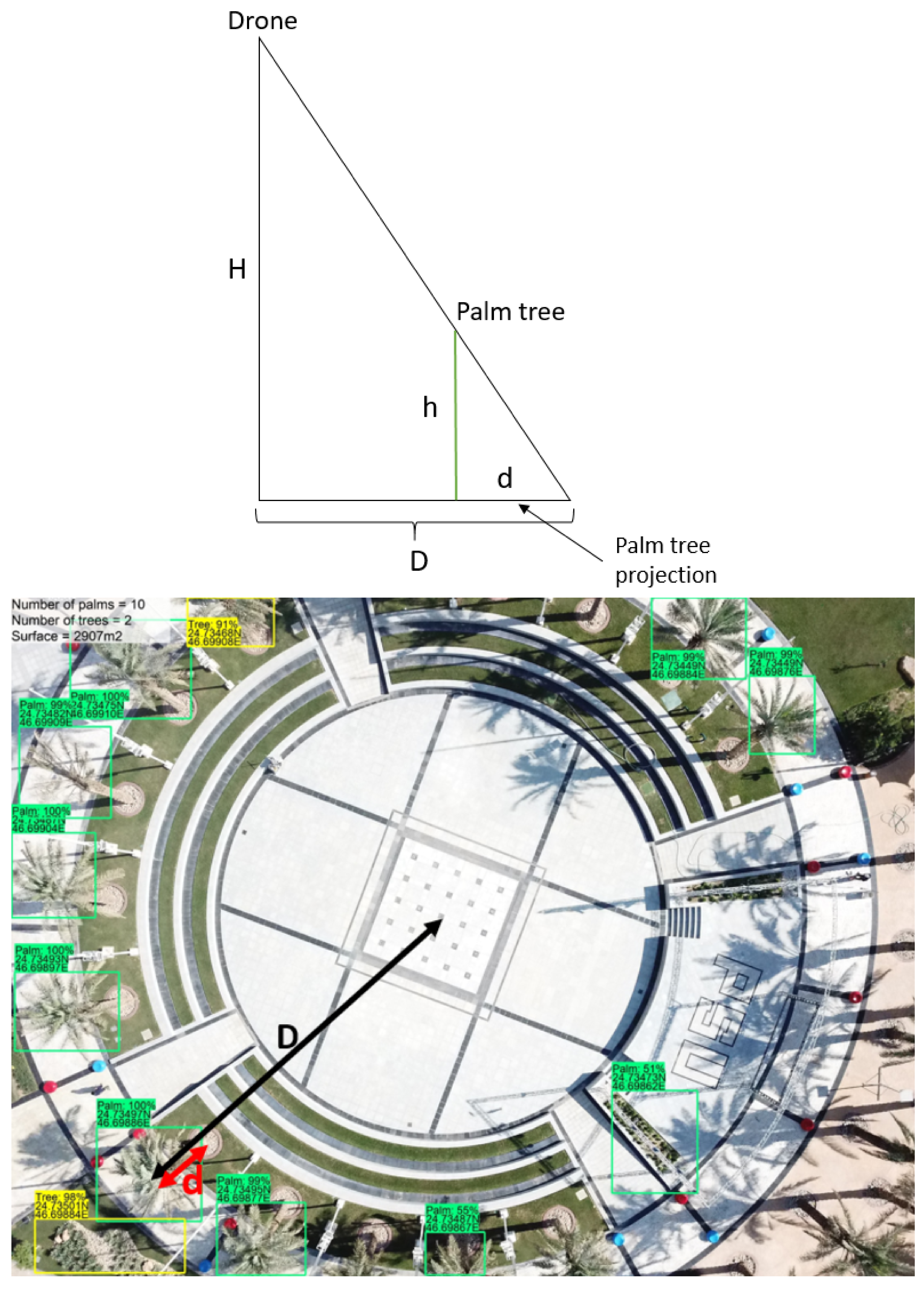
2.5.1. Calculation of the Distance to Image Center

To geolocate a pixel ($x,y$) in a drone image, we first calculate the equivalent distance coordinates to the central pixel ($x_c,y_c$) in the image frame:

$$\left\{\begin{array}{c}{d}_x=\frac{(x-x_c)}{F_x}H\hfill \\ d_y=\frac{(y_c-y)}{F_y}H\hfill \end{array}\right.$$

(5)

where H is the drone altitude, and $F_x$ and $F_y$ represent the calibrated focal length of the camera (in pixels) for width and height and are generally equal.

If the calibrated focal length is unavailable in the metadata of the images, we calculate it from the camera standard focal length as follows:

$$\left\{\begin{array}{c}{F}_x=\frac{I_w{F}_l}{S_x}\hfill \\ F_y=\frac{I_h{F}_l}{S_y}\hfill \end{array}\right.$$

(6)

where $I_w$ and $I_h$ are the image width and height, respectively; $S_x$ and $S_y$ are the CCD sensor width and height, respectively; and $F_l$ is the camera focal length.

Then, we apply a rotation by the value of the flight yaw angle $\psi$ (also available in the image metadata) to convert the image coordinates $(d_x,d_y)$ to local tangent plane (LTP) coordinates $(D_x,D_y)$:

$$\left\{\begin{array}{c}{D}_x=d_{x}cos\left(\psi \right)-d_{y}sin\left(\psi \right)\hfill \\ D_y=d_{x}sin\left(\psi \right)+d_{y}cos\left(\psi \right)\hfill \end{array}\right.$$

(7)

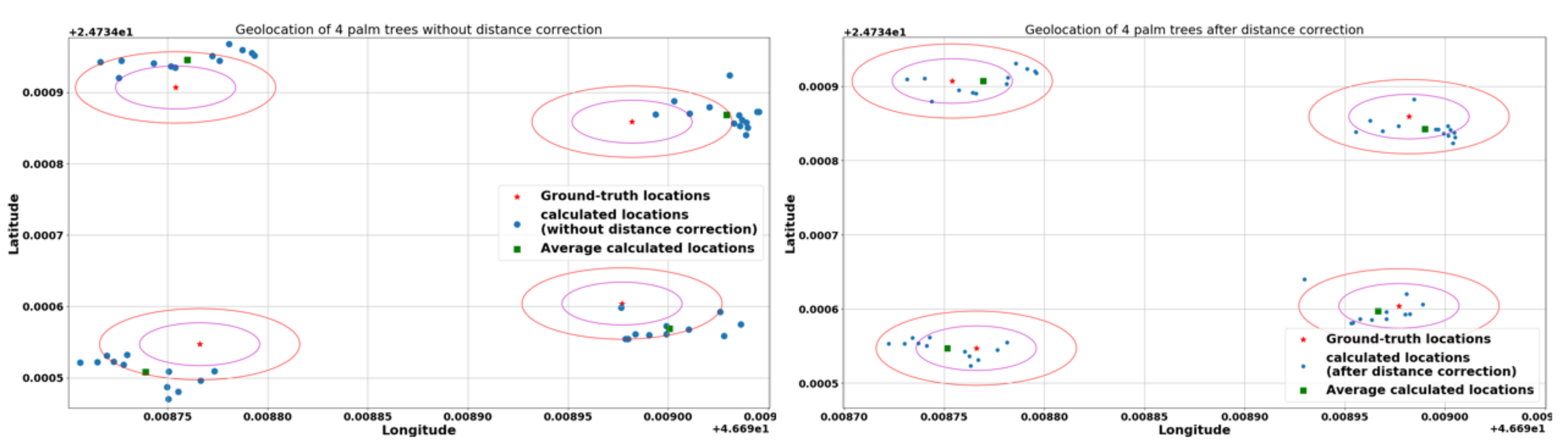
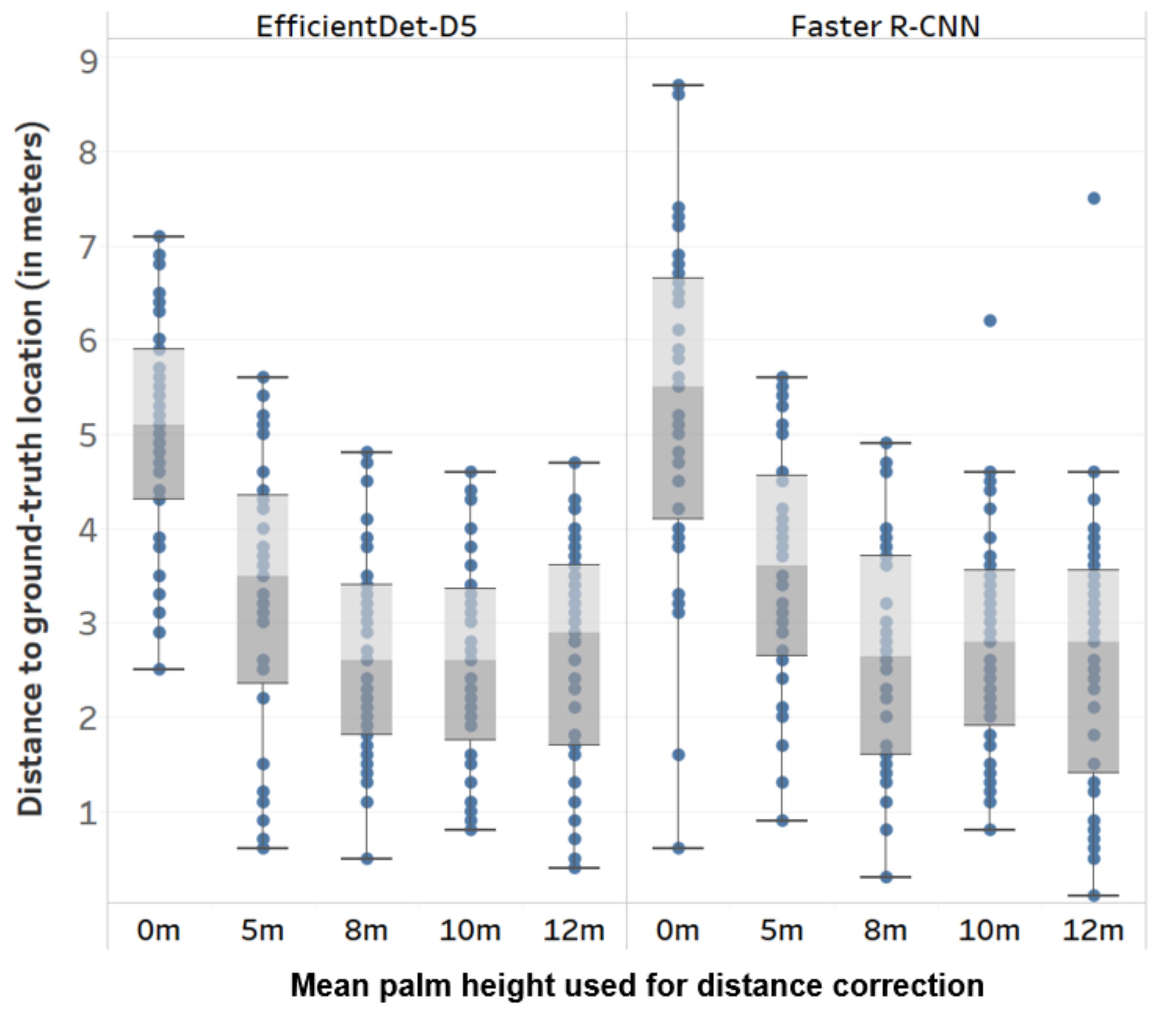
2.5.2. Distance Correction

The locations calculated using (7) still present a bias, as illustrated in Figure 1. This figure shows the calculated detections of palm trees on the PSU campus from images of the same scene (slightly larger than in Figure 2) captured at different altitudes (four images at 41 m, five images at 51 m, five images at 60 m, and six images at 80 m) and different yaw angles. We observe that the calculated locations are all placed on the same side (farther than the ground-truth location with respect to the drone position). This is because the center of the detected bounding corresponds typically to the tree’s summit, which, when projected on the image, appears farther than the tree’s footprint.

Therefore, in order to enhance the geolocation precision and rectify the bias, we apply a distance correction based on an estimation of the average palm tree height. We need this correction to take account of projection issues that induce a difference between the palm tree summit’s position on the image (which corresponds to the center of the detected bounding box) and its footprint. We need to subtract the palm tree projection distance d from the distance D between the center of the detected bounding box (corresponding to the palm tree’s summit) and the center of the image. Using similar triangles rules (Figure 2), we have

$$d=\frac{h}{H}D$$

(8)

where h is the average palm tree height, H is the drone altitude, and $D=\sqrt{d_x^2+d_y^2}$.

Hence, the corrected coordinates are

$$\left\{\begin{array}{c}{D}_x^c=D_x\left(\frac{D-d}{D}\right)\hfill \\ D_y^c=D_y\left(\frac{D-d}{D}\right)\hfill \end{array}\right.$$

(9)

In Section 3.3, we will evaluate the impact of the value of the average palm tree height on the geolocation accuracy.

2.5.3. Conversion to GPS Coordinates

To obtain the GPS coordinates of each detected tree, we convert the distance coordinates calculated in (9) to latitude and longitude degrees using geodesic formulas based on the WGS-84 reference system [46]. Then, we add these converted coordinates to the latitude and longitude of the image center, which correspond to the drone’s GPS location and are extracted from the image metadata. Algorithm 1 summarizes the steps of the whole procedure of inference detection and geolocation.

Algorithm 1 Palm detection and geolocation.

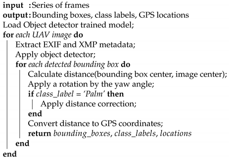3. Experiments

3.1. Datasets

We collected a dataset of 258 aerial images in a palm tree farm in Kharj region, in Saudi Arabia, and 91 images taken on Prince Sultan University campus. A sample of each is shown in Figure 3. Both the aspect and density of palm trees in the two sets of images are dissimilar. The images were captured using two different drones: a DJI Phantom 4 Pro drone equipped with a DJI FC6310 camera (resolutions 4864 × 3648 and 4096 × 2160) and a DJI Mavic Pro equipped with a DJI FC220 camera (resolution 4000 × 3000). The dataset contains a total of 13,071 instances (11,150 palms and 1921 other trees) that we manually labeled using Labelbox [47]. Then we randomly split it into training (80%) and testing (20%) datasets.

Table 1. Number of images and instances in the training and testing datasets.

	Training Dataset	Testing Dataset
Number of images	279	70
Percentage	80%	20%
Instances of class “Palm tree”	8805	2345
Instances of class “Other tree”	1596	325

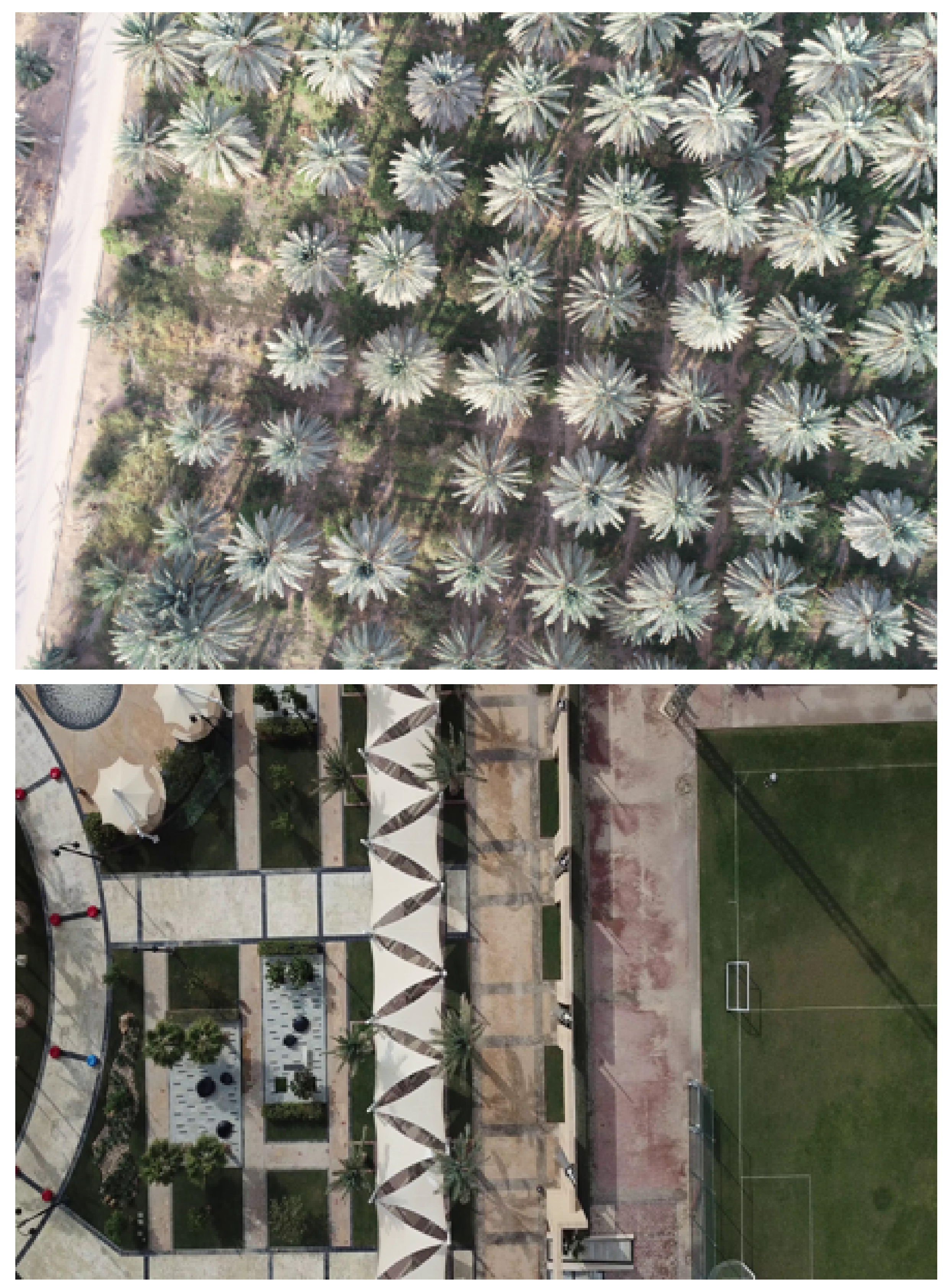
presents the number of images and instances of each class in the training and testing datasets.

3.2. Object Detection

3.2.1. Experimental Setup

The experiments were conducted on a workstation powered by an Intel core i9-9900K (3.6 GHz) processor with 64GB RAM and an NVIDIA GeForce RTX 2080Ti (11 GB) GPU, running on Ubuntu 16.04 LTS.

We trained the four object detectors described in Section 2 (YOLOv3, YOLOv4, EfficientDet-D5, and Faster R-CNN) on the same training dataset described above.

Table 2. Hyperparameters and details of each object detector.

Object Detector	Feature Extractor	Input Size	Number of Parameters	FLOPS	Learning Rate	Batch Size	Number of Steps	Code Repository
Faster R-CNN	Resnet-50	- Conserves the aspect ratio of the original image. - Either the smallest dimension is 600, or the largest dimension is 1024.	3.4 × 10${}^7$	64 G	3 × 10${}^{-5}$	1	30,000	github.com/tensorflow/models/tree/master/research/object_detection Accessed on 21/07/2021
YOLO v3	Darknet-53	608 × 608	6.2 × 10${}^7$	139 G	1 × 10${}^{-4}$	64	30,000	github.com/AlexeyAB/darknet Accessed on 21/07/2021
YOLO v4	CSPDarknet-53	608 × 608	6.4 × 10${}^7$	127 G	1 × 10${}^{-3}$	64	1400	github.com/AlexeyAB/darknet Accessed on 21/07/2021
EfficientDet-D5	EfficientNet-B5	1280 × 1280	3.4 × 10${}^7$	135 G	1 × 10${}^{-4}$	4	30,000	github.com/xuannianz/EfficientDet Accessed on 21/07/2021

records the details of each algorithm. We have chosen EfficientDet-D5 among the family of EfficientDet object detectors because its computational complexity is equivalent to the three other chosen object detectors (especially YOLOv3 and YOLOv4). In fact, EfficientDet-D4 needs only 55 GFLOPS, whereas EfficientDet-D6 necessitates 226 GFLOPS [44]. Faster R-CNN uses a variable input size that conserves the aspect ratio of original images, while the three other algorithms use a fixed square input size. Due to the variable input size, the batch size for Faster R-CNN is required to be 1. For the other three algorithms, the batch size is only limited by the GPU memory capacity. We trained each network for the number of iterations necessary for its convergence. YOLOv4 needed only 1400 steps to converge, while the three other algorithms necessitated 30,000 steps. The fast convergence of YOLOv4 is due to its use of the cosine annealing scheduler [29,36].

3.2.2. Metrics

We have adopted the following widely used metrics [48] to compare the performance of the four object detectors:

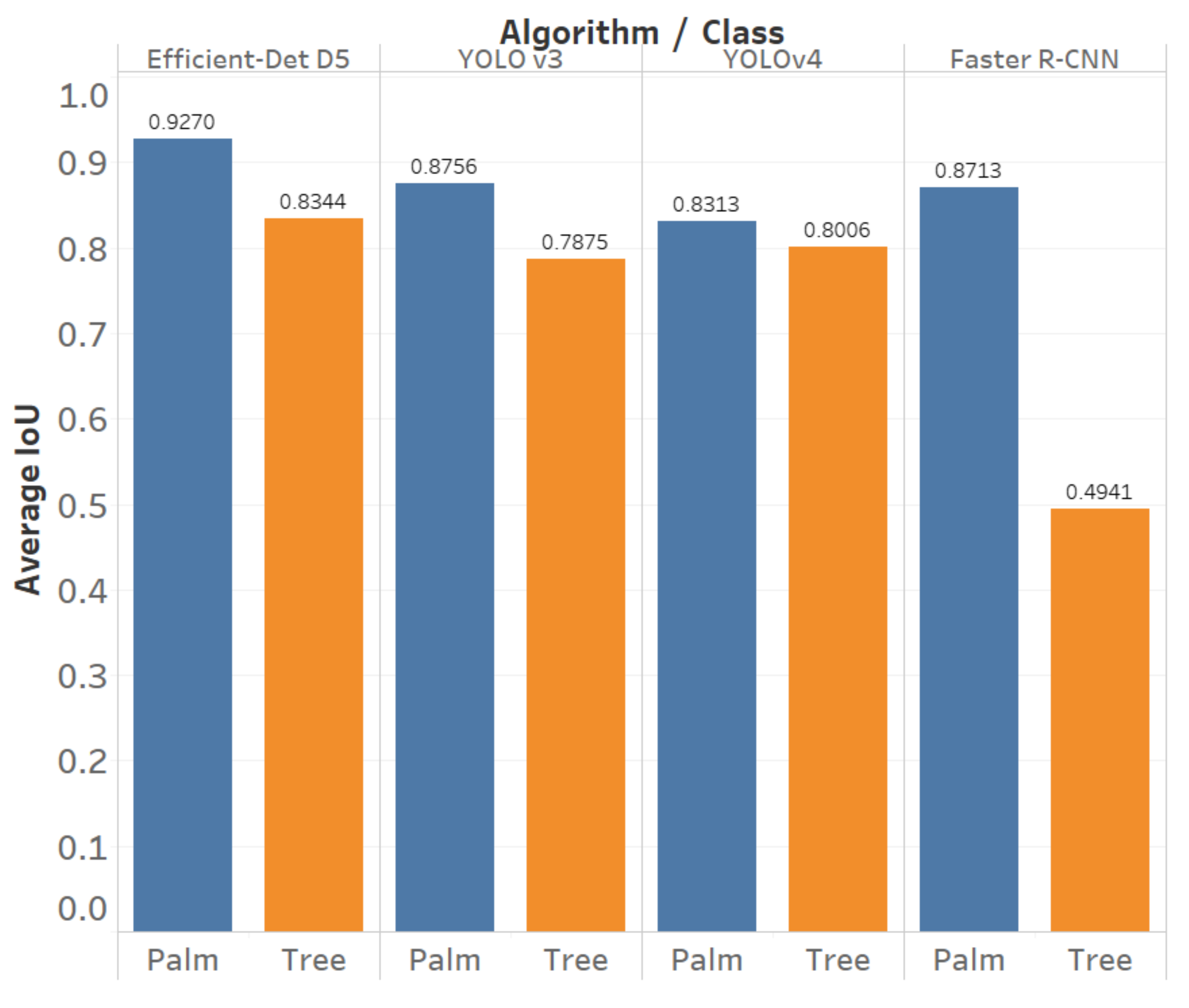
• IoU: intersection over union. It measures the overlap between the predicted ($B_{det}$) and the ground-truth ($B_{gt}$) bounding boxes by dividing the area of their intersection by the area of their union:

  $$\begin{array}{c}IoU=\frac{Area(B_{det}\cap B_{gt})}{Area(B_{det}\cup B_{gt})}\end{array}$$

  (10)
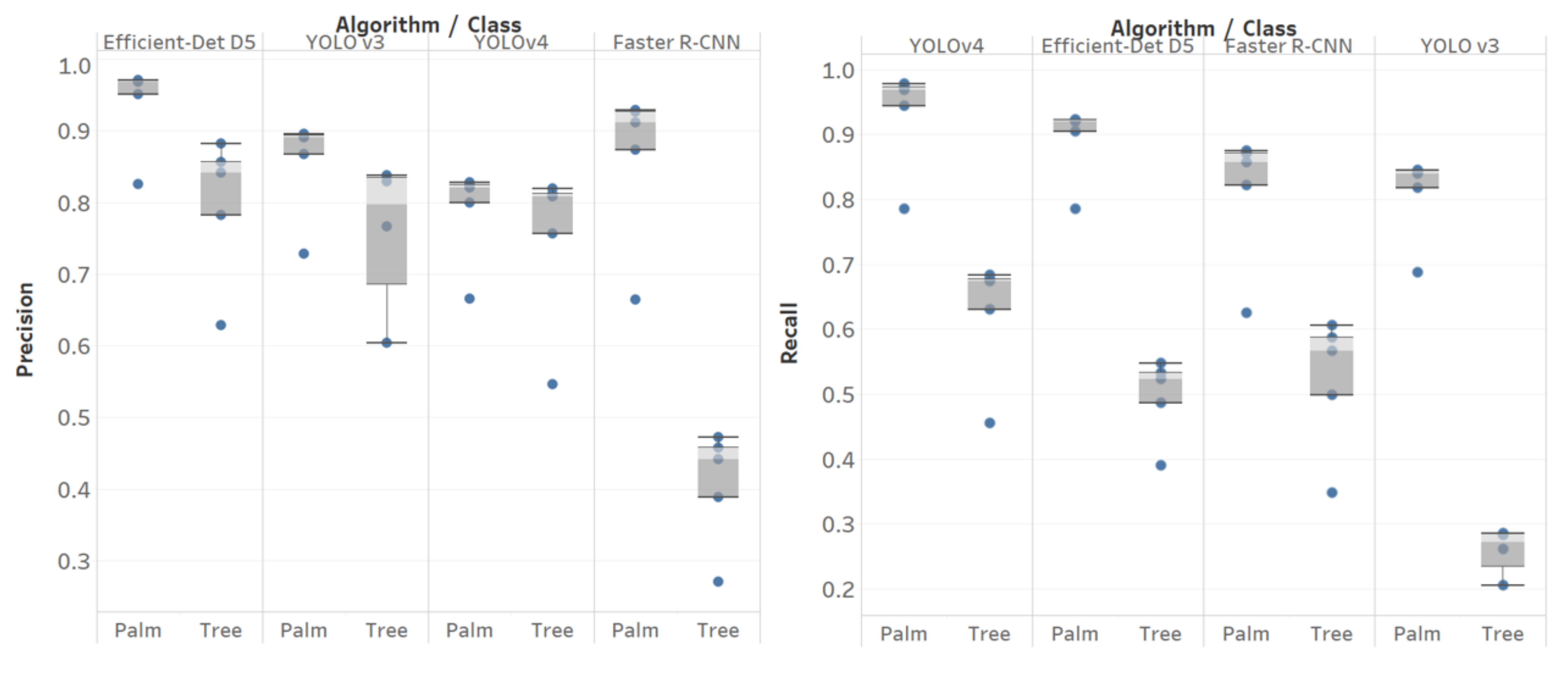
• Precision: ratio of true positives (TP) over all detections (true positives and false positives (FP)).

  $$Precision=\frac{TP}{TP+FP}$$
• Recall: ratio of true positives over the number of relevant objects (true positives and false negatives (FN)).

  $$Recall=\frac{TP}{TP+FN}$$
• F1 score: harmonic mean of precision and recall.

  $$F1=2·\frac{Precision·Recall}{Precision+Recall}$$
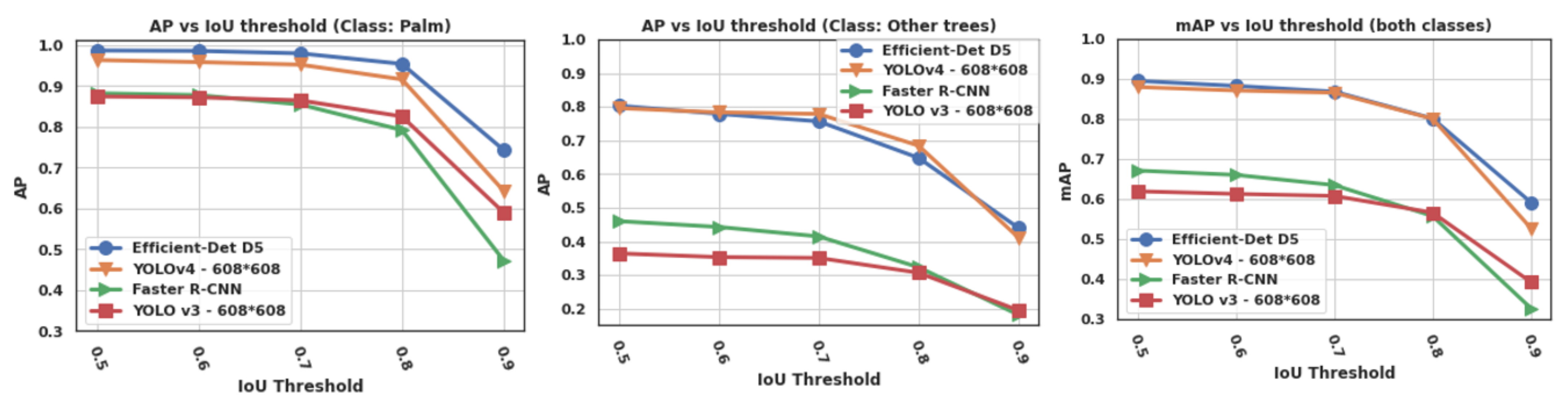
• AP: average precision for one class. It is an approximation of the area under the precision vs. recall curve (AUC). AP was measured for different values of IoU thresholds (0.5, 0.6, 0.7, 0.8, and 0.9).
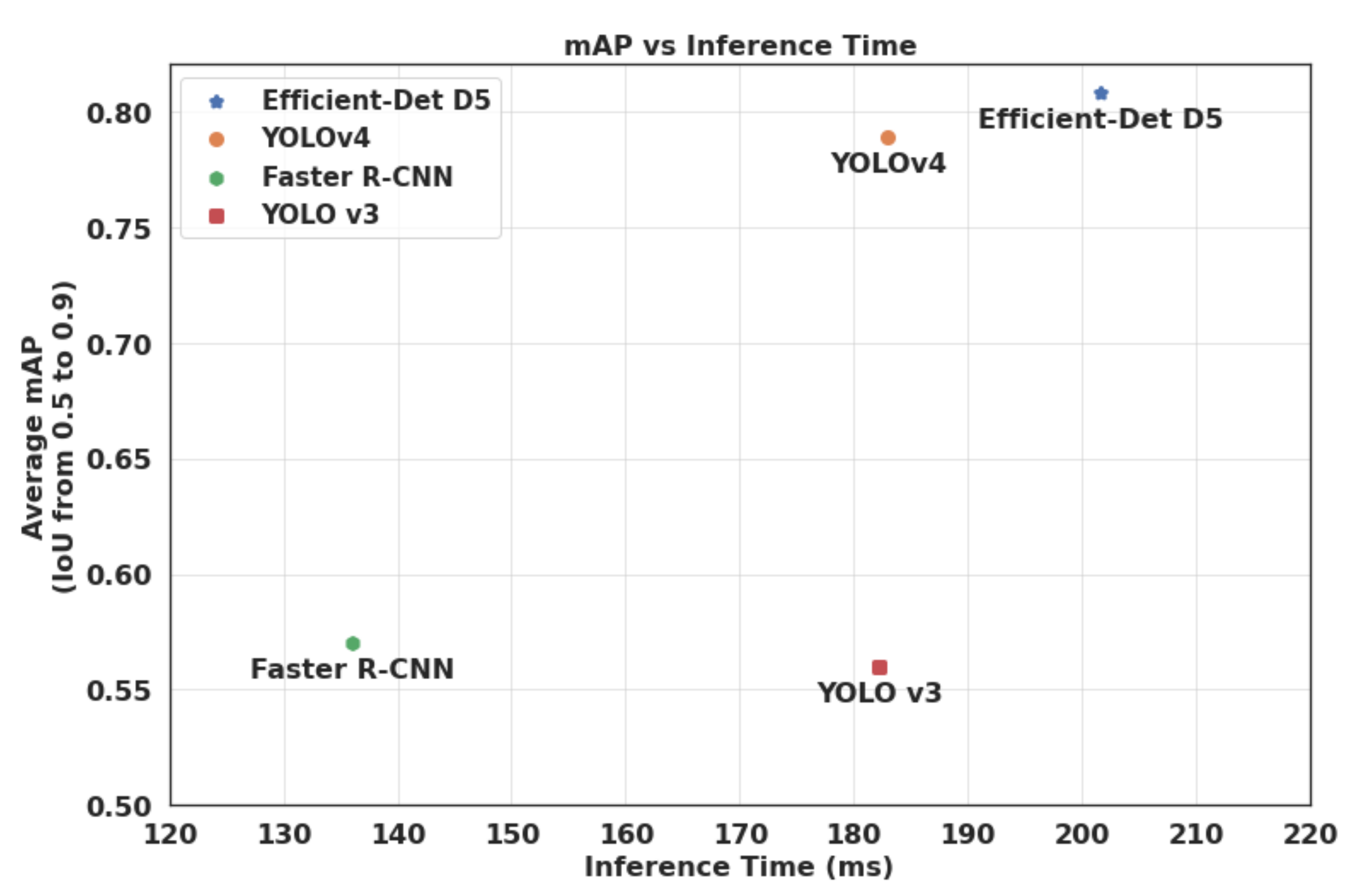
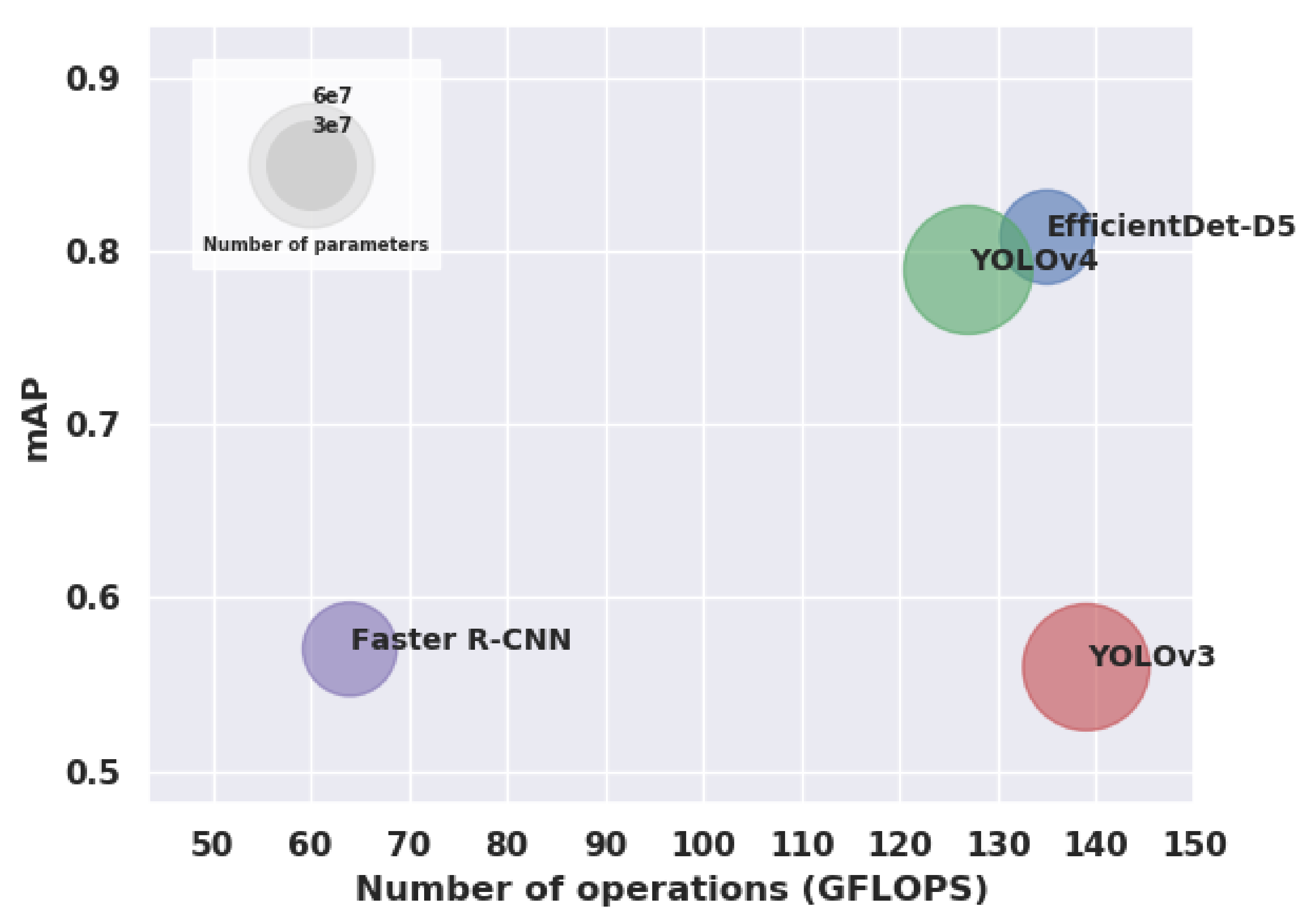
• mAP: mean average precision over the two classes. The mAP is the main metric used for evaluating object detectors [48].
• Inference time (in millisecond per image): it measures the average inference processing time per image.

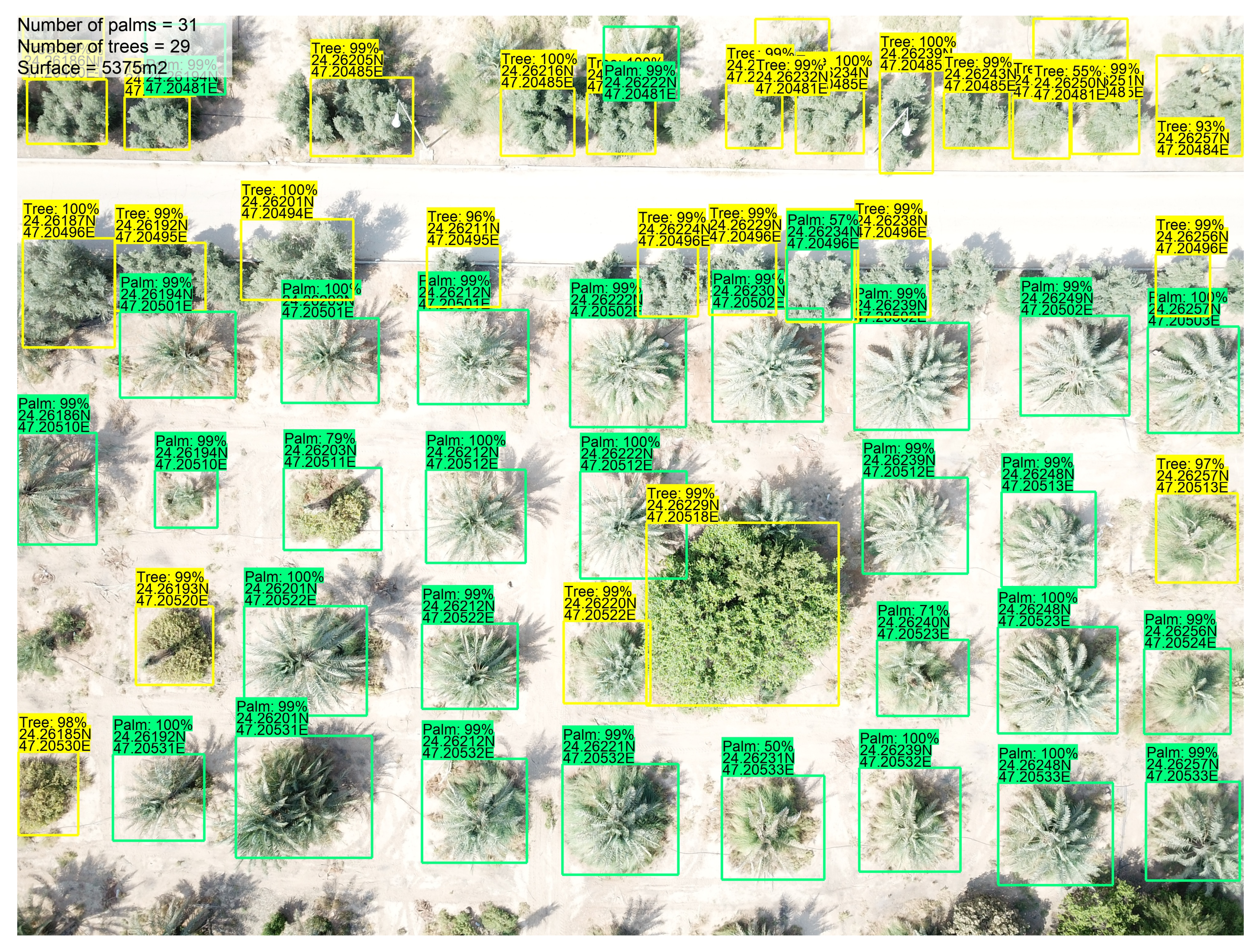
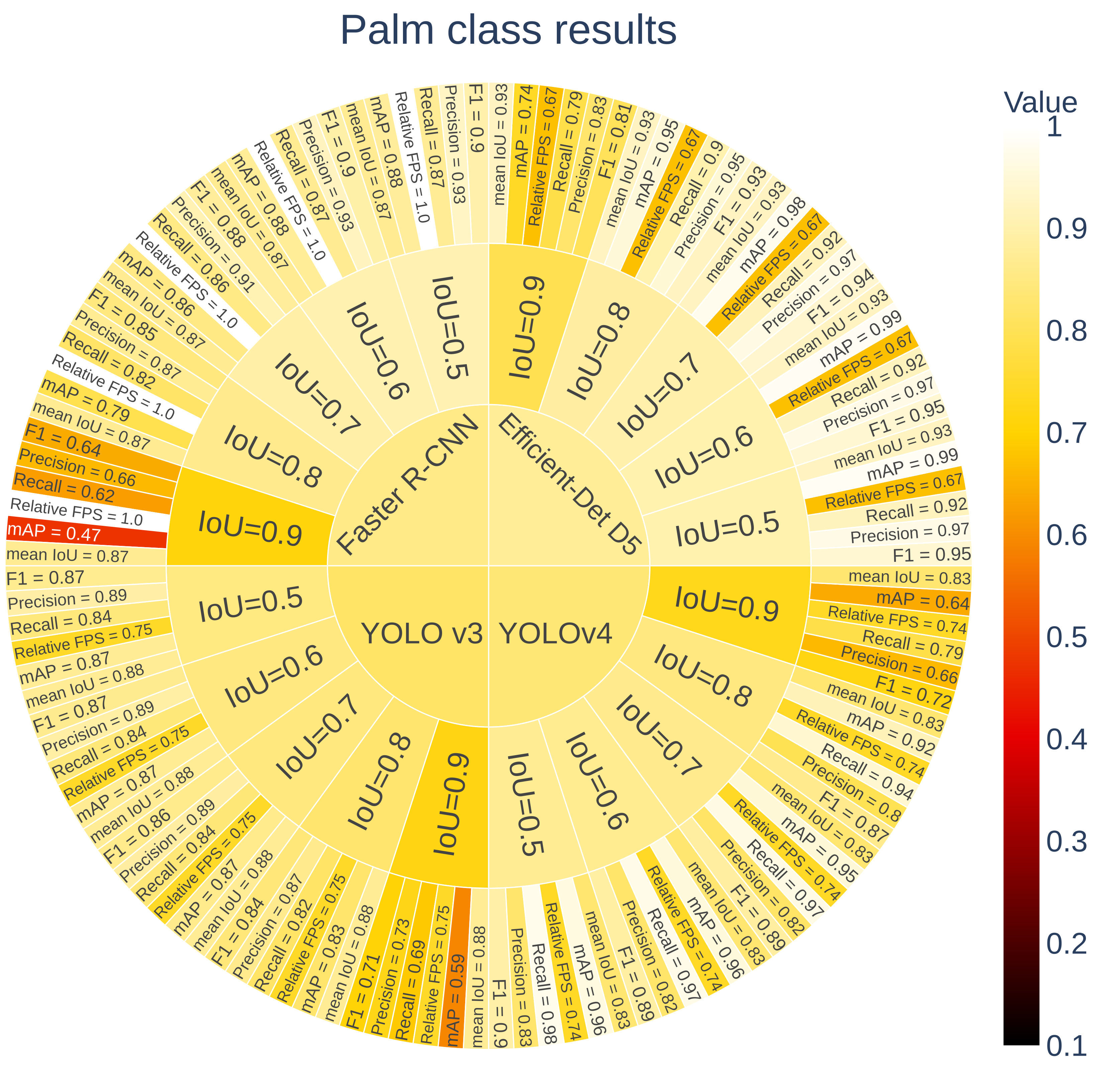
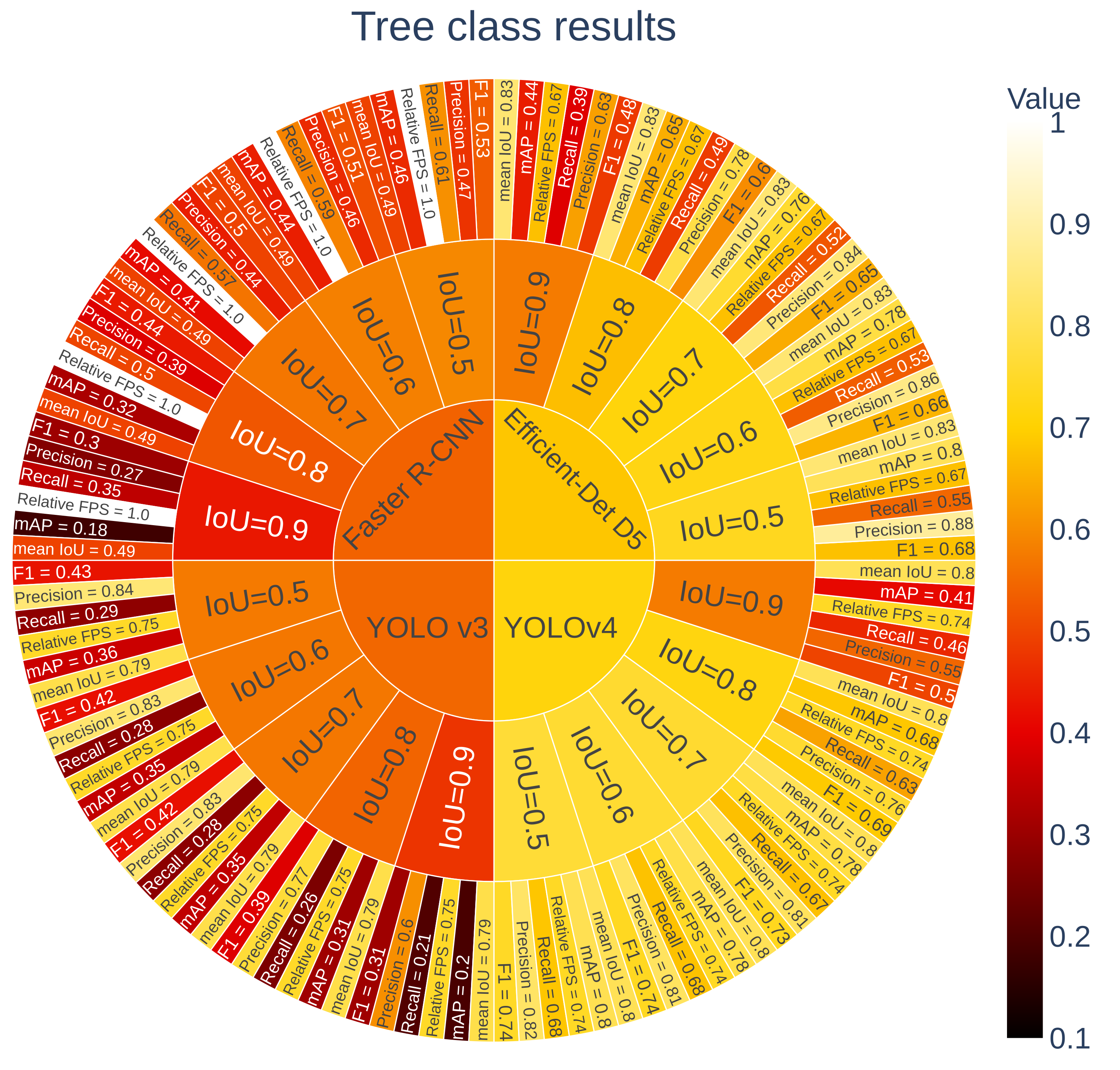
3.2.3. Results

Figure 4 compares the average precision (AP) of the four tested object detectors at different intersection over union (IoU) threshold values for each of the two classes (Palm, and other trees) and the mean average precision (mAP) for both classes. EfficientDet-D5 and YOLOv4 show close results with a slight advantage for the first, and both show significantly higher mAP than Faster R-CNN and YOLOv3. The gap is especially large for the class of other trees, for which Faster R-CNN and YOLOv3 perform poorly (AP lower than 0.5). The better performance of all algorithms on the Palm class is due to the larger number of instances of this class in the training dataset compared to instances of other trees (5.5 times more, as can be seen in Table 1).

Figure 5 depicts the box plots of the precision and recall for each object detector and each class for different values of IoU. EfficientDet-D5 yields the highest precision, while Faster R-CNN yields the lowest with a large gap between the two classes. On the other hand, YOLOv4 shows the highest recall, while YOLOv3 shows the lowest, also with a large disparity between the two classes. The lowest points for both precision and recall figures correspond to an IoU threshold of 0.9 and are extremely distinct from the other points (except for the recall of YOLOv3 on class ‘Tree’, for which all values are already very low). This highlights the fact that all algorithms fall short of providing highly precise bounding boxes.

Figure 6 compares the four algorithms in the mAP/time space. While EfficientDet-D5 shows the best mAP (2.4% higher than the second-best YOLOv4), this comes at the cost of a significantly lower inference speed (10% slower than YOLOv4, and 48% slower than Faster R-CNN). YOLOv4 appears as a good trade-off between mAP and inference speed. While its speed is equivalent to YOLOv3’s (only 0.4% faster), it provides 41% better mAP. Faster R-CNN is the fastest by far, due to its reduced number of operations (Table 2) while yielding an mAP slightly better than YOLOv3. Figure 7 shows a similar plot by substituting the inference time for the number of floating operations, which is independent of the platform and the implementation framework. It confirms that EfficientDet and YOLOv4 have very close performance and that YOLOv3 is relatively inefficient both in terms of number of operations and mAP.

Figure 8 compares the average IoU for each object detector and each class. This metric is of paramount significance for geolocation since the precision of the detected bounding box impacts the precision of the tree’s calculated GPS location. For this metric, we observe that EfficientDet-D5 significantly outperforms the three other algorithms that show close results, except that Faster R-CNN has a remarkably degraded bounding box precision on the ‘other trees’ class. All algorithms show a lower precision on this class, but the gap is notably amplified for Faster R-CNN.

3.2.4. Discussion

Figure 9 and Figure 10 summarize the results of the four object detectors for different IoU thresholds (from 0.5 to 0.9) on the ‘Palm’ and ‘Other trees’ classes, respectively. We observe a large gap between the two classes in all cases, except for the inference speed (relative FPS), which does not depend on the class of detected objects nor the IoU threshold. This gap is more pronounced for Faster R-CNN and YOLOv3 than for EfficientDet-D5 and YOLOv4. The mean IoU is calculated for all detected bounding boxes and is unrelated to the fixed IoU threshold. On the ‘Palm’ class, EfficientDet-D5 shows the best overall results, while on the ‘Other trees’ class, YOLOv4 shows slightly higher performance, which indicates its ability to better deal with classes that are underrepresented in the training dataset.

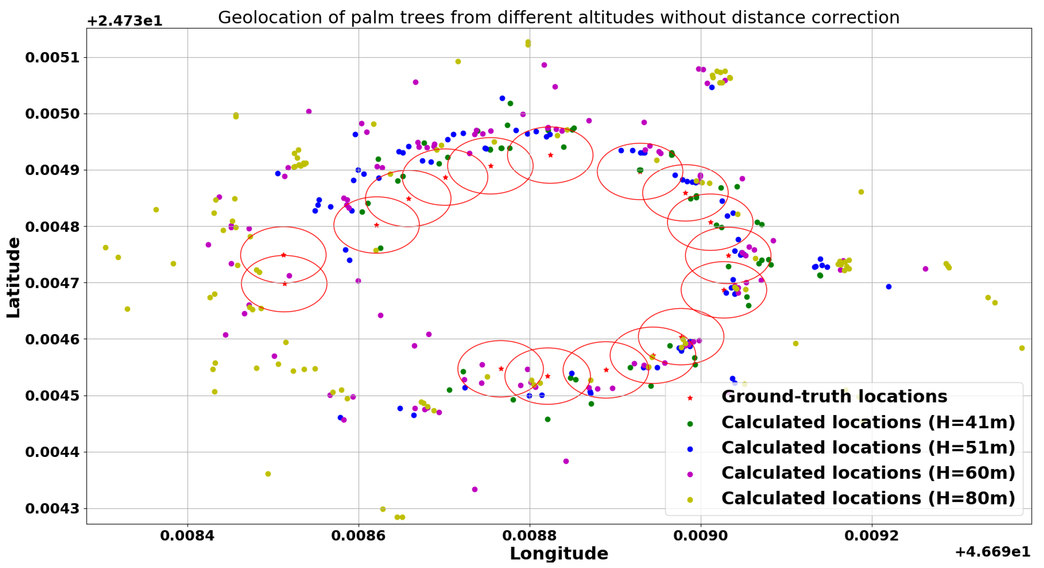
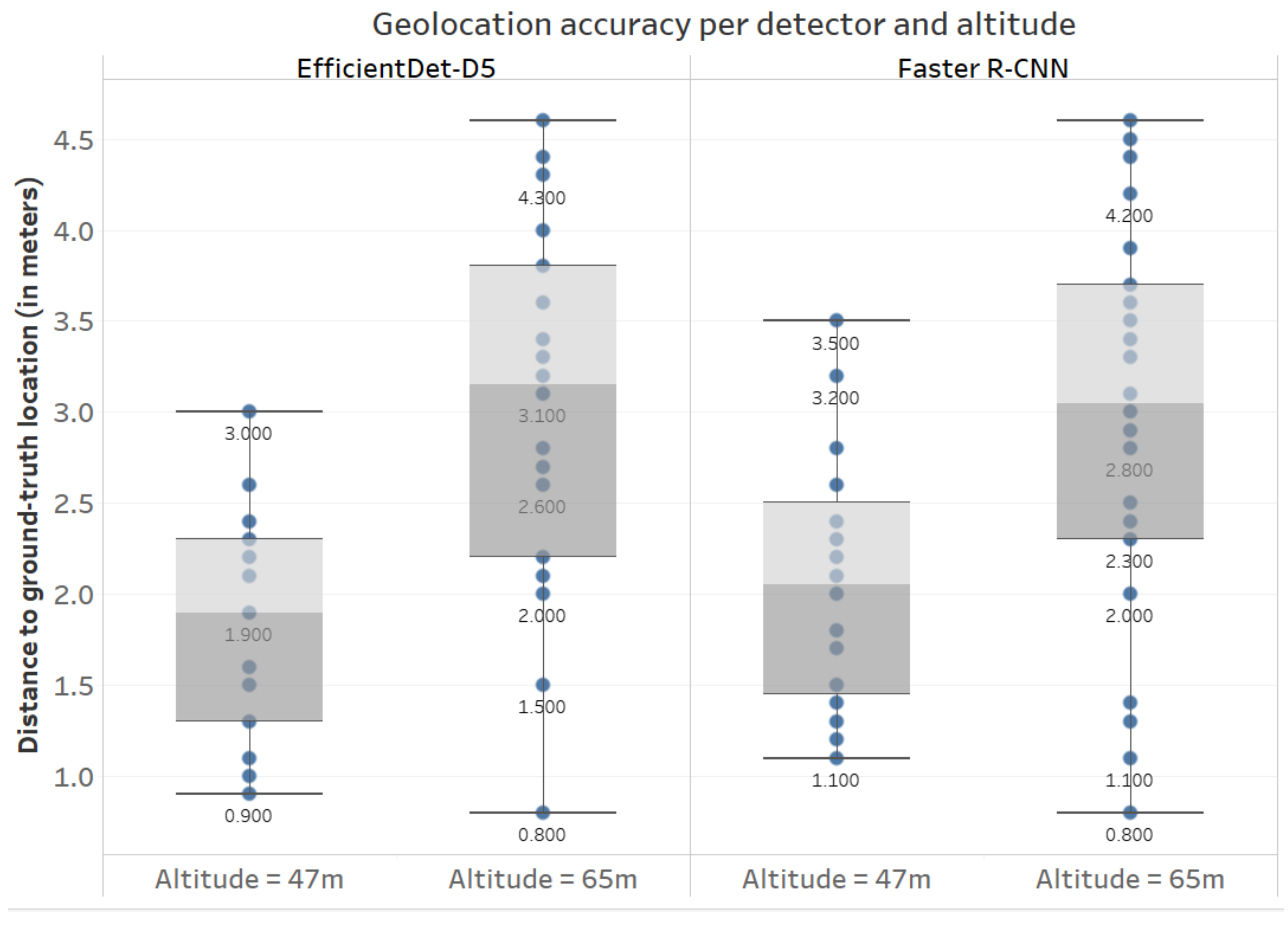
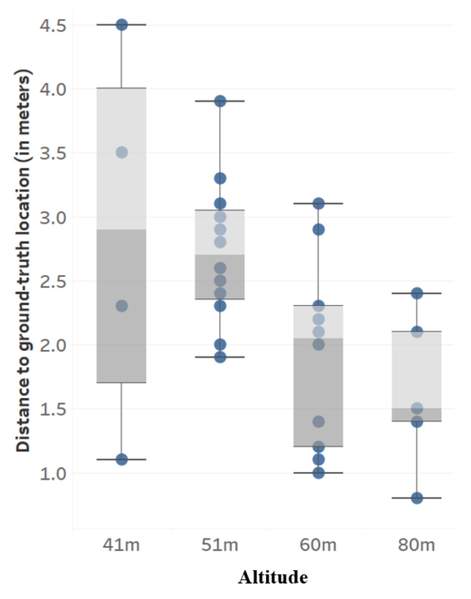
3.3. Geolocation Accuracy

For assessing the geolocation of palm trees, we tested two of the aforementioned object detectors, namely EfficientDet-D5 (which was proven in Section 3.2 to be the most accurate) and Faster R-CNN (which is the least accurate), in order to measure the impact of detection imprecisions on geolocation accuracy. The metric used for assessing the geolocation accuracy is the average distance between the predicted and ground truth locations in meters. After processing a series of UAV images with each object detector, we applied the geolocation process detailed in Section 2.5 to each bounding box center corresponding to the ‘Palm’ class. Figure 11 and Figure 12 show examples of palm detection and geolocation in a UAV image from Al-Kharj farm and the PSU campus, respectively. They display on top of each detected bounding box the class of the object (palm tree or other tree), the classification confidence level, and the latitude and longitude of the bounding box center. Palm identifiers are also displayed (inside the bounding boxes) for some selected palm trees. This automatic identification was determined by comparing the calculated locations of detected bounding box centers to predefined locations of 17 palm trees on the PSU campus measured in situ.

figure at the top of each detected bounding box (in green for palm and yellow for other trees): the class name, the confidence level, the latitude, and the longitude. At the top left are shown: the number of palms, the number of other trees, and the surface covered by the image.

Figure 13 shows an original UAV image of palms on the PSU campus (right) and four sufficiently spaced palms (left), with a minimum distance of 21 m separating them. The remaining parts of the left image were hidden in order to obtain only four detections and facilitate the matching between detected and real palms for performance assessment. We used 15 such images that show only these same four palm trees to assess the accuracy of their calculated geolocation. The matching is done by comparing the calculated location to the location measured in situ by the drone placed at ground level. The 15 images used for testing were captured by a DJI Mavic Pro drone from different altitudes (between 33 m and 65 m) and yaw degrees (between −148${}^{\circ }$ and 163${}^{\circ }$), while the gimbal pitch angle was kept fixed at 90${}^{\circ }$.

Figure 14 compares the calculated locations of the four selected palms (ID = 1, 5, 9, and 12 in

Table 3. Real height (measured in situ) of 17 selected palm trees organized in a circle on PSU campus (see Figure 12).

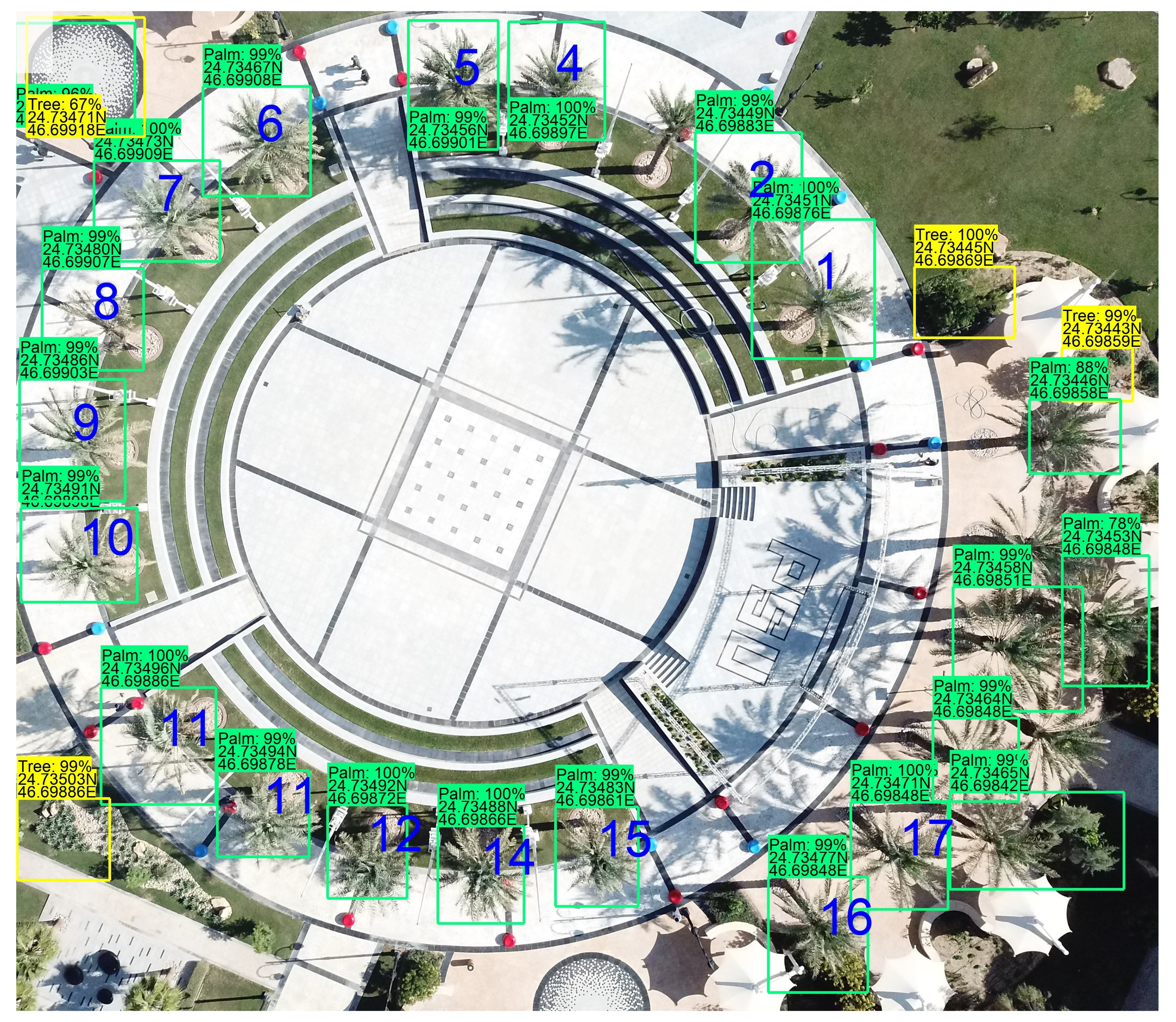
Palm ID	1	2	3	4	5	6	7	8	9	10	11	12	13	14	15	16	17
Height (in meters)	15	14	14	13	13	11	8.3	8.3	9.1	8.9	10	10.1	11	10.5	9.8	8.4	8.1

and Figure 12) before and after the distance correction explained in Section 2.5.2. Before the distance correction, all calculated detections are on the same side (farther than the ground-truth location with respect to the drone location) so that the bias cannot be eliminated by averaging. In contrast, after the distance correction (with an average palm height fixed at 10 m), the bias is remarkably reduced, most calculated detections are within 5 m of ground-truth locations, and the average calculated location is within less than 3 m.

More precisely, Figure 15 depicts the box plot of the accuracy of our geolocation method, after detection with Faster R-CNN and EfficientDet-D5, for different values of mean palm height used for correction. We notice a considerable improvement in accuracy when using distance correction. For both object detectors, the best accuracy is obtained when we fix the average palm height at 10 m, which roughly corresponds to the actual mean height of date palm trees [49], even though the palm trees in the dataset have variable heights. The average accuracy in this case, when using Faster R-CNN, is 2.7 m, with a standard deviation of 1.1 m. When we use the EfficientDet-D5 object detector, we obtain a similar accuracy of 2.6 m on average, with a standard deviation of 1.1 m, which shows that the geolocation process is not very sensitive to the type of object detector used once we apply a suitable distance correction. It is also lowly sensitive to the average palm height parameter when it is in the 8 to 12 m range (Figure 15), which corresponds to the height of most palm trees in the dataset. Furthermore, the four palm trees (ID = 1, 5, 9, and 12) that we selected for testing have variable heights ranging from 9 m to 15 m, but this did not significantly affect the geolocation accuracy, as can be seen in Figure 14. This means that a rough estimation of the mean average height of the surveyed palm trees is sufficient. This average height for distance correction can either be approximated by manually measuring the height of a few representative palm trees from the farm to be surveyed or measured using depth sensors such as LIDAR that could be embedded on the drone.

The geolocation accuracy also depends on the drone’s relative altitude. Figure 16 compares the box plots of distances to ground-truth locations for images captured at two different altitudes when using distance correction based on a mean palm height of 10 m for both EfficientDet-D5 and Faster R-CNN detectors. At an altitude of 47 m, our method’s average accuracy when using EfficientDet-D5 attains 1.8 m (2.1 m for Faster R-CNN) with a standard deviation of 0.7 m (same for Faster R-CNN), while at 65 m, the Faster R-CNN results are slightly better, showing an average accuracy of 3.0 m with a standard deviation of 1.1 m, against an average of 3.2 m and a standard deviation of 0.9 m for EfficientDet-D5. These results indicate that Faster R-CNN performs better on smaller objects. Conversely, the geolocation accuracy does not show any significant dependency on the flight yaw angle.

In order to assess the impact of the camera type, we tested the same geolocation technique on images captured by a Phantom 4 Pro equipped with a DJI FC6310 camera (resolution 4864 × 3648). Figure 17 depicts the geolocation accuracy obtained for different relative altitudes. Compared to the results obtained with the Mavic Pro DJI FC220 camera (Figure 16), we observe that the altitude has an inverse effect on the geolocation accuracy, which ranges from an average of 2.9 m at 41 m down to 1.6 m at 80 m. This is likely due to the higher resolution of the FC6310 camera and the better vertical view angle.

In order not to confuse the detected palm trees, the distance error needs to be lower than half the distance between neighbor trees. The average distance between neighboring palm trees in our dataset is around 9 m, which means that the accuracy of our geolocalization technique meets the requirements.

4. Conclusions

We presented a deep learning system that automatically detects and geolocates palm trees from UAV images using convolutional neural networks. After collecting a dataset of palm trees from two different regions in Saudi Arabia, we analyzed and compared the performance of four recent convolutional neural network models. YOLOv4 and EfficientDet-D5 yielded the best trade-off between accuracy and speed, while Faster R-CNN and YOLOv3 were significantly less accurate, but with a large advantage for the former in terms of speed.

In a second phase, we applied photogrammetry concepts and distance corrections to the UAV images’ geotagged metadata to automatically determine the geographical location of detected palm trees. This geolocation technique was assessed to provide an average geolocation accuracy that attains 1.6 m at an altitude of 80 m and to be lowly sensitive to the object detector type. This GPS tagging technique uniquely identifies palm trees, facilitating their counting from a series of overlapping drone images. Furthermore, we can generalize this technique to any other objects in UAV images after adapting the average height parameter used for distance correction. Nevertheless, the detection accuracy should first be assessed, as the features may be harder to discern, such as in the case of a uniform canopy, with a high degree of occlusion such that individual trees may not be accurately delimited. In future works, we intend to apply this method for tree counting in large geographical regions. We should then evaluate the percentage of error caused by image overlapping and compare the accuracy of this approach to existing counting techniques (e.g., manual counting or those based on satellite imagery.

References

- Otero, V.; Van De Kerchove, R.; Satyanarayana, B.; Martínez-Espinosa, C.; Fisol, M.A.B.; Ibrahim, M.R.B.; Sulong, I.; Mohd-Lokman, H.; Lucas, R.; Dahdouh-Guebas, F. Managing mangrove forests from the sky: Forest inventory using field data and Unmanned Aerial Vehicle (UAV) imagery in the Matang Mangrove Forest Reserve, peninsular Malaysia. For. Ecol. Manag. 2018, 411, 35–45. [Google Scholar] [CrossRef]
- Yue, J.; Yang, G.; Li, C.; Li, Z.; Wang, Y.; Feng, H.; Xu, B. Estimation of winter wheat above-ground biomass using unmanned aerial vehicle-based snapshot hyperspectral sensor and crop height improved models. Remote Sens. 2017, 9, 708. [Google Scholar] [CrossRef] [Green Version]
- Caruso, G.; Zarco-Tejada, P.J.; González-Dugo, V.; Moriondo, M.; Tozzini, L.; Palai, G.; Rallo, G.; Hornero, A.; Primicerio, J.; Gucci, R. High-resolution imagery acquired from an unmanned platform to estimate biophysical and geometrical parameters of olive trees under different irrigation regimes. PLoS ONE 2019, 14, e0210804. [Google Scholar] [CrossRef] [Green Version]
- Shahbazi, M.; Théau, J.; Ménard, P. Recent applications of unmanned aerial imagery in natural resource management. GIScience Remote Sens. 2014, 51, 339–365. [Google Scholar] [CrossRef]
- Kaartinen, H.; Hyyppä, J. EuroSDR/ISPRS Project Commission II, Tree Extraction; Final Report; EuroSDR: Dublin, Ireland, 2008; pp. 1–60. [Google Scholar]
- Kaartinen, H.; Hyyppä, J.; Yu, X.; Vastaranta, M.; Hyyppä, H.; Kukko, A.; Holopainen, M.; Heipke, C.; Hirschmugl, M.; Morsdorf, F.; et al. An International Comparison of Individual Tree Detection and Extraction Using Airborne Laser Scanning. Remote Sens. 2012, 4, 950–974. [Google Scholar] [CrossRef] [Green Version]
- FAOSTAT Crop Statistics. Available online: http://www.fao.org/faostat/en/ (accessed on 24 November 2020).
- Yao, S.; Al-Redhaiman, K. Date Palm Cultivation in Saudi Arabia: Current Status and Future Prospects for Development. In Proceedings of the ASHS Annual Conference, Orlando, FL, USA, 28–31 July 2014; Volume 49, pp. 139–140. [Google Scholar]
- Shafri, H.Z.M.; Hamdan, N.; Saripan, M.I. Semi-automatic detection and counting of oil palm trees from high spatial resolution airborne imagery. Int. J. Remote Sens. 2011, 32, 2095–2115. [Google Scholar] [CrossRef]
- Bazi, Y.; Malek, S.; Alajlan, N.; AlHichri, H. An automatic approach for palm tree counting in UAV images. In Proceedings of the 2014 IEEE Geoscience and Remote Sensing Symposium, Quebec City, QC, Canada, 13–18 July 2014; pp. 537–540. [Google Scholar] [CrossRef]
- Li, W.; Fu, H.; Yu, L.; Cracknell, A. Deep Learning Based Oil Palm Tree Detection and Counting for High-Resolution Remote Sensing Images. Remote Sens. 2016, 9, 22. [Google Scholar] [CrossRef] [Green Version]
- Li, W.; Fu, H.; Yu, L. Deep convolutional neural network based large-scale oil palm tree detection for high-resolution remote sensing images. In Proceedings of the 2017 IEEE International Geoscience and Remote Sensing Symposium (IGARSS), Fort Worth, TX, USA, 23–28 July 2017; pp. 846–849. [Google Scholar] [CrossRef]
- Zheng, J.; Fu, H.; Li, W.; Wu, W.; Zhao, Y.; Dong, R.; Yu, L. Cross-regional oil palm tree counting and detection via a multi-level attention domain adaptation network. ISPRS J. Photogramm. Remote Sens. 2020, 167, 154–177. [Google Scholar] [CrossRef]
- Zheng, J.; Fu, H.; Li, W.; Wu, W.; Yu, L.; Yuan, S.; Tao, W.Y.W.; Pang, T.K.; Kanniah, K.D. Growing status observation for oil palm trees using Unmanned Aerial Vehicle (UAV) images. ISPRS J. Photogramm. Remote Sens. 2021, 173, 95–121. [Google Scholar] [CrossRef]
- Yarak, K.; Witayangkurn, A.; Kritiyutanont, K.; Arunplod, C.; Shibasaki, R. Oil Palm Tree Detection and Health Classification on High-Resolution Imagery Using Deep Learning. Agriculture 2021, 11, 183. [Google Scholar] [CrossRef]
- Zortea, M.; Nery, M.; Ruga, B.; Carvalho, L.B.; Bastos, A.C. Oil-Palm Tree Detection in Aerial Images Combining Deep Learning Classifiers. In Proceedings of the IGARSS 2018—2018 IEEE International Geoscience and Remote Sensing Symposium, Valencia, Spain, 22–27 July 2018; pp. 657–660. [Google Scholar] [CrossRef]
- Mansour, S.; Chockalingam, J. Diagnostically counting palm date trees in Al-Ahssa Governorate of Saudi Arabia: An integrated GIS and remote sensing processing of IKONOS imagery. Spat. Inf. Res. 2020, 28, 579–588. [Google Scholar] [CrossRef]
- Neupane, B.; Horanont, T.; Hung, N.D. Deep learning based banana plant detection and counting using high-resolution red-green-blue (RGB) images collected from unmanned aerial vehicle (UAV). PLoS ONE 2019, 14, e0223906. [Google Scholar] [CrossRef]
- Ioffe, S.; Szegedy, C. Batch Normalization: Accelerating Deep Network Training by Reducing Internal Covariate Shift. arXiv 2015, arXiv:1502.03167. [Google Scholar]
- Song, S.; Jing, J.; Huang, Y.; Shi, M. EfficientDet for fabric defect detection based on edge computing. J. Eng. Fibers Fabr. 2021, 16. [Google Scholar] [CrossRef]
- Liao, J.; Zou, J.; Shen, A.; Liu, J.; Du, X. Cigarette end detection based on EfficientDet. In Journal of Physics: Conference Series; IOP Publishing: Bristol, UK, 2021; Volume 1748, p. 062015. [Google Scholar]
- Wu, D.; Lv, S.; Jiang, M.; Song, H. Using channel pruning-based YOLO v4 deep learning algorithm for the real-time and accurate detection of apple flowers in natural environments. Comput. Electron. Agric. 2020, 178, 105742. [Google Scholar] [CrossRef]
- Ammar, A.; Koubaa, A.; Ahmed, M.; Saad, A.; Benjdira, B. Vehicle detection from aerial images using deep learning: A comparative study. Electronics 2021, 10, 820. [Google Scholar] [CrossRef]
- Huang, Y.Q.; Zheng, J.C.; Sun, S.D.; Yang, C.F.; Liu, J. Optimized YOLOv3 algorithm and its application in traffic flow detections. Appl. Sci. 2020, 10, 3079. [Google Scholar] [CrossRef]
- Hung, J.; Carpenter, A. Applying faster R-CNN for object detection on malaria images. In Proceedings of the IEEE Conference on Computer Vision and Pattern Recognition Workshops, Honolulu, HI, USA, 21–26 July 2017; pp. 56–61. [Google Scholar]
- Redmon, J.; Divvala, S.K.; Girshick, R.B.; Farhadi, A. You Only Look Once: Unified, Real-Time Object Detection. In Proceedings of the 2016 IEEE Conference on Computer Vision and Pattern Recognition (CVPR 2016), Las Vegas, NV, USA, 27–30 June 2016; pp. 779–788. [Google Scholar] [CrossRef] [Green Version]
- Redmon, J.; Farhadi, A. YOLO9000: Better, Faster, Stronger. In Proceedings of the 2017 IEEE Conference on Computer Vision and Pattern Recognition (CVPR 2017), Honolulu, HI, USA, 21–26 July 2017; pp. 6517–6525. [Google Scholar] [CrossRef] [Green Version]
- Redmon, J.; Farhadi, A. YOLOv3: An Incremental Improvement. arXiv 2018, arXiv:1804.02767. [Google Scholar]
- Bochkovskiy, A.; Wang, C.Y.; Liao, H.Y.M. YOLOv4: Optimal Speed and Accuracy of Object Detection. arXiv 2020, arXiv:2004.10934. [Google Scholar]
- Lin, T.Y.; Maire, M.; Belongie, S.; Hays, J.; Perona, P.; Ramanan, D.; Dollár, P.; Zitnick, C.L. Microsoft coco: Common objects in context. In European Conference on Computer Vision; Springer: Berlin/Heidelberg, Germany, 2014; pp. 740–755. [Google Scholar]
- Yun, S.; Han, D.; Chun, S.; Oh, S.J.; Yoo, Y.; Choe, J. CutMix: Regularization Strategy to Train Strong Classifiers With Localizable Features. In Proceedings of the 2019 IEEE/CVF International Conference on Computer Vision (ICCV), Seoul, Korea, 27 October–3 November 2019; pp. 6023–6032. [Google Scholar] [CrossRef] [Green Version]
- Ghiasi, G.; Lin, T.Y.; Le, Q.V. DropBlock: A regularization method for convolutional networks. arXiv 2018, arXiv:1810.12890. [Google Scholar]
- Szegedy, C.; Vanhoucke, V.; Ioffe, S.; Shlens, J.; Wojna, Z. Rethinking the Inception Architecture for Computer Vision. In Proceedings of the 2016 IEEE Conference on Computer Vision and Pattern Recognition (CVPR), Las Vegas, NV, USA, 27–30 June 2016. [Google Scholar] [CrossRef] [Green Version]
- Zheng, Z.; Wang, P.; Liu, W.; Li, J.; Ye, R.; Ren, D. Distance-IoU Loss: Faster and Better Learning for Bounding Box Regression. arXiv 2019, arXiv:1911.08287. [Google Scholar] [CrossRef]
- Yao, Z.; Cao, Y.; Zheng, S.; Huang, G.; Lin, S. Cross-Iteration Batch Normalization. arXiv 2020, arXiv:2002.05712. [Google Scholar]
- Loshchilov, I.; Hutter, F. SGDR: Stochastic Gradient Descent with Warm Restarts. arXiv 2016, arXiv:1608.03983. [Google Scholar]
- Misra, D. Mish: A Self Regularized Non-Monotonic Neural Activation Function. arXiv 2019, arXiv:1908.08681. [Google Scholar]
- Wang, C.Y.; Liao, H.Y.M.; Yeh, I.H.; Wu, Y.H.; Chen, P.Y.; Hsieh, J.W. CSPNet: A New Backbone that can Enhance Learning Capability of CNN. arXiv 2019, arXiv:1911.11929. [Google Scholar]
- Shen, F.; Gan, R.; Zeng, G. Weighted residuals for very deep networks. In Proceedings of the 2016 3rd International Conference on Systems and Informatics (ICSAI), Shanghai, China, 19–21 November 2016. [Google Scholar] [CrossRef] [Green Version]
- Huang, Z.; Wang, J.; Fu, X.; Yu, T.; Guo, Y.; Wang, R. DC-SPP-YOLO: Dense connection and spatial pyramid pooling based YOLO for object detection. Inf. Sci. 2020, 522, 241–258. [Google Scholar] [CrossRef] [Green Version]
- Ferrari, V.; Hebert, M.; Sminchisescu, C.; Weiss, Y. CBAM: Convolutional Block Attention Module. In Proceedings of the Computer Vision—ECCV 2018; Ferrari, V.; Hebert, M.; Sminchisescu, C.; Weiss, Y. Lecture Notes in Computer Science; Springer: Berlin/Heidelberg, Germany, 2018; Volume 11211, pp. 3–19. [Google Scholar] [CrossRef] [Green Version]
- Liu, S.; Qi, L.; Qin, H.; Shi, J.; Jia, J. Path Aggregation Network for Instance Segmentation. In Proceedings of the 2018 IEEE/CVF Conference on Computer Vision and Pattern Recognition, Salt Lake City, UT, USA, 18–23 June 2018. [Google Scholar] [CrossRef] [Green Version]
- Ren, S.; He, K.; Girshick, R.; Sun, J. Faster R-CNN: Towards Real-Time Object Detection with. IEEE Trans. Pattern Anal. Mach. Intell. 2017, 39, 1137–1149. [Google Scholar] [CrossRef] [Green Version]
- Tan, M.; Pang, R.; Le, Q.V. Efficientdet: Scalable and efficient object detection. arXiv 2019, arXiv:1911.09070. [Google Scholar]
- Tan, M.; Le, Q.V. EfficientNet: Rethinking Model Scaling for Convolutional Neural Networks. arXiv 2020, arXiv:1905.11946. [Google Scholar]
- US National Imagery and Mapping Agency. World Geodetic System 1984, Its Definition and Relationships with Local Geodetic Systems; NIMA Technical Report 8350.2; US National Imagery and Mapping Agency: Fort Belvoir, VA, USA, 1997. [Google Scholar]
- Labelbox. Available online: https://labelbox.com (accessed on 10 February 2020).
- Padilla, R.; Netto, S.L.; da Silva, E.A. A survey on performance metrics for object-detection algorithms. In Proceedings of the 2020 International Conference on Systems, Signals and Image Processing (IWSSIP), Niteroi, Brazil, 1–3 July 2020; pp. 237–242. [Google Scholar]
- Jahromi, M.K.; Jafari, A.; Rafiee, S.; Mohtasebi, S. Survey on some physical properties of the Date Palm tree. J. Agric. Technol. 2007, 3, 317–322. [Google Scholar]