
QVigourMap: A GIS Open Source Application for the Creation of Canopy Vigour Maps


Abstract
1. Introduction
2. Materials and Methods
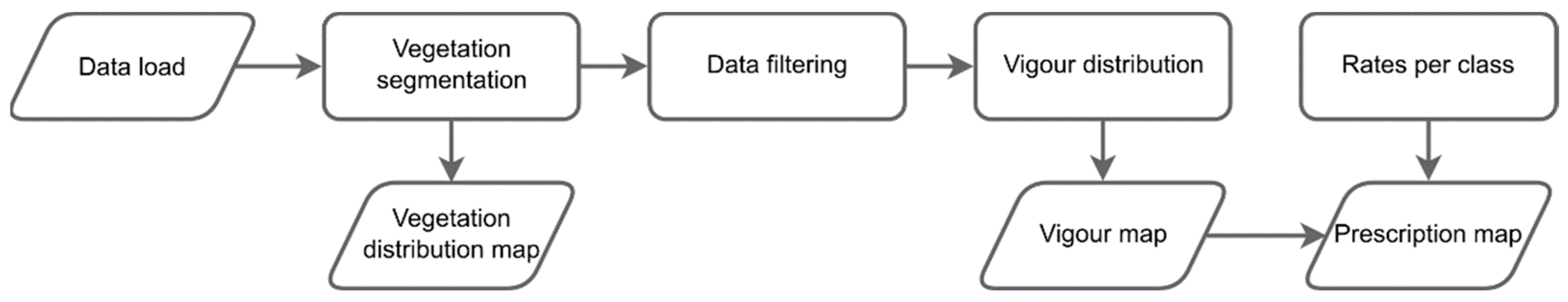
2.1. Methodology
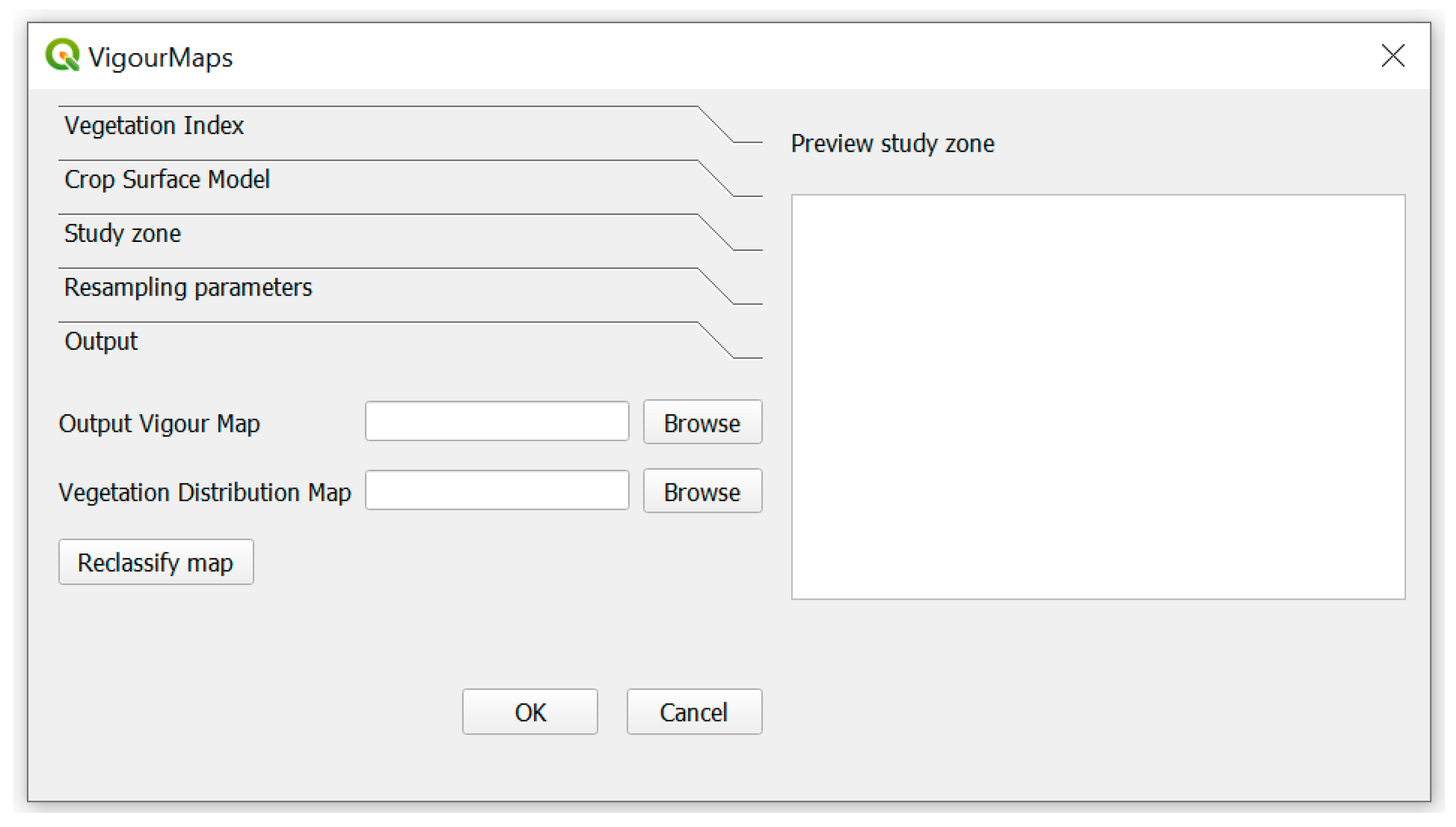
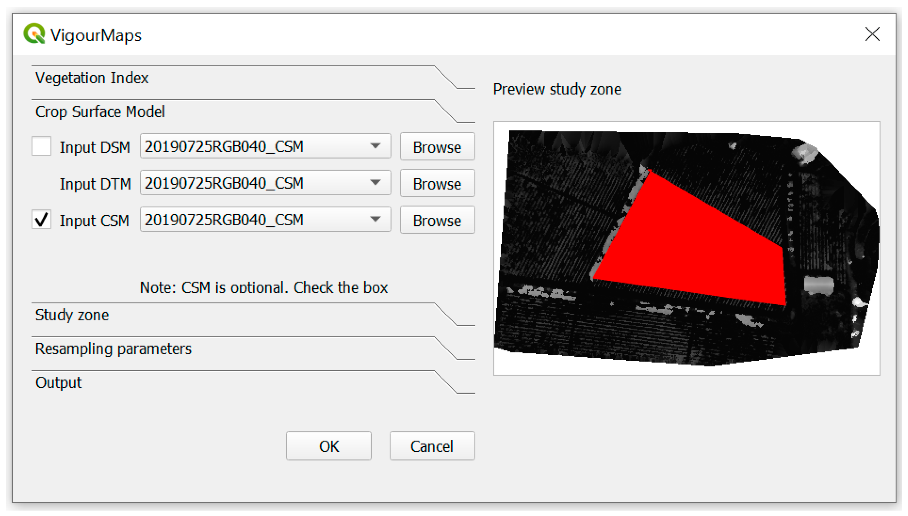
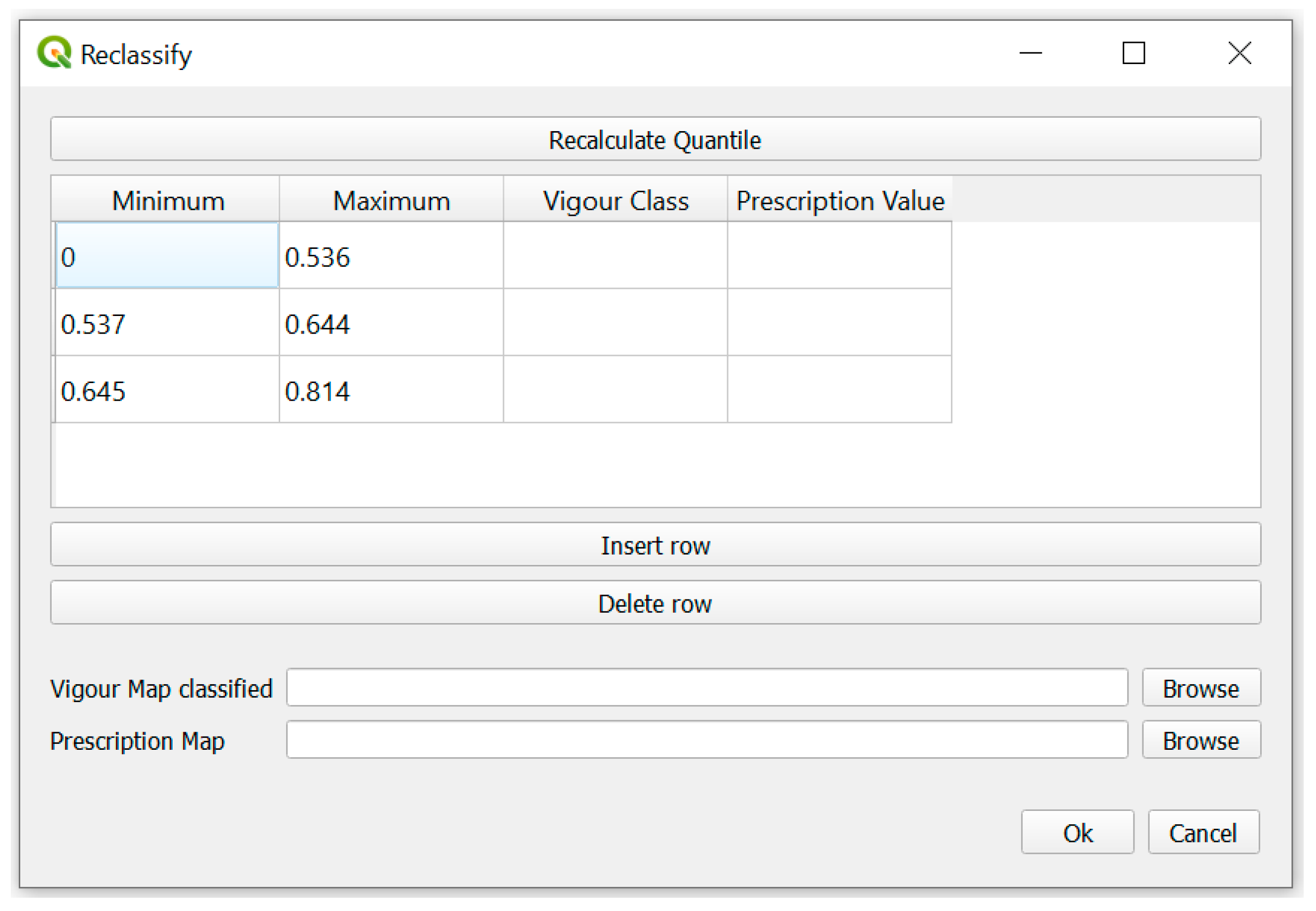
2.2. QVigourMaps Application
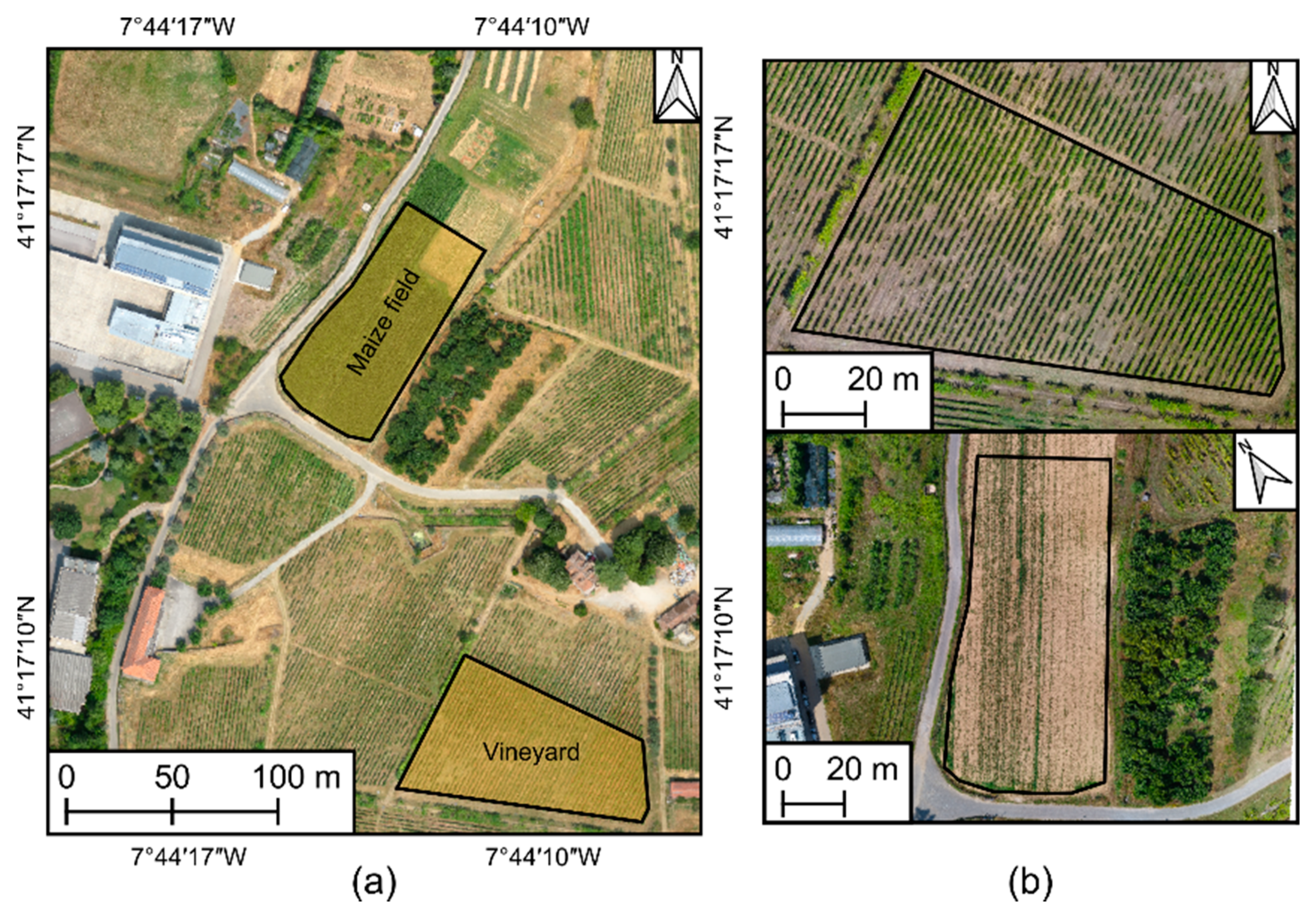
2.3. Case Study
2.3.1. Data Acquisition
2.3.2. Data Processing
3. Experimental Results
3.1. QVigourMap Use Cases
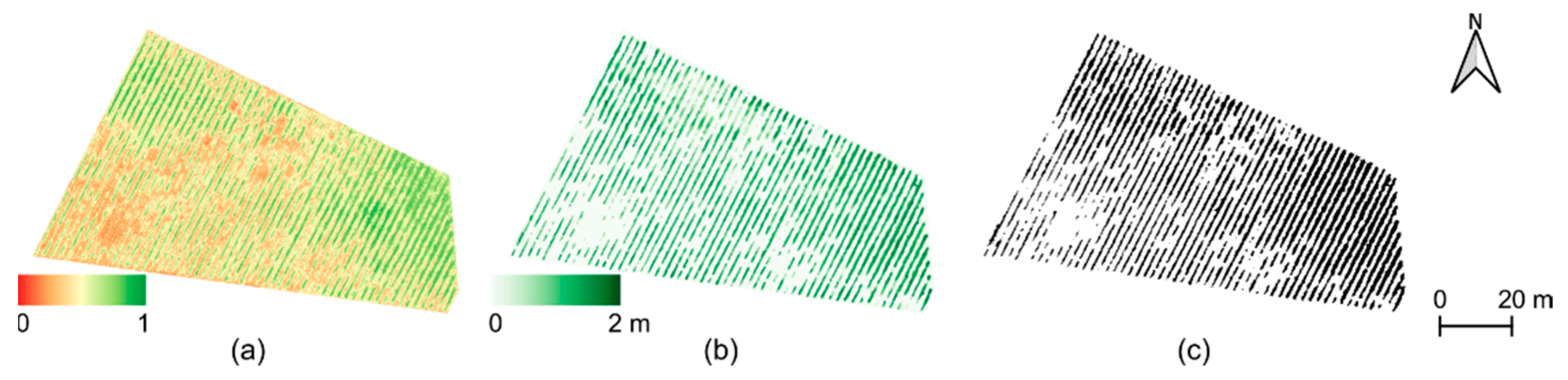
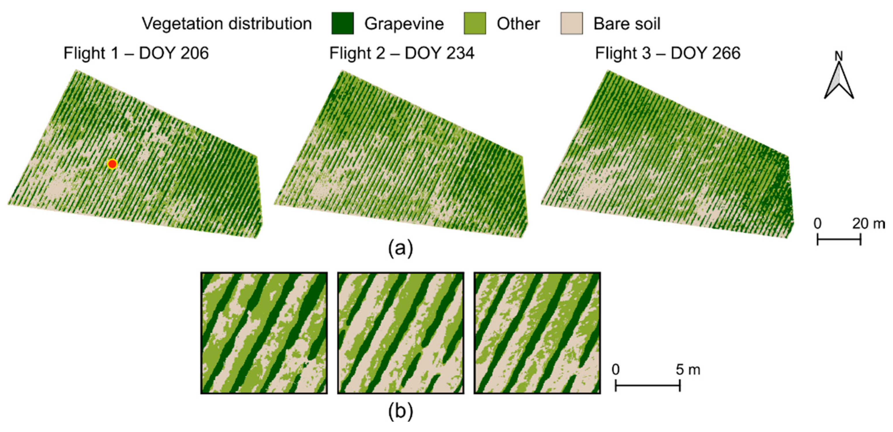
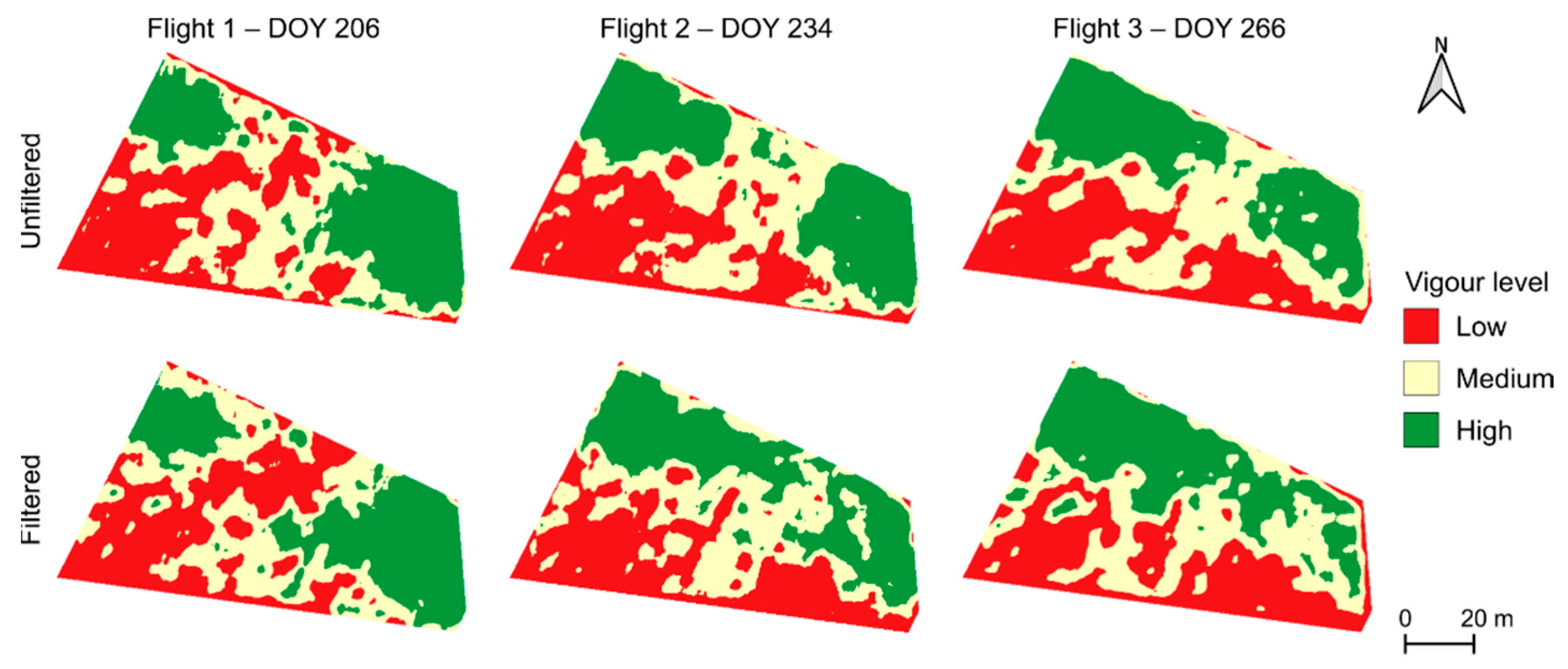
3.1.1. Vineyard
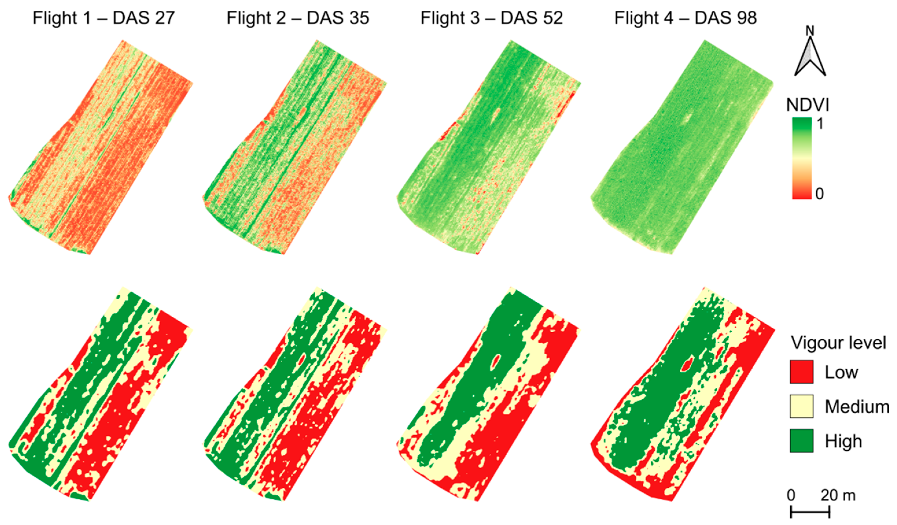
3.1.2. Silage Maize
3.2. Processing Time Performance
4. Discussion and Conclusions
Supplementary Materials
Author Contributions
Funding
Institutional Review Board Statement
Informed Consent Statement
Data Availability Statement
Conflicts of Interest
References
- International Society of Precision Agriculture Precision Ag Definition. Available online: https://www.ispag.org/about/definition (accessed on 1 April 2021).
- Sassu, A.; Gambella, F.; Ghiani, L.; Mercenaro, L.; Caria, M.; Pazzona, A.L. Advances in Unmanned Aerial System Remote Sensing for Precision Viticulture. Sensors 2021, 21, 956. [Google Scholar] [CrossRef]
- Lan, Y.; Thomson, S.J.; Huang, Y.; Hoffmann, W.C.; Zhang, H. Current status and future directions of precision aerial application for site-specific crop management in the USA. Comput. Electron. Agric. 2010, 74, 34–38. [Google Scholar] [CrossRef]
- Lakshmi, V.; Corbett, J. How Artificial Intelligence Improves Agricultural Productivity and Sustainability: A Global Thematic Analysis. 2020. Available online: https://scholarspace.manoa.hawaii.edu/handle/10125/64381 (accessed on 8 May 2021).
- Shendryk, Y.; Davy, R.; Thorburn, P. Integrating satellite imagery and environmental data to predict field-level cane and sugar yields in Australia using machine learning. Field Crops Res. 2021, 260, 107984. [Google Scholar] [CrossRef]
- Bell, S.; Barriocanal, C.; Terrer, C.; Rosell-Melé, A. Management opportunities for soil carbon sequestration following agricultural land abandonment. Environ. Sci. Policy 2020, 108, 104–111. [Google Scholar] [CrossRef]
- Pádua, L.; Vanko, J.; Hruška, J.; Adão, T.; Sousa, J.J.; Peres, E.; Morais, R. UAS, sensors, and data processing in agroforestry: A review towards practical applications. Int. J. Remote Sens. 2017, 38, 2349–2391. [Google Scholar] [CrossRef]
- Campos, J.; Llop, J.; Gallart, M.; García-Ruiz, F.; Gras, A.; Salcedo, R.; Gil, E. Development of canopy vigour maps using UAV for site-specific management during vineyard spraying process. Precis. Agric. 2019. [Google Scholar] [CrossRef]
- Castaldi, F.; Pelosi, F.; Pascucci, S.; Casa, R. Assessing the potential of images from unmanned aerial vehicles (UAV) to support herbicide patch spraying in maize. Precis. Agric. 2017, 18, 76–94. [Google Scholar] [CrossRef]
- López-Granados, F.; Torres-Sánchez, J.; Serrano-Pérez, A.; de Castro, A.I.; Mesas-Carrascosa, F.-J.; Pena, J.-M. Early season weed mapping in sunflower using UAV technology: Variability of herbicide treatment maps against weed thresholds. Precis. Agric. 2016, 17, 183–199. [Google Scholar] [CrossRef]
- Rouse, J.W., Jr.; Haas, R.H.; Schell, J.A.; Deering, D.W. Monitoring Vegetation Systems in The Great Plains with ERTS. In Proceedings of the Goddard Space Flight Center 3d ERTS-1 Symp., NASA, Greenbelt, MD, USA, 1 May 1974; Volume 1, pp. 309–317. [Google Scholar]
- Pádua, L.; Marques, P.; Adão, T.; Guimarães, N.; Sousa, A.; Peres, E.; Sousa, J.J. Vineyard Variability Analysis through UAV-Based Vigour Maps to Assess Climate Change Impacts. Agronomy 2019, 9, 581. [Google Scholar] [CrossRef]
- Richard Stallman Richard Stallman’s Personal Site. Available online: https://stallman.org/ (accessed on 5 April 2021).
- Teodoro, A.C.; Duarte, L. Forest fire risk maps: A GIS open source application–a case study in Norwest of Portugal. Int. J. Geogr. Inf. Sci. 2013, 27, 699–720. [Google Scholar] [CrossRef]
- Duarte, L.; Espinha Marques, J.; Teodoro, A.C. An open source GIS-based application for the assessment of groundwater vulnerability to pollution. Environments 2019, 6, 86. [Google Scholar] [CrossRef]
- Duarte, L.; Teodoro, A.; Gonçalves, J.; Soares, D.; Cunha, M. Assessing soil erosion risk using RUSLE through a GIS open source desktop and web application. Environ. Monit. Assess. 2016, 188, 351. [Google Scholar] [CrossRef] [PubMed]
- Duarte, L.; Teodoro, A.C.; Monteiro, A.T.; Cunha, M.; Gonçalves, H. QPhenoMetrics: An open source software application to assess vegetation phenology metrics. Comput. Electron. Agric. 2018, 148, 82–94. [Google Scholar] [CrossRef]
- Jung, M. LecoS—A python plugin for automated landscape ecology analysis. Ecol. Inform. 2016, 31, 18–21. [Google Scholar] [CrossRef]
- Duarte, L.; Silva, P.; Teodoro, A.C. Development of a QGIS Plugin to Obtain Parameters and Elements of Plantation Trees and Vineyards with Aerial Photographs. ISPRS Int. J. Geo-Inf. 2018, 7, 109. [Google Scholar] [CrossRef]
- Andrade, M.A.; O’Shaughnessy, S.A.; Evett, S.R. ARSPivot, a sensor-based decision support software for variable-rate irrigation center pivot systems: Part A. Development. Trans. ASABE 2020, 63, 1521–1533. [Google Scholar] [CrossRef]
- Huang, Y.; Reddy, K.N.; Fletcher, R.S.; Pennington, D. UAV low-altitude remote sensing for precision weed management. Weed Technol. 2018, 32, 2–6. [Google Scholar] [CrossRef]
- Abbas, A.; Zaman, Q.U.; Schumann, A.W.; Brewster, G.; Donald, R.; Chattha, H.S. Effect of Split Variable Rate Fertilizationon Ammonia Volatilization in Wild Blueberry Cropping System. Appl. Eng. Agric. 2014, 30, 619–627. [Google Scholar]
- QGIS Association. QGIS Geographic Information System. 2021. Available online: https://qgis.org/en/site/ (accessed on 5 April 2021).
- Duarte, L.; Teodoro, A.C.; Moutinho, O.; Gonçalves, J.A. Open-Source GIS Application for UAV Photogrammetry Based on MicMac. Int. J. Remote Sens. 2017, 38, 3181–3202. [Google Scholar] [CrossRef]
- Andrade, M.A.; O’Shaughnessy, S.A.; Evett, S.R. ARSPivot, A Sensor-Based Decision Support Software for Variable-Rate Irrigation Center Pivot Systems: Part B. Application. Trans. ASABE 2020, 63, 1535–1547. [Google Scholar] [CrossRef]
- QGIS Association. QGIS Official Plugins Repository. 2021. Available online: https://plugins.qgis.org/plugins/ (accessed on 5 April 2021).
- Ratcliff, C.; Gobbett, D.; Bramley, R. PAT-Precision Agriculture Tools. V2 CSIRO. Software Collection 2019. Available online: https://data.csiro.au/dap/landingpage?pid=csiro:38758 (accessed on 8 May 2021). [CrossRef]
- Pádua, L.; Marques, P.; Hruška, J.; Adão, T.; Bessa, J.; Sousa, A.; Peres, E.; Morais, R.; Sousa, J.J. Vineyard properties extraction combining UAS-based RGB imagery with elevation data. Int. J. Remote Sens. 2018, 39, 5377–5401. [Google Scholar] [CrossRef]
- Pádua, L.; Marques, P.; Hruška, J.; Adão, T.; Peres, E.; Morais, R.; Sousa, J.J. Multi-Temporal Vineyard Monitoring through UAV-Based RGB Imagery. Remote Sens. 2018, 10, 1907. [Google Scholar] [CrossRef]
- GDAL/OGR contributors. GDAL/OGR Geospatial Data Abstraction Software Library; Open Source Geospatial Foundation: Chicago, IL, USA, 2021. [Google Scholar]
- GRASS Development Team. Geographic Resources Analysis Support System (GRASS) Software. Version 7.2, Open Source Geospatial Found; 2017; Available online: https://grass.osgeo.org/ (accessed on 5 April 2021).
- Conrad, O.; Bechtel, B.; Bock, M.; Dietrich, H.; Fischer, E.; Gerlitz, L.; Wehberg, J.; Wichmann, V.; Böhner, J. System for Automated Geoscientific Analyses (SAGA) v. 2.1.4. Geosci. Model Dev. 2015, 8, 1991–2007. [Google Scholar] [CrossRef]
- Van, R.G.; Drake, F. Python 3 Reference Manual; Centrum voor Wiskunde en Informatica: Amsterdam, The Netherlands, 2009. [Google Scholar]
- PyCharm The Python IDE for Professional Developers. 2021. Available online: https://www.jetbrains.com/pycharm/ (accessed on 8 May 2021).
- Costa, R.; Fraga, H.; Malheiro, A.C.; Santos, J.A. Application of crop modelling to portuguese viticulture: Implementation and added-values for strategic planning. Ciênc. Téc. Vitivinícola 2015, 30, 29–42. [Google Scholar] [CrossRef]
- Matese, A.; Di Gennaro, S.F.; Berton, A. Assessment of a canopy height model (CHM) in a vineyard using UAV-based multispectral imaging. Int. J. Remote Sens. 2016, 1–11. [Google Scholar] [CrossRef]
- Caruso, G.; Tozzini, L.; Rallo, G.; Primicerio, J.; Moriondo, M.; Palai, G.; Gucci, R. Estimating biophysical and geometrical parameters of grapevine canopies (‘Sangiovese’) by an unmanned aerial vehicle (UAV) and VIS-NIR cameras. VITIS J. Grapevine Res. 2017. [Google Scholar] [CrossRef]
- Matese, A.; Di Gennaro, S.F.; Santesteban, L.G. Methods to compare the spatial variability of UAV-based spectral and geometric information with ground autocorrelated data. A case of study for precision viticulture. Comput. Electron. Agric. 2019, 162, 931–940. [Google Scholar] [CrossRef]
- Guan, S.; Fukami, K.; Matsunaka, H.; Okami, M.; Tanaka, R.; Nakano, H.; Sakai, T.; Nakano, K.; Ohdan, H.; Takahashi, K. Assessing Correlation of High-Resolution NDVI with Fertilizer Application Level and Yield of Rice and Wheat Crops Using Small UAVs. Remote Sens. 2019, 11, 112. [Google Scholar] [CrossRef]
- Pádua, L.; Adão, T.; Peres, E.; Sousa, J.J. Utilização de imagens térmicas adquiridas por veículos aéreos não tripulados em aplicações agrícolas. In Proceedings of the IX Conferência Nacional de Cartografia e Geodesia, Lisbon, Portugal, 29–30 October 2018. [Google Scholar]
- Faiçal, B.S.; Freitas, H.; Gomes, P.H.; Mano, L.Y.; Pessin, G.; de Carvalho, A.C.P.L.F.; Krishnamachari, B.; Ueyama, J. An adaptive approach for UAV-based pesticide spraying in dynamic environments. Comput. Electron. Agric. 2017, 138, 210–223. [Google Scholar] [CrossRef]
- Lan, Y.; Chen, S. Current status and trends of plant protection UAV and its spraying technology in China. Int. J. Precis. Agric. Aviat. 2018, 1. [Google Scholar] [CrossRef]
- Meng, Y.; Su, J.; Song, J.; Chen, W.-H.; Lan, Y. Experimental evaluation of UAV spraying for peach trees of different shapes: Effects of operational parameters on droplet distribution. Comput. Electron. Agric. 2020, 170, 105282. [Google Scholar] [CrossRef]
- Bausch, W.C.; Halvorson, A.D.; Cipra, J. Quickbird satellite and ground-based multispectral data correlations with agronomic parameters of irrigated maize grown in small plots. Biosyst. Eng. 2008, 101, 306–315. [Google Scholar] [CrossRef]
- Milas, A.S.; Romanko, M.; Reil, P.; Abeysinghe, T.; Marambe, A. The importance of leaf area index in mapping chlorophyll content of corn under different agricultural treatments using UAV images. Int. J. Remote Sens. 2018, 39, 5415–5431. [Google Scholar] [CrossRef]
- Jorge, J.; Vallbé, M.; Soler, J.A. Detection of irrigation inhomogeneities in an olive grove using the NDRE vegetation index obtained from UAV images. Eur. J. Remote Sens. 2019, 52, 169–177. [Google Scholar] [CrossRef]


| Parameter | Vineyard Plot | Maize Field |
|---|---|---|
| No. of flights | 3 | 4 |
| Date (DOY *, DAS **) | DOY 206, 234 and 266 | 27, 35, 52 and 98 DAS |
| Flight height (m) | 40 | 50 |
| Imagery overlap (%) | longitudinal:80%; lateral: 70% | |
| Spatial resolution (cm) | 4.2 | 4.8 |
| Crop | Step | Processing Time (Seconds) | |
|---|---|---|---|
| Manual | QVigourMaps | ||
| Vineyard | Clip raster inputs with polygon | 12.32″ * | 105.86″ |
| Vegetation mask | 56.89″ | ||
| Height mask | 43.24″ | ||
| Vegetation and height intersection | 37.00″ | ||
| Vegetation interpolation | 59.71″ | ||
| Data resampling | 26.00″ | ||
| Total processing time (seconds) | 235.16″ | 105.86″ | |
| Silage Maize | Clip raster inputs with polygon | 9.90″ ** | 100.25″ |
| Vegetation mask | 55.80″ | ||
| Vegetation and height intersection | 30.28″ | ||
| Vegetation interpolation | 55.88″ | ||
| Data resampling | 17.02″ | ||
| Total processing time (seconds) | 168.88″ | 100.25″ | |
Publisher’s Note: MDPI stays neutral with regard to jurisdictional claims in published maps and institutional affiliations. |
© 2021 by the authors. Licensee MDPI, Basel, Switzerland. This article is an open access article distributed under the terms and conditions of the Creative Commons Attribution (CC BY) license (https://creativecommons.org/licenses/by/4.0/).
Share and Cite
Duarte, L.; Teodoro, A.C.; Sousa, J.J.; Pádua, L. QVigourMap: A GIS Open Source Application for the Creation of Canopy Vigour Maps. Agronomy 2021, 11, 952. https://doi.org/10.3390/agronomy11050952
Duarte L, Teodoro AC, Sousa JJ, Pádua L. QVigourMap: A GIS Open Source Application for the Creation of Canopy Vigour Maps. Agronomy. 2021; 11(5):952. https://doi.org/10.3390/agronomy11050952
Chicago/Turabian StyleDuarte, Lia, Ana Cláudia Teodoro, Joaquim J. Sousa, and Luís Pádua. 2021. "QVigourMap: A GIS Open Source Application for the Creation of Canopy Vigour Maps" Agronomy 11, no. 5: 952. https://doi.org/10.3390/agronomy11050952
APA StyleDuarte, L., Teodoro, A. C., Sousa, J. J., & Pádua, L. (2021). QVigourMap: A GIS Open Source Application for the Creation of Canopy Vigour Maps. Agronomy, 11(5), 952. https://doi.org/10.3390/agronomy11050952