Sentinel-2 Images and Machine Learning as Tool for Monitoring of the Common Agricultural Policy: Calasparra Rice as a Case Study

Abstract

The European Commission introduces the Control by Monitoring through new technologies to manage Common Agricultural Policy funds through the Regulation 2018/746. The advances in remote sensing have been considered one of these new technologies, mainly since the European Space Agency designed the Copernicus Programme. The Sentinel-1 (radar range) and Sentinel-2 (optical range) satellites have been designed for monitoring agricultural problems based on the characteristics they provide. The data provided by the Sentinel 2 missions, together with the emergence of different scientific disciplines in artificial intelligence —especially machine learning— offer the perfect basis for identifying and classifying any crop and its phenological state. Our research is based on developing and evaluating a pixel-based supervised classification scheme to produce accurate rice crop mapping in a smallholder agricultural zone in Calasparra, Murcia, Spain. Several models are considered to obtain the most suitable model for each element of the time series used; pixel-based classification is performed and finished with a statistical treatment. The highly accurate results obtained, especially across the most significant vegetative development dates, indicate the benefits of using Sentinel-2 data combined with Machine Learning techniques to identify rice crops. It should be noted that it was possible to locate rice crop areas with an overall accuracy of 94% and standard deviation of 1%, which could be increased to 96% (±1%) if we focus on the months of the crop’s highest development state. Thanks to the proposed methodology, the on-site inspections carried out, 5% of the files, have been replaced by remote sensing evaluations of 100% of the analyzed season files. Besides, by adjusting the model input data, it is possible to detect unproductive or abandoned plots.

1. Introduction

Since 1960, the European Commission (EC) has aimed to provide a harmonized framework for agriculture through the Common Agricultural Policy (CAP) [1,2], financial aid, and the politics of co-operation in Europe. Financial aid and political co-operation have been developed through several legal acts. Regulations are the most direct legal acts of the European Union (EU), as they are immediately enforceable as laws in all member states. Regulation 1306/2013 [3] is the most recent law on the financing, management, and monitoring of the CAP. It forms the basis for the start of the regulation for usage of new technology, mostly involving Remote Sensing (RS): Sentinel satellites (especially missions 1 and 2), unmanned aerial vehicles (UAV), and georeferenced photographs (Regulation 2018/746 [4]).

The regulation was introduced with the intention to bring about a change in the manner of inspections of existing aid. At present, checks are carried out in 5% of cases during a specific campaign period. As a result of the reform, it will be possible to carry out inspections on 100% of dossiers continuously throughout the campaign. This change requires the automation of the photo-interpretation of satellite images and the subsequent processing of the results.

The CAP intends to take advantage of the new philosophy of Earth Observation (EO) within the Copernicus Programme designed by the European Space Agency (ESA) [5]. The ESA’s aim is that several Sentinel satellites [6] will act as Europe’s eyes on Earth. At present, the following satellites are in orbit: Sentinel-1 (S1), which has a radar sensor installed, the Sentinel-2 (S2) satellite pair (Sentinel-2A and Sentinel-2B), which have optical sensors to study and monitor agriculture [7,8], and Sentinel-3, which has visual (VI) and near-infrared (NIR) sensors, for monitoring marine environments.

S1 images are a powerful tool for agricultural area classification and monitoring under various weather conditions [9]; nevertheless, the parameters studied using radar images are limited and should be complemented with parameters in the optical range (S2) which allow for crop identification and monitoring of the CAP [10].

In their technical guides, the Joint Research Centre (JRC) [11]—the EC’s science and knowledge service–allows the free choice of Sentinel data processing to monitor CAP aids. These guides focus both on working with traditional biophysical indices and on Artificial Intelligence techniques, such as Machine Learning (ML) or Deep Learning [12]. These guides also propose a traffic light system to indicate a farmer’s compliance with the payment scheme’s requirement: It can be green (if it is complied with), red (if it is not), or yellow (if there is insufficient evidence).They are also defined by two types of errors: Those of type 1 ($\alpha$) and those of type 2 ($\beta$). Type 1 errors are false positive or false red, while type 2 errors are false negatives or false greens.

In summary, the changes introduced to Control by Monitoring (CbM) [13,14] CAP subsidies seek to achieve the supervision of all declarations presented during the agricultural campaign, avoiding the expenses derived from “in situ” visual supervision, and getting the applicants to comply with the commitment acquired when applying for their aid. To achieve this objective, the use of satellite data (specifically S1 and S2) and RS techniques, whether traditional or new, have been proposed.

Based on the new requirements for the CbM of CAP subsidies, this work aims to create a methodology that allows for the identification of rice crops through the use of S2 data and classification techniques based on ML. Considering this, the farmer’s obligation to the payment scheme, as monitored in this work, is to carry out the routine work required for rice cultivation and for the rice to reach the flowering stage. Therefore, the management, in this way of the Paying Agency’s aid, will be more productive and efficient.

Related Work

These are times when a revolution is taking place in agriculture, marked by the use of new instruments and techniques. The tools of RS have acquired great importance, as well as the methods related to them. The ability to include optical sensors, as well as their spatial resolution and revisit period, allow the agricultural sector to collect essential data to monitor farms. S2 satellite imagery can be directly applied to agriculture, as they provide crucial data with a spatial resolution of 10 m every five days. Moreover, the progression of predictive learning has allowed for the development of new applications in RS.

In the literature, several studies have addressed the use of S2 satellite data for rice monitoring. In [15], the conjunction of three topics gave rise to the ERMES Project (2014–2017) [16]. This project aimed to develop pre-operational downstream services dedicated to rice farming systems, based on the assimilation of EO products and in-situ data into crop modelling solutions. ERMES aims to exploit the state-of-the-art data provided by Geospatial Information Infrastructures (GII), also known as Spatial Data Infrastructures (SDI), and smart applications, in order to acquire in-field information and deliver it to the end-users of the service [17]. The authors of the paper [18] developed a methodology to create rice crop maps using S2 data and information on crop phenology. In the paper [19], a method was proposed to create rice cultivation maps using Random Forest and the time-series of S1 and S2 data. Furthermore, in [20], S2 imagery was used to extract the Normalized Difference Vegetation Index (NDVI) [21,22,23] and Leaf Area Index (LAI) for later use in the ML Nearest Neighbors classifier. In the paper [24], it has been shown that the S2 data are useful for the identification of the rice crop and valid for the identification of different varieties.

Furthermore, as can be seen in [25,26], S1 data are also highly suitable for detecting rice cultivation, especially in areas where S2 images are not an option (e.g., due to persistent cloud cover).

Here have also been studies proposing new applications for vegetation monitoring using UAV image analysis for rice cultivation [27] and for very dense vegetation conditions [28]. Some studies establish a correlation between multi-stage vegetation indices extracted from UAV imagery and leaf-level parameters such as dry biomass, area index, and total nitrogen at each of the rice growth stages that allow accurate rice rating growth characteristics [29].

2. Study Area

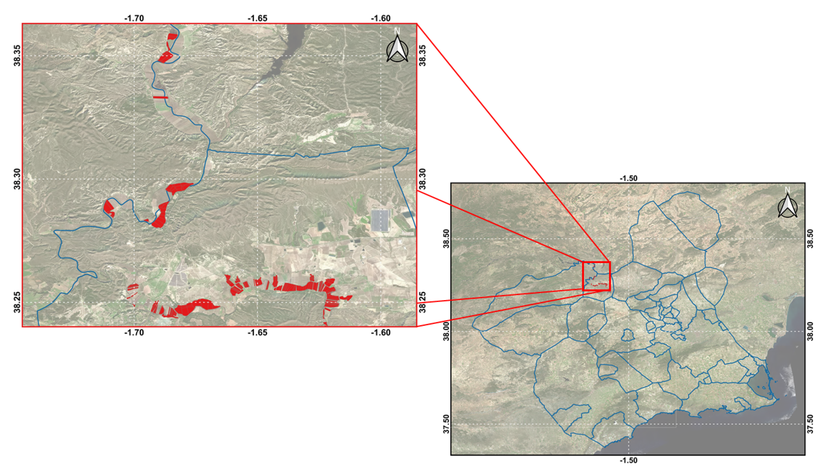
The area of interest for CbM—of the aid line associated with rice cultivation—is in the southeast of Spain, specifically in Calasparra (Coordinates: 38.13, −1.42) [30], which has an average elevation of between 300 and 500 m above sea level. It is a homogeneous rice planting area with an approximate extension of 10 km × 15 km, located in the northwest of Murcia, as shown in Figure 1.

The two main varieties of rice are Sendra and Bomba. They are under guarantee granted by the Regulatory Council of the Calasparra Designation of Origin (D.O. Calasparra) [31], regulated by the Royal Decree of 1 February 1908, which delimited the Coto Arrocero to three municipal boundaries: Hellín (Castilla La Mancha), Moratalla, and Calasparra. This rice reserve has an area of 2463 hectares.

The main characteristics of crop in the study area include that it is not grown in stagnant water but the water is extracted from the river to flood the plots. These plots are at different levels and are connected, causing a renewing current of water that maintains the correct water level at all times, returning the excess water to the river. Rice cultivation in this area has four phases: soil preparation, sowing, weeding, and harvesting.

For the 2019 campaign, there were 67 dossiers consisting of 306 declaration lines of support associated with rice, of which 301 belonged to declaration lines located in the Autonomous Community of the Region of Murcia, with a total of 336.76 hectares declared. Five declaration lines remained unmonitored, as they belonged to another Region.

Within the 2463 hectares of the “Coto Arrocero”, the monitored plots were located in three zones, as shown in Figure 1. Of the 301 declaration lines of aid associated with the rice crop to be monitored, 186 had less than one-hectare area and 109 less than 0.5 hectares. Seventy-one were between 1 and 2 hectares. Only six plots had an area of more than 5 hectares.

In the area, we can find an orography that causes the proliferation of small and heterogeneous plots, together with plantations of horticultural crops or legumes (an agricultural practice used to regenerate plots that have clayey soil). In any case, these circumstances complicate the identification of rice cultivation through biophysical indices.

3. Materials and Methods

3.1. Materials

The material proceed from two different data sources: RS data and Geographical Information System (GIS) data.

One of the functional elements of the Copernicus Integrated Ground Segment (IGS) is the Data and Information Access Services (DIAS) [32], which make Copernicus data and information available for access, and offer high processing capabilities in the cloud. To perform the processing tasks detailed in this work, in the DIAS environment called Creodias [33], a virtual machine was created under a Windows Server 2016 environment to carry out the related tasks, with eight processors (Intel Xeon Sandy Bridge), 32 GB RAM, and a 128 GB SSD hard disk, along with an additional 500 GB disk. The software used was PostgreSQL database with the PostGIS extension, QGIS, and Python 3.7 (Anaconda environment) using libraries such as scikit-learn, numpy, pandas, and gdal.

3.1.1. Remote Sensing Data

A time-series of 53 days are available between 1 January 2019 and 27 December 2019, with zero cloud coverage in the area, formed by the T30SXH tile and orbit number 051 found in the EPSG:32630 reference system [34]. The product type is S2MSI2A, whose main characteristics are processing level 2A, ortho-rectified and Universal Transverse Mercator (UTM) geocoded, BOA [35], and multi-spectral reflectance [36].

The bands from S2MSI2A product satellites used in this project have been B2, B3, B4 and B8 [37,38].

Table 1. S2 10 m bands.

Band	Spatial Resolution	Central Wavelength	Description
B2	10 m	490 nm	Blue
B3	10 m	560 nm	Green
B4	10 m	665 nm	Red
B8	10 m	842 nm	Near Infrared (NIR)

shows the technical information.

3.1.2. Geographic Information System Data

Vector information from the plots with support applications associated to rice for the 2019 campaign are available in the Aid Management System (SGA) application, developed by the Ministry of Agriculture of Spain through Fondo Español de Garantía Agrícola (FEGA). This application allows a user to export alphanumeric and graphical information in XML file format.

Each statement line is identified by the campaign file number, an application number, the applicant’s tax identification number, and a declaration line identifier regarding alphanumeric information. As regards geographical information, the applicant has the option of maintaining the definition of the parcel in the Geographical Information System of Agricultural Parcels (SIGPAC) [39] or manually redefining the parcel concerned.

3.2. Previous Analysis of the Coto Arrocero

In its technical guides, the JRC distinguishes three parts (or groups of activities) in the implementation of CbM:

• Preparation of monitoring in the years previous to its implementation (first phase);
• The year of initiation for the monitoring (second phase); and
• Horizontal activities not directly related to the processing of the application itself but the improvement of system efficiency (third phase).

The first section of the JRC’s technical guides deals with the identification of the uses and crops of the monitored zone in previous campaigns “Y-2”, “Y-1”, Y being the official starting campaign of CbM. Therefore, in our case, the 2017 and 2018 campaigns should be analyzed, as the first campaign for the monitoring controls was 2019.

The goal is to understand what useful information can be obtained from Sentinel data, based on the chosen area’s conditions for monitoring and the controlled regime. The processing of these data from previous campaigns must be completed, unrelated to the current campaign’s monitoring procedure.

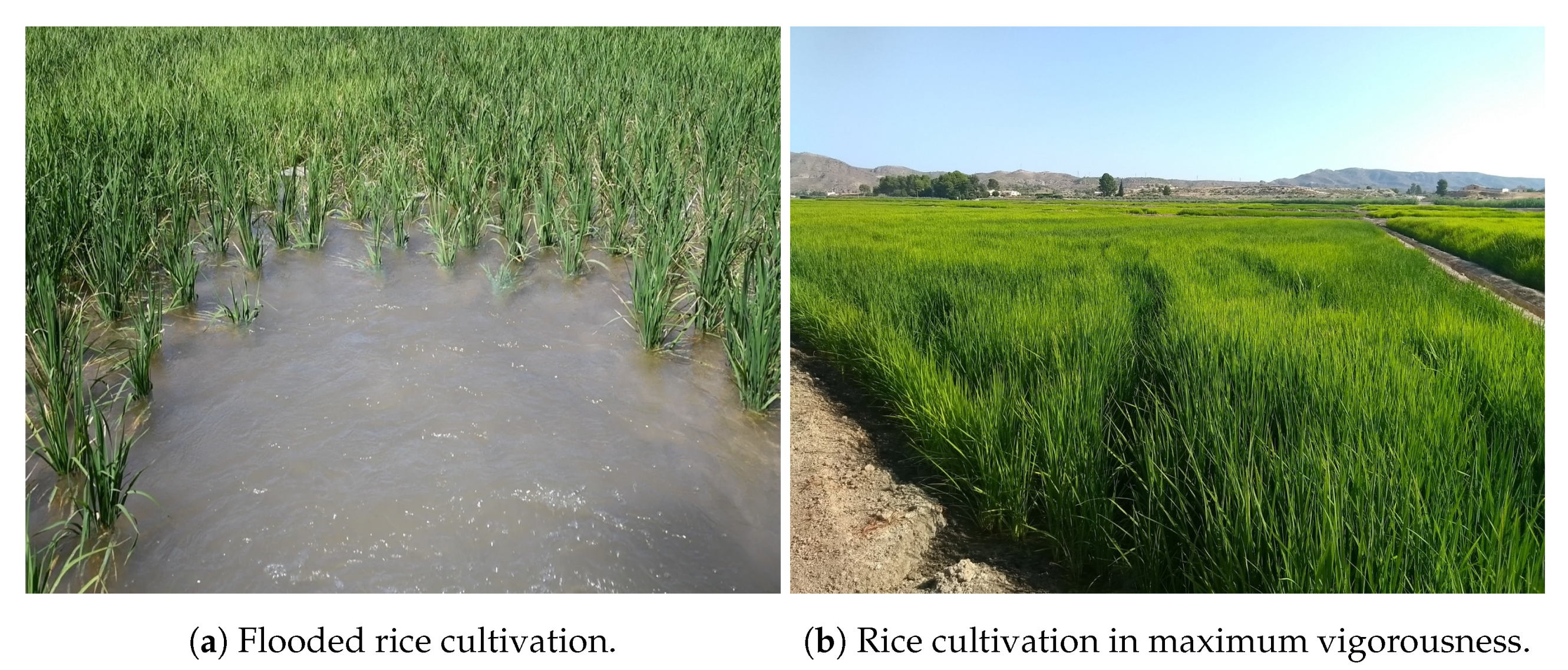
To fulfil the first phase, we opted to use a traditional RS approach. After consulting with the D.O. Calasparra regarding the characteristics of and the methods used for rice cultivation in the area, it was concluded that the main ones are the process of flooding the plots (Figure 2a) and the characteristic of vigour of the crop in the pre-harvest phase (Figure 2b). They also indicated that there may be a lag of four weeks in the implementation of agricultural practices and, therefore, in the crop’s evolution, depending on the plot’s location. Parcels are gravity irrigated with the Northern plots flooded first.

The indices that report the most information when obtaining the phenological curve [40,41,42] are the NDVI:

$$NDVI=\frac{B8-B4}{B8+B4},$$

(1)

and the Normalized Difference Water Index (NDWI):

$$NDWI=\frac{B3-B8}{B3+B8}.$$

(2)

Due to the need to automate the obtaining of the rice crop’s phenological curve using the NDVI and NDWI indices, an algorithm was implemented in Python to extract the zonal statistics of biophysical indices of the plots. The algorithm used S2 images of the time-series corresponding to 2017–2018. In brief, the implemented algorithm performed the following steps:

• Extraction of alphanumeric and geographic information from application declaration lines SGA and loading this information into the PostgreSQL database with PostGIS extension, in order to store all information generated by the implemented algorithms.
• Checking on the availability of S2 images (Bottom of Atmosphere, BOA) in the Creodias EO repository using the Finder tool [43] for a specific date and scene included in the area of study, as well as downloading S2 10 m bands through the Amazon Simple Storage Service [44]-based server, where the Creodias EO repository is accessible.
• Stacking of the four unloaded bands and clipping the generated raster [45] to fit the zone and, thus, speed up the process.
• Generation of level 3 products NDVI and NDWI [46] from the rasters generated in the previous step.
• Provision of several statistics (average, standard deviation, minimum, maximum, count, and sum) from the zonal statistics [47] between the parcel and the indices obtained in the previous step.
• Storage of calculated statistics for each of the parcels.
• The process is executed for each of the images obtained within the study campaign.

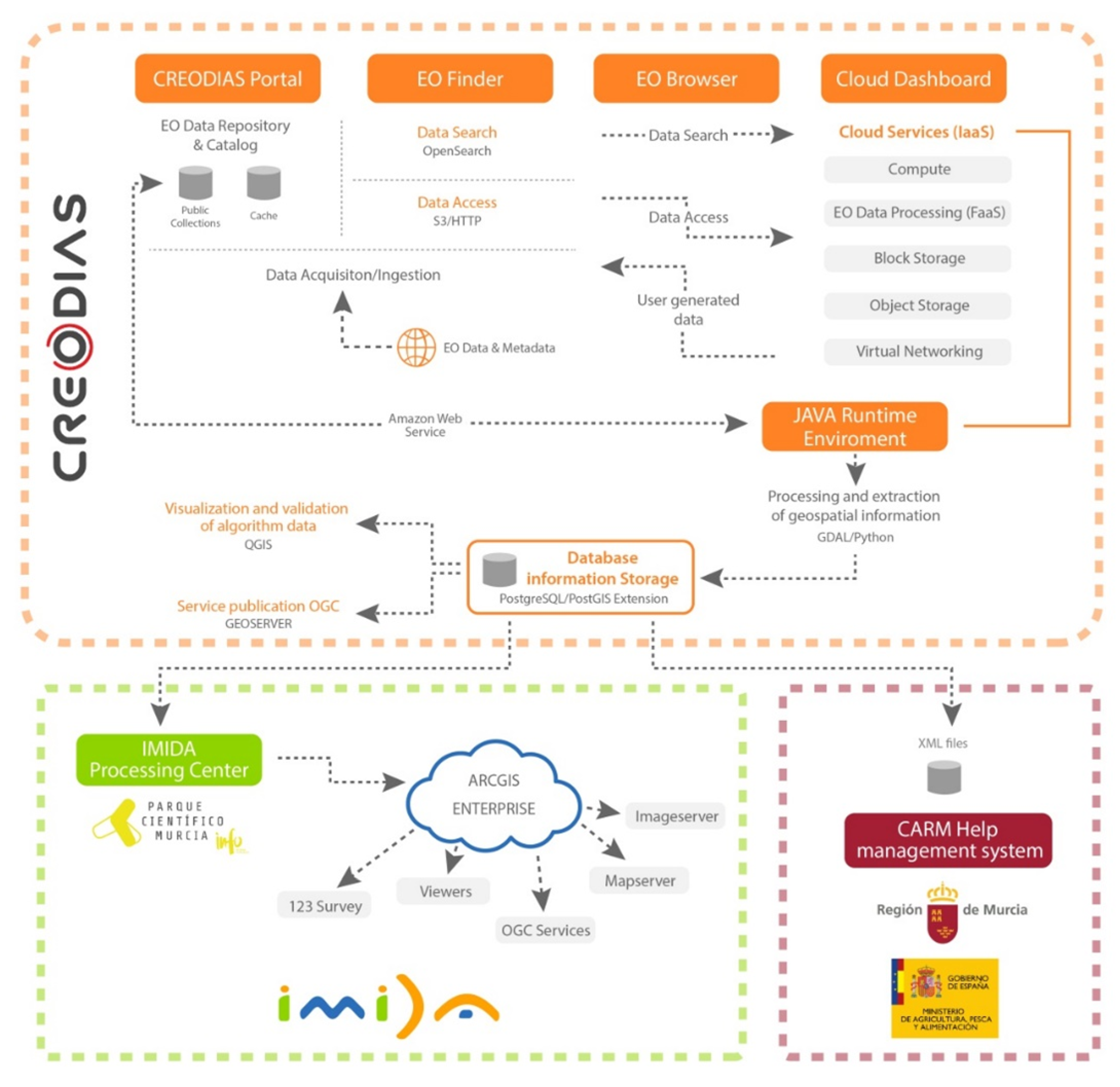
Figure 3 shows the infrastructure used to execute the analysis algorithm based on the methodology used in this work.

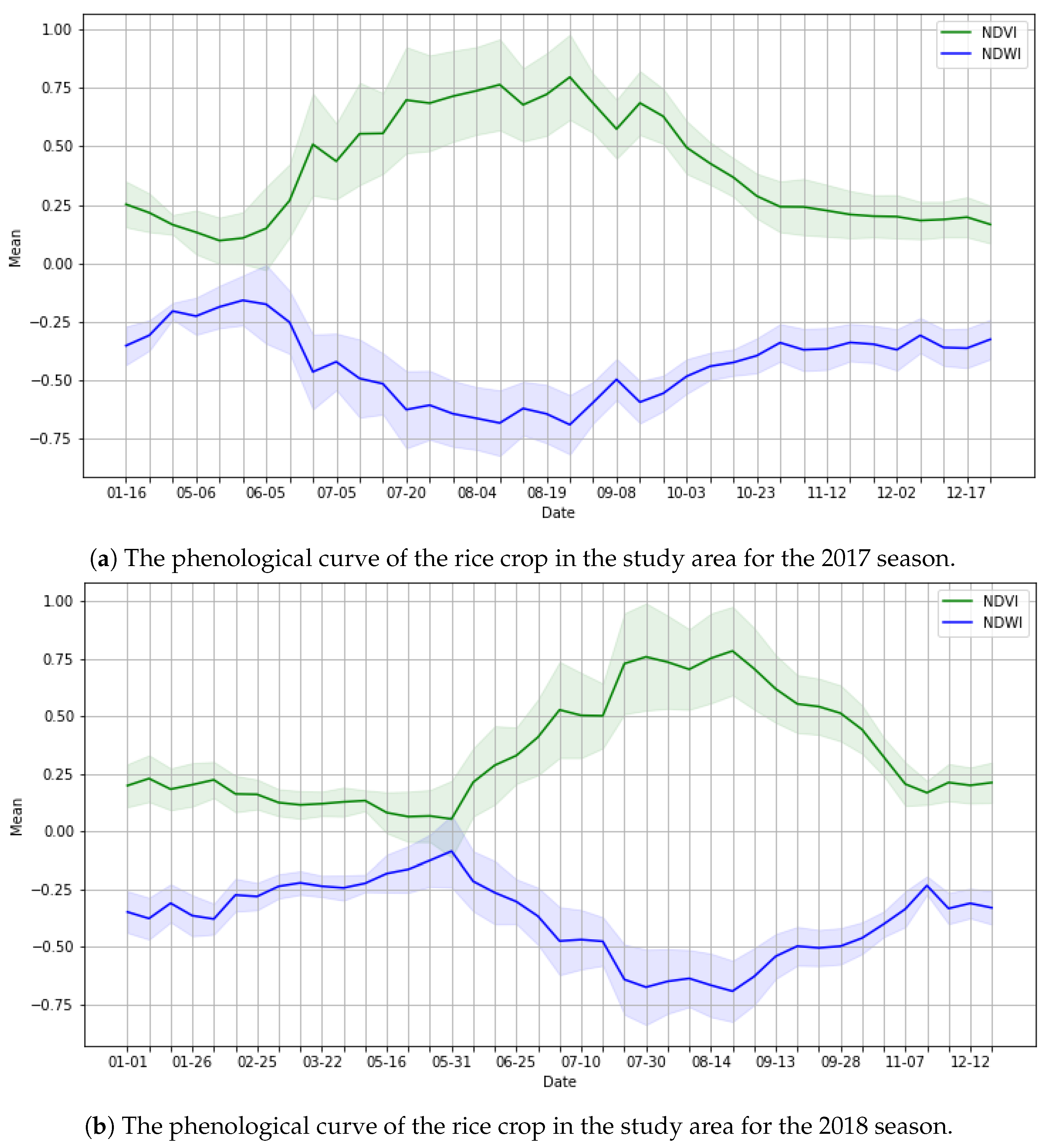
The phenological curves obtained for rice cultivation in the 2017 and 2018 campaigns are shown below, in Figure 4a,b, respectively. The time-series was composed of 38 dates for 2017 and 41 for 2018.

Analyzing the previous figures, we saw that there was a clear correlation between the NDVI and the NDWI [48], we could also determine the phases of rice cultivation, as shown in

Table 2. Rice cultivation phases in the Coto Arrocero area.

Phase	Start	End
Preparation	Early January	Early May
Flood	Early May	Mid June
Growth	Mid June	Early September
Collection	Early September	Mid October

.

Detailed analysis of the data indicated that a lag of about three weeks could occur between a given phase and its previous and subsequent phases.

Based on the conclusions obtained in phase 1 (Section 3.2), the NDVI and NDWI [49,50] rasters were incorporated into the process, along with the S2 bands (2, 3, 4, and 8). This information was used to compose the input variables of the learning matrix. Figure 5a,b show examples of the indices used on the dates for which they were most representative, which in the case of the NDWI is in early July and for the NDVI is in early September.

3.3. Methodology

3.3.1. Overview

Our objective was to implement an algorithm for crop identification [51]—specifically rice in the Coto Arrocero area—for CAP grant monitoring purposes through S2 data and ML. For this purpose, ML-based models were implemented using the Python scikit-learn [52,53] and XGBoost [54] libraries.

Figure 6 shows that, once the input information had been generated, the algorithm performed an initial assessment among many ML models [55,56], from which the most optimal one was chosen based on the information provided. Then, hyper-parameter optimization was performed for the selected model [57]. Once the classifier was ready, pixel-by-pixel prediction [58] was performed and, finally, validation of the used model was carried out [59].

The methodology used generates the most relevant data: a raster with the prediction made and a large volume of data (stored in the spatial database). The data available in the database are related to characteristics of the input data, classifier configuration, model evaluation and validation metrics, probabilities associated with each of the classes, and information on the zonal statistics between the plot and the generated raster.

This algorithm was executed as many times as images were available in the reference time-series; specifically, 53, as mentioned in the previous paragraph (Section 3.1). The main reason for this was the difference of four weeks in applying agricultural techniques on the plot, depending on where it was located, as discussed in Section 3.2; which we felt could cause some uncertainty in the model.

In principle, the implemented algorithm performed classification between two classes. However, it was defined with a high parameterization capability, in order to be used for the classification of more than two classes. Similarly, the input variables that will be part of the learning matrix and the necessary S2 scenes are configurable.

3.3.2. Data Preparation

So that ML models can do their work, the input information provided has to be array-like. Therefore, our vector and raster geographical information had to be transformed into a format understandable by these models.

The models used in the implemented algorithm were based on supervised learning. For this reason, the prediction was made based on the training data, which must be generated in a particular way, maintaining a balance between classes during classification and ensuring that they were sufficiently dispersed throughout the area of study.

The learning matrix (or ground-truth generation) was based on Regions of Interest (ROI) consisting of a series of polygons that indicated the areas rice in which was grown and those in which it was not. These ROIs were generated through a semi-automatic process implemented in Python and could belong to two classes:

• No Rice: value 1;
• Rice: value 80 (corresponds to the product code in the SGA application).

The class refers to the output variable; that is, what the ML model predicted.

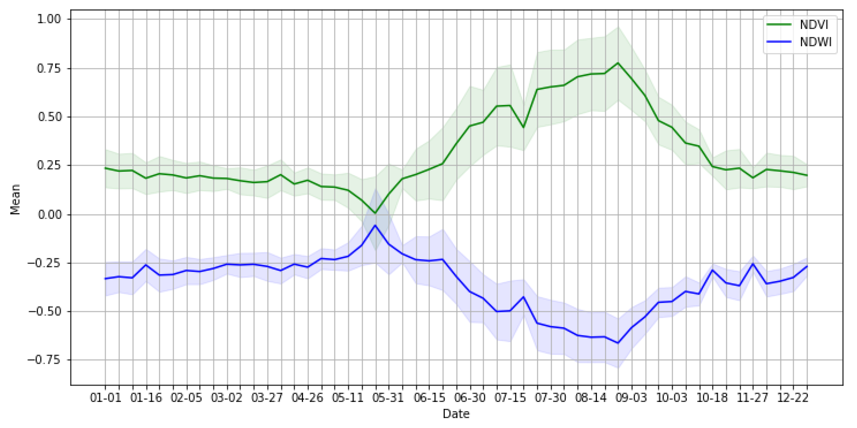
For the rice class, the mechanical part consisted of selecting the declaration line plots, which were fully adjusted (updated with the series treatments) to the phenological curve of the crop of the current campaign. Data from the current campaign’s phenological curve were obtained using the process reported in Section 3.2. The following formula was used to establish whether or not a plot was adjusted to the phenological curve represented in Figure 7:

$${\mu }_{NDVI}-2\sigma <={\mu }_i<={\mu }_{NDVI}+2\sigma ,$$

(3)

where ${\mu }_{NDVI}$ is the mean of the NDVI index for the current treatment date and $\sigma$ is the standard deviation.

The class corresponding to rice was formed from the parcels of the D.O. Calasparra, seeking to select those plots which grew rice in the current campaign and which have not requested aid for its cultivation, thus avoiding overfitting as much as possible. The objective here is to avoid as much as possible the inclusion in the learning matrix of those plots that will later have to be predicted. Thus avoiding that the model learns too well that learning matrix and favoring it can make predictions with high accuracy.

The class corresponding to the non-cultivation of rice was generated by digitizing polygon-type geometries manually on an S2 image, in areas where no rice was grown. The non-rice class mainly included elements that may have behavior and spectral response similar to rice cultivation, such as the horticultural and leguminous crops cited in Section 2 or, even, the wild vegetation proliferating in the mote of the river that crosses the Coto. In this case, approximately 20% was allocated to horticultural areas, 15% to legumes, 25% to wild vegetation in the riverbed, and the rest to other types of elements, such as areas of huge trees, scattered trees, tilled or bare soil, and so on.

A balanced data sample was obtained after generating the training matrix, with a fair percentage of rice and non-rice pixels sufficiently dispersed over the study area’s entire surface.

Once the learning matrix rows had been composed (as detailed in the previous step), we still had to define the column values obtained from the raster that included the S2 bands and the biophysical indices.

Following the lessons learned in phase 1, a raster was generated based on the S2 scene element of the corresponding time-series, consisting of bands 2, 3, 4, and 8 and the biophysical indices (NDVI and NDWI).

Finally, a raster with 1538 rows, 1003 columns, and six bands was available, with a total of 1,542,614 pixels.

Once the vector data had been generated from the ROIs and the raster onto which the values of those ROIs had been extracted, the values themselves were removed to form the array of input variables.

With regard to the transformation of the geometries into raster format so that values could be extracted from the tacked S2 image at the corresponding locations, the pixel distribution (among the classes to be classified) in the learning matrix is given in

Table 3. Learning matrix layout.

Class	Pixels	Percentage
No Rice (1)	2042	56.3
Rice (80)	1587	43.7

:

Finally, once the extracting values had been launched, the learning matrix was provided to the ML model to carry out the prediction.

To avoid random relationships between variables, it is good practice to subset data from the learning matrix into training data and test data [60]. As its name indicates, the training data set is used for fitting or model training, while the test data set is used to test the model and find the errors that occurred during the prediction. The test data set must never be used for training, and vice versa.

In this case, 75% of the learning samples were allocated for training and the remaining 25% for testing. In this process, randomness is also introduced in the input variables. Therefore, 2721 pixels remained for training and 908 for testing (498 of the non-rice class and 410 rice).

The learning matrix was composed of six input variables. Four of them (bands 2, 3, 4, and 8) contained values between 0 and 4.095. The remaining two (NDVI and NDWI), obtained from the previous ones, had values ranging from −1 to 1. The above results can lead to the predominance of one input variable over others when making predictions, making some more critical than others.

Table 4. Pairwise Pearson correlation coefficient for input variables.

	Band 2	Band 3	Band 4	Band 8	NDVI	NDWI
Band 2	1.00	0.98	0.97	0.74	−0.52	0.38
Band 3	0.98	1.00	0.97	0.78	−0.49	0.35
Band 4	0.97	0.97	1.00	0.76	−0.52	0.30
Band 8	0.74	0.78	0.76	1.00	0.060	−0.17
NDVI	−0.52	−0.49	−0.52	0.06	1.00	−0.91
NDWI	0.38	0.35	0.30	−0.17	−0.91	1.00

shows a table with Pearson’s correlation coefficient for the six input variables, observing the co-linearity between some variables:

Further, for many learning estimators, the standardization of the supplied data set is an indispensable requirement, as they may behave erratically if the individual characteristics do not resemble, more or less, the standard normal distribution.

To avoid the above, the algorithm performed standardization [61] of the input variables, consisting of a data rescale to have a mean ($\mu$) of zero and a standard deviation ($\sigma$) of one. This value was calculated as follows:

$$z=\frac{x-\mu }{\sigma }.$$

(4)

3.3.3. Model Evaluation

Once a learning matrix with properly separated and standardized data was available, we proceeded to evaluate a set of ML models [62] with the target of selecting the one that offered the best prediction capability.

The following types of estimators allow for classification [63]: Ensemble [64], Decision Trees, XGBoost [54], Neural Network, Naive Bayes, Neighbors, Linear, Discriminant, and Support Vector Machine.

The process made a pre-adjustment with training data and predicted the test data for each of the models. It should be clarified that in this phase, the models to be evaluated are defined without any adjustment, by which the hyper-parameters will have the pre-established default values. To perform a classification of the models, based on their performance, we used K-Fold Cross-Validation [65]. This method is an iterative process that consists of randomly dividing the data into k groups of approximately the same size. Then, k − 1 groups are used to train the model and one of the groups is used as a test set. This process is repeated k times, using a different group as the test set in each iteration. The process generates k test error estimates, whose average is used as the final estimate. In our case, the value of k was five.

K-Fold Cross-Validation was performed using the accuracy as a metric [66,67], as we had a balanced class distribution:

$$accuracy=\frac{true\_positives+true\_negatives}{total\_predictions}.$$

(5)

Thus, taking five different input data sets ensures that the accuracy obtained is adjusted and is reasonably reliable for evaluating each model’s performance.

3.3.4. Model Optimization

Once we had selected the estimator with which the classification was to be performed, its hyper-parameters were then optimized [68], in order to achieve classification as efficiently as possible, having the maximum possible score with the least overfit.

This part of the algorithm establishes a series of hyper-parameters and the range of values they could take and evaluates the classifier’s performance for each of the possible combinations for each type of classifier. Measures such as the score or the adjustment time are taken into account, in order to decide the best configuration. Furthermore, as described in Section 3.3.3, K-Fold Cross-Validation (k = 5) was used and the accuracy was used as a scoring metric.

For example, for ensemble classifiers, parameters such as the number of estimators (n_estimators), the function to measure the quality of the node divisions (criterion), the way to select the maximum number of elements for each tree (max_features), and the minimum number of elements to allow a new node split (min_sample_leaf) are optimized. In the case of XGBoost, parameters such as the number of estimators, learning rate, or maximum depth of a tree are optimized.

3.3.5. Classification

After the model has been optimized, the algorithm proceeded to adjust the model using the training data and S2 image prediction of our time-series. To predict class membership, the class probabilities were added together.

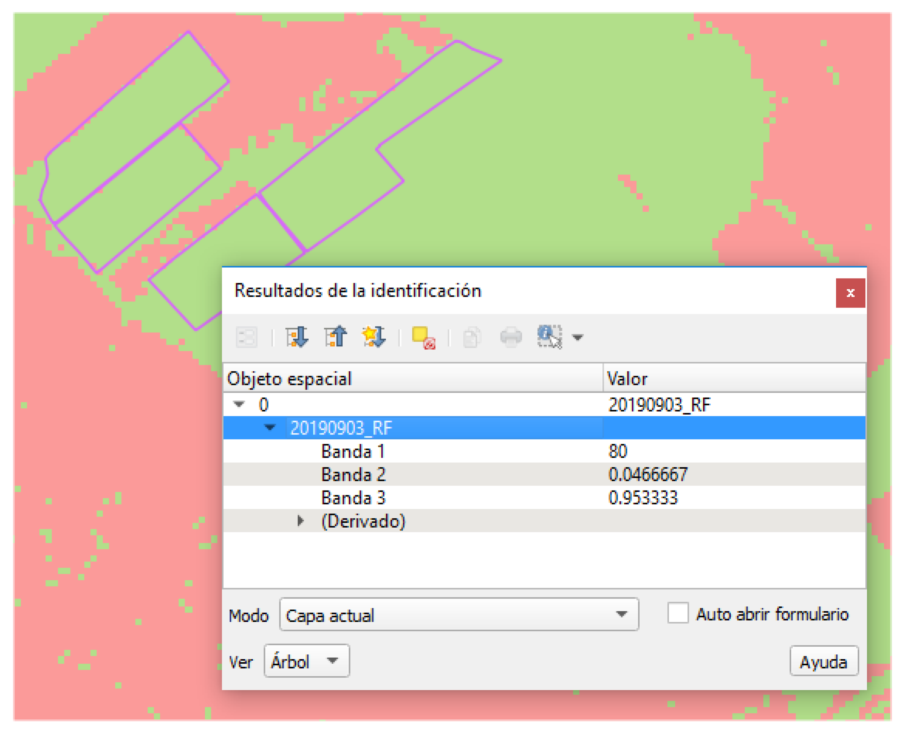
Based on the predicted output variable, together with the probability of belonging or not to the rice class, a raster was generated with the same characteristics of the used S2 image. For example, Figure 8 shows how the selected pixel was classified as rice (Band 1 = 80) with a probability of being rice of 95% (Band 3 = 0.953333) and a probability of not being rice of approximately 5% (Band 2 = 0.0466667). It should be clarified that this option only applies to those models that incorporate the functionality allowing association of probabilities to predictions. However, in this study, all the models selected finally presented this feature.

The first phase of the CbM is the so-called automatic and dealt with in this paper. In this automatic phase, the plots marked with yellow traffic light color will go to a phase called expert judgment. In this phase, an expert, based on information of all kinds, must indicate whether or not the plot is fulfilling the obligations of the aid requested. Therefore, products and functionalities such as those shown in Figure 8 can be very useful for the expert’s decision making.

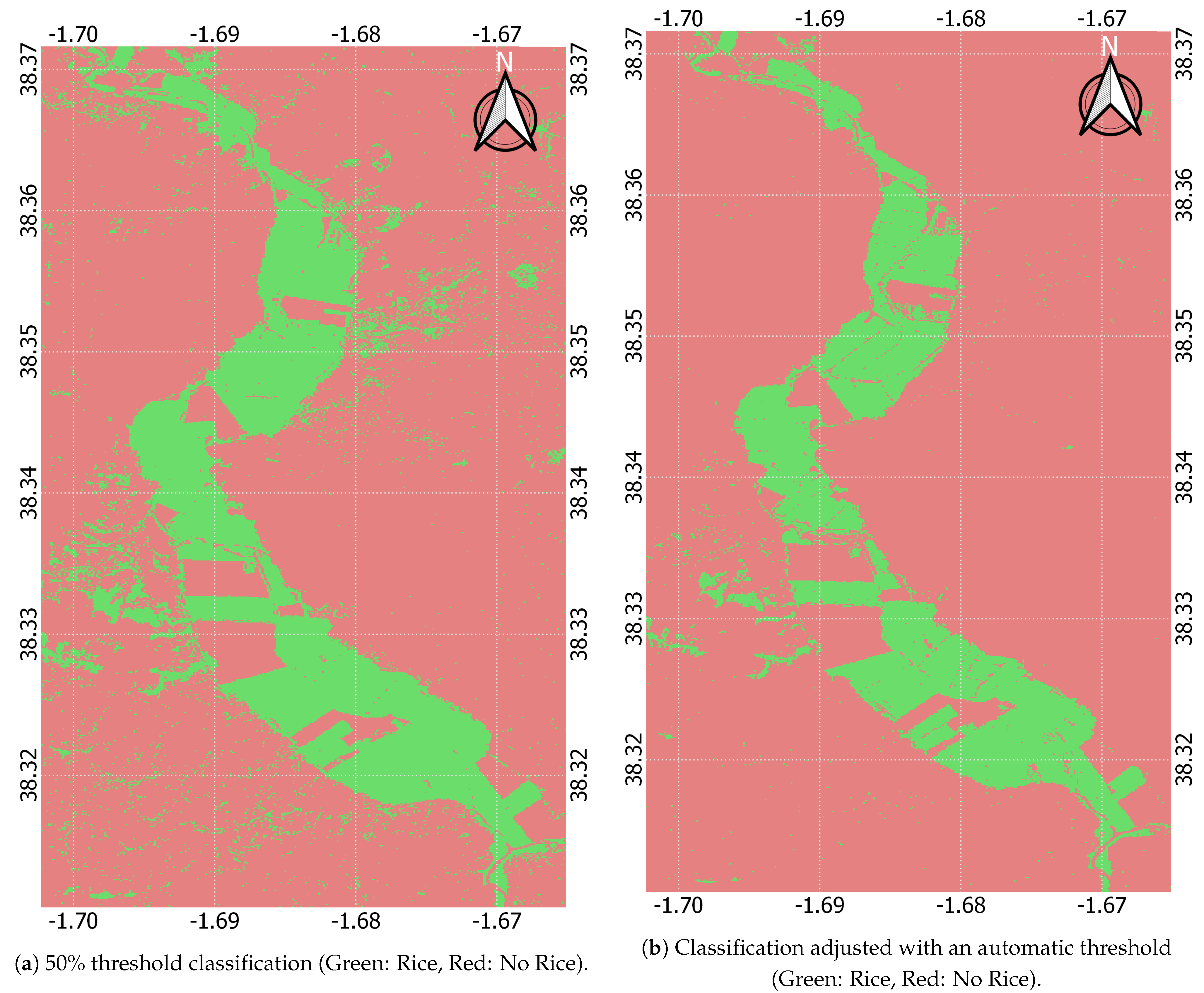
To avoid the maximum type 2 errors ($\beta$), false negatives, or false greens (Section 1), resulting in the payment of a non-corresponding grant, during classification, a process was implemented that allowed for adjustment of the threshold of probability that establishes membership of one class or another. By default, the estimators used 50% to establish this membership. The implemented algorithm allowed for obtaining an additional classification using a new membership threshold. If it is preferred to control this new threshold’s value, it can be set manually through the configuration file. If the parameter is not in the configuration file, the algorithm automatically sets it as the average probability of the pixels that were predicted as rice. Thus, this threshold may differ, depending on the time-series element.

$$x_i=80\leftrightarrow P\left(x_i\right)>=\mu \left(x_{class=80}\right).$$

(6)

Below is a comparison between the resulting raster with a threshold of 50% (Figure 9a) and the raster using the automatically established threshold (Figure 9b).

3.3.6. Validation

Once the original and adjusted predictions were available, the classifier was validated. For this purpose, data relating to different metrics [66,69] were recorded, including:

• Confusion Matrix: Not a metric, as such, but no less critical is a table-shaped visualization of the model’s predictions versus the ground-truth.
• Accuracy:

  $$accuracy=\frac{true\_positives+true\_negatives}{total\_predictions}.$$

  (7)
• Precision:

  $$precision=\frac{true\_positives}{true\_positives+false\_positives}.$$

  (8)
• Sensitivity or Exhaustivity (Recall or True Positive Rate, TPR):

  $$recall=\frac{true\_positives}{true\_positives+false\_negatives}.$$

  (9)
• F1 Score:

  $$f1\_score=\frac{2\ast precision\ast sensitivity}{precision+sensitivity}.$$

  (10)
• Specificity or False Positive Rate (FPR):

  $$specificity=\frac{true\_negatives}{true\_negatives+false\_positives}.$$

  (11)
• Kappa Score [70]:

  $$kappa=\frac{total\_accuracy-random\_accuracy}{1-random\_accuracy}.$$

  (12)
• Area under the curve (AUC): An aggregate measure of the performance of a binary classifier at all possible threshold values. It is the probability that the model ranks a random positive example higher than a random negative sample.

3.3.7. Zonal Statistics

Once the information derived from the validation of the corresponding estimator was recorded, it proceeded to obtain the zonal statistics [71] between the parcels and the raster generated during the prediction process. The purpose of the zonal statistic was to provide additional information to the classification, in order to facilitate crop identification; however, instead of being pixel-oriented, it is plot-oriented.

Among the statistics obtained were the typical mean, standard deviation, minimum, maximum, count, sum, and majority. At the zonal statistic level, the plots with the most pixels labeled rice were marked as rice crops and vice versa.

Furthermore, complementary statistics were added for each plot: number of pixels classified as rice, number of pixels classified as non-rice, the average probability of the plot being classified as rice or non-rice (based on the associated probabilities generated by the classifier for each of the pixels included in the plot), the reliability of the zonal statistics level classification (the fraction of the total number of pixels included in the plot that have been labeled as rice), as shown in the equation:

$$reliability\_zonal\_statistics=\frac{\sum pixel{s}_{class=80}}{|parcel\_pixels|},$$

(13)

and the average probability that the parcel was classified as rice or as non-rice; the latter based on the associated probabilities generated by the classifier for each of the pixels included in each of the plots.

Finally, the algorithm uses all the generated statistics to establish the traffic light color for each plot.

3.4. Validation of Results

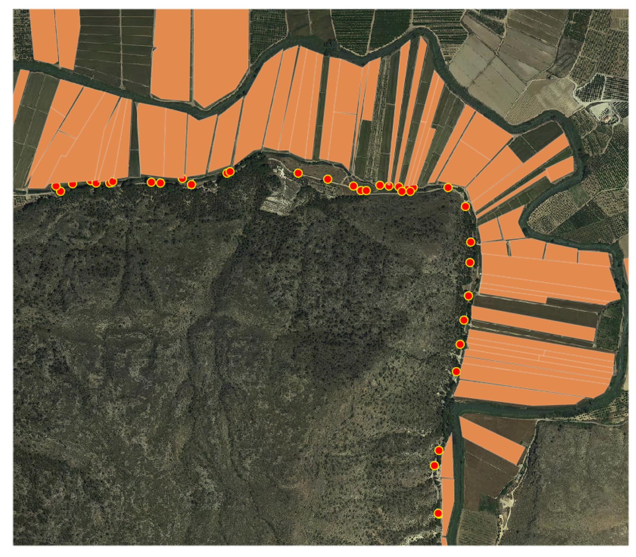
Two elements were used to validate the results offered by the algorithm manually. On one hand, ground-truth elements were used on a random set of plots generated by visits made at different times, taking photographs “in situ” and associating the geographical coordinates with each photographed plot, as shown in Figure 10. To improve the visualization of the plots under study, a process was carried out that extracts metadata from the photographs and stores them in a spatial database.

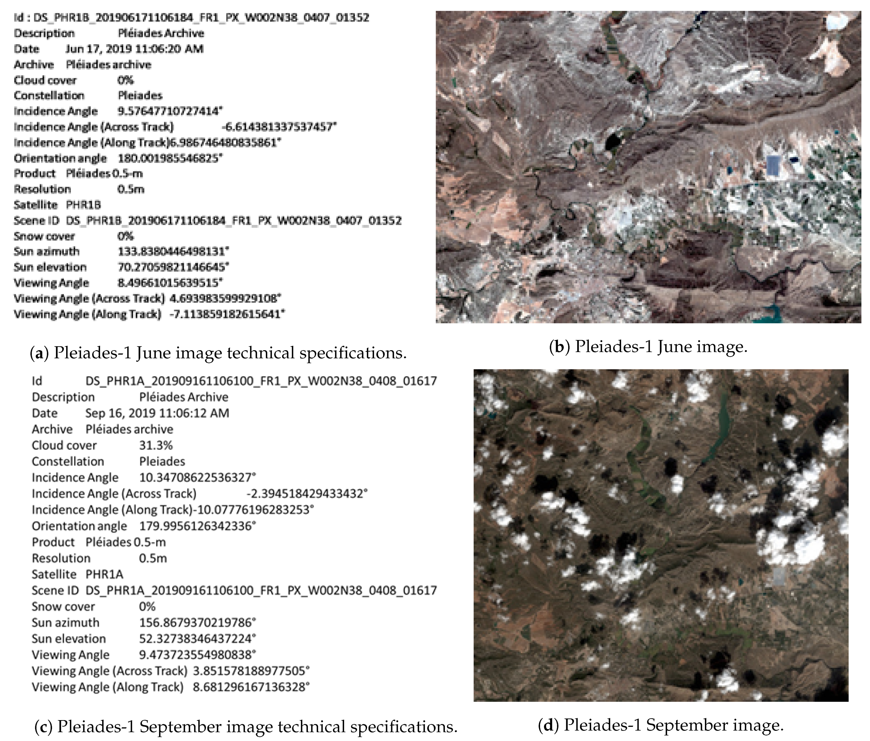
Moreover, as illustrated in Figure 11, HHR satellite images were used (specifically, Pleiades-1 [12]) with a spatial resolution of 50 cm. An image was requested by date to distinguish rice: in June, when the plots were flooded, and in September, the crop was at its maximum vigour.

In conjunction with the cited elements, the raster obtained from the classification, and using GIS tools (Figure 10), a visual validation was performed, which allowed us to assess the inconsistencies of the automatic and manual processes.

Furthermore, a quality assessment of CbM was carried out, following the indications of the technical guide issued by the JRC, which uses the same statistical assumptions of the binomial distribution underlying the international standard ISO document 2859/2 procedure B [72]. The control systems are based in the feedback of the data and methodology for that the result is less than that an error or be controlled, this is the reason why this phase is incorporated in all control systems [73].

4. Results

4.1. Use of Estimators

This section shows how the use of the different classifiers analyzed for the entire time series was distributed.

4.1.1. By Model Type

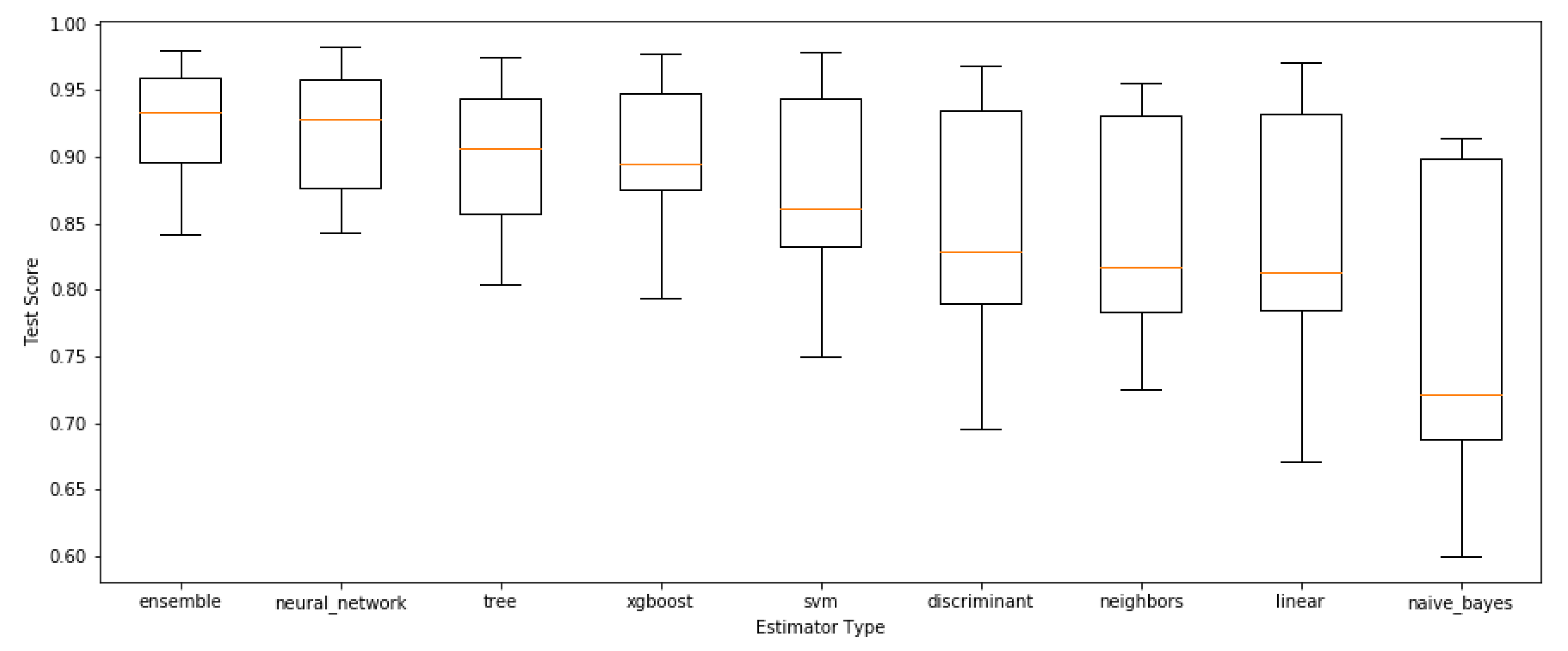
Figure 12 shows the accuracy obtained during the evaluation of the models, grouped by estimator type for the entire time-series analyzed. In this figure, the ends of the box represent the first (25th percentile) and third quartile (75th percentile), the line inside the box represents the median or second quartile (50th percentile). Finally, the end lines or whiskers show the range of the data. The overfitting observed is because the models in this phase are not fined tuned. This overfitting will disappear in the optimization phase of the selected model. It can be seen that the ensemble-type models were the ones that obtained the best scores:

Table 5. Use of estimators in classification grouped by type.

Type	Count	Percentage
ensemble	45	84.9
xgboost	5	9.4
neighbors	3	5.7

indicates that, for the 53 elements of the time-series, the type of estimator used the most times was the ensemble:

4.1.2. By Classifier

Table 6. Different metrics obtained by the classifiers for the entire time-series in the evaluation phase.

Classifier	Type	Accuracy	Precision	Recall	F1 Score
ExtraTrees	ensemble	0.93	0.94	0.94	0.94
RandomForest	ensemble	0.93	0.94	0.93	0.93
KNeighbors	neighbors	0.93	0.93	0.94	0.93
GradientBoosting	ensemble	0.92	0.93	0.93	0.93
XGBC	xgboost	0.92	0.93	0.93	0.93
MLP	neural network	0.91	0.92	0.93	0.92
DecisionTree	tree	0.90	0.91	0.92	0.91
SVC	svm	0.90	0.91	0.92	0.91
ExtraTree	tree	0.89	0.90	0.91	0.91
XGBCRandomForest	xgboost	0.87	0.89	0.89	0.89
QuadraticDiscriminant	discriminant	0.85	0.91	0.82	0.86
LogisticRegression	linear	0.84	0.85	0.87	0.86
GaussianNB	naive bayes	0.77	0.86	0.71	0.77

shows, using different metrics, the efficiency of each of the classifiers in the evaluation process for all of the dates of the time-series. A similar performance was observed among all the analyzed ensemble types, KNeighbors, and XGBC:

Table 7. Accuracy statistics obtained by the classifiers for the entire time-series in the evaluation phase.

Classifier	Min Accuracy	Mean Accuracy	Max Accuracy
ExtraTrees	0.80	0.93	0.98
RandomForest	0.79	0.93	0.98
KNeighbors	0.79	0.93	0.98
GradientBoosting	0.79	0.92	0.98
XGBC	0.79	0.92	0.98
MLP	0.77	0.91	0.98
DecisionTree	0.76	0.90	0.98
SVC	0.76	0.90	0.98
ExtraTree	0.74	0.89	0.98
XGBCRandomForest	0.68	0.87	0.98
QuadraticDiscriminant	0.68	0.85	0.97
LogisticRegression	0.60	0.84	0.97
GaussianNB	0.55	0.77	0.95

details the minimum, average, and maximum accuracies for each model obtained in the evaluation process. The minimum accuracy appeared when the rice crop was not noticeably present in the field, instead of the maximum precision. It can be seen that all the models analyzed had optimum performance when the crop was fully developed. When the crop was not present or was under development, some models had difficulties. The ensemble-type models, KNeighbors, and XGBC offered more balanced performance throughout the time-series.

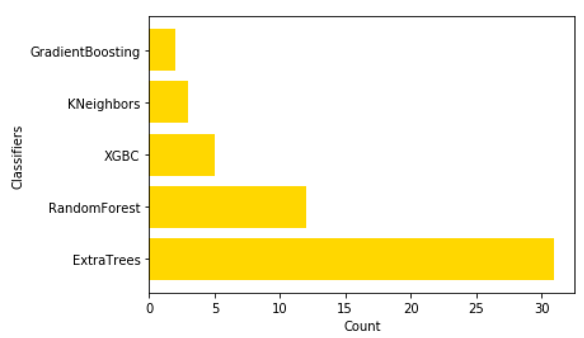
As a consequence of the information shown in Table 6 and Table 7, and as shown in Figure 13, it was concluded that the ExtraTrees classifier was the most-used in the 53 elements of the time-series. The RandomForest model also had some notoriety, although to a lesser extent. As can be seen, only five different models were used for classification in the whole time-series.

4.2. Model Optimization

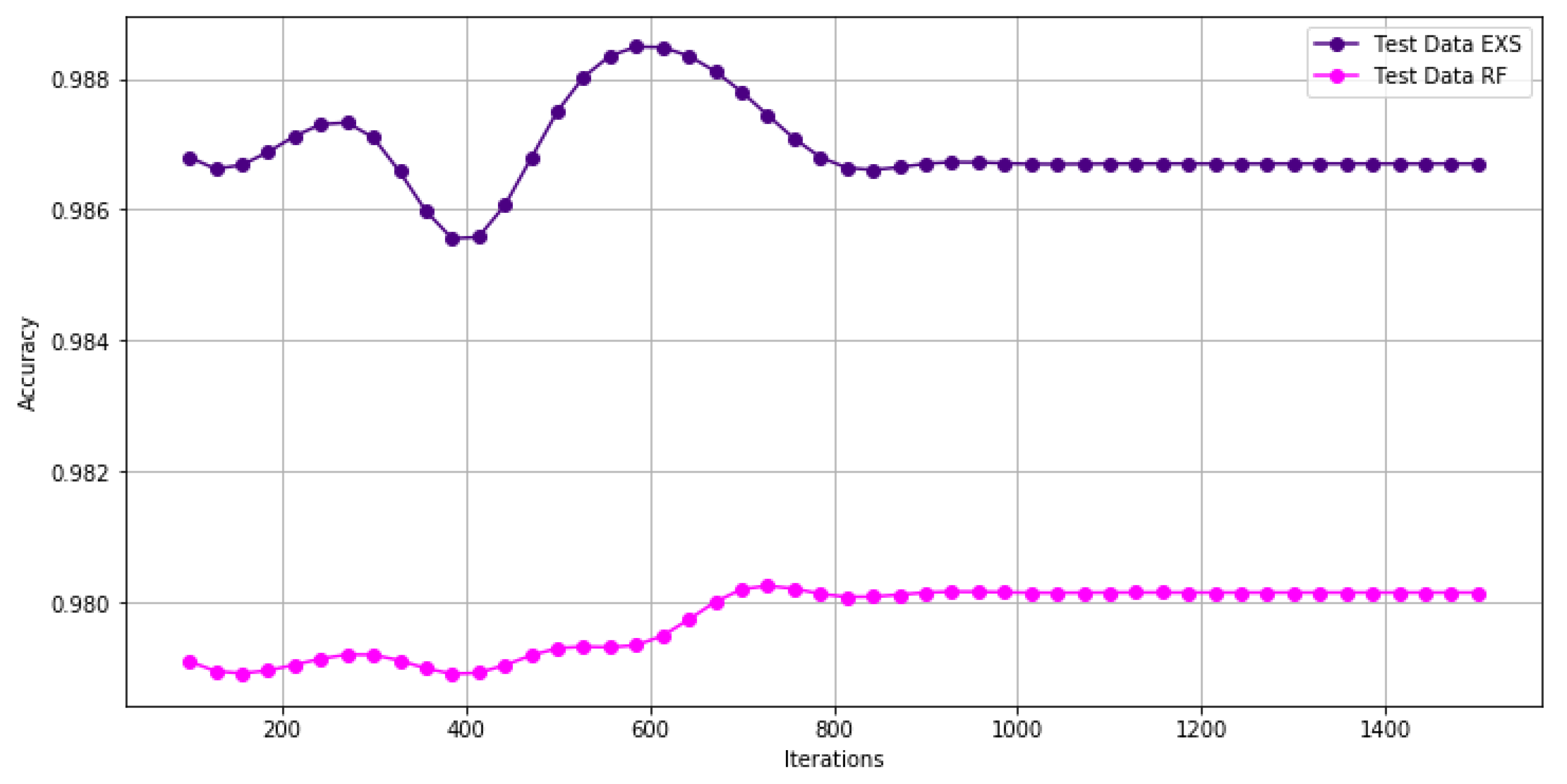
Figure 14 shows the validation curves of the two most-used models in the study—ExtraTrees and RandomForest. By analyzing these validation curves, it can be seen that, from 600–800 iterations, the model reached a plateau point, which gives us an idea that the classifier was correctly optimized, as the passage of further iterations does not increase the accuracy.

4.3. Input Variables Importance

Based on Figure 15, noting the average importance of each of the bands used, and taking into account the data provided by all the optimized models used during the classification of all the elements of the time-series, it can be concluded that there was no preponderance of one band over another, obtaining very similar percentages among the different input variables involved in the prediction of the output variables, thanks to the process of standardization.

4.4. Learning Matrix

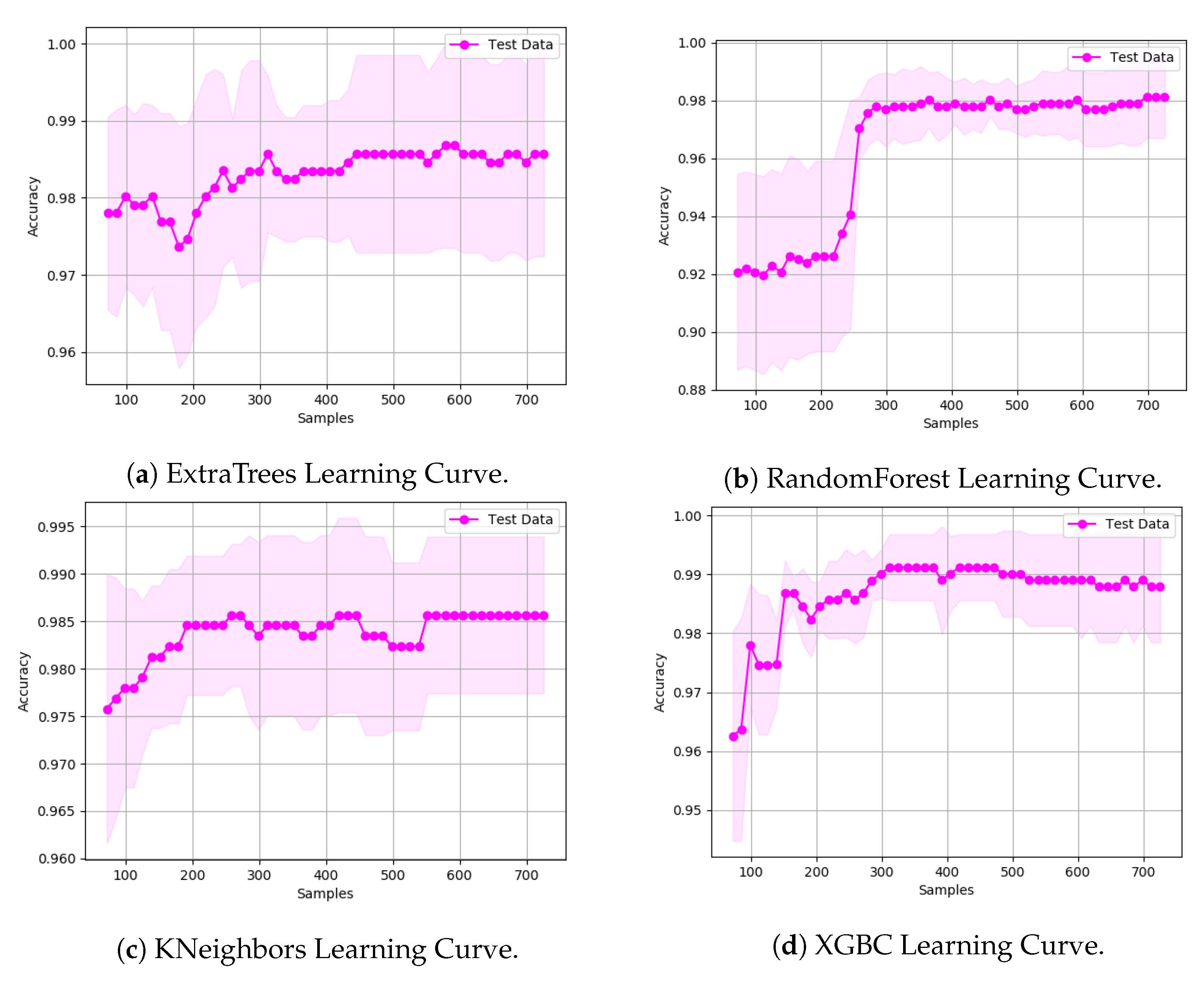
Looking at the learning curve generated during the model validation process, as shown in Figure 16, it can be observed that the accuracy reached a point of stability at around 500 samples; so, there will likely not be any significant improvement if we train with more data. In this study, the learning curve was used to measure the model performance and, so, the accuracy was used as a metric; in addition to being the metric used for the model evaluation and selection.

4.5. Model Validation

This section shows the results obtained in the validation phase through different elements.

4.5.1. Metrics

Analysis of the average scores of the metrics studied for the entire time-series, related to the rice crop and included in

Table 8. Average metric values analyzed for the entire time-series.

Metric	Score
Accuracy	0.934
Precision	0.942
Recall	0.940
F1 Score	0.941
Kappa	0.866
AUC	0.933
FPR	0.074

, provided very consistent and concordant results, indicating that the model did not demonstrate overfitting. These high values suggest that the model is capable of making useful predictions.

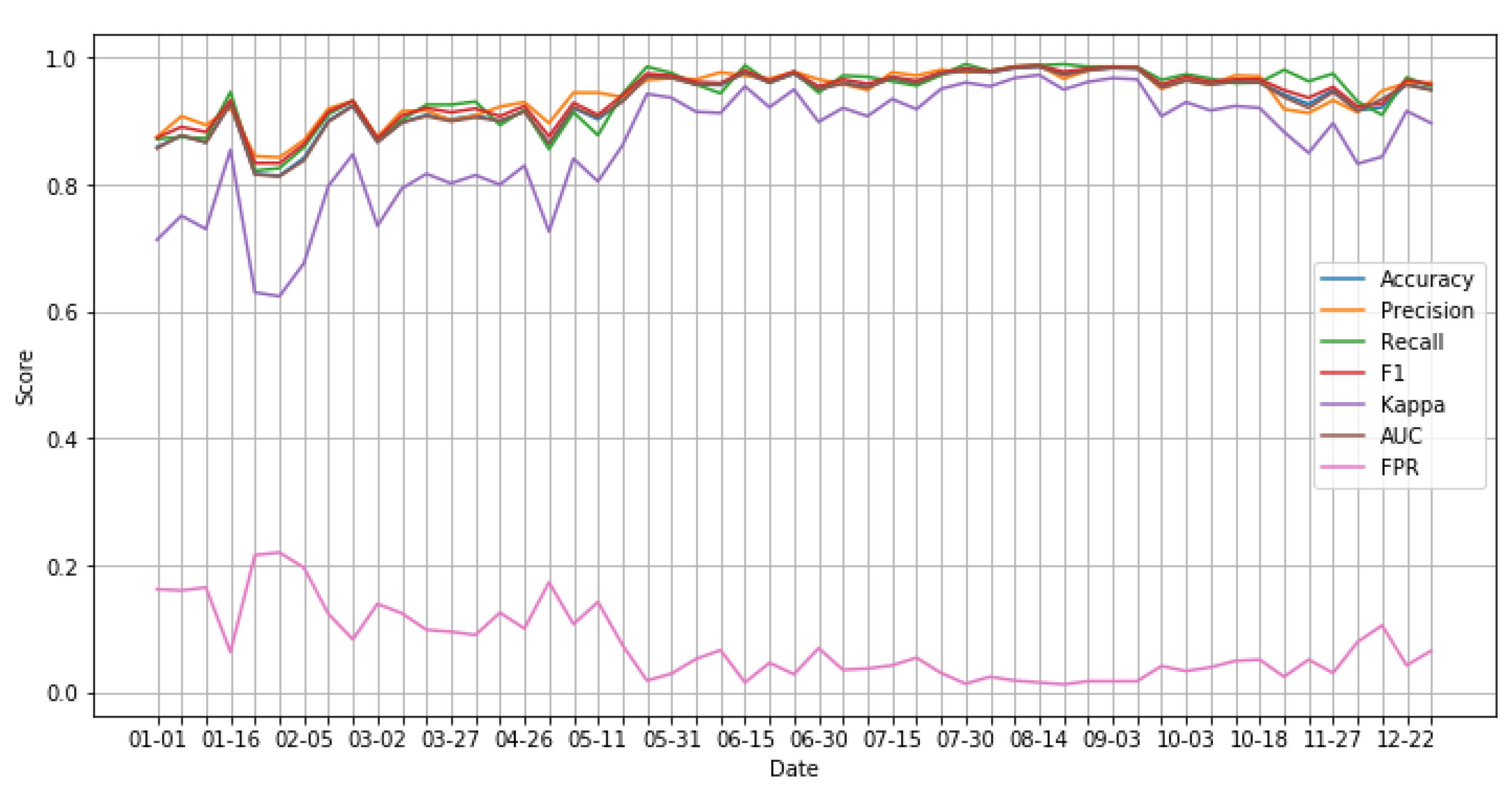
Figure 17 below shows the values of different metrics obtained by the models used in the analyzed time series. It can also be seen how higher scores were obtained for the dates at which the crop was developing; that is, from mid-May to the end of September.

Focusing only on the period in which the crop was easily identified by its peculiarities—between May and September—it can be observed that the scores associated with these metrics increased with some moderation, as shown in

Table 9. Average metric values analyzed between May and September.

Metric	Score
Accuracy	0.96
Precision	0.966
Recall	0.962
F1	0.964
Kappa	0.919
AUC	0.96
FPR	0.046

.

Comparison of Table 8 and Table 9 shows that it is not necessary to analyze the entire time series, but only to focus on the period between the flooding of the plots and the rice crop’s peak growth.

4.5.2. Confusion Matrix

Although the confusion matrix is not a metric itself, it can validate and check the designed model’s effectiveness. In this case, by analyzing the average values of the confusion matrix for the entire time-series results,

Table 10. Confusion matrix for the entire time series.

	No Rice	Rice	Sum
No Rice	449	51	500
Rice	61	347	408
Sum	510	395	908

was obtained.

Just as in the previous section, focusing on the months in which plot was flooded and the crop achieved its more significant vegetative development,

Table 11. Confusion matrix for time-series dates between May and September.

	No Rice	Rice	Sum
No Rice	470	28	498
Rice	38	372	410
Sum	508	400	908

shows how the confusion matrix values improved.

Comparison between Table 10 and Table 11 further indicates that it is not necessary to analyze the entire time-series.

4.6. Biophysical Indices vs. Machine Learning

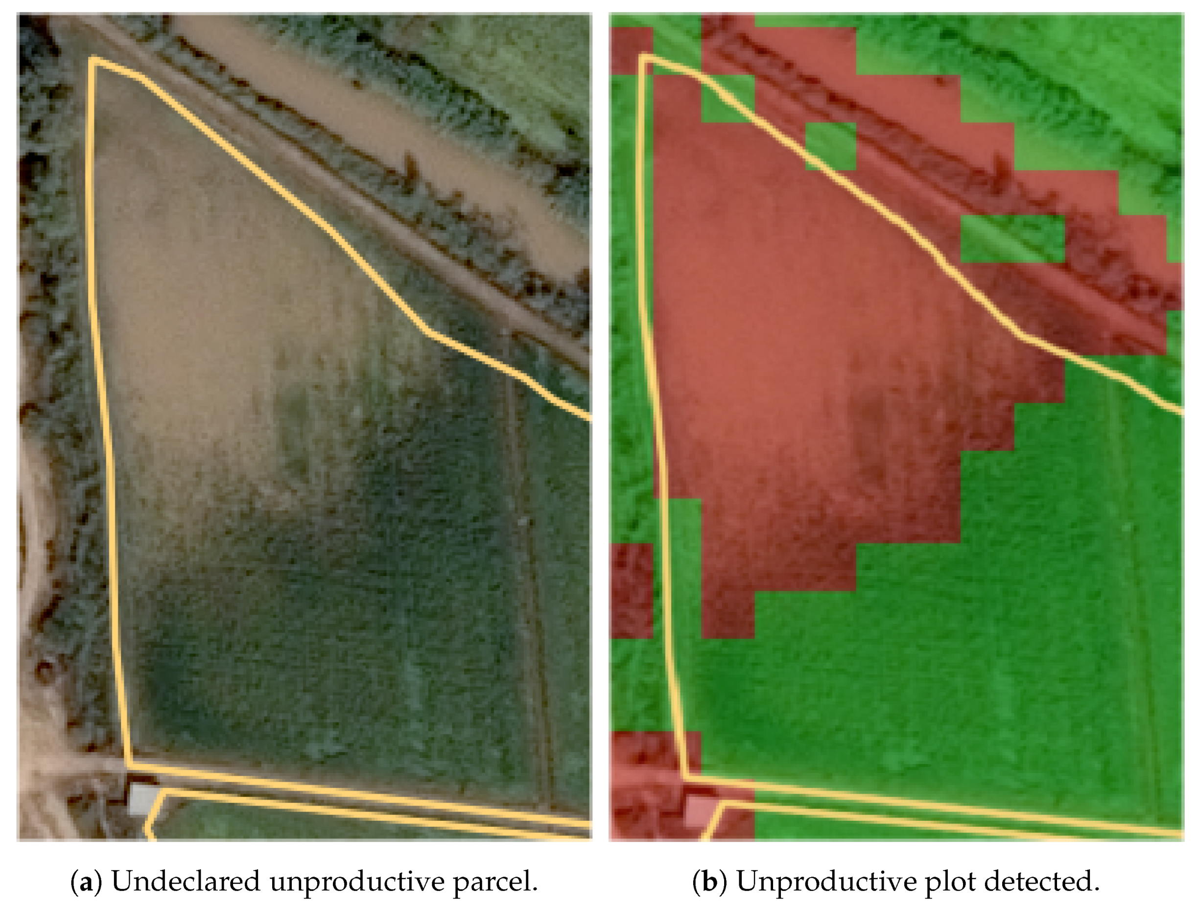
An approach to crop identification through RS could be the use of biophysical indices and, in any doubt, to proceed with classification using ML techniques. As an example, the plot associated with declaration line 227,743 in file 14,000,264 (Figure 18) clearly shows how aid had been requested for 100% of the total area of the parcel (black border) and, yet, only a part of this entire area had been cultivated:

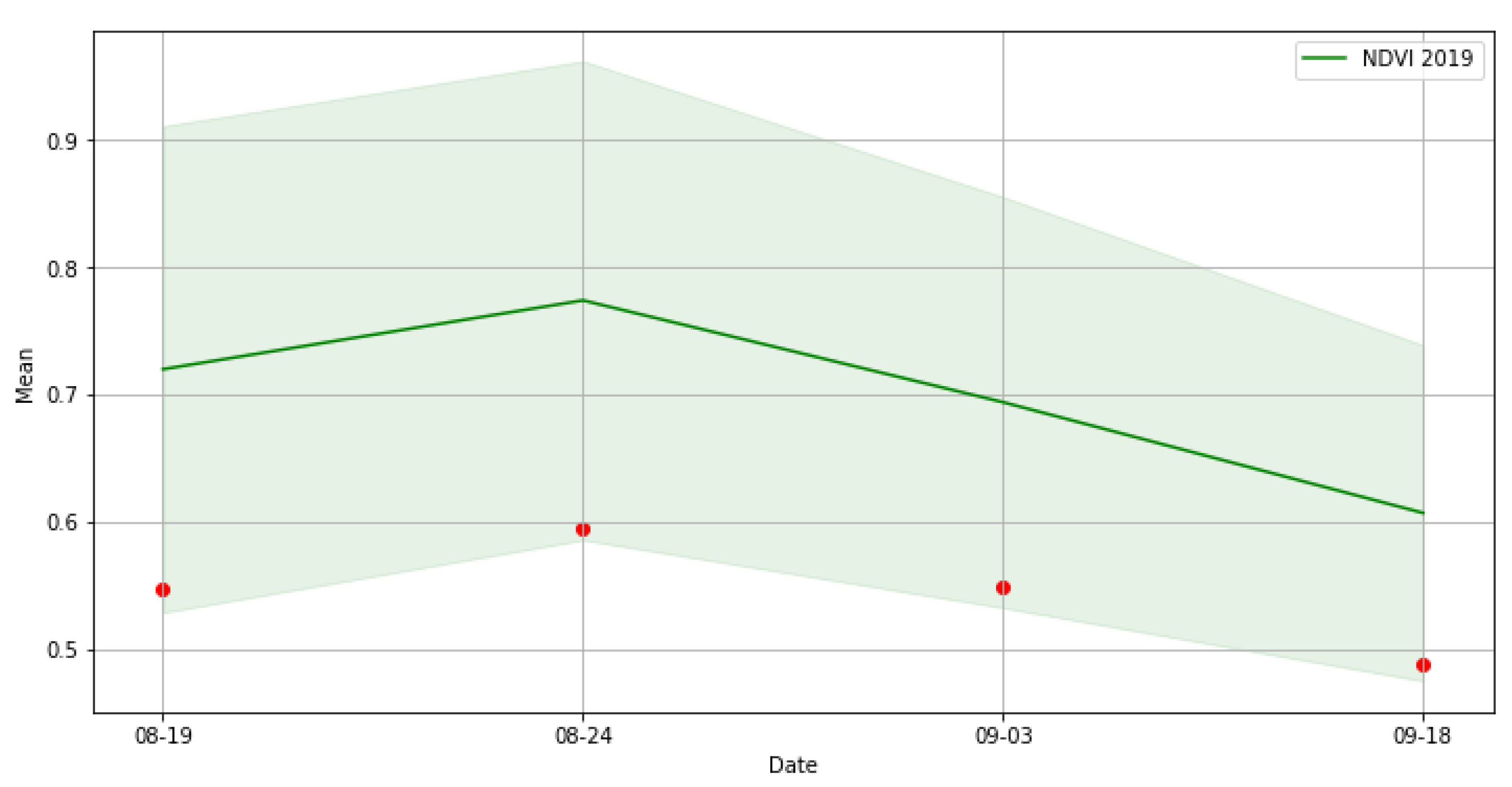
Once the parcel under study had been classified using NDVI (for crop vigour), it was classified with a green colour, indicating a type 2 error ($\beta$), as shown in Figure 19. Therefore, the parcel was considered, for all purposes, to comply with the conditions of the aid for the period from mid-August to mid-September, as shown in Figure 20. The NVDI was chosen as it considers the phenological curve obtained through the study’s processes in the two years before the 2019 campaign (Figure 7).

When using the parcel’s NDVI index mean values with a confidence interval of 2 times the standard deviation, pixels with vegetation predominate over those with no vegetation and cause the signal obtained to be within this confidence interval.

On the other hand, generating the classification through ML differentiates pixels in which there is a crop from those in which there is not, as shown in the following Figure 21.

Through the zonal statistics, referenced in Section 3.3.7, using the raster resulting from the classification, it was observed that half of the pixels of the plot were consistently marked as non-rice during the growth period of the rice crop, as shown in

Table 12. Pixel distribution of the zonal statistics for suspicious plot.

Date	Pixels Rice	Pixels Non-Rice
19 August 2019	48	51
24 August 2019	53	46
3 September 2019	47	52
18 September 2019	42	57

.

Even in less remarkable cases, as shown in Figure 22, the algorithm allows the user to set a threshold concerning the percentage of pixels marked as rice. Thus, if a plot exceeds this threshold, it will be assigned the green traffic light. In this way, it is possible to detect weak plots or parcels with cultivation problems.

Table 13. Percentage pixel distribution of the zonal statistics for weak plot.

Date	Percentage Pixels Rice	Percentage Pixels Non-Rice
19 August 2019	68	32
24 August 2019	64	36
3 September 2019	72	28
18 September 2019	74	26

shows the percentage of pixels detected as rice and non-rice for the example in Figure 22.

4.7. Results Validation

By applying the methodology for the validation of results described in Section 3.4, we found that the implemented algorithm could correctly predict not only all the cultivated rice plots but also those where it as not present and even those where it was partially present.

Out of the 301 monitored declaration lines, the algorithm predicted that 292 complied with the aid scheme’s obligations, and nine did not. After visual inspection of high-resolution satellite imagery and on-site visits in those cases where there were doubts, it was concluded that the algorithm was 100% correct in its predictions.

4.8. Reuse Calibrated Model

A preliminary analysis was carried out to check whether the calibrated model, generated as a result of the algorithm’s complete execution, could be used for campaigns in subsequent years.

Therefore, the 2019 campaign-calibrated model was used on a sample of dates of the 2020 campaign without cloud cover, and in which the crop was at its highest development point, obtaining the results of

Table 14. Test score for the test 2020 rice crop with the 2019 calibrated model.

Date	Test Score
29 July 2020	0.81
8 August 2020	0.86
13 August 2020	0.85
18 August 2020	0.85
28 August 2020	0.83

:

Although acceptable values were obtained, they were far from the 97% obtained for the same period of the 2019 campaign. Furthermore, if we consider that obtaining errors in the prediction can result in the payment of aid in cases where obligations are not met, we cannot use the calibrated model between different campaigns.

When, on the other hand, a new learning matrix was generated and the algorithm was launched from the beginning, the performance results of the 2020 campaign were similar to those of 2019.

In short, this preliminary analysis shows that a model calibrated for one campaign cannot be used for subsequent ones; however, the algorithm is valid for different campaigns.

5. Discussion

The objective of the study was to assess whether ML estimators can be valid for use in the CbM proposed by the EC, Regulation 2018/746 [4] of 18 May 2018, as a replacement for in-field checks; bearing in mind that controls must be carried out on 100% of aid declarations and continuously throughout the campaign. This regulation allows for the use of new technologies; above all, Sentinel data from the Copernicus Programme, particularly those of missions 1 and 2. As a sample, we decided to monitor rice cultivation in the area of Coto Arrocero of Calasparra (Murcia, Spain). We also contrasted methods based on biophysical indices with ML-based methods.

To achieve our goal, it was necessary to collect S2 data without cloud coverage; specifically, 53 days belonging to the 2019 campaign were chosen. After selecting the images, an algorithm was implemented to prepare data according to the needs of the ML classifiers. For validation of the data, a set of estimators was evaluated and, after choosing the best one, its hyperparameters were optimized to achieve the best possible prediction. The study area was then classified at pixel level (whether or not there was rice cultivation). Finally, the model was validated.

Analysis of the results showed that estimators used most often throughout the analyzed time-series were ensemble type and, within these, ExtraTrees performed best, followed by RandomForest. On the other hand, in terms of model efficiency, starting from 500 samples and 800 iterations, there was no gain in accuracy. In this environment, 93–94% accuracy, precision, sensitivity, and F1 score metrics were found for the entire time-series, which could be increased to 96% when considering time-series elements between May and September; that is, the months in which the crop’s vegetative development occurs. This increase clearly indicates that the full time-series does not need to be analyzed.

Additionally, the associated average probability of rice class membership for the entire time-series analyzed was 79% useful information for minimizing type 2 errors.

Furthermore, the model behaves particularly well in homogeneous short plots with a non-geometric structure. This capability can be used for error detection in aid statements or for the detection of unproductive areas in SIGPAC, due to the use of zonal statistics between the raster resulting from the prediction and the plot.

In the literature, different proposals are addressing the topic of rice crop detection using ML models. In the paper [74] they make use of the WEKA tool for the treatment of the input variables and the obtaining of results. At the same time, this work is finally transformed into a personalized tool in continuous improvement. Besides, this tool is used frequently and plays a key role in the allocation of CAP support. In the paper [75], data from several combined sensors is used to mapping rice crop. In this work, it has not been necessary to use other sensors such as the S1 SAR due to the low cloud cover in the study area. Besides, with the obtained metrics, especially during the period of greater representativeness of the cultivation, it is considered that the incorporation to the model of the data contributed by other sensors does not offer a remarkable improvement. Finally, paper [76] deals with the identification of rice cultivation through the use of recurrent neural networks (RNN) such as LSTM or Bi-LSTM, in addition to ML models. According to the most recent literature, RNNs are showing some improvement in crop identification compared to ML models.

Although this work is not exhaustive at the data split between training and testing level, as it could have been tested at both the pixel and the polygon level. In addition, model training tests could have been performed by eliminating the highly correlated variables. It would also be necessary to compare one classification with the dates treated individually vs. all dates treated together, or grouped by the different crop phases. Further analysis is also needed regarding the use of the calibrated model in subsequent campaigns. The methodology created in this work is the first approach to identify rice cultivation in this area through ML. The main idea is to improve it throughout subsequent agricultural campaigns by strengthening its weaknesses.

As for improvements in this line of research, besides treating the S2 dates available in a single data matrix instead of individual elements or grouped by the different phases of agricultural practice to use time as a predictor, we intend to adapt the methodology to the use of S1 images together with S2, and other input variables such as elevation or even agroclimatic data. The zonal statistics on the prediction raster will be further developed, in order to remove the information of pixels at plot boundaries and to ensure that the area declared for aid is the same as the area cultivated. Furthermore, we intend to incorporate a process that generates an image detecting the change produced in land-use and land-cover between two elements of the same time-series, through the use of methods based on biophysical indices and the ML PCA and KMeans models [77]. It is also intended to use RNNs to identify rice cultivation in the area and to be able to compare the results offered, with those obtained in this work. Finally, we will use the developed methodology to try to identify other crops located in disparate areas, thus taking advantage of the main features of the implemented algorithm, including its general purpose, scalability, and automation options.

6. Conclusions

The implement a methodology for crop identification according to the CAP grant monitoring purposes using S2 data and ML was achieved as well as the objective of our research. It defined a methodology which is capable of identifying rice cultivation in the area of Coto Arrocero in the Region of Murcia through ML, using S2 data (bands 2, 3, 4, and 8) and the NDVI and NDWI biophysical indices, without any one of them prevailing over the others. The average of the analyzed metrics for the whole time-series was around 93% and standard deviation of 1%. Supposing we focus only on the period of the full development of the crop—between May and September—the result obtained could be increased to 96% (±1%), which indicates that it is unnecessary to analyze the entire time-series, implying corresponding resource savings. It was also concluded that the most appropriate type of model for the identification of this crop was the so-called ensemble and, more specifically, the Extra-Trees and Random Forest models. These classifiers were very consistent in predicting the entire time-series and provided correct results when the crop was not yet at the peak of development.

The methodology created in this work can serve as a tool used periodically to establish those farmers which comply with the aid conditions and return the amount of assistance received. This solution’s definition entails a great change of culture and awareness in Public Administrations, promoting digital services that allow: increasing productivity and efficiency in their internal operation, implementing intelligent corporate management of data, and reducing time in administrative procedures.

In conclusion, this study’s results indicate that the CbM proposed by the EC for CAP aids, specifically those associated with rice cultivation, can be carried out through ML ensemble-type models with a reasonably high level of precision. The main novelty of this work is implementing a tool that helps the Administrations promote their digital transformation to manage the aids granted by the CAP, and that will be mandatory between the years 2021 and 2022. Besides, we must take into account not only the area of study, which has never been investigated by RS but the particular characteristics of its production system, less intensive than in other areas, so that the spectral signatures of rice are less defined, which implies difficulties not usually found in other areas of cultivation.

An innovative element of the proposed system is that all the results generated by the methodology are integrated into the Administration’s file management platform, allowing a greater resolution of files and the detection of 7% more files that did not comply with the obligations to receive the aid. Further, it was discovered that the defined methodology could also be used to detect heterogeneous parcels and whether they are unproductive or abandoned areas. As proposed, it can be used as a substitute for on-site inspections; over 5% of the dossiers in a specific moment can be checked through RS, or over 100% of the dossiers during the whole season.

References

1. CAP Summary. Available online: https://ec.europa.eu/info/food-farming-fisheries/key-policies/common-agricultural-policy/cap-glance_en (accessed on 2 April 2020).
2. Van Zanten, B.T.; Verburg, P.H.; Espinosa, M.; Gomez-y Paloma, S.; Galimberti, G.; Kantelhardt, J.; Kapfer, M.; Lefebvre, M.; Manrique, R.; Piorr, A.; et al. European agricultural landscapes, common agricultural policy and ecosystem services: A review. Agron. Sustain. Dev. 2014, 34, 309–325. [Google Scholar] [CrossRef] [Green Version]
3. Regulation 1306/2013. Available online: https://eur-lex.europa.eu/legal-content/EN/TXT/PDF/?uri=CELEX:32013R1306&from=en (accessed on 21 October 2020).
4. Regulation 2018/746. Available online: https://eur-lex.europa.eu/legal-content/EN/TXT/PDF/?uri=CELEX:32018R0746&from=EN (accessed on 2 April 2020).
5. European Space Agency. Available online: https://www.esa.int (accessed on 4 April 2020).
6. Sentinel Missions. Available online: https://sentinel.esa.int/web/sentinel/home (accessed on 3 April 2020).
7. Zhao, Y.; Potgieter, A.B.; Zhang, M.; Wu, B.; Hammer, G.L. Predicting wheat yield at the field scale by combining high-resolution Sentinel-2 satellite imagery and crop modelling. Remote Sens. 2020, 12, 1024. [Google Scholar] [CrossRef] [Green Version]
8. Buma, W.G.; Lee, S.I. Evaluation of Sentinel-2 and Landsat 8 Images for Estimating Chlorophyll-a Concentrations in Lake Chad, Africa. Remote Sens. 2020, 12, 2437. [Google Scholar] [CrossRef]
9. Bazzi, H.; Baghdadi, N.; El Hajj, M.; Zribi, M.; Minh, D.H.T.; Ndikumana, E.; Courault, D.; Belhouchette, H. Mapping paddy rice using Sentinel-1 SAR time series in Camargue, France. Remote Sens. 2019, 11, 887. [Google Scholar] [CrossRef] [Green Version]
10. Sitokonstantinou, V.; Papoutsis, I.; Kontoes, C.; Lafarga Arnal, A.; Armesto Andrés, A.P.; Garraza Zurbano, J.A. Scalable parcel-based crop identification scheme using sentinel-2 data time-series for the monitoring of the common agricultural policy. Remote Sens. 2018, 10, 911. [Google Scholar] [CrossRef] [Green Version]
11. Joint Research Centre. Available online: https://ec.europa.eu/jrc/en (accessed on 4 April 2020).
12. Maxwell, A.E.; Warner, T.A.; Fang, F. Implementation of machine-learning classification in remote sensing: An applied review. Int. J. Remote Sens. 2018, 39, 2784–2817. [Google Scholar] [CrossRef] [Green Version]
13. Paredes-Gómez, V.; Gutiérrez, A.; Del Blanco, V.; Nafría, D.A. A Methodological Approach for Irrigation Detection in the Frame of Common Agricultural Policy Checks by Monitoring. Agronomy 2020, 10, 867. [Google Scholar] [CrossRef]
14. Campos-Taberner, M.; García-Haro, F.J.; Martínez, B.; Sánchez-Ruíz, S.; Gilabert, M.A. A copernicus sentinel-1 and sentinel-2 classification framework for the 2020+ European common agricultural policy: A case study in València (Spain). Agronomy 2019, 9, 556. [Google Scholar] [CrossRef] [Green Version]
15. Campos-Taberner, M.; García-Haro, F.J.; Busetto, L.; Ranghetti, L.; Martínez, B.; Gilabert, M.A.; Camps-Valls, G.; Camacho, F.; Boschetti, M. A critical comparison of remote sensing leaf area index estimates over rice-cultivated areas: From Sentinel-2 and Landsat-7/8 to MODIS, GEOV1 and EUMETSAT Polar system. Remote Sens. 2018, 10, 763. [Google Scholar] [CrossRef] [Green Version]
16. ERMES—An Earth Observation Model Based Rice Information Service. Available online: http://www.ermes-fp7space.eu/es/homepage/ (accessed on 10 February 2021).
17. Final Report Summary-ERMES (ERMES: An Earth obseRvation Model based RicE information Service). Available online: hhttps://cordis.europa.eu/docs/results/606/606983/final1-ermes-final-report-v2-1a2.pdf (accessed on 10 February 2021).
18. Son, N.T.; Chen, C.F.; Chen, C.R.; Guo, H.Y. Classification of multitemporal Sentinel-2 data for field-level monitoring of rice cropping practices in Taiwan. Adv. Space Res. 2020, 65, 1910–1921. [Google Scholar] [CrossRef]
19. Cai, Y.; Lin, H.; Zhang, M. Mapping paddy rice by the object-based random forest method using time series Sentinel-1/Sentinel-2 data. Adv. Space Res. 2019, 64, 2233–2244. [Google Scholar] [CrossRef]
20. Ali, A.M.; Savin, I.; Poddubskiy, A.; Abouelghar, M.; Saleh, N.; Abutaleb, K.; El-Shirbeny, M.; Dokukin, P. Integrated method for rice cultivation monitoring using Sentinel-2 data and Leaf Area Index. Egypt. J. Remote Sens. Space Sci. 2020. [Google Scholar] [CrossRef]
21. Tucker, C. Red and Photographic Infrared Linear Combinations for Monitoring Vegetation. Remote Sens. Environ. 1979, 8. [Google Scholar] [CrossRef] [Green Version]
22. D’Odorico, P.; Gonsamo, A.; Damm, A.; Schaepman, M.E. Experimental evaluation of Sentinel-2 spectral response functions for NDVI time-series continuity. IEEE Trans. Geosci. Remote Sens. 2013, 51, 1336–1348. [Google Scholar] [CrossRef]
23. Falanga Bolognesi, S.; Pasolli, E.; Belfiore, O.R.; De Michele, C.; D’Urso, G. Harmonized Landsat 8 and Sentinel-2 Time Series Data to Detect Irrigated Areas: An Application in Southern Italy. Remote Sens. 2020, 12, 1275. [Google Scholar] [CrossRef] [Green Version]
24. Madigan, E.; Guo, Y.; Pickering, M.; Held, A.; Jia, X. Quantitative Monitoring of Complete Rice Growing Seasons Using Sentinel 2 Time Series Images. In Proceedings of the IGARSS 2018—2018 IEEE International Geoscience and Remote Sensing Symposium, Valencia, Spain, 22–27 July 2018; pp. 7699–7702. [Google Scholar] [CrossRef]
25. Nelson, A.; Setiyono, T.; Rala, A.B.; Quicho, E.D.; Raviz, J.V.; Abonete, P.J.; Maunahan, A.A.; Garcia, C.A.; Bhatti, H.Z.M.; Villano, L.S.; et al. Towards an operational SAR-based rice monitoring system in Asia: Examples from 13 demonstration sites across Asia in the RIICE project. Remote Sens. 2014, 6, 10773–10812. [Google Scholar] [CrossRef] [Green Version]
26. Setiyono, T.; Holecz, F.; Khan, N.; Barbieri, M.; Quicho, E.; Collivignarelli, F.; Maunahan, A.; Gatti, L.; Romuga, G. Synthetic Aperture Radar (SAR)-based paddy rice monitoring system: Development and application in key rice producing areas in Tropical Asia. IOP Conf. Ser. Earth Environ. Sci. 2017, 54, 012015. [Google Scholar] [CrossRef] [Green Version]
27. Uto, K.; Seki, H.; Saito, G.; Kosugi, Y. Characterization of rice paddies by a UAV-mounted miniature hyperspectral sensor system. IEEE J. Sel. Top. Appl. Earth Obs. Remote Sens. 2013, 6, 851–860. [Google Scholar] [CrossRef]
28. Hashimoto, N.; Saito, Y.; Maki, M.; Homma, K. Simulation of reflectance and vegetation indices for unmanned aerial vehicle (UAV) monitoring of paddy fields. Remote Sens. 2019, 11, 2119. [Google Scholar] [CrossRef] [Green Version]
29. Qiu, Z.; Xiang, H.; Ma, F.; Du, C. Qualifications of rice growth indicators optimized at different growth stages using unmanned aerial vehicle digital imagery. Remote Sens. 2020, 12, 3228. [Google Scholar] [CrossRef]
30. Calasparra City. Available online: https://www.google.com/maps/place/30420+Calasparra,+Murcia/@38.2305757,-1.7038608,16z/data=!3m1!4b1!4m5!3m4!1s0xd6448c61de6eb27:0x98a6a65f500a7a02!8m2!3d38.2291511!4d-1.701586 (accessed on 9 April 2020).
31. Regulatory Council Calasparra Designation of Origin. Available online: https://docalasparra.com (accessed on 8 April 2020).
32. Data and Information Access Services. Available online: https://www.copernicus.eu/en/access-data/dias (accessed on 7 April 2020).
33. CREODIAS. Available online: https://creodias.eu (accessed on 7 April 2020).
34. EPSG:32630. Available online: https://spatialreference.org/ref/epsg/wgs-84-utm-zone-30n/ (accessed on 9 April 2020).
35. Vuolo, F.; Żółtak, M.; Pipitone, C.; Zappa, L.; Wenng, H.; Immitzer, M.; Weiss, M.; Baret, F.; Atzberger, C. Data service platform for Sentinel-2 surface reflectance and value-added products: System use and examples. Remote Sens. 2016, 8, 938. [Google Scholar] [CrossRef] [Green Version]
36. Nguyen, M.D.; Baez-Villanueva, O.M.; Bui, D.D.; Nguyen, P.T.; Ribbe, L. Harmonization of Landsat and Sentinel 2 for Crop Monitoring in Drought Prone Areas: Case Studies of Ninh Thuan (Vietnam) and Bekaa (Lebanon). Remote Sens. 2020, 12, 281. [Google Scholar] [CrossRef] [Green Version]
37. Richter, K.; Hank, T.B.; Vuolo, F.; Mauser, W.; D’Urso, G. Optimal exploitation of the Sentinel-2 spectral capabilities for crop leaf area index mapping. Remote Sens. 2012, 4, 561–582. [Google Scholar] [CrossRef] [Green Version]
38. Jadhav, P.P.; Deshmukh, V. Optimum Band Selection in Sentinel-2A Satellite for Crop Classification Using Machine Learning Technique. Int. Res. J. Eng. Technol. (IRJET) 2019, 6, 1619–1625. [Google Scholar]
39. SIGPAC. Available online: http://sigpac.mapama.gob.es (accessed on 9 April 2020).
40. Zhang, X.; Friedl, M.A.; Schaaf, C.B.; Strahler, A.H.; Hodges, J.C.; Gao, F.; Reed, B.C.; Huete, A. Monitoring vegetation phenology using MODIS. Remote Sens. Environ. 2003, 84, 471–475. [Google Scholar] [CrossRef]
41. Sakamoto, T.; Yokozawa, M.; Toritani, H.; Shibayama, M.; Ishitsuka, N.; Ohno, H. A crop phenology detection method using time-series MODIS data. Remote Sens. Environ. 2005, 96, 366–374. [Google Scholar] [CrossRef]
42. Son, N.T.; Chen, C.F.; Chen, C.R.; Duc, H.N.; Chang, L.Y. A phenology-based classification of time-series MODIS data for rice crop monitoring in Mekong Delta, Vietnam. Remote Sens. 2014, 6, 135–156. [Google Scholar] [CrossRef] [Green Version]
43. Finder Tool by CREODIAS. Available online: https://finder.creodias.eu (accessed on 8 April 2020).
44. Boto 3. Available online: https://boto3.amazonaws.com/v1/documentation/api/latest/index.html (accessed on 8 April 2020).
45. Mitchell, T. Geospatial Power Tools: GDAL Raster & Vector Commands; Locate Press: Chugiak, AK, 2014. [Google Scholar]
46. Garrard, C. Geoprocessing with Python; Manning Publications Co.: Shelter Island, NY, USA, 2016. [Google Scholar]
47. Perry, M. Rasterstats. Available online: https://pythonhosted.org/rasterstats/ (accessed on 8 April 2020).
48. Szabó, S.; Gácsi, Z.; Balázs, B. Specific features of NDVI, NDWI and MNDWI as reflected in land cover categories. Acta Geogr. Debrecina Landsc. Environ. 2016, 10, 194–202. [Google Scholar] [CrossRef]
49. McFeeters, S.K. The use of the Normalized Difference Water Index (NDWI) in the delineation of open water features. Int. J. Remote Sens. 1996, 17, 1425–1432. [Google Scholar] [CrossRef]
50. Du, Y.; Zhang, Y.; Ling, F.; Wang, Q.; Li, W.; Li, X. Water bodies’ mapping from Sentinel-2 imagery with modified normalized difference water index at 10-m spatial resolution produced by sharpening the SWIR band. Remote Sens. 2016, 8, 354. [Google Scholar] [CrossRef] [Green Version]
51. Saini, R.; Ghosh, S. Crop Classification on Single Date Sentinel-2 Imagery Using Random Forest and Suppor Vector Machine. Int. Arch. Photogramm. Remote Sens. Spat. Inf. Sci. 2018, XLII-5, 683–688. [Google Scholar] [CrossRef] [Green Version]
52. Scikit-Learn. Available online: https://scikit-learn.org/stable/ (accessed on 10 April 2020).
53. Pedregosa, F.; Varoquaux, G.; Gramfort, A.; Michel, V.; Thirion, B.; Grisel, O.; Blondel, M.; Prettenhofer, P.; Weiss, R.; Dubourg, V.; et al. Scikit-learn: Machine learning in Python. J. Mach. Learn. Res. 2011, 12, 2825–2830. [Google Scholar]
54. Chen, T.; Guestrin, C. Xgboost: A scalable tree boosting system. In Proceedings of the 22nd ACM Sigkdd International Conference on Knowledge Discovery and Data Mining, San Francisco, CA, USA, 13–17 August 2016; pp. 785–794. [Google Scholar]
55. Thanh Noi, P.; Kappas, M. Comparison of random forest, k-nearest neighbor, and support vector machine classifiers for land cover classification using Sentinel-2 imagery. Sensors 2018, 18, 18. [Google Scholar] [CrossRef] [PubMed] [Green Version]
56. Pirotti, F.; Sunar, F.; Piragnolo, M. BENCHMARK OF MACHINE LEARNING METHODS FOR CLASSIFICATION OF A SENTINEL-2 IMAGE. Int. Arch. Photogramm. Remote Sens. Spat. Inf. Sci. 2016, XLI-B7, 335–340. [Google Scholar] [CrossRef]
57. Probst, P.; Bischl, B.; Boulesteix, A.L. Tunability: Importance of Hyperparameters of Machine Learning Algorithms. arXiv 2018, arXiv:1802.09596. [Google Scholar]
58. Duro, D.C.; Franklin, S.E.; Dubé, M.G. A comparison of pixel-based and object-based image analysis with selected machine learning algorithms for the classification of agricultural landscapes using SPOT-5 HRG imagery. Remote Sens. Environ. 2012, 118, 259–272. [Google Scholar] [CrossRef]
59. Kohavi, R. A study of cross-validation and bootstrap for accuracy estimation and model selection. In Proceedings of the Fourteenth International Joint Conference on Artificial Intelligence, Montreal, QC, Canada, 20–25 August 1995; pp. 1137–1145. [Google Scholar]
60. Reitermanova, Z. Data splitting. In Proceedings of the 19th Annual Conference of Doctoral Students (WDS 2010), Prague, Czech Republic, 1–4 June 2010; Volume 10, pp. 31–36. [Google Scholar]
61. Brownlee, J. Machine Learning Mastery With Python: Understand Your Data, Create Accurate Model sand Work Projects End-To-End; Machine Learning Mastery: San Juan, PR, USA, 2016. [Google Scholar]
62. Rodriguez-Galiano, V.F.; Chica-Rivas, M. Evaluation of different machine learning methods for land cover mapping of a Mediterranean area using multi-seasonal Landsat images and Digital Terrain Models. Int. J. Digit. Earth 2014, 7, 492–509. [Google Scholar] [CrossRef]
63. Hackeling, G. Mastering Machine Learning with Scikit-Learn; Packt Publishing Ltd.: Birmingham, UK, 2017. [Google Scholar]
64. Belgiu, M.; Drăguţ, L. Random forest in remote sensing: A review of applications and future directions. ISPRS J. Photogramm. Remote Sens. 2016, 114, 24–31. [Google Scholar] [CrossRef]
65. Schaffer, C. Selecting a classification method by cross-validation. Mach. Learn. 1993, 13, 135–143. [Google Scholar] [CrossRef]
66. Sarah Guido, A.C.M. Introduction to Machine Learning with Python; O’Reilly Media, Inc.: Newton, MA, USA, 2016. [Google Scholar]
67. Canty, M.J. Image Analysis, Classification, and Change Detection in Remote Sensing; CRC Press: Boca Raton, FL, USA, 2019. [Google Scholar]
68. Claesen, M.; De Moor, B. Hyperparameter Search in Machine Learning. arXiv 2015, arXiv:1502.02127. [Google Scholar]
69. Forman, G. An extensive empirical study of feature selection metrics for text classification. J. Mach. Learn. Res. 2003, 3, 1289–1305. [Google Scholar]
70. Ben-David, A. Comparison of classification accuracy using Cohen’s Weighted Kappa. Expert Syst. Appl. 2008, 34, 825–832. [Google Scholar] [CrossRef]
71. Bunting, P.; Clewley, D.; Lucas, R.M.; Gillingham, S. The remote sensing and GIS software library (RSGISLib). Comput. Geosci. 2014, 62, 216–226. [Google Scholar] [CrossRef]
72. ISO 2859-2. Available online: https://www.iso.org/obp/ui/#iso:std:iso:2859:-2:ed-1:v1:en (accessed on 22 October 2020).
73. Ogata, K. Ingeniería de Control Moderna; Pearson Educación: London, UK, 2003. [Google Scholar]
74. Gandhi, N.; Armstrong, L.J.; Petkar, O.; Tripathy, A.K. Rice crop yield prediction in India using support vector machines. In Proceedings of the 2016 13th International Joint Conference on Computer Science and Software Engineering (JCSSE), Khon Kaen, Thailand, 13–15 July 2016; pp. 1–5. [Google Scholar]
75. Talema, T.; Hailu, B.T. Mapping rice crop using sentinels (1 SAR and 2 MSI) images in tropical area: A case study in Fogera wereda, Ethiopia. Remote Sens. Appl. Soc. Environ. 2020, 18, 100290. [Google Scholar] [CrossRef]
76. Crisóstomo de Castro Filho, H.; Abílio de Carvalho Júnior, O.; Ferreira de Carvalho, O.L.; Pozzobon de Bem, P.; dos Santos de Moura, R.; Olino de Albuquerque, A.; Rosa Silva, C.; Guimarães Ferreira, P.H.; Fontes Guimarães, R.; Trancoso Gomes, R.A. Rice Crop Detection Using LSTM, Bi-LSTM, and Machine Learning Models from Sentinel-1 Time Series. Remote Sens. 2020, 12, 2655. [Google Scholar] [CrossRef]
77. Celik, T. Unsupervised change detection in satellite images using principal component analysis and k-means clustering. IEEE Geosci. Remote Sens. Lett. 2009, 6, 772–776. [Google Scholar] [CrossRef]
Figure 1. Coto Arrocero location in southeastern Spain and 2019 campaign help statements.
Agronomy 11 00621 g001
Figure 2. Images of rice cultivation in the Coto Arrocero area.
Agronomy 11 00621 g002
Figure 3. The geospatial infrastructure design used in this work.
Agronomy 11 00621 g003
Figure 4. Phenological curves based on the mean and twice the standard deviation, for the 2017 and 2018 seasons in the study area.
Agronomy 11 00621 g004
Figure 5. NDVI and NDWI indices of S2 for the study area.
Agronomy 11 00621 g005
Figure 6. Stages of the developed methodology and their main events.
Agronomy 11 00621 g006
Figure 7. The phenological curve for the 2019 season in the study area, based on the mean and twice the standard deviation.
Agronomy 11 00621 g007
Figure 8. Raster resulting from the classification process with information about its bands through a GIS client.
Agronomy 11 00621 g008
Figure 9. Comparison between classification with a 50% threshold and adjusted with an automatic threshold.
Agronomy 11 00621 g009
Figure 10. GIS information used for field control.
Agronomy 11 00621 g010
Figure 11. Pleiades-1 image used for control in June and September.
Agronomy 11 00621 g011
Figure 12. Average accuracy for time series grouped by estimator type.
Agronomy 11 00621 g012
Figure 13. Distribution of the use of estimators in the classification of the time series elements.
Agronomy 11 00621 g013
Figure 14. Example of the obtained validation curves.
Agronomy 11 00621 g014
Figure 15. Average importance of the input variables used for time series prediction.
Agronomy 11 00621 g015
Figure 16. Example of learning curves obtained.
Agronomy 11 00621 g016
Figure 17. Comparison of the metrics analyzed for the entire time series.
Agronomy 11 00621 g017
Figure 18. Parcel suspected of failing to comply with the conditions of the aid system.
Agronomy 11 00621 g018
Figure 19. Method classification result based on biophysical indices.
Agronomy 11 00621 g019
Figure 20. Phenology of the plot suspected of not meeting the conditions.
Agronomy 11 00621 g020
Figure 21. Classification of the plot suspected of not meeting the conditions by ML-based method.
Agronomy 11 00621 g021
Figure 22. Example of unproductive detection through ML.
Agronomy 11 00621 g022