Article

Assessment of Spatiotemporal Variations in the Water Quality of the Han River Basin, South Korea, Using Multivariate Statistical and APCS-MLR Modeling Techniques

Han River Environment Research Center, National Institute of Environmental Research, 42, Dumulmeori-gil 68beon-gil, Yangseo-myeon, Yangpyeong-gun, Incheon 12585, Gyeonggi-do, Korea
*
Authors to whom correspondence should be addressed.
Agronomy 2021, 11(12), 2469; https://doi.org/10.3390/agronomy11122469
Submission received: 21 November 2021 / Accepted: 25 November 2021 / Published: 3 December 2021

Abstract

:
This study evaluated the spatiotemporal variability of water quality in the Han River Basin (HRB) as well as the contributions of potential pollution sources using multivariate statistical and absolute principal component score-multiple linear regression (APCS-MLR) modeling techniques. From 2011 to 2020, data on water quality parameters were collected from 14 sites in the Ministry of Environment’s water quality monitoring network. Using spatiotemporal cluster analysis, these sites were classified into two periods over the year (dry and wet seasons) and into three regions: low pollution region (LPR), moderate pollution region (MPR), and high pollution region (HPR). Through principal component analysis, we identified four potential factors accounting for 80.1% and 74.1% of the total variance in the LPR and MPR, respectively, and three that accounted for 72.7% of the total variance in the HPR. APCS-MLR results indicated domestic sewage and phytoplankton growth (25%), domestic sewage and seasonal influence (29%), and point pollution sources caused by domestic sewage and industrial wastewater discharge (31%) as potential factors for the LPR, MPR, and HPR. These results demonstrate that the multivariate statistical techniques and the APCS-MLR model can be effectively used to monitor network design, quantitatively evaluate potential pollution sources, and establish efficient water quality management policies.

1. Introduction

Water is a fundamental element for all living organisms and is the most basic resource for industrial production activities [1]. Presently, surface water is vulnerable to pollution by various sources [2,3]. Surface water quality is determined by multiple natural factors (precipitation, soil erosion, and weathering) and anthropogenic factors (cities, industrial and agricultural activities, and water resource development) [4,5]. Anthropogenic factors constitute specific pollution sources, whereas natural factors that include seasonal phenomena are significantly affected by the climate of river basins [3,6,7]. Seasonal changes, such as precipitation, surface runoff, and groundwater flow, significantly influence river pollutant concentrations [8,9].
Rivers, which are affected by the decrease in impervious areas, increase in population, and changes in land use caused by urbanization, play an important role in transporting industrial wastewater and farmland runoff [3,10]. Preventing the pollution of rivers and monitoring their water quality by acquiring reliable data is important because rivers are the main sources of water for agricultural, domestic, industrial, and recreational purposes [3,11]. However, acquiring this information is difficult because water quality varies spatiotemporally [2,12]. Therefore, regular monitoring programs are required that consider the hydrochemical and spatiotemporal variability of rivers; additionally, these tools can assist in evaluating the influence of pollution sources, managing water resources efficiently, and protecting ecosystems [3,13]. Due to a global concern of scarcity of high-quality water sources in the future, government-led monitoring programs have been conducted [14,15]. Although huge and complex data matrices composed of physicochemical parameters can be generated through such monitoring programs, deriving and interpreting different variables that affect water quality is difficult [16].
Multivariate statistical analysis can appropriately interpret environmental data by reducing dimensionality and decreasing errors [17,18]. Multivariate statistical techniques, such as cluster analysis (CA), factor analysis (FA), and principal component analysis (PCA), can obtain reliable environmental information by interpreting complex data matrices [19,20]. Moreover, they have been utilized to propose efficient water quality policies for water resources [11]. Recently, many studies have used multivariate statistical techniques to evaluate the spatiotemporal variability of water quality according to the seasonal characteristics and anthropogenic causative factors that affect the water quality of the Pisuerga River in Spain [21], Suquia River in Argentina [22], Mahanadi River in India [23], Fuji River in Japan [24], Bagmati River in Nepal [25], and Daliao River in China [26]. Additionally, studies on the spatiotemporal variability of water quality have been conducted in South Korea using multivariate statistical techniques for the Geum River [27], Nakdong River [28,29], and Yeongsan River [30].
Among the four major rivers in South Korea (Han, Geum, Nakdong, and Yeongsan rivers), the Han River, having the largest proportion of water, has been an important water source for recreational activities, and domestic, industrial, and agricultural applications for the 24 million residents in the Seoul metropolitan area [31,32]. Recent occurrences of abnormally high temperatures, droughts, and floods caused by climate change, however, have significantly affected various social and economic aspects, and water environments [33]. The Intergovernmental Panel on Climate Change (IPCC) of the United Nations reported that global warming is accelerating and that proactive water environment management in response to climate change is important [34,35]. The Korean government built three weirs (Gangcheon Weir, Yeoju Weir, and Ipoh Weir) in the Han River in 2012 to prevent frequent floods and droughts and solve water quality problems. The water quality of the Han River is deteriorating due to various anthropogenic factors, such as rapid population growth, urbanization, and industrialization, in addition to natural causes of pollution [36]. The Han River Basin (HRB) is highly vulnerable to anthropogenic pollution sources because of the presence of large and small cities; further, its water quality is largely variable due to the generation and release of pollutants from tributaries with relatively less flow than the main stream. Therefore, regular monitoring of the HRB, assessing various variables that affect water quality, and identifying the potential pollution sources that may affect water quality variability is necessary for the efficient management of water quality in the HRB [2,16].
Therefore, this study aimed to evaluate the spatiotemporal variability of water quality in the HRB by correlating various physicochemical properties of water quality, providing spatiotemporal similarity information using CA, identifying major factors that affect water quality variability using FA and PCA, and identifying potential pollution sources and calculating their contributions using the absolute principle component score-multiple linear regression (APCS-MLR) model for the water quality data collected from 2011 to 2020 at 14 sites. The results of this study indicated that multivariate statistical analysis can serve as a useful tool in the future for establishing optimal water quality monitoring plans and efficient water quality management policies in the HRB.

2. Materials and Methods
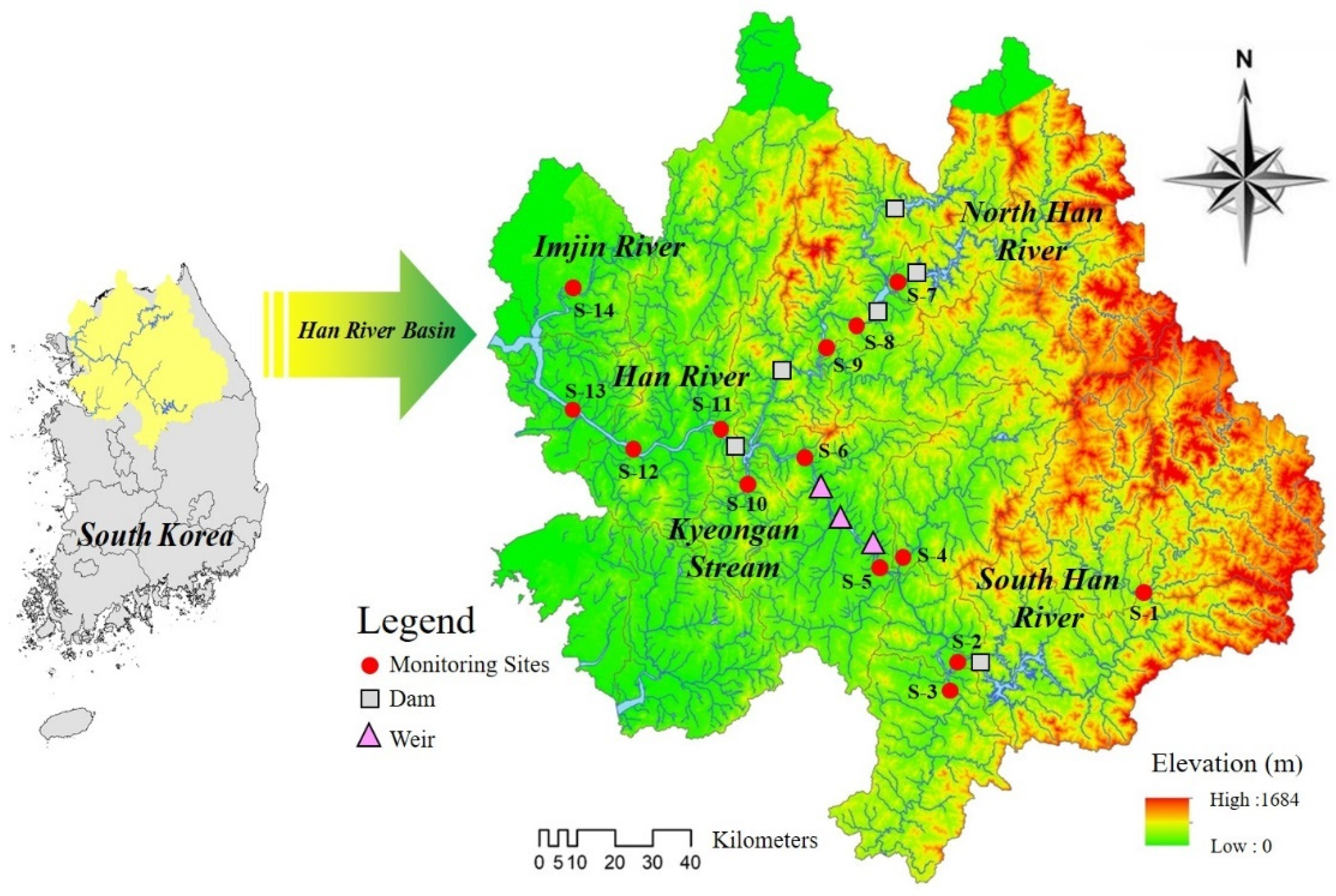
2.1. Study Area

The Han River is a result of the South Han River, originating from Mt. Daedeok in Taebaek city, Gangwon-do Province, that flows southwest and joins the North Han River and the Kyeongan stream at Yangsu-ri, Yangpyeong-gun, Gyeonggi-do Province, to form Lake Paldang. As the Han River flows towards Seoul through the Paldang Dam in Lake Paldang, tributaries, such as the Anyang stream, Tan stream, and Jungnang stream, are introduced, and the Han River joins the Imjin River at its estuary to flow into the West Sea [37]. The HRB (126°24′–129°02′ E, 36°30′–38°55′ N) is the largest basin in Korea with an area of 26.219 km2, accounting for approximately 27% of the entire country area [31,37]. The Han River is approximately 494 km long, and consists of 920 rivers and streams, including 19 national rivers and streams and 901 local rivers and streams [38]. The average annual precipitation in the HRB is approximately 1300 mm, and the basin witnesses a monsoon climate, with approximately 70% of the precipitation concentrated in summer (July–September) [31]. The annual average temperature ranges from 12.5 to 13.6 °C, which varies regionally [39]. In recent years, the average annual temperature has increased due to the acceleration of climate change; moreover, the length of summer has also increased due to seasonal influences, and the climatological length of winter has decreased from the natural length of the season. The Han River has a higher regime coefficient (1/393) than that of the Thames River (1/8), Rhine River (1/14), and Missouri River (1/75), thus indicating that it is subjected to severe flow fluctuations and is highly vulnerable to flooding [40,41]. Regarding the water use status in the HRB, domestic purposes represent the largest proportion (46.6%), followed by agricultural purposes (38.5%), and industrial purposes (14.9%) [42]. The land use status in the HRB comprises forests (68.9%), farmlands (14.9%), cities (8.3%), and other areas (7.9%) [38]. In this study, Yeongwol 2 (S-1), Chungju Dam (S-2), Dal Stream 4 (S-3), Seom River 4-1 (S-4), Gang Stream (S-5), Gangsang (S-6), Soyang River (S-7), Uiam Dam (S-8), Sambong-ri (S-9), Kyeongan Stream (S-10), Paldang Dam (S-11), Noryangjin (S-12), Gayang (S-13), and Imjin River (S-14) were selected as main water quality monitoring sites in the Han River water quality monitoring network operated by the Ministry of Environment (MOE) (Figure 1). The selected 14 sites were representative sites for river water quality monitoring and management in this study.

2.2. Water Quality Sampling Parameters and Analysis Methods

Water quality was sampled directly at 14 sites in the HBR for 10 years from January 2011 to December 2020. Sampling was performed every eight days on average when the direct influence of rainfall was insignificant and water quality was stable. Sampling points that represented the water quality and data uniformity were selected considering the safety of each site, such as the water flow and riverbed. The following 14 parameters were analyzed for water quality: water temperature (WT), pH, electrical conductivity (EC), dissolved oxygen (DO), biochemical oxygen demand (BOD), chemical oxygen demand (COD), total suspended solid (TSS), total nitrogen (TN), ammonia nitrogen (NH3-N), nitrate nitrogen (NO3-N), total phosphorous (TP), phosphate phosphorus (PO4-P), total organic carbon (TOC), and chlorophyll-a (Chl-a). WT, pH, EC, and DO were measured at each site using a multi-parameter water quality monitor (600 XLM, YSI, USA). Water samples for the other parameters were collected in 2 L polyethylene bottles (3 EA) that were washed with 0.1 N HNO3 solution; subsequently, the bottles were stored in an icebox at 4 °C or lower and transported to a laboratory for further analysis. Table S1 summarizes the sample analysis methods and the instruments used for the analyses. To evaluate the accuracy and reproducibility of the experiments, quality control was performed by measuring the accuracy, precision, and recovery rate of the results. The laboratory maintained reliable water quality analysis results through the certificate of international proficiency testing in the water quality field (WP289, WP291) hosted by the Environmental Resource Associate of the United States. In this study, sampling, preservation, and analysis of the collected water samples were conducted in accordance with the water pollution test standards of the MOE [43].

2.3. Data Treatment

Water samples (total 23,128) collected at the 14 monitoring sites (14 parameters × 1652 data matrix) were analyzed and the information was interpreted (Table S2). Field-collected data do not generally show normality due to the limited number of samples, survey time, and number of sampling sites. Thus, the Shapiro–Wilk normality test was used to assess the normality of the data and a significance level of p < 0.05 was used to assess statistical differences (Table S3) [44]. To avoid data errors, standardization for conversion into non-dimensional data with a mean of zero and a standard deviation of 1 (Z-score) was performed for the data of 23,128 samples [45].

2.4. Multivariate Statistical Analysis Techniques

To analyze the correlations between the water quality parameters, Pearson’s correlation coefficient (r) and the significance probability (p-value) were calculated using the open-source R software (ver. 4.1.0, comprehensive R archive network). The spatiotemporal variability of the water quality in the HRB was evaluated using multivariate statistical techniques (CA, FA, and PCA). In this study, standardized Z-scores were applied to correlation analysis, CA, FA, and PCA. The SPSS (Statistical Package of the Social Sciences, ver. 22 for Windows, USA) software was used for assessing the basic statistics, CA, FA, PCA, and APCS-MLR of the water quality data.
CA clusters large-capacity data into several groups with similar characteristics using a hierarchical method and identifies differences between the groups [9]. Squared Euclidean distance was applied to calculate the distance between the clusters, and Ward’s method was used to connect the clusters based on the variance of the entities constituting each cluster [11,46]. To improve the reliability and validity of CA, one-way analysis of variance (ANOVA) and post-hoc analysis was conducted.
FA reduces the dimensions of data comprising multiple variables while maintaining the variability present in the data as much as possible [3]. In this study, PCA, which extracts information from raw data using principal components (PCs) generated by performing dimension reduction for multivariate data, was performed. PCA, which analyzes the degree of interdependence between variables, is a linear combination of the eigenvectors of the covariance matrix calculated from standardized data [24]. Statistically insignificant variables were reduced through PCA, and the correlations between the parameters could be confirmed by extracting new varifactors (VFs) by rotating the acquired PC axes [3]. To rotate the PC axes, the varimax rotation method, which maximizes the variance by reducing the variables that are highly loaded on one factor, was applied [46]. Main factors that affected the water quality were interpreted by analyzing the commonality of VFs, which represent a newly created variable group through varimax rotation [20]. VFs include virtual potential variables that cannot be observed physically, whereas PCs are linear combinations of water quality variables that can be observed physically [47]. In this study, an eigenvalue of 1.0 or higher was considered in determining the number of PCs. To determine the applicability of the PCA data, Kaiser–Meyer–Olkin (KMO) and Bartlett’s Sphericity tests were conducted [24]. The KMO test measures the applicability of data that represents the general ratio of the variance, and PCA is possible if the ratio is 0.5 or higher [46]. Bartlett’s test represents whether a correlation matrix is a unit matrix, and PCA is possible if the significance level is less than 0.05 [48].
The non-standardized absolute principal component score (APCS) generated by PCA and the APCS-MLR model combined with the specific pollutant concentration measured through multiple linear regression (MLR) were used to calculate the contributions of potential pollution sources [49]. The contributions of potential pollution sources and those of the water quality variables selected for various pollution sources were calculated through regression coefficients [3,49].

3. Results and Discussion

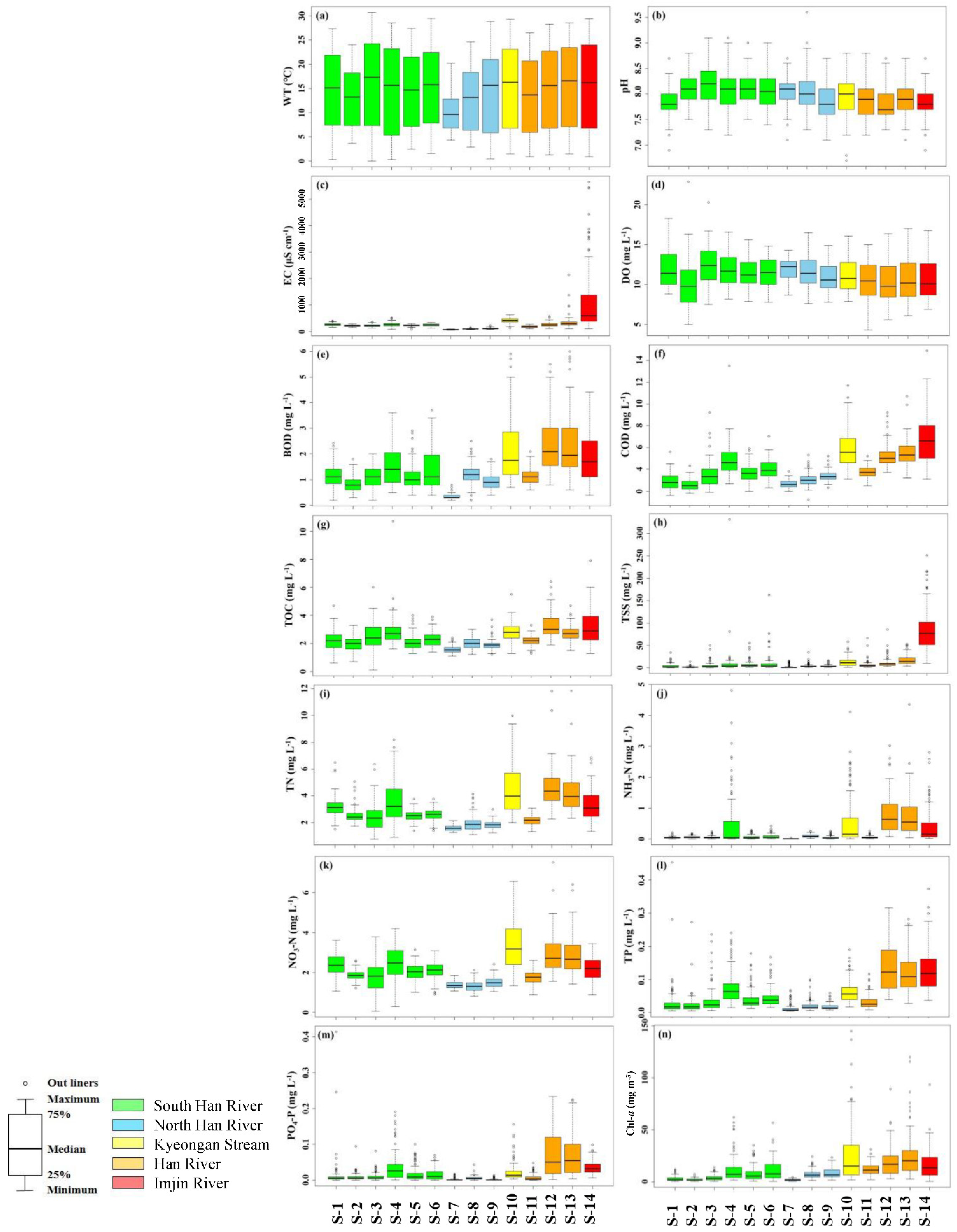
3.1. Spatiotemporal Variations in the Water Quality

Figure 2 summarizes the descriptive statistics (minimum, maximum, median values, and standard deviations) using a boxplot of the selected 14 water quality parameters surveyed at the monitoring sites. WT, EC, TSS, and Chl-a values, which are affected by seasons, exhibited large standard deviations. The pH of the HRB averaged 8.0 (weakly alkaline), and NH3-N, which is known to be toxic to aquatic plants, was 0.250 mg L−1 [50]. Ammonia nitrogen exists in aqueous solution as either ammonium ion or ammonia, depending on the pH of the solution, and it has been reported that NH3-N predominates at pH levels above 7 and NH4-N predominates at pH levels below 7 by equilibrium reaction [51]. WT, EC, COD, TSS, TP, and Chl-a concentrations showed evidently significant differences spatially (p < 0.05) (Figure S1).
At S-7, all parameters, except pH and DO, exhibited low concentrations possibly because of the influence of the effluent released during the operation of the Soyanggang Dam located upstream of the North Han River. S-14 exhibited higher concentrations of EC (1109 µS cm−1), COD (6.7 mg L−1), and TSS (84.6 mg L−1) than the other sites (Figure S1). This was because of the influence of the industrial wastewater generated from large industrial complexes (leather and dyeing factories) located in the HRB and the hydraulic characteristics caused by the tides at the Han River estuary [52,53]. S-12 showed high concentrations of TOC (3.4 mg L−1) and TP (0.138 mg L−1) possibly due to the high population density of the closely located large cities; additionally, the introduction of the Tan Stream and Anyang Stream, which are already affected by the effluents from public sewage treatment facilities, could have influenced the water quality [52]. Figure 3 shows the annual spatiotemporal variations in the water quality. WT, pH, DO, BOD, COD, TOC, TN, NH3-N, NO3-N, TP, PO4-P, and Chl-a showed high spatiotemporal variability.
The annual water quality in the HRB showed statistically significant (p < 0.05) temporal differences from precipitation, indicating a close relationship of the water quality with precipitation (Figure 3). In 2014, 2015, and 2019 when precipitation was relatively low, a deteriorated water quality was observed through the BOD, COD, TOC, TN, NH3-N, NO3-N, TP, PO4-P, and Chl-a parameters (Figure S2)

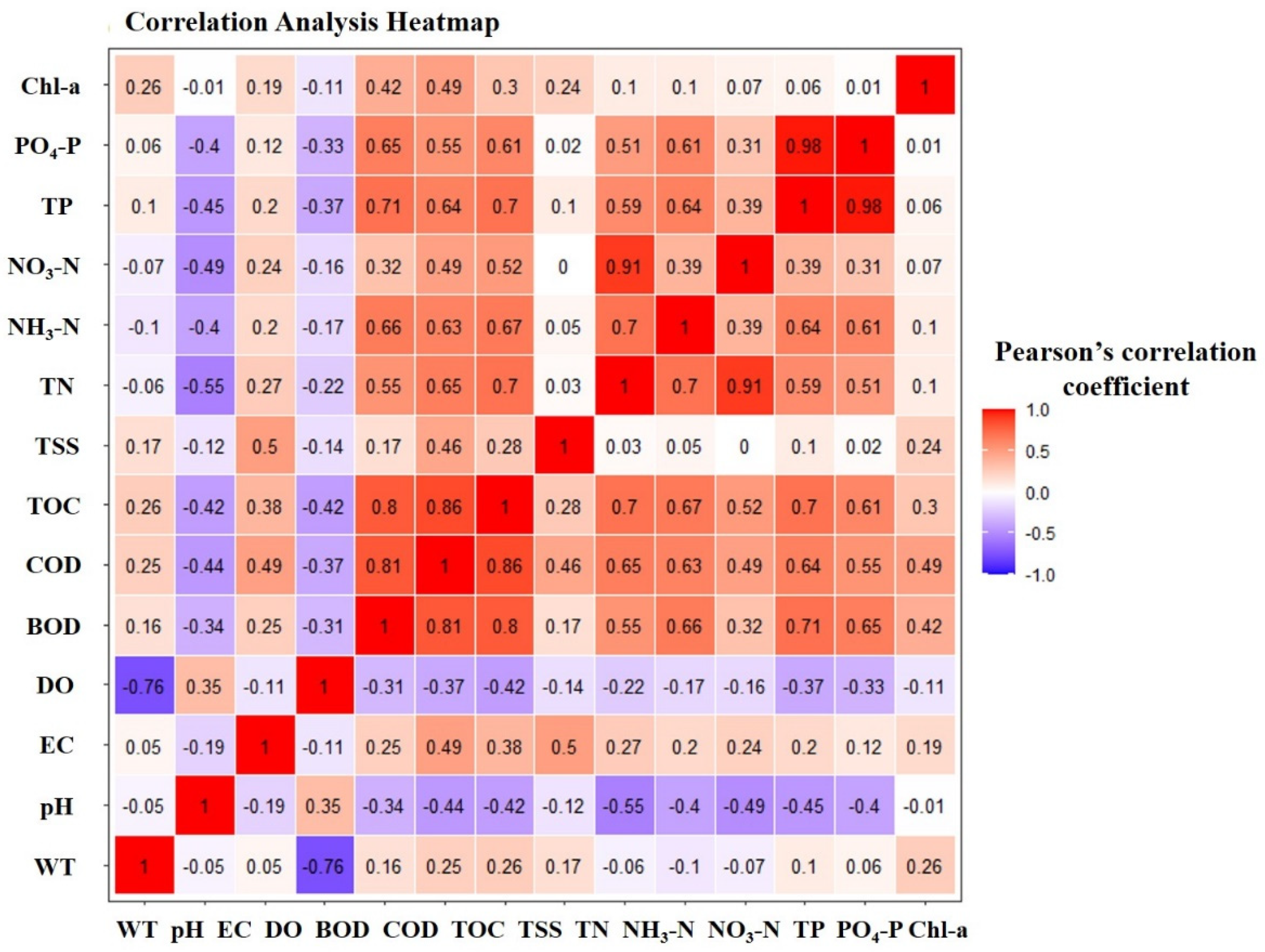
3.2. Correlation Analysis

To evaluate the relationships between water quality parameters in the HRB, correlation analysis was conducted on the 14 parameters (Figure 4). A statistically negative correlation was observed between WT and DO (r = −0.76, p < 0.05), thus indicating a seasonally dependent association, in which the solubility of oxygen decreases with the increase in the temperature [33]. Seasonally dependent parameters have been reported to majorly cause temporal variations in the water quality [3,24]. Moreover, TN, NH3-N, and NO3-N, which are not significantly associated with seasons, are contributors of anthropogenic sources in water catchment areas [54]. BOD showed statistically positive correlations (p < 0.05) with COD (r = 0.81), TOC (r = 0.80), and TP (r = 0.71), indicating that the water quality in the HRB is strongly correlated with organic matter and nutrient indicators. COD showed a statistically more significant level of correlation between TOC (r = 0.86, p<0.01) than BOD (r = 0.81, p < 0.01). Indeed, the biodegradability of organic substances occurs as a function of the rate and integrity of biodegradability by microorganisms [55]. The BOD/COD and COD/TOC ratios could be used to analyze the difficulty or ease of degradation of organic substances [56]. The BOD/COD and COD/TOC ratios in the HRB were 0.3 and 1.7, which are less than the COD/TOC ratio of three frequently found in wastewaters and were found to be less affected by anthropogenic sources [57]. TSS showed a statistically positive correlation (r = 0.46, p < 0.05) with COD but no statistically significant correlation with TN (r = 0.03, p > 0.05). A previous study on the correlations between water pollutants during summer rainfall indicated that TSS was strongly correlated with COD and TP and weakly correlated with TN [58]. In this study, Chl-a showed no statistically significant correlation (p > 0.05) with the nutrient concentrations of TN (r = 0.10) and TP (r = 0.06). This could be due to the average TN and TP concentrations in the HRB (3.580 and 0.105 mg L−1, respectively) no longer acting as limiting factors for algal growth as they exceed hypereutrophic states (1.500 and 0.100 mg L−1, respectively).

3.3. Cluster Analysis

To analyze the spatiotemporal similarity among the parameters in the HRB, the CA results were represented in a dendrogram (Figure 5). In spatial CA, the sites were classified into three statistically significant groups (Figure 5). Cluster 1 included the main sites of the South Han River (S-1, S-2, S-3, S-4, S-5, and S-6), Kyeongan Stream (S-10), and Han River (S-11, S-12, and S-13). Cluster 1 was located in rural and urban areas. The water quality characteristics in this region were affected by the point pollution source of discharge of domestic sewage, effluents from public sewage treatment facility, and livestock pollution sources [52,54]. Cluster 2 was composed of the main sites (S-8, S-9, and S-7) of the North Han River, and exhibited clean water quality characteristics due to the high proportion of forests and the effluent from dams (Soyanggang, Uiam, and Cheongpyeong dams). Cluster 3 included only the main site of the Imjin River (S-14), and exhibited high water quality characteristics under the hydraulic influence caused by the tidal action at the Han River estuary and the significant impact of the industrial wastewater discharged from large industrial complexes (Dongducheon city and Yangju city; 229 textile factories and 48 leather factories) [30,52,53]. The sites in the same groups had similar natural backgrounds and features that may be affected by similar pollution sources.
Therefore, the spatial water quality characteristics of the HRB could be considered to reflect the influence of similar geographic locations, land uses, natural background pollution sources, and sewage treatment plants [24,54]. To examine the validity of the CA results, the average difference between the three groups (Cluster 1, Cluster 2, and Cluster 3) was investigated. One-way ANOVA results showed that WT, EC, COD, TOC, TSS, and NO3-N concentration showed statistically significant differences (p < 0.05). Moreover, the post-hoc analysis results indicated that WT, pH, and DO in each group exhibited no water quality difference, but NO3-N in Cluster 1 and EC, BOD, COD, TSS, NH3-N, TP, and Chl-a in Cluster 3 showed statistically significant differences (p < 0.05).
The mean and standard deviation values of the parameters that were calculated to compare the water quality characteristics between the groups created by the CA were summarized in Table S4. Compared with the water quality of Cluster 1 and Cluster 3, the water quality of Cluster 2 corresponded to a low pollution region (LPR) having low concentrations of organic pollutants and nutrient indicators. The water quality of Cluster 3 exhibited high EC, COD, TSS, and TP values, and corresponded to high pollution region (HPR). The water quality of Cluster 1 showed high concentrations for nitrogen-related and Chl-a parameters, and corresponded to a moderate pollution region (MPR). Previous studies reported that forest areas show clean water, whereas rural areas show high nitrogen concentrations in the water [59,60]. Thus, the water quality of each group created by CA could represent the water quality of the target basin and can be used to evaluate the spatial water quality [3].
In temporal CA, 12 months were classified into two statistically significant groups. Cluster 1, corresponding to the dry season of South Korea, was composed of January, February, March, April, May, June, October, and November, while Cluster 2, corresponding to the rainy season of South Korea, included July, August, September, and October. The temporal variability of the HRB was classified into these two groups because precipitation and hydraulic/hydrological characteristics influenced water quality. To examine the validity of the temporal CA results, one-way ANOVA was conducted to analyze the differences between the two groups. The results indicated a statistically significant difference (p < 0.05) between the seasons.
Further, the CA results provided reliable information on the spatiotemporal characteristics inherent in the HRB. In addition, each group classified based on the characteristics of surrounding pollution sources and the degree of river water pollution could represent the water quality of the target area. Moreover, the CA results can assist in proposing sampling strategies that can reduce the sampling frequency at monitoring sites and the number of sites, thereby reducing the costs of sampling [2,3,47]. Thus, to implement measures to manage the water quality in the HRB in the future, proposing water quality management measures for groups with similar water quality characteristics was judged to be more efficient than proposing management measures for each river or site.

3.4. Factor Analysis and Principal Component Analysis

To identify variables and factors that affect the variability of water quality in the HRB, FA/PCA was conducted in the MPR, LPR, and HPR. The KMO test results for the FA/PCA model were higher than 0.5 in the MPR (0.719), LPR (0.745), and HPR (0.758); additionally, the Bartlett‘s test result was 0.000 (p < 0.05), indicating the suitability of the FA/PCA method [61]. In this study, the number of PCs was determined based on an eigenvalue of 1.0 or higher and was demonstrated on a Scree plot (Figure S3). The Scree plot is used to identify the number of PCs that must be maintained to understand the overall data structure [9]. Table 1 shows the loading value results in varimax rotation for standardized data. Explanations on all variances, the amount of data that could be analyzed by each VF, and the cumulative amount were confirmed. The maximum variance could be explained by the extracted VF1; however, the proportion of variances that could be explained gradually decreased. Factors were analyzed as >0.75 (strong), 0.75–0.50 (moderate), and 0.50–0.30 (weak) according to the loading value of the VFs [45]. Figure 6 shows a plot for the 14 variables from varimax rotated PCA. These newly generated principal components were orthogonal, and each component could explain part of the variance of the whole dataset; thus, principal components were identified as pollution sources [62].
The PCA results for water quality data of the LPR showed that 80.1% of the total variance could be explained with four PCs. VF1 that contributed to 25.8% of the total variance was correlated to BOD, COD, TOC, and Chl-a, which could be interpreted as the influence of organic matter and algal growth (loading >0.60). VF2 that contributed to 22.8% of the total variance was correlated to EC, TN, NH3-N, and NO3-N, which could be interpreted as the influence of nitrogen (loading >0.60). Further, VF3 that contributed to 15.9% of the total variance was correlated to pH, TP, and PO4-P, which could be interpreted as the influence of phosphorus present due to the river metabolism (loading >0.60). Finally, VF4 that contributed to 15.6% of the total variance was correlated to WT and DO, which could be interpreted as a seasonal influence (loading >0.60).
Based on the water quality data of the MPR, the PCA results showed that 74.1% of the total variance could be explained with four PCs. VF1 contributing to 26.6% of the total variance was correlated to COD, Chl-a, TOC, BOD, and TSS, which could be interpreted as the significant influence of organic matter due to the increase in the river flow during rainfall (loading >0.40). VF2 that contributed to 24.3% of the total variance was correlated to TN, WT, EC, DO, NH3-N, and NO3-N, which could have been influenced by nitrogen due to seasonality (loading >0.60). VF3 that contributed to 14.8% of the total variance was correlated to TP and PO4-P, which could be interpreted as the influence of phosphorus (loading >0.80). Finally, VF4 that contributed to 8.4% of the total variance was correlated to pH, which could be interpreted as the influence of the river metabolism (loading >0.90).
Based on the HPR water quality data, the PCA results showed that 72.7% of the total variance could be explained with three PCs. VF1 that contributed to 30.0% of the total variance was correlated to BOD, COD, TOC, TSS, TP, PO4-P, and Chl-a, which could be interpreted as the influence of the phosphorus-based sediments accumulated at the bottom of the river water body and organic matter (loading >0.60). VF2 contributing to 29.7% of the total variance was correlated to WT, DO, TN, NH3-N, and NO3-N, which could be interpreted as the influence of nitrogen due to seasonality (loading >0.70). VF3 contributing to 13.0% of the total variance was correlated to pH and EC, which could be interpreted as the influence of the river metabolism (loading >0.60).
The results of the component matrix through varimax rotation showed that the main factors that affected the HRB water quality varied depending on the pollution region, but BOD, COD, TOC, and Chl-a were commonly extracted from VF1, indicating the importance of managing organic matter and algal loads. To develop prediction models for main factors according to the FA/PCA results, stepwise MLR analysis was conducted using VFs as dependent variables and factor loading scores as independent variables (Table 2). Except for the VF3 prediction model of the MPR, the coefficient of determination (R2) was higher than 0.700 for all the other models, indicating high explanatory power. The significance probability of the F statistic was also statistically significant (p < 0.05). Therefore, using prediction models facilitates the determination of the influence of environmental factors on the water quality in the HRB, and prevention of water pollution in advance.

3.5. Analysis of the Source Contribution Using APCS-MLR

After determining the number and characteristics of potential pollution sources using PCA, the contribution of each source was quantified using the MLR of the sample concentrations for APCS [63,64]. Table 3 shows the contribution of each source to the physicochemical parameters of the LPR, MPR, and HPR. In this study, the contributions of unidentified sources (UIS) were also considered and expressed (Table 3). R2 was higher than 0.5, indicating a relatively excellent correlation between the observed and predicted values and the possibility of reliable evaluation for the allocation of pollution sources [46,63].
The LPR was significantly affected by domestic sewage from households and phytoplankton growth (VF1, 25.4%). Further, organic matter (BOD, 40.2%; COD, 26.0%; and TOC, 26.0%) and algae (Chl-a, 36.9%) exhibited significant contributions. In addition, the nonpoint pollution sources caused by agricultural activities (VF2) accounted for 24.2% of all pollution sources, and were contributed by NO3-N (38.3%), NH3-N (29.6%), and TN (28.8%). PO4-P (45.4%), TP (30.5%), and pH (30.3%) contributed to the point pollution sources caused by the discharge of domestic sewage and industrial wastewater (VF3, 23.8%). WT (36.2%) and TSS (27.7%) contributed to seasonal influences (VF4, 20.9%).
The MPR was significantly affected by domestic sewage and phytoplankton growth (VF1, 28.7%), which were contributed by organic matter (TOC, 52.3%; COD, 37.4%; and BOD, 32.0%; TSS, 27.2%) and Chl-a (36.9%). The influence of the nonpoint pollution sources caused by agricultural activities and seasonality represented 23.5% (VF2) of all pollution sources, and were contributed by NH3-N (43.7%), TN (30.3%), NO3-N (29.4%), WT (31.0%), and DO (23.2%). In addition, PO4-P (38.2%) and TP (33.4%) contributed to the point pollution sources caused by the discharge of domestic sewage and industrial wastewater (VF3, 22.6%). Furthermore, pH (31.5%) and EC (28.7%) contributed to the river metabolism (VF4, 20.0%). For spatial variation, the mean pH value was high in MPR. The natural background pH value of MPR has been shown to be ≥7 for Ca2+ and HCO3- type water associated with limestone soils in the acid region [65]. Furthermore, a higher average value of NH3-N was found in the MPR, which suggested that the eutrophication might be a serious water quality problem in the region.
The HPR was significantly affected by the point pollution sources caused by industrial and domestic sewage (VF1, 33.8%), and were contributed by BOD (55.9%), TP (54.6%), PO4-P (52.2%), TOC (51.5%), COD (51.3%), and TSS (49.6%). The influence of the nonpoint pollution sources caused by agricultural activities and seasonality accounted for 31.1% (VF2) of all pollution sources, and were contributed by nitrogen-related parameters (NH3-N, 62.3%; NO3-N, 52.0%; and TN. 36.7%), WT (51.0%), and DO (32.9%). As shown in Table 3, UIS ranged from 0.01% to 16.8% in the three pollution regions, contributing to river water pollution for all water quality parameters. This may be because pollutants originate from mixed and complicated sources, which make source identification using the APCS-MLR approach particularly challenging [46,63]. Based on the information extracted from PCA and the contribution calculated from APCS-MLR, more effective water quality management plans can be implemented to critical pollution zones to ensure the efficient and sustainable utilization of resources [66].

3.6. Strengths and Limitations

This study has several strengths and limitations. First, the study demonstrates that the multivariate statistical techniques and APCS-MLR model is an efficient exploratory tool for understanding spatial and temporal variations in water quality as well as identifying and apportioning pollution sources for efficient water management in the HRB. Second, this study demonstrates the feasibility and reliability of the combined use of these methods in water environment research. Furthermore, the results would be beneficial to future policies pertaining to water environment protection and water resources management. Third, the difference in potential pollution level was quantitatively presented for appropriate water quality management in the basin according to the pollution level, and the primary pollution sources were identified. These results provide information that can help prioritize water quality improvement in the HRB, where water quality is deteriorating due to various causes. However, some limitations should be considered when interpreting our findings. First, water quality samples at the 14 sites the water quality measurement network may not reflect the water quality concentrations of the entire HRB. Although we collected samples at the same location and time, we could not collect mineralogical and heavy metal data. Second, the effects of point pollution sources in the basin population, livestock, and industry and astigmatism in the land system are not considered. These factors must be focused on in future research. Therefore, additional research is needed to accurately assess the volatility of water quality variables and unidentified sources of pollution that could not be measured in the study. Moreover, the comprehensive results of this study provide deeper insights into the major pollution sources in the HRB; this can be beneficial to water quality managers and policy makers and help them prioritize water quality improvement.

4. Conclusions

Multivariate statistical analysis approaches and APCS-MLR were used in this study to assess the spatiotemporal variability of water quality and contributions of various probable pollution sources in the HRB, South Korea. Fourteen water quality parameters surveyed at 14 sites in the water quality monitoring network of the MOE were analyzed from 2011 to 2020. Water quality in the HRB showed statistically significant positive correlations with BOD and TP (r = 0.71, p < 0.05), showing that organic matter and nutrient indicators have a strong relationship. Information from the CA-clustered group could be utilized to minimize the spatiotemporal characteristics without losing a lot of data. Spatial CA classified the 14 monitoring sites into three groups (LPR, MPR, and HPR) based on similar water pollution (natural and anthropogenic) characteristics. Temporal CA split 12 months into two time periods (dry and wet seasons) and reflected precipitation and hydraulic/hydrological characteristics of water quality. FA/PCA was used to identify four potential factors that accounted for 80.1% and 74.1% of the total variance in the LPR and MPR, respectively, and three potential factors that accounted for 72.7% of the total variance in the HPR. In the LPR, MPR, and HPR, the APCS-MLR model quantitatively demonstrated the disparities in the contributions of potential pollution sources. Organic matter and phytoplankton growth (VF1, 25.4%), organic matter and seasonal influence (VF1, 28.7%), and the point pollution sources caused by the discharge of domestic sewage and industrial wastewater (VF1, 33.8%) were found to be the main pollution sources for the LPR, MPR, and HPR, respectively.
In the HRB, South Korea, this study demonstrated that multivariate statistical and the APCS-MLR modeling techniques could be used for efficient understanding of the spatiotemporal variations in water quality and identification of potential pollution sources for efficient water quality management.

Supplementary Materials

The following are available online at https://www.mdpi.com/article/10.3390/agronomy11122469/s1, Figure S1: Spatial variation of water quality parameters (a) WT, (b) EC, (c) COD, (d) TSS, (e) TP, and (f) Chl-a in the monitoring sites of Han River Basin, South Korea, Figure S2: Precipitation and discharge in the Han River Basin from 2011 to 2020, Figure S3: Eigenvalue change with number of principal component (a) MPR, (b) LPR, (c) HPR, Table S1: Information on analytical methods and instruments, Table S2: Summary descriptive statistics of water quality parameters between 2011 and 2020, Table S3: Results of Shapiro–Wilk test for normality, Table S4: Descriptive statistics of water quality variables in different clusters in the Han River Basin.

Author Contributions

Conceptualization, Y.-C.C. and J.-K.I.; methodology, H.C.; software, Y.-C.C.; validation, Y.-C.C. and H.C.; formal analysis, Y.-C.C.; investigation, H.C., S.-H.K. and S.-J.Y.; resources, S.-J.Y.; data curation, Y.-C.C.; writing—original draft preparation, Y.-C.C. and J.-K.I.; writing—review and editing, Y.-C.C., H.C., S.-H.K., S.-J.Y. and J.-K.I.; visualization, Y.-C.C. and H.C.; supervision, S.-J.Y.; project administration, S.-H.K.; funding acquisition, S.-J.Y. All authors have read and agreed to the published version of the manuscript.

Funding

This research was supported by the National Institute of Environmental Research (NIER) (grant number NIER-2021-01-01-134), funded by the Ministry of Environment (MOE) of the Republic of Korea.

Data Availability Statement

Not applicable.

Conflicts of Interest

The authors declare no conflict of interest.

References

  1. Pejman, A.H.; Nabi Bidhendi, G.R.; Karbassi, A.R.; Mehrdadi, N.; Esmaeili Bidhendi, M. Evaluation of spatial and seasonal variations in surface water quality using multivariate statistical techniques. Int. J. Environ. Sci. Technol. 2009, 6, 467–476. [Google Scholar] [CrossRef] [Green Version]
  2. Simeonov, V.; Stratis, J.A.; Samara, C.; Zachariadis, G.; Voutsa, D.; Anthemidis, A.; Sofoniou, M.; Kouimtzis, T. Assessment of the surface water quality in Northern Greece. Water Res. 2003, 37, 4119–4124. [Google Scholar] [CrossRef]
  3. Singh, K.P.; Malik, A.; Mohan, D.; Sinha, S. Multivariate statistical techniques for the evaluation of spatial and temporal variation in water quality of Gomti River (India). Water Res. 2004, 38, 3980–3992. [Google Scholar] [CrossRef] [PubMed]
  4. Martinez-Tavera, E.; Rodriguez-Espinosa, P.F.; Shruti, V.C.; Sujitha, S.B.; Morales-Garcia, S.S.; Munoz-Sevilla, N.P. Monitoring the seasonal dynamics of physicochemical parameters from Atoyac River basin (Puebla), Central Mexico: Multivariate approach. Environ. Earth Sci. 2017, 76, 95. [Google Scholar] [CrossRef] [Green Version]
  5. Zhang, Q.; Li, Z.; Zeng, G.; Li, J.; Fang, Y.; Yuan, Q.; Wang, Y.; Ye, F. Assessment of surface water quality using multivariate statistical techniques in red soil hilly region: A case study of Xiangjiang watershed, China. Environ. Monit. Assess. 2009, 152, 123–131. [Google Scholar] [CrossRef] [PubMed]
  6. Anteneh, Y.; Zeleke, G.; Gebremariam, E. Assessment of surface water quality in Legedadie and Dire catchments, Central Ethiopia, using multivariate statistical analysis. Acta Ecol. Sin. 2018, 38, 81–95. [Google Scholar] [CrossRef]
  7. Najafpour, S.; Alkarkhi, A.F.M.; Kadir, M.O.A.; Najafpour, G.D. Evaluation of spatial and temporal variation in river water quality. Int. J. Environ. Res. 2008, 2, 349–358. [Google Scholar]
  8. Khadka, R.B.; Khanal, A.B. Environmental management plan (EMP) for Melamchi water supply project, Napal. Environ. Monit. Assess. 2008, 146, 225–234. [Google Scholar] [CrossRef] [Green Version]
  9. Xu, G.; Li, P.; Lu, K.; Tantai, Z. Seasonal change in water quality and its main influencing factors in the Dan River basin. Catena 2019, 173, 131–140. [Google Scholar] [CrossRef]
  10. Mouri, G.; Takizawa, S.; Oki, T. Spatial and temporal variation in nutrient parameters in stream water in a rural-urban catchment, Shikoku, Japan: Effects of land cover and human impact. J. Environ. Manag. 2011, 92, 1837–1848. [Google Scholar] [CrossRef]
  11. Varol, M.; Gokot, B.; Bekleyen, A.; Sen, B. Spatial and temporal variations in surface water quality of the dam reservoirs in the Tigris River basin, Turkey. Catena 2012, 92, 11–21. [Google Scholar] [CrossRef]
  12. Sargaonkar, A.; Deshpande, V. Development of an overall index of pollution for surface water based on a general classification scheme in Indian context. Environ. Monit. Assess. 2003, 89, 43–67. [Google Scholar] [CrossRef]
  13. Strobl, R.O.; Robillard, P.D. Network design for water quality monitoring of surface freshwaters: A review. J. Environ. Manag. 2008, 87, 639–648. [Google Scholar] [CrossRef]
  14. Pesce, S.F.; Wunderlin, D.A. Use of water quality indices to verify the impact of Cordoba city (Argentina) on Suquia River. Water Res. 2000, 34, 2915–2926. [Google Scholar] [CrossRef]
  15. Bordalo, A.A.; Nilsumranchit, W.; Chalermwat, K. Water quality and uses of the Bangpakong River (Eastern Thailand). Water Res. 2001, 35, 3635–3642. [Google Scholar] [CrossRef]
  16. Nagaraju, A.; Sreedhar, Y.; Thejaswi, A.; Sayadi, M.H. Water quality analysis of the Rapur area, Andhra Pradesh, South India using multivariate techniques. Appl. Water Sci. 2017, 7, 2767–2777. [Google Scholar] [CrossRef] [Green Version]
  17. Karim, B.; Taha, F.M. Using principal component analysis to monitor spatial and temporal changes in water quality. J. Hazard. Mater. 2003, B100, 179–195. [Google Scholar]
  18. Said, M.E.S.; Ali, A.M.; Borin, M.; Abd, S.K.; Aldosari, A.A.; Khalil, M.M.N.; Abdel, M.K. On the use of multivariate analysis and land evaluation for potential agricultural development of the northwestern Coast of Egypt. Agronomy 2020, 10, 1318. [Google Scholar] [CrossRef]
  19. Tadano, S.; Chiyapo, G.; Ishimoto, Y.; Konaka, T.; Mazereku, C.; Tsujimoto, H.; Akashi, K. Multivariate analysis of seed chemical diversity among Jatropha curcas in Botswana. Agronomy 2021, 11, 1570. [Google Scholar] [CrossRef]
  20. Helena, B.; Pardo, R.; Vega, M.; Barrado, E.; Fernandez, J.M.; Fernandez, L. Temporal evolution of groundwater composition in an alluvial aquifer (Pisuerga River, Spain) by principal component analysis. Water Res. 2000, 34, 807–816. [Google Scholar] [CrossRef]
  21. Ioele, G.; De Luca, M.; Grande, F.; Durante, G.; Trozzo, R.; Crupi, C.; Ragno, G. Assessment of Surface Water Quality Using Multivariate Analysis: Case Study of the Crati River, Italy. Water 2020, 12, 2214. [Google Scholar] [CrossRef]
  22. Alberto, W.D.; Pilar, D.M.D.; Valeria, A.M.; Fabiana, P.S.; Cecilia, H.A.; Angeles, B.M.D.L. Pattern recognition techniques for the evaluation of spatial and temporal variations in water quality. A case study: Suquia River basin (Cordoba-Argentina). Water Res. 2001, 35, 2881–2894. [Google Scholar] [CrossRef]
  23. Sundaray, S.K.; Panda, U.C.; Nayak, B.B.; Bhatta, D. Multivariate statistical techniques for the evaluation of spatial and temporal variation in water quality of the Mahanadi river-estuarine system (India)—A case study. Environ. Geochem. Health 2006, 28, 317–330. [Google Scholar] [CrossRef]
  24. Shrestha, S.; Kazama, F. Assessment of surface water quality using multivariate statistical techniques: A case study of the Fuji River Basin, Japan. Environ. Model. Soft. 2007, 22, 464–475. [Google Scholar] [CrossRef]
  25. Kannel, P.R.; Lee, S.; Kanel, S.R.; Khan, S.P. Chemometric application and assessment of monitoring locations of an urban river system. Anal. Chim. Acta 2007, 582, 390–399. [Google Scholar] [CrossRef]
  26. Zhang, Y.; Guo, F.; Meng, W.; Wang, X.Q. Water quality assessment and source identification of Daliao river basin using multivariate statistical methods. Environ. Monit. Assess. 2009, 152, 105–121. [Google Scholar] [CrossRef] [PubMed]
  27. Kim, M.A.; Lee, J.K.; Zoh, K.D. Evaluation of the Geum River by multivariate analysis: Principle component analysis and factor analysis. J. Korean Soc. Water Environ. 2007, 23, 161–168. [Google Scholar]
  28. Park, S.M.; Kazama, F.; Lee, S.H. Assessment of water quality using multivariate statistical techniques: A case study of the Nakdong River Basin, Korea. Environ. Eng. Res. 2014, 19, 197–203. [Google Scholar] [CrossRef]
  29. Jung, K.Y.; Lee, K.L.; Im, T.H.; Lee, I.J.; Kim, S.; Han, K.Y.; Ahn, J.M. Evaluation of water quality for the Nakdong River watershed using multivariate analysis. Environ. Technol. Innov. 2016, 5, 67–82. [Google Scholar] [CrossRef]
  30. Lee, K.H.; Kang, T.W.; Ryu, H.S.; Hwang, S.H.; Kim, K. Analysis of spatiotemporal variation in river water quality using clustering techniques: A case study in the Yeongsan River, Republic of Korea. Environ. Sci. Pollut. Res. 2020, 27, 29327–29340. [Google Scholar] [CrossRef]
  31. Chang, H.J. Spatial Analysis of Water Quality Trends in the Han River Basin, South Korea. Water Res. 2008, 42, 3285–3304. [Google Scholar] [CrossRef] [PubMed]
  32. Park, T.J.; Lee, S.H.; Lee, M.S.; Lee, J.K.; Lee, S.H.; Zoh, K.D. Occurrence of Microplastics in the Han River and Riverine Fish in South Korea. Sci. Total Environ. 2020, 708, 134535. [Google Scholar] [CrossRef] [PubMed]
  33. Cho, Y.C.; Choi, H.M.; Ryu, I.G.; Kim, S.H.; Shin, D.S.; Yu, S.J. Assessment of water quality in the lower reaches Namhan River by using statistical analysis and water quality index (WQI). J. Korean Soc. Water Environ. 2021, 37, 114–127. [Google Scholar]
  34. Collins, A. The Global Risks Report 2019; World Economic Forum: Geneva, Switzerland, 2018; Volume 6. [Google Scholar]
  35. Rifkin, J. The Global Green New Deal. Why the Fossil Fuel Civilization Will Collapse by 2028, and the Bold Economic Plan to Save Life on Earth; St. Martin’s Press: New York, NY, USA, 2019. [Google Scholar]
  36. Chang, H.J. Spatial and Temporal Variations of water Quality in the Han River and Its Tributaries, Seoul, Korea, 1993–2002. Water Air Soil Pollut. 2005, 161, 267–284. [Google Scholar] [CrossRef]
  37. Thom, T.L.; Li, L.; Kyung, S.J. Evaluation of Multi-Satellite Precipitation Products for Streamflow Simulations: A Case Study for the Han River in the Korean Peninsula, East Asia. Water 2018, 10, 642. [Google Scholar]
  38. Park, S.R.; Hwang, S.J.; An, K.J.; Lee, S.W. Identifying Key Watershed Characteristics That Affect the Biological Integrity of Streams in the Han River Watershed, Korea. Sustainability 2021, 13, 3359. [Google Scholar] [CrossRef]
  39. Ministry of Environment (MOE). National Water Environment Management Plan for Han River Basin; Han River Basin Environmental Office: Yangpyeong-Gun, Korea, 2015. [Google Scholar]
  40. Lee, K.S.; Ryu, J.K.; Ahn, S.J. Change of regime coefficient due to dredging and dam construction. J. Korean Environ. Dredg. Soc. 2014, 4, 30–38. [Google Scholar]
  41. Ji, U.; Jang, E.K.; Yeo, W.K. Channel-forming discharge evaluation for rivers with high coefficients of river regime. J. Korean Soc. Civ. Eng. 2011, 31, 361–367. [Google Scholar]
  42. Kim, K.S.; Na, Y.M. The present state and improvement of water quality of Han River. J. Korean Soc. Environ. Eng. 2011, 29, 1169–1178. [Google Scholar]
  43. Ministry of Environment (MOE). Standard Methods of Water Sampling and Analysis; Ministry of Environment: Incheon, Korea, 2011.
  44. Kumar, M.; Ramanathan, A.; Rao, M.S.; Kumar, B. Identification and evaluation of hydrogeochemical processes in the groundwater environment of Delhi, India. Environ. Geol. 2006, 50, 1025–1039. [Google Scholar] [CrossRef]
  45. Liu, C.W.; Linn, K.H.; Kuon, Y.M. Application of factor analysis in the assessment of groundwater quality in a black foot disease area in Taiwan. Sci. Total Environ. 2003, 313, 77–89. [Google Scholar] [CrossRef]
  46. Zhang, H.; Li, H.; Yu, H.; Cheng, S. Water quality assessment and pollution source apportionment using multi-statistic and APCS-MLR modeling techniques in Min River Basin, China. Environ. Sci. Pollut. Res. 2020, 27, 41987–42000. [Google Scholar] [CrossRef]
  47. Varekar, V.; Karmakar, S.; Jha, R. Seasonal rationalization of river water quality sampling locations: A comparative study of the modified Sander and multivariate statistical approaches. Environ. Sci. Pollut. Res. 2016, 23, 2308–2328. [Google Scholar] [CrossRef] [PubMed]
  48. Li, Q.; Zhang, H.; Guo, S.; Fu, K.; Liao, L.; Xu, Y.; Cheng, S. Groundwater pollution source apportionment using principal component analysis in a multiple land-use area in southwestern China. Environ. Sci. Pollut. Res. 2019, 27, 9000–9011. [Google Scholar] [CrossRef]
  49. Liu, L.; Dong, Y.; Kong, M.; Zhou, J.; Zhao, H.; Tang, Z.; Wang, Z. Insights into the long-term pollution trends and sources contributions in Lake Taihu, China using multi-statistics analysis models. Chemosphere 2019, 242, 125272. [Google Scholar]
  50. Dyer, S.D.; Peng, C.; McAvoy, D.C.; Fendinger, N.J.; Masscheleyn, P.; Castillo, L.V.; Lim, J.M.U. The influence of untreated wastewater to aquatic communities in the Balatuin River, The Philippines. Chemosphere 2003, 52, 43–53. [Google Scholar] [CrossRef]
  51. Me Metcalf, L.; Eddy, H.P. Wastewater Engineering, 3rd ed.; McGraw-Hill, Inc.: New York, NY, USA, 2003. [Google Scholar]
  52. Kim, Y.Y.; Lee, S.J. Evaluation of water quality for the Han River tributaries using multivariate analysis. J. Korean Soc. Environ. Eng. 2011, 33, 501–510. [Google Scholar] [CrossRef]
  53. Choi, O.Y.; Kim, K.H.; Han, I.S. A study on the spatial strength and cluster analysis at the unit watershed for the management of total maximum daily loads. J. Korean Soc. Water Environ. 2015, 31, 700–714. [Google Scholar] [CrossRef] [Green Version]
  54. Wang, X.; Cai, Q.; Ye, L.; Qu, X. Evaluation of spatial and temporal variation in stream water quality by multivariate statistical techniques; A case study of the Xiangxi River Basin, China. Quat. Int. 2012, 282, 137–144. [Google Scholar] [CrossRef]
  55. Sponza, D.T. Application of toxicity tests into discharge of the pulp-paper industry in Turkey. Ecotoxicol. Environ. Saf. 2003, 54, 74–86. [Google Scholar] [CrossRef]
  56. Emmanuel, E.; Keck, G.; Blanchard, J.M.; Vermande, P.; Perrodin, Y. Toxicological effects of disinfection using sodium hypochlorite on aquatic organisms and its contribution to AOX formation in hospital wastewater. Environ. Int. 2004, 30, 891–900. [Google Scholar] [CrossRef]
  57. Seiss, M.; Gahr, A.; Niessner, R. Improved Aox degradation in UV oxidative waste water treatment by dialysis with nanofiltration mem membrane. Water Res. 2001, 35, 3242–3248. [Google Scholar] [CrossRef]
  58. Jeon, J.H.; Yoon, C.G.; Ham, J.H. Analysis of relationships among the pollutant concentrations in non-urban area. Korean J. Ecol. Environ. 2001, 34, 215–222. [Google Scholar]
  59. Wan, B.; Cai, S.; Li, H.; Yang, G.; Li, Z.; Nie, X. Inferring land use and land cover impact on stream water quality using a Bayesian hierarchical modeling approach in the Xitiaoxi River watershed, China. J. Environ. Manag. 2014, 133, 1–11. [Google Scholar] [CrossRef] [PubMed]
  60. Allan, J.D. Landscapes and riverscapes: The influence of land use on stream ecosystems. Annu. Rev. Ecol. Evol. Syst. 2004, 35, 257–284. [Google Scholar] [CrossRef] [Green Version]
  61. Bernard, P.; Antoine, L.; Bernard, L. Principal component analysis an appropriate tool for water quality evaluation and management application to a tropical lake system. Ecol. Model. 2004, 178, 295–311. [Google Scholar]
  62. Zhou, F.; Guo, H.; Liu, L. Quantitative identification and source apportionment of anthropogenic heavy metals in marine sediment of Hong Kong. Environ. Geol. 2007, 53, 295–305. [Google Scholar] [CrossRef]
  63. Gholizadeh, M.H.; Melesse, A.M.; Reddi, L. Water quality assessment and apportionment of pollution sources using APCS-MLR and PMF receptor modeling techniques in three major rivers of South Florida. Sci. Total Environ. 2016, 566, 1552–1567. [Google Scholar] [CrossRef] [PubMed]
  64. Lv, J. Multivariate receptor models and robust geostatistics to estimate source apportionment of heavy metals in soils. Environ. Pollut. 2019, 244, 72–83. [Google Scholar] [CrossRef] [PubMed]
  65. Chen, P.; Li, L.; Zhang, H. Spatio-temporal variations and source apportionment of water pollution in Danjiangkou Reservoir Basin, Central China. Water 2015, 7, 2591–2611. [Google Scholar] [CrossRef] [Green Version]
  66. Yang, L.; Mei, K.; Liu, X.; Wu, L.; Zhang, M.; Xu, J.; Wang, F. Spatial distribution and source apportionment of water pollution in different administrative zones of Wen-Rui-Tang (WRT) river watershed, China. Environ. Sci. Pollut. Res. 2013, 20, 5341–5352. [Google Scholar] [CrossRef] [PubMed]
Figure 1. Map showing the water quality monitoring sites in the Han River Basin, South Korea.
Agronomy 11 02469 g001
Figure 2. Basic descriptive statistics of water quality parameters between 2011 and 2020 in the Han River Basin. (a) WT, (b) pH, (c) EC, (d) DO, (e) BOD, (f) COD, (g), TOC, (h) TSS, (i) TN, (j) NH3-N, (k) NO3-N, (l) TP, (m) PO4-P, (n) Chl-a.
Agronomy 11 02469 g002
Figure 3. Temporal and spatial variation of water quality parameters in the monitoring sites of Han River Basin, South Korea.
Agronomy 11 02469 g003
Figure 4. Pearson correlation coefficient matrix between water quality parameters in the Han River Basin, South Korea.
Agronomy 11 02469 g004
Figure 5. Dendrogram showing hierarchical (a) spatial and (b) temporal clustering according to Ward’s method with Euclidean distance.
Agronomy 11 02469 g005
Figure 6. Component plot in rotated space. (a) MPR, (b) LPR, and (c) HPR.
Agronomy 11 02469 g006
Table 1. Loadings of experimental variables (14) on varimax rotates factors matrix of spatial variation in water quality of the Han River Basin, South Korea.
ClassificationMPR aLPR bHPR c
VF1 dVF2VF3VF4VF1VF2VF3VF4VF1VF2VF3
WT0.517−0.639 e0.2390.0080.025−0.3000.1790.8850.159−0.9450.046
pH 0.114−0.129−0.0190.9150.2370.021−0.688−0.225−0.026−0.396−0.652
EC0.5060.6420.1170.1820.1060.7990.0370.0800.410−0.0430.785
DO−0.2800.604−0.2150.2350.1640.220−0.287−0.826−0.1930.889−0.203
BOD0.8460.1990.0670.0830.8630.1930.220−0.0360.8170.1460.074
COD0.8720.1840.218−0.1430.7930.4770.1390.2170.8870.0630.310
TOC0.7520.0280.2940.0150.6620.3860.3370.0820.7920.0310.487
TSS0.449−0.1460.288−0.3990.2600.304−0.1560.6770.717−0.064−0.206
TN0.1840.8910.207−0.0870.3930.8320.181−0.2160.2350.9030.234
NH3-N0.1610.7410.112−0.1920.5260.6140.345−0.2550.2870.7980.112
NO3-N0.1300.8500.191−0.0540.1620.8790.014−0.183−0.0970.7440.256
TP0.3080.1030.884−0.1000.5120.2230.7550.0870.7290.0280.335
PO4-P0.0400.1490.930−0.0110.3370.1350.8260.0040.549−0.0960.314
Chl-a0.835−0.007−0.0520.0430.8940.064−0.151−0.0290.632−0.505−0.093
Eigenvalue3.7283.3952.0781.1713.6083.1972.2222.1894.2054.1601.817
% Total variance26.62924.25214.8468.36425.77122.83715.87215.63630.03829.71412.979
Cumulative %26.62950.88065.72774.09125.77148.60864.48080.11730.03859.75272.731
a Moderate pollution region (Cluster 1: S-1, S-2, S-3, S-4, S-5, S-6, S-10, S-11, S-12, and S-13 sites). b Low pollution region (Cluster 2: S-7, S-8 and S-9 sites). c High pollution region (Cluster 3: S-14 site). d VF (varifactor) = principal components factor from standardized data after varimax raw rotation. e Variables that have loading (scores) >0.50. We have bolded the value in the VF where the associated variable presents such a significant score.
Table 2. Stepwise multiple linear regression models for varimax factors in the Han River Basin, South Korea.
RegionDependent VariableRegression EquationsR2p-Value
MPRVF1Y = −2.050 + 0.162COD + 0.030Chl-a + 0.365TOC + 0.317BOD + 0.005TSS0.927<0.001
VF2Y = −2.133 + 0.199TN − 0.034WT + 0.02EC + 0.092DO + 0.544NH3-N + 0.282NO3-N0.992<0.001
VF4Y = −19.923 + 2.465pH0.837<0.001
LPRVF1Y = −1.770 + 0.037Chl-a + 0.372BOD + 1.333TOC0.916<0.001
VF2Y = −2.395 + 0.828NO3-N + 0.003EC − 0.146TN + 0.154NH3-N0.918<0.001
VF3Y = 11.823 + 15.662PO4-P − 1.561pH − 3.2390.910<0.001
VF4Y = 0.844 + 0.040WT + 0.045TSS − 0.185DO0.967<0.001
HPRVF1Y = −2.594 + 0.089COD + 0.007TSS + 0.014Chl-a + 2.389TP + 0.354BOD + 6.072PO4-P0.904<0.001
VF2Y = −2.220 − 0.028WT + 0.202TN + 0.126DO + 0.369NH3-N + 0.210NO3-N0.987<0.001
VF3Y = 11.745 + 0.001EC − 1.576pH0.770<0.001
Table 3. Contribution (%) on selected water quality variables of different pollution sources in MPR, LPR, and HPR using APCS-MLR.
ClassificationMPRR2LPRR2HPRR2
VF1VF2VF3VF4UISVF1VF2VF3VF4UISVF1VF2VF3UIS
WT29.031.026.1-13.90.73-23.825.536.214.50.9033.851.0-15.20.92
pH 30.230.2-31.58.10.8731.0-30.330.87.90.58-46.645.67.80.57
EC19.827.48.028.716.10.7126.936.8-26.89.50.6535.0-48.916.10.78
DO21.423.221.922.011.40.5323.523.622.919.710.40.8428.132.928.210.80.88
BOD32.022.622.122.11.20.7740.228.929.1-1.90.8355.942.2-1.90.68
COD37.429.6-29.43.60.8626.023.822.622.84.80.9251.3-41.96.80.88
TOC52.3-45.5-2.20.6526.024.123.923.22.70.7051.5-45.33.20.86
TSS27.219.322.325.45.90.4620.721.119.027.711.40.6449.6-39.810.60.55
TN22.430.322.522.12.70.8823.628.822.421.63.70.9330.836.729.33.30.92
NH3-N19.543.717.519.20.20.6227.229.623.519.20.50.8437.362.3-0.40.72
NO3-N22.829.423.022.72.00.7829.938.3-29.32.50.83-52.045.82.20.61
TP23.421.633.421.60.040.9025.622.330.521.60.10.8954.6-45.30.10.64
PO4-P30.631.138.2-0.010.8928.625.945.4-0.050.8152.2-47.80.040.39
Chl-a46.3-22.822.78.20.7036.922.421.9-18.70.8343.639.6-16.80.65
Publisher’s Note: MDPI stays neutral with regard to jurisdictional claims in published maps and institutional affiliations.

