Article

Predicting Net Returns of Organic and Conventional Strawberry Following Soil Disinfestation with Steam or Steam Plus Additives

by
Aleksandr Michuda
1,
Rachael E. Goodhue
1,*,
Mark Hoffmann
2 and
Steven A. Fennimore
3
1
Department of Agricultural and Resource Economics, University of California, Davis, CA 95616, USA
2
Department of Horticultural Science, North Carolina State University, Raleigh, NC 27695, USA
3
Department of Plant Sciences, University of California, Davis, CA 95616, USA
*
Author to whom correspondence should be addressed.
Agronomy 2021, 11(1), 149; https://doi.org/10.3390/agronomy11010149
Submission received: 24 December 2020 / Revised: 2 January 2021 / Accepted: 5 January 2021 / Published: 14 January 2021
(This article belongs to the Special Issue Machine Learning Applications in Digital Agriculture)

Abstract

:
Pre-plant methods for managing soil-borne pests and diseases are an important priority for many agricultural production systems. This study investigates whether the application of steam is an economically sustainable pre-plant soil disinfestation technique for organic and conventional strawberry (Fragaria ananassa) production in California’s Central Coast region. We analyze net returns from field trials using steam and steam + mustard seed meal (MSM) as pre-plant soil disinfestation treatments. ANOVA tests identify statistically significant differences in net revenues by treatment and trial. Multivariate regressions estimate the magnitude of these effects. Predictive polynomial models identify relationships between net returns and two treatment characteristics: maximum temperature (°C) and time at ≥60 °C (minutes). For organic production, net returns are statistically similar for the steam and steam + MSM treatments. For conventional production, the steam + MSM treatment has significantly higher net returns than the steam treatment. Cross-validated polynomial models outperform the sample mean for prediction of net returns, except for the steam + MSM treatment in conventional production. The optimal degree of the polynomial ranges from 1–4 degrees, depending on the production system and treatment. Results from two of three organic models suggest that maximum soil temperatures of 62–63 °C achieved for 41–44 min maximizes net returns and may be a basis for further experiments.

1. Introduction

Strawberry (Fragaria ananassa) is an important crop for California, with a value of production of 2.34 billion USD in 2018, ranking sixth among all agricultural commodities [1,2]. The value of organic strawberry production in 2016, the most recent year available, was 204.43 million USD, which was 6.5% of the value of California’s organic production that year [3]. Efficacious pre-plant methods for managing soil-borne pests and diseases are an important priority for organic and conventional strawberry production systems alike. California strawberry production areas face significant challenges due to soil-borne diseases, particularly Verticillium wilt, which is caused by Verticillium dahliae, Fusariam wilt, and charcoal rot [4,5,6]. The economic sustainability of organic and conventional strawberry production requires effective management of soil-borne pests, pathogens, and disease.
Soil fumigants are chemical pesticides that are injected into the soil before transplanting a crop (pre-plant), with the goal to control soil-borne pathogens, pests, and weeds. For decades, methyl bromide (MB) was the prevalent soil fumigant in the U.S., and widely used in California strawberry production. However, the present use of MB in the U.S. for soil disinfestation is restricted to use in strawberry nurseries only. As of today, 1,3-dichloropropene, chloropicrin, dimethyl disulfide, dazomet, and methyl isothiocyanate are the prevalent fumigants used in conventional strawberry production systems throughout the United States and are highly regulated [1]. Changes in the availability of fumigants for pre-plant soil disinfestation have altered the disease and pest management options in conventional strawberry production systems. Moreover, community and county regulations limit the use of certain fumigants with restrictions such as township caps, which can prevent treatment of entire fields, buffer zones, which can prevent the treatment of land hectarage near structures and sensitive sites, and other measures. Such regulatory challenges increase the need for efficacious, economically sustainable, non-chemical soil-disinfestation tools in conventional strawberry production systems.
At the same time, traditional soil fumigants cannot be used in organic strawberry production systems, which lack viable soil disinfestation alternatives. Crop rotations, soil amendments, soil solarization, anaerobic soil disinfestation, and steam are among the alternatives that have been explored alone or in combination in the context of California strawberry production (e.g., [6,7,8,9,10,11,12,13,14,15,16,17]).
This analysis focuses on steam. Steam has been investigated as a non-chemical field-applied soil disinfestation tool in the US for several decades [10,13]. Soil temperature, soil moisture, and the duration of heat are three of the most critical factors affecting the efficacy of steam as a soil disinfestation method [10,13,18]. Therefore, one research focus has been the combined use of steam with substances with pesticide activity, such as allyl isothiocyanate (AITC), the active ingredient in mustard seed meal (MSM). Recent studies have demonstrated that AITC is highly efficient in combination with steam and other soil fumigants [13,19,20]. However, questions remain as to whether or not the relationship between maximum temperature and heat duration differs between steam and steam + MSM treatments, and how those relationships affect net returns in organic and conventional production systems.
We hypothesize that treatment with steam or with steam + MSM increase net returns relative to an untreated control in organic and conventional strawberry production systems. Thus, the purpose of this analysis is to evaluate net returns in conventional and organic strawberry production systems, treated with steam with and without the addition of MSM as the method of pre-plant soil disinfestation. The analysis was conducted over a series of field trials from 2011 to 2015 in the Central Coast region of California, USA. Steam relies on heat to disinfest the soil; one of the important questions regarding its efficacy is the relative importance of the maximum temperature achieved and heat duration, the length of time the temperature of the soil in the upper 30–40 cm is at 60 °C or higher [18,21]. One specific aim of this analysis was to quantify this relationship using predictive techniques, which has emerged as a relatively recent set of tools used in agriculture [22,23].
Applying predictive techniques to field trial data in this way leverages the outcomes of the trial replicates to estimate the combinations of maximum temperature and heat duration expected to maximize net returns for each treatment. One contribution to the literature is that our results, based on the organic trials, identify a combination of heat duration and maximum temperature that maximize net returns, providing guidance for future trials and, ultimately, commercial growers. More broadly, our analysis contributes to the literature by demonstrating that predictive modeling can complement traditional analysis of field trial data. Incorporating predictive analysis increases the value of information generated by the trials. In our specific case, researchers can narrow the combinations of heat variables implemented in future trials, either to focus on the combinations predicted to have the highest net returns or to address gaps in the distribution of observed combinations.

Previous Literature

While the scientific literature examining the performance of steam and other alternatives to fumigation as a means of pre-plant soil disinfestation in strawberry is growing, it focuses primarily on specific biological performance measures, such as pathogen populations, weed populations, plant vigor, and yield. Very little research has been conducted on the net returns of treating strawberry with steam or with steam plus MSM as a soil amendment for pre-plant soil disinfestation. Ref. [8] found that treatment with steam resulted in lower net returns than a pre-plant soil solarization treatment or a treatment including both steam and soil solarization for strawberry production on the Central Coast of California. Net returns for steam were higher than those for the untreated control. Ref. [24] examined the field-level net returns of treating acreage in a buffer that cannot be fumigated with steam versus leaving the buffer unplanted, or planting it and leaving it untreated. Field-level net returns increased. Ref. [15] report the results of a number of trials of alternatives to pre-plant soil fumigation. Two trials included steam and steam + MSM treatments. In one trial, the steam + MSM treatment had higher net returns than the steam treatment. In the other, the opposite was true.

2. Materials and Methods

2.1. Field Trials

Data regarding yield, maximum soil temperature, and the duration of time the temperature of the soil was at least 60 °C were collected as part of field trials described more fully in [10,13]. Table 1 summarizes the trials and treatments. Because the trials were conducted by the same investigators using the same technology to answer the same research questions, we aggregate the data and treat trials as characteristics of observations, rather than analyzing each trial separately and conducting a meta-analysis. This decision also provides greater statistical power.

2.1.1. Production System and Timing

Four trials used conventional production systems and four used organic ones. Apart from the pre-plant soil disinfestation treatments, plots were managed according to standard commercial practices for conventional or organic strawberry production. All plantings were mulched with plastic. All plantings used drip irrigation. Fertilizer applications were delivered via the drip system. Fungicide and insecticide applications were made as needed based on the grower’s assessment. Plots were hand-harvested twice weekly.
Each trial was conducted for one production season during the fall 2011 to spring 2015 period. One production season roughly encompasses the following steps: Pre-plant preparations and steam applications (September–October of year 1), planting of strawberry plants (November of year 1), field maintenance (November of year 1 to March of Year 2), first bloom (March–April of year 2), and strawberry harvest (April–October of year 2). All trials included a minimum of four replicates per treatment in a randomized complete block design, including a non-treated control. Treated plots were of varying lengths from 11 to 59 m of single beds for each replication. The plot lengths varied due to differing field arrangements at the field sites. Trials were conducted at commercial strawberry production sites at the Central Coast region of California, using the long-day strawberry cultivars Fragaria × ananassa cv. “Albion” or “Monterey”.

2.1.2. Treatments

In all trials, steam was applied by a tractor-towed wagon with a propane-fueled Clayton 100 horsepower (HP) steam generator (Clayton Industries, City of Industry, CA, USA) capable of steaming one 1.32-m-wide raised bed per field pass. Fuel consumption was 14,600 L·ha−1 (2288 m3·ha−1 soil treated). This is 6.42 L·m−3 or 1.55/105 BTU/m3. Baker (1957) listed a figure equivalent to 1.48/105 BTU/m3 to raise soil temperatures from 15.6 to 71.1 °C with steam, so our results are comparable. Machine, fuel, and labor costs were estimated at U.S. $13,521 per hectare, based on the single-bed prototype. Steam was injected and mixed into the soil through a bed shaper equipped with two rototillers, each with 24 steam injection tines delivering steam through injection nozzles in the tines, which were distributed at 90_ spacing about the tiller circumference and _10-cm spacing along the tiller shaft. Steam was also introduced into the bed shaper from the sides and top. The bed shaper was adjustable in pitch and height, resulting in steam being delivered at _25- and 35-cm depths, and also from 18 cm above the surface. The cross-sectional area of the formed bed treated was 36 by·91 cm (81-cm top width, 102-cm bottom width, 36-cm height) or 0.33-m2 cross-section. The volume treated was 2460 m3·ha−1. Water was supplied to the steam generator through a 400-m-long hose reel, and was softened using commercial ion exchange canisters for boiler longevity (Culligan Water Conditioning, Salinas, CA, USA). Insulation was used to maintain heat in the bed for a few minutes. This was accomplished by towing an insulating foam blanket (Rubberite Cypress Sponge, Santa Ana, CA, USA) behind the steam applicator.
The steam + MSM treatments included amending with MSM immediately prior to the steam treatment so that it was exposed to the heat of the steam. Steam and steam + MSM were established with MSM amendment rates of 3368 kg ha−1 pelletized MSM (Farm Fuels, Inc., Watsonville, CA, USA) at TCR 2012/13, SJR 2012/13, McFadden 2013/14, and with 2245 kg ha−1 at Spence 2014/15, Fuji 2014/15, and TCR 2014/15. This timing exposed the MSM to the heat of the steam treatment.
Steam alone was applied at MBA and Spence in 2011/12; no steam + MSM treatments were included. In the 2014/15 season, only steam + MSM treatments were included at Fuji and TCR; steam alone treatments were not applied. Hobo TMC6-HD temperature sensors were used for at least 24 h after steaming to measure soil temperature. Measurement depths were 5, 15, 25, and 35 cm, with the exception of the field trials in 2011/12, where measurement depths were 15 and 30 cm. The maximum temperature achieved and the duration of time the soil was at a temperature of 60 °C or greater at the 15 cm depth were calculated. A commercial harvest crew measured fruit yield each time it harvested the field, twice a week. Yield was taken in a 40-plant plot (four plots per treatment) and converted to t ha−1.

2.2. Economic Data and Methods

Organic and conventional strawberry price data for 2011–2015 are from the Agricultural Marketing Service (AMS) of the U.S. Department of Agriculture and were obtained using a data query for a custom report (https://www.ams.usda.gov/market-news/custom-reports). Prices specific to each growing season were used because regional weather shocks that affect output and price are likely to affect field trial yields as well. Prices were calculated by converting AMS reported prices to USD kg−1 and averaging the annual means of daily low and high prices.
Cost information is from University of California cost studies for organic and conventional strawberry production on the Central Coast [25,26]. Labor costs in [26] were adjusted to reflect the changes in California labor laws and minimum wage included in [25]. The number of plants per acre and their cost were adjusted to match the trial numbers. With one exception, the planting rate was 43,055 plants ha−1. The resulting cultural costs were 37,472 USD ha−1 for conventional production, excluding the cost of pre-plant soil disinfestation. For all but one organic trial, the cultural costs were 36,862 USD ha−1. One organic trial (TCR) had a lower planting rate of 39,865 plants ha−1, reducing its cultural costs to 38,236 USD ha−1. Harvest costs were 23.97 USD per 8-container 3.6 kg tray for organic production and 21.36 USD for conventional production. (The difference per tray is because the lower organic yield increases the time for a picker to fill a tray.) The cost of steam is from [14] and includes operational costs and depreciation for the steam machine. Unlike broccoli residue or other byproducts used for anaerobic soil disinfestation, MSM is a purchased input.
Net returns (USD ha−1) were calculated using the above information as follows:
NetReturnsi,t = piytctwi
For treatment i in trial t, the price pi corresponds to the price for the type of strawberries produced in trial t (organic or conventional) in the season it was conducted. The cultural cost (USD ha−1) for trial t (organic or conventional) is denoted ct, and the treatment cost (USD ha−1) is denoted wi. The calculation of net returns (USD ha−1) and all subsequent statistical analyses were conducted using Python 3.8.3, with all prediction models being estimated using the scikit learn library, version 0.23.1.

2.3. ANOVA and Regression Analysis

We perform an ANOVA analysis to identify when net returns are statistically different across treatments. We conducted split-plot ANOVAs on the organic and conventional production system subsamples. The primary factor for each subsample was the trial, and the secondary factor was the treatment. We then conducted an adjunct mean separation post-hoc Tukey honestly significant difference (HSD) test to analyze potential significant differences between the groups. We ran multivariate ordinary least squares (OLS) regressions to evaluate the statistical significance of treatments and trials and how heat duration and maximum temperature impact net returns ha−1 in structural models, estimated separately for the organic and conventional datasets (Equation (1)). Net returns (NetReturns) were regressed on 0–1 dummy variables for each treatment (Steam and Steam + MSM) and T − 1 of the T trials, indexed by t (Dt). The coefficient on each treatment dummy variable (β1 and β2) measures the difference in net returns ha−1 between that treatment and the untreated control. The coefficient on the dummy variable for trial t (γt) measures the difference in net returns between that trial and the omitted trial T, which serves as the base. These coefficients identify any impact of a treatment regardless of the heat outcomes achieved in the treatment.
N e t R e t u r n s = β 0 + β 1 S t e a m + β 2 S t e a m M S M + t = 1 T 1 γ t D t + ϵ

2.4. Predictive Analysis

Predicting net returns does not require a structural model; we are interested in how the heat variables will affect net returns, not in identifying the determinants of the relationship. Just as the efficacy and ensuing net returns of chemical treatments depend on the application rate and method, we hypothesize that the efficacy and ensuing net returns of steam will depend on two heat outcome variables for treatments including steam: the maximum temperature achieved and the time above a threshold temperature of 60 °C, which we refer to as “heat duration,” at a depth of 15 cm. For prediction, we evaluated the relationship between each heat outcome variable (hereafter “heat variable”) and net returns individually and jointly. In order to do this, we fit the observed data using cross-verified polynomials of various degrees to model net returns as a function of the heat variables, and selected the polynomial with the highest explanatory power for additional analysis of net returns. For each variable or groups of variables chosen for prediction, we estimated polynomial regressions of different degrees and used cross-validation (leave-one-out) to find the optimal degree of the polynomial, so as to reduce the chances of overfitting. This is preferable to using k-fold cross validation due to the small sample size [27]. The degree of polynomial with the lowest average mean square error was then chosen. The first models used observations for treatments with steam alone and treatments with both steam and MSM. These models maintained the assumption that there is no interaction between the use of MSM and either heat variable; we later relaxed this assumption and estimated predictive models for each treatment within each production system.
After examining the predictive power of the individual heat variables, we applied the same approach and estimated the joint predictive power of the two heat variables with a series of models that allowed the values of both variables to change. In each model, the variables were allowed to vary the specified number of polynomial degrees. One set of estimates included all steam treatments, and another included separate estimates for steam and steam + MSM. Estimates were separated for conventional and organic production systems in both sets. In total, we estimated six sets of models.
The results of these models enabled us to plot “iso-net returns” curves. Each curve contains all the combinations of maximum temperature and heat duration that generate the same level of net returns. If only one variable affects net returns, then, if the effect is linear, the curves will be vertical (maximum temperature) or horizontal (heat duration). If there is perfect substitutability between the two, then the curves will be linear in maximum temperature–heat duration space, with intercepts on each axis.
When the predictive model with the best fit was a second-degree polynomial or higher, we calculated the net returns–maximizing heat variables. We did so by differentiating the expression for net returns with respect to maximum temperature and heat duration, and using the first order conditions to solve for the optimal values of the two heat variables.

3. Results

Results are reported in four subsections: descriptive statistics, ANOVA analysis, linear regression analysis, and predictive analysis.

3.1. Descriptive Statistics

Descriptive statistics are presented for the heat variables, yield, costs, and net returns.

3.1.1. Heat Variables: Heat Duration and Maximum Temperature

A number of replicates never achieved a temperature of 60 °C or more at a depth of 15 cm, resulting in a heat duration of 0 min. Another set of observations clustered around a heat duration value of roughly one hour with varying maximum temperatures. Apart from those two groups of observations, the maximum temperature and heat duration variables tended to increase together (Figure 1). Across all observations, the simple correlation coefficient between maximum temperature and duration was 0.61.
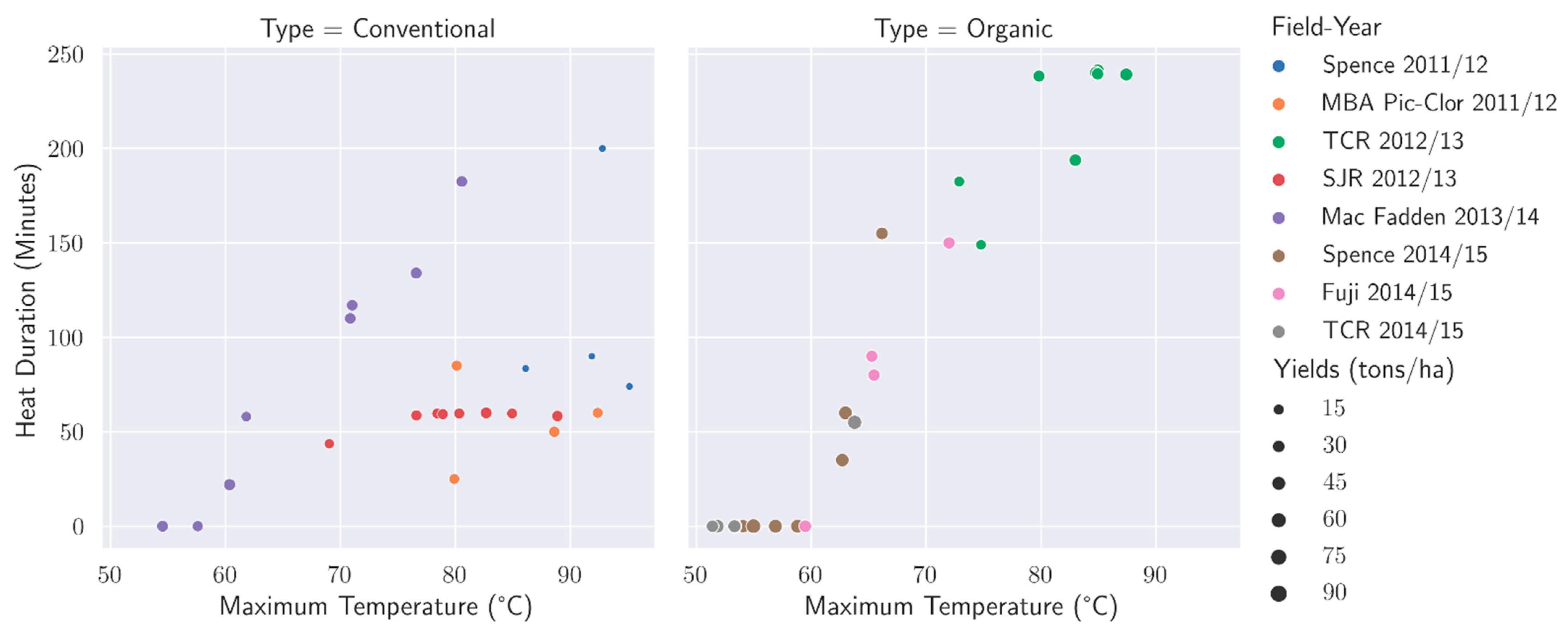
Figure 2 plots trial replicates by production system. Each color corresponds to a particular trial. Each dot represents one replicate. The size of the dot represents the yield for the replicate. Among the conventional trials, replicates in the MacFadden trial showed a wide range in both maximum temperature and heat duration. Other trials tended to show much more variation in one heat variable than in the other. Yields differed across trials more than within trials, as shown by the variations in size of the dots of different colors. Among the organic trials, a significant number of replicates did not achieve a temperature of 60 °C.
Differences in mean values between steam and steam + MSM treatments for both heat variables in conventional trials are significant at the 8% level (p-value ~0.08). The coefficient of variation for heat duration is higher than the coefficient of variation for maximum temperature for all production system–treatment pairs. Table 2 reports summary statistics for heat variables by production system and treatment.

3.1.2. Yield

The primary avenue by which the maximum temperature and heat duration are expected to influence net returns is yield. Treatments in which 60 °C was never achieved tended to have low yields in both conventional and organic trials. Examining the treatment averages, yields were higher for both treatments in the organic trials. Across all replicates, yield had the highest coefficient of variation for steam in a conventional production system (0.47), followed by the two controls (Table 3).

3.1.3. Costs

Table 4 disaggregates average total cost ha−1 into cultural, harvest, and treatment costs. Because costs are averaged across all replicates in all trials for each production system and treatment, and trials differ in their treatments and number of replicates, the cultural cost is not constant across treatments in the organic trials. Cultural cost is a larger share of total costs for the control than for either steam or steam + MSM because there is no treatment cost for the control. Harvest cost increases with yield, so a higher yield reduces the share of treatment cost in total cost. In the conventional trials, the harvest cost accounts for more than half of the total cost for the two treatments: 52% (steam) and 57% (steam + MSM). In the organic trials, harvest cost is around 70% of total costs.

3.1.4. Net Returns

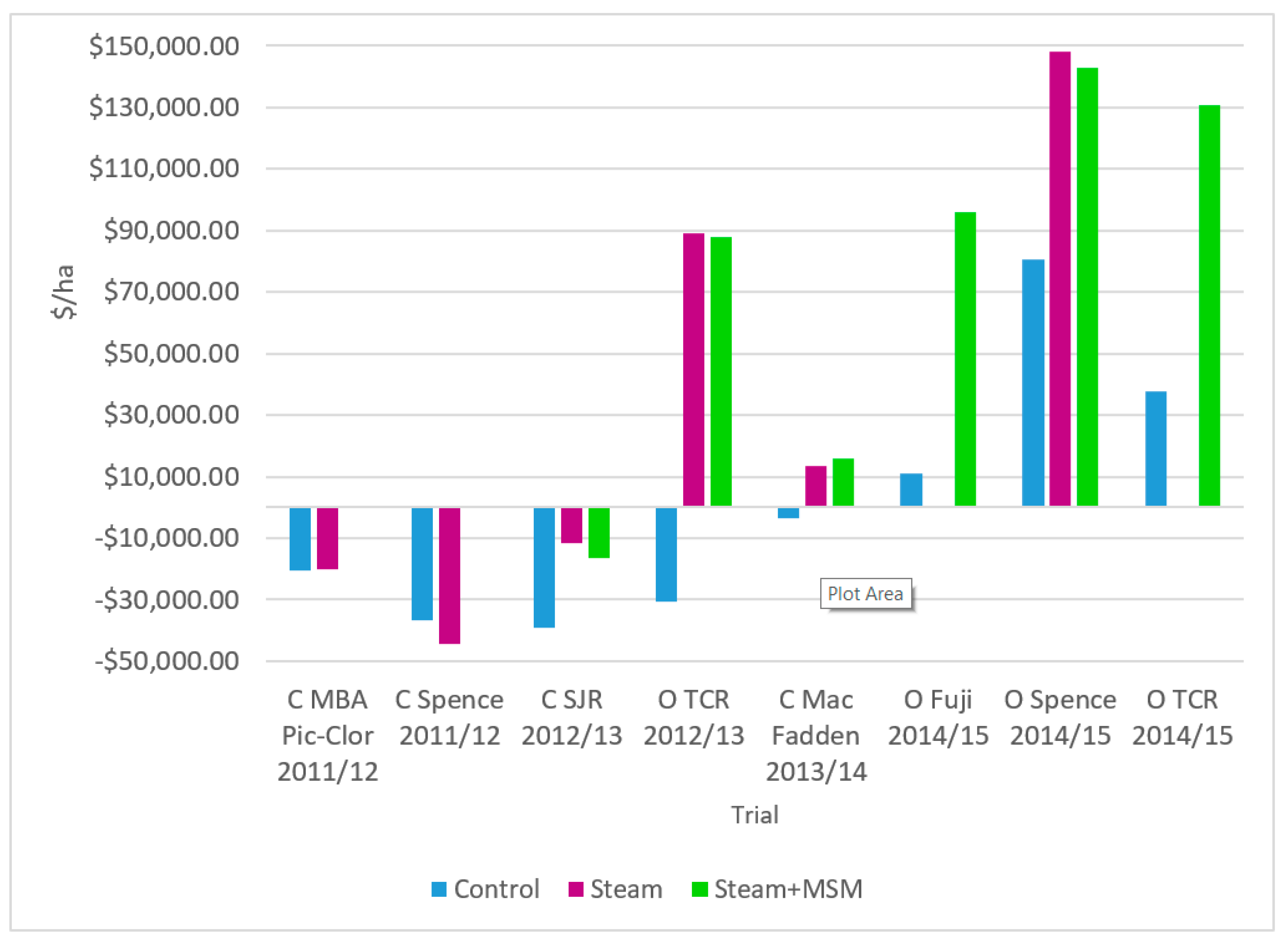
There are significant differences in net returns by trial; differences for a given treatment across trials are mostly larger than differences across treatments for a given trial. The differences across trials by treatment are illustrated in Figure 3, which plots net returns (USD ha−1) by trial and treatment chronologically. Trials are labeled by type of production system (O for organic or C for conventional), trial name, and season. Each treatment is plotted in the same color across all trials.
Table 5 reports net returns for all treatments in all trials. Examining the results for the conventional production system trials, the control always resulted in negative net returns. In all but one of the trials (Spence 2011/12), its net returns were significantly smaller than those for steam and steam + MSM treatments. In conventional production systems, steam had smaller net losses than steam + MSM in one trial (SJR 2012/13), while in the other trial with both treatments (MacFadden 2013/14), it had lower net return gains. The difference was not significant in either. In the organic trials, steam had slightly higher net returns than steam + MSM in the two trials that included both treatments, although neither difference was significant. Both treatments always had significantly higher net returns than the control.

3.2. ANOVA

There were statistically significant differences (a p-value of at least 0.01) for the trial (primary) and treatment (secondary) factors in both the organic and conventional subsamples. Net returns of the two treatments were larger than those of the untreated control, and the difference was statistically significant in both production systems. For organic production, steam and steam + MSM had equal net returns. For conventional production, steam with MSM had net returns higher than steam (p < 0.001), which in turn had higher net returns than the control (p = 0.002) (Table 6).

3.3. Linear Regression

The ANOVA results indicate that steam and steam + MSM result in statistically comparable net returns in organic production systems, while in conventional systems steam + MSM has higher net returns than steam. Given this, we examine these relationships in a structural model using multivariate regression to evaluate the relative magnitudes of the effects of the treatments compared to differences across trials.
As Table 7 reports, regressing net returns on treatment and trial dummies for the organic trials shows that steam and steam + MSM have statistically significant, positive effects on net returns (p < 0.00). All of the field trials have highly statistically significant differences (p = 0.01 or p < 0.00) from the omitted trial TCR 2013/14, consistent with the results of the ANOVA analysis. Notably, coefficients for the two treatments are larger in magnitude than the coefficients for the trials. The magnitude coefficient on the TCR 2012/13 trial, which is the largest trial coefficient, is slightly less than two-thirds of the smaller treatment coefficient (steam + MSM). In spite of the differences in net returns by trial plotted in Figure 3, the treatments have a greater influence.
In the regression analysis for conventional trials, both treatments had positive and significant effects on net returns. All trials had a highly statistically significant difference from the omitted trial (Spence 2011/12). However, unlike the organic analysis, the field trial coefficients were mostly larger than the treatment coefficients. The coefficient for the steam + MSM treatment was smaller than three of the four trial coefficients, and the coefficient for the steam treatment variable was smaller than all four (Table 8). This is consistent with the dramatic differences in net returns across trials plotted in Figure 3.

3.4. Predicting Net Returns as a Function of Maximum Temperature and Heat Duration

The prior analyses demonstrate that pre-plant soil disinfestation with steam increases net returns relative to an untreated control. In this section, we focus on predicting the relationships between net returns and the heat variables.

3.4.1. Single Variable Analysis

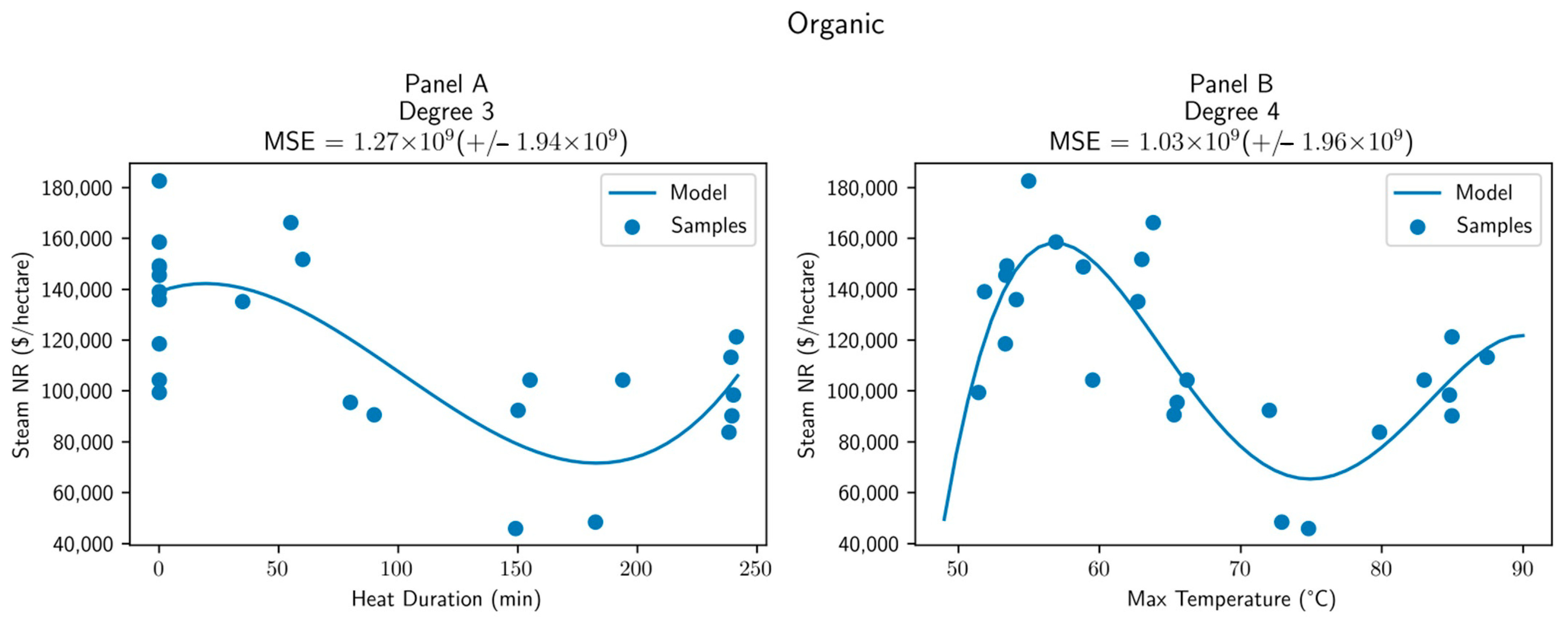
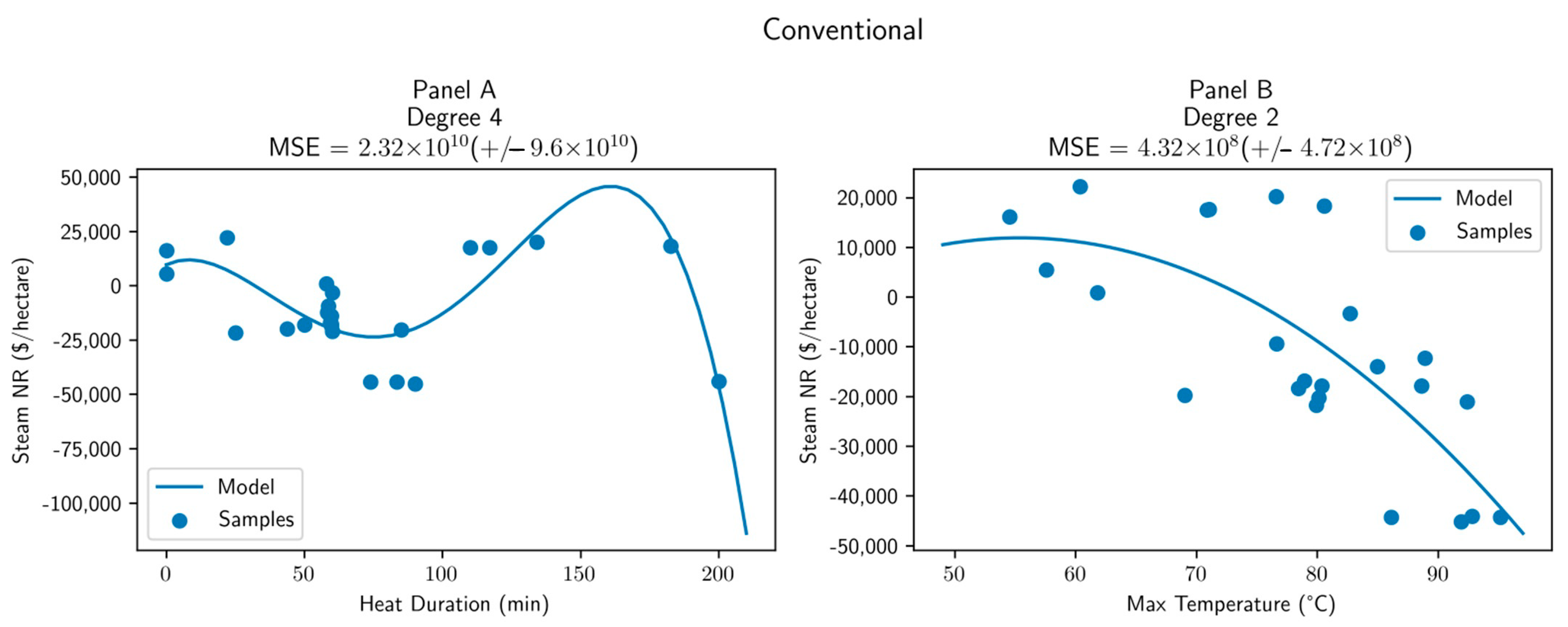
Figure 3 and Figure 4 present the best-fitting models for explaining net returns as a function of heat duration and maximum temperature for organic and conventional trials, respectively. In each panel of the two figures, a blue dot denotes each observation and the line plots the best-fitting model. The heat variable is on the horizontal axis and net returns is on the vertical axis.
For organic production, the best fit for heat duration is the third-degree polynomial (Figure 4A). The large number of replicates with zero heat duration plays a significant role in determining the polynomial, as does the somewhat smaller number of replicates with very long durations. That is, observations are clustered at the two ends of the distribution of observed heat duration. For maximum temperature, the fourth-degree polynomial is the best fit (Figure 4B). There is no clear relationship between the maximum temperature and net returns. The steam-induced temperature rise in soil depends on a multitude of chemical, physical, and technical factors [28,29]. The large number of observations that did not reach 60 °C (leading to zero heat duration) had relatively high net returns. The predicted net returns then decline until a maximum temperature of around 75 °C, at which point they begin to increase again.
For conventional production, the best fit for heat duration is the fourth-degree polynomial (Figure 5A). In the range that accounts for most observations, net returns first decrease then increase with heat duration, suggesting no clear relationship. For maximum temperature, the second-degree polynomial appears to be the best fit (Figure 5B). Net returns decline at an increasing rate as maximum temperature increases.

3.4.2. Joint Analysis

Comparing the average mean square errors, the quadratic model is the best fit for predicting net returns for both organic and conventional production when both heat variables are included (Table 9).
The estimated best-fitting models are:
O r g a n i c N e t R e t u r n s = 23,820 + 583.3 M T 378.4 H D + 0.56 M T 2 + 1.25 M T H D + 0.48 H D 2     C o n v e n t i o n a l N e t R e t u r n s = 87,200 2576.2 M T + 1008.8 H D + 19.3 M T 2 16.4 M T H D + 1.8 H D 2  
Figure 6 plots the iso-net returns curves for each production system using the above equations. In each panel observed maximum temperature–heat duration pairs are indicated by a blue dot. The iso-net returns curves plot all maximum temperature–heat duration pairs that result in the net returns on the label for each curve.
The relationship between the heat variables and net returns varies by production system. For organic strawberries (left-hand panel), a higher maximum temperature increases net returns, as shown by net returns increasing as one moves right, while heat duration decreases net returns, as shown by it decreasing as one moves up. Net returns for organic strawberries are positive. The values for individual replicates range from 46,095 USD ha−1 to 182,584 USD ha−1. The replicate with 73,921 USD ha−1 in net returns achieves a maximum temperature of 55 °C, so its value on the x-axis in the figure is difficult to compare to the iso-net return lines. The adjusted R2 is 0.34.
Conventional strawberries display the opposite relationship. A longer heat duration tends to increase net returns and higher maximum temperature reduces net returns. Across all conventional replicates, the minimum net returns are −45,131 USD ha−1 and the maximum net returns are 22,232 USD ha−1. The iso-net returns line labeled 0 is the set of combinations for which net returns are 0 USD ha−1 for that pair. As one moves left and up from that iso-net return line, net returns increase. The adjusted R2 is 0.74.

3.4.3. Predicting Net Returns by Treatment

Given the high statistical significance of trial dummies in the linear regression models, we used the increment between a replicate’s net returns and the average net returns for the untreated control in its trial as the dependent variable. Results using absolute net returns are reported as Supplementary Materials. Tables reporting MSE for polynomials of degrees 1 to 6 are included as Supplementary Materials.
We first consider steam treatments in organic production systems. A first-order polynomial is the best fit (R2 = 0.62). Figure 7 plots iso-net returns lines and the observed maximum temperature–heat duration pairs. These lines now represent the increment in net returns over the untreated control with the labeled value. Observed pairs are represented by blue dots. Examining those lines, incremental net returns increase with the maximum temperature throughout the observed range; the value of the iso-net returns curves increase as one moves to the right. Heat duration has very little impact, as shown by the nearly vertical iso-net returns curves.
Results are somewhat different for steam + MSM in organic production systems. Here, a quadratic equation is the best fit, with an R2 of 0.41. Examining the observed maximum temperature–heat duration pairs, the increments in net returns are roughly the same for pairs that are low in both dimensions as ones that are high in both dimensions. Net returns are positive in the observed range, although the iso-net returns curves on either side of the observed range are negative (Figure 8).
Moving to the conventional production systems, as in the organic production system, a one-degree polynomial is the best fit for the data on steam treatments (R2 = 0.733), although a two-degree polynomial is a very close second (R2 = 0.729) (the two have the same value if rounded to two digits after the decimal point.) Again, maximum temperature is the primary determinant of the increment in net returns ha−1. In contrast to steam treatments in the organic production system, however, higher maximum temperatures are associated with lower increments in net returns in the conventional system (Figure 9).
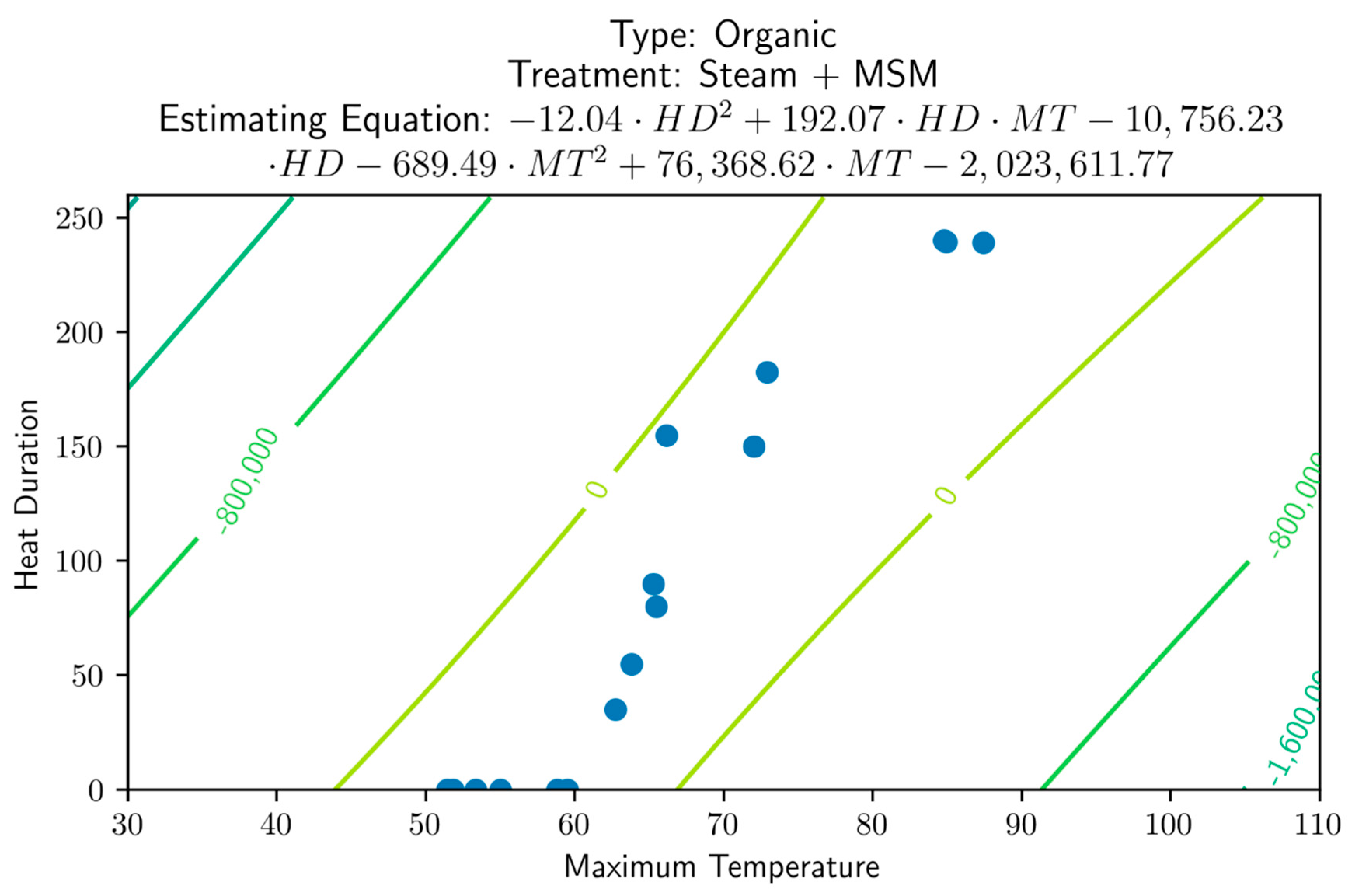
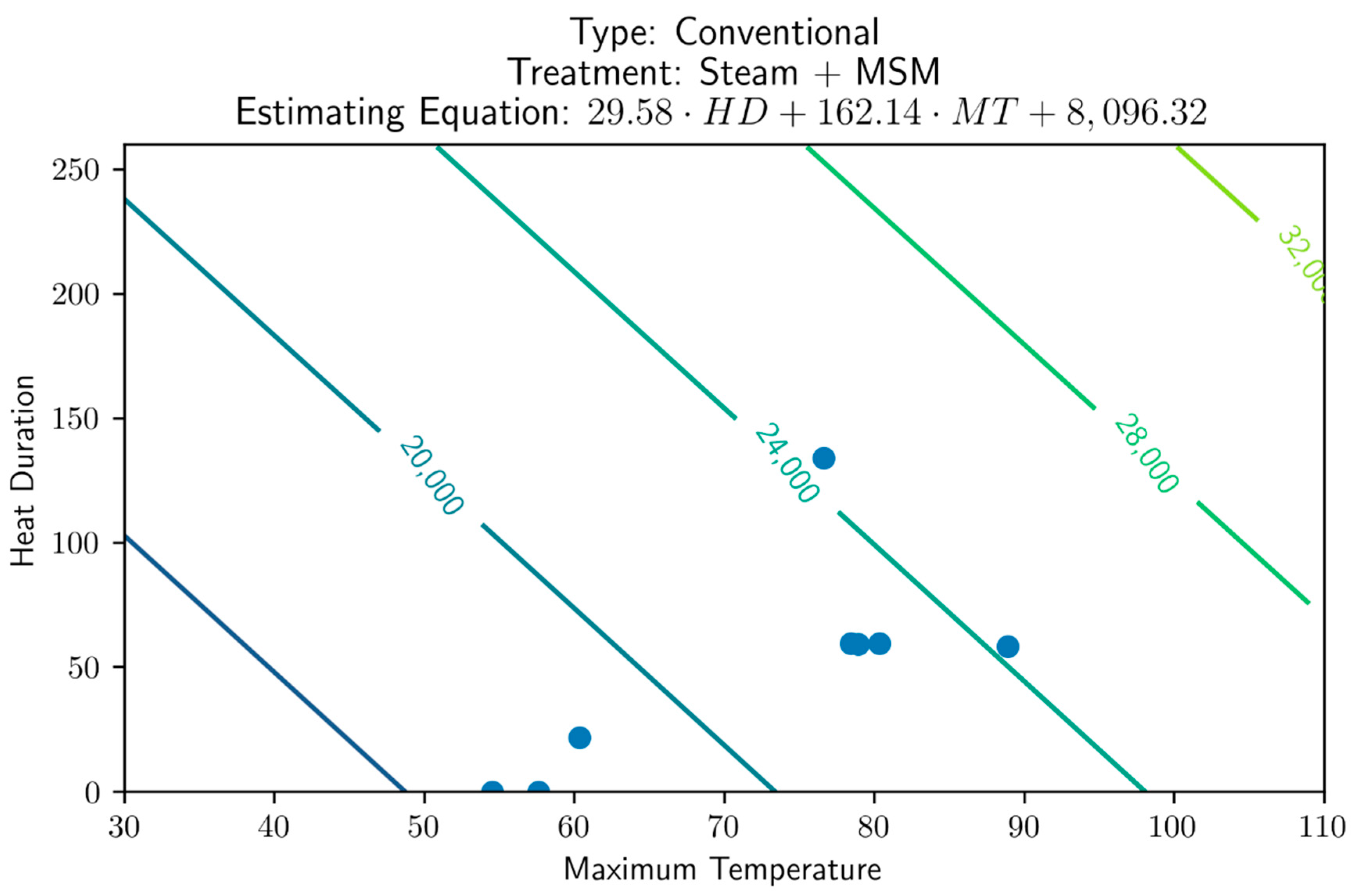
Finally, we consider net returns for steam + MSM treatments in conventional production. A degree-one polynomial is the best fit. Net returns increase with maximum temperature and heat duration; the two are close to perfect substitutes (Figure 10). However, the polynomial’s R2 is −1.09. The negative R2 means that the model does not predict each observation as well as the sample average of net returns does.

3.4.4. Net Returns at Mean Maximum Temperature and Heat Duration

As reported earlier, the mean maximum temperature and heat duration vary by treatment, particularly for treatments in conventional production systems. Using the models derived in the previous subsection, we compare net returns between each treatment and the untreated control. Net returns to the organic treatments are much higher than those for the conventional treatments (Table 10), which is consistent with Figure 2. Steam has higher net returns than steam + MSM, and both have higher net returns than the untreated control in organic production. Steam + MSM and the control have higher net returns than steam in conventional production.
The final column of Table 10 sums these differences and the net returns to the untreated control averaged over the entire dataset. Both treatments and the control for conventional production systems have negative net returns.

3.4.5. Net Return-Maximizing Maximum Temperature and Heat Duration

We calculate the net return-maximizing values of the heat variables for the two sets of data for which a quadratic equation was the best fit: all organic observations using either steam or steam + MSM, and organic observations using steam + MSM. The optimal values are close for the two sets of data, and suggest that a maximum soil temperature slightly above 60 °C achieved for 40–45 min maximizes net returns. For all organic observations, the net return-maximizing maximum temperature is 63 °C, and the net return-maximizing heat duration is 41 min. The resulting increment compared to the untreated control in the same trial is 80,396 USD ha−1. For organic steam + MSM treatments, the corresponding maximum temperature is 62 °C and the corresponding heat duration is 44 min, leading to an increment of 88,396 USD ha−1. These heat durations are noticeably shorter than those conducted in the field trials (Table 2), indicating that the value of increasing heat duration was negative.
While the linear model is the best fit, the quadratic model fits nearly as well for two datasets. For all conventional observations, the R2 of the quadratic model is 0.70, compared to the 0.71 R2 of the linear model. For the conventional steam only observations, the R2 of the quadratic model is 0.729, compared to the 0.734 R2 of the linear model. The two round to the same value when considering only two digits to the right of the decimal point. Given the closeness in fit, we also compute the optimal maximum temperature and heat duration for these models. For all conventional observations, the optimal maximum temperature is 69 °C with an optimal heat duration of 84 min, resulting in a net return increment of 20,916 USD ha−1 over the net returns to the control. For conventional steam only observations, the optimal maximum temperature is substantially higher at 76 °C, and the optimal maximum heat duration is much shorter at only 23 min. The difference in net returns was 17,337 USD ha−1 more than the control.

4. Discussion

Overall, the findings here suggest that steam or steam + MSM may be economically viable in some cases, and that it is not apparent which of the two treatments results in higher net returns. This is consistent with findings in the previous literature discussed in Section 1.1. In terms of economic viability, [8] found that steam or steam plus solarization performed less well than solarization, although steam alone performed better than the untreated control. In terms of relative performance, [15] found in one trial that the steam + MSM treatment performed better than the steam treatment. The ranking was reversed in the other trial.
Gross revenues are a function of yield and price. There are two important considerations regarding the role of price for our analysis. First, if strawberry prices are low, then the revenue from any given yield declines, making it more difficult to cover treatment costs. Second, because organic strawberries obtain a price premium relative to conventional strawberries, an identical yield increase increases organic gross revenues more than conventional gross revenues. In this analysis, organic yields were higher, which amplified the effect of the price premium on net returns.
A primary hypothesis for this analysis was that net returns to steam and steam + MSM treatments will depend on heat duration (the time for which the soil is at a temperature of 60 °C or higher) and the maximum temperature achieved (°C). One of the interesting differences in the results for conventional and organic systems is that when steam and steam + MSM treatments were aggregated, heat duration had a positive effect on net returns, and maximum temperature had a negative effect for organic production, while the signs were reversed in conventional production. Consequently, the optimal maximum temperature was substantially higher, and the optimal heat duration was substantially lower, for the conventional steam only treatment than for the quadratic models in organic systems examined above. This difference is consistent with the differences in achieved maximum temperature and heat duration across sites and treatments.
While the main conclusion from the analysis of the conventional trials was that the data must be augmented with the results of additional trials, the analysis of the organic trials provided several insights. The results for all organic and organic steam + MSM trials suggested that, on average, the net return-maximizing estimated maximum temperatures were slightly higher, and the estimated heat durations much shorter, than the average values realized in the trials. They also suggest that the 60 °C standard for heat duration is close to the optimal maximum temperature. This in turn implies that there is value to achieving roughly that temperature for the time duration necessary for efficacy. This could potentially provide an application standard for commercial growers.
However, any such standard must take additional factors into account. Field-scale steaming is a new method of steam disinfestation, and more research and development is required for more efficient operation, such as balancing fuel requirements with the minimum heat inputs need to kill pathogens. Disease pressure likely plays a role, although further investigation of this hypothesis is required. A next step for researchers could be to investigate the roles of soil type, soil moisture, and other factors on the performance of steam soil disinfestation applications in strawberry production.

5. Conclusions

This study investigated whether the application of steam with or without MSM is an economically sustainable pre-plant soil disinfestation technique for organic and conventional strawberry production in California’s Central Coast region. It found statistically significant differences in net revenues by treatment and trial. For organic production, net returns were statistically similar for the steam and steam + MSM treatments. For conventional production, the steam + MSM treatment had significantly higher net returns than the steam treatment. Predictive polynomial models identified relationships between net returns and two treatment characteristics: maximum temperature (°C) and heat duration (minutes at ≥60 °C). Cross-validated polynomial models outperformed the sample mean for prediction of net returns for five of six subsets of data disaggregated by production system, and by individual treatments or grouping steam and steam + MSM treatments together. Results from two of three organic models suggest that maximum soil temperatures of 62–63 °C achieved for 41–44 min maximizes net returns and may be a basis for further experiments.
This analysis demonstrated the value of using predictive analysis to extract additional information from field trial results. Even with low sample sizes, there are methods available to account for data limitations in order to reduce the chances of overfitting. Evaluating all replicates for all trials, the standard deviations of maximum temperature were similar for the organic and conventional production systems. However, the standard deviations of heat duration for the organic replicates were much larger than those for the conventional ones, increasing the organic models’ predictive power. The difference in the findings for treatments in organic and conventional production systems illustrates the value of beginning with a wide range of values in order to improve the range for which the data enable the estimation of predictive models. This stands in stark contrast to the difficulty of identifying general lessons from a set of field trials with very heterogeneous outcomes.

Supplementary Materials

The following are available online at https://www.mdpi.com/2073-4395/11/1/149/s1, Table S1: Mean Squared Error (MSE) for Fitting of Increment in Net Returns (USD ha−1): Organic, Steam; Table S2: Mean Squared Error (MSE) for Fitting of Increment in Net Returns (USD ha−1): Organic, Steam + MSM; Table S3: Mean Squared Error (MSE) for Fitting of Increment in Net Returns (USD ha−1): Conventional, Steam; Table S4: Mean Squared Error (MSE) for Fitting of Increment in Net Returns (USD ha−1): Conventional, Steam + MSM; Table S5: Mean Squared Error (MSE) for Fitting of Absolute Net Returns (USD ha−1): Organic, Steam; Figure S1: Iso-net return curves for absolute net returns (USD ha−1): organic, steam; Table S6: Mean Squared Error (MSE) for Fitting of Absolute Net Returns (USD ha−1): Organic, Steam + MSM; Figure S2: Iso-net return curves for absolute net returns (USD ha−1): organic, steam + MSM; Table S7: Mean Squared Error (MSE) for Fitting of Absolute Net Returns (USD ha−1): Conventional, Steam; Figure S3: Iso-net return curves for absolute net returns (USD ha−1): conventional, steam; Table S8: Mean Squared Error (MSE) for Fitting of Absolute Net Returns (USD ha−1): Conventional, Steam + MSM; Figure S4. Iso-net return curves for absolute net returns (USD ha−1): conventional, steam + MSM.

Author Contributions

Conceptualization: R.E.G., S.A.F. and M.H.; methodology: A.M. and R.E.G.; software: A.M.; validation: S.A.F., R.E.G., M.H. and A.M.; formal analysis: A.M. and R.E.G.; investigation: S.A.F., R.E.G. and M.H.; resources: S.A.F. and R.E.G.; data curation: A.M. and M.H.; writing—original draft preparation: A.M. and R.E.G.; writing—review and editing: R.E.G., M.H. and S.A.F.; visualization: A.M. and R.E.G.; supervision: R.E.G.; project administration: R.E.G.; funding acquisition: S.A.F. and R.E.G. All authors have read and agreed to the published version of the manuscript.

Funding

USDA NIFA Methyl Bromide Transitions grant 2010-51102-21648 and funding from the California Strawberry Commission, the Propane Education and Research Council, and the Giannini Foundation of Agricultural Economics.

Institutional Review Board Statement

Not applicable.

Informed Consent Statement

Not applicable.

Data Availability Statement

Data sharing not applicable. No new data were created or analyzed in this study. Data sharing is not applicable to this article.

Acknowledgments

Thanks to Driscoll’s Associates and Reiter Affiliated Companies for their support of this research. Thanks especially to Nathan Dorn for operating the steam applicator during several years of testing.

Conflicts of Interest

The authors declare no conflict of interest.

References

  1. Xu, Y.; Goodhue, R.; Chalfant, J.; Miller, T.; Fennimore, S. Economic viability of steam as an alternative to pre-plant soil fumigation in California strawberry production. HortScience 2017, 52, 401–407. [Google Scholar] [CrossRef]
  2. Bolda, M.P.; Tourte, L.; Klonsky, K.M.; De Moura, R.L.; Tumber, K.P. Sample Costs to Produce Organic Strawberries, Central Coast. 2014. Available online: https://coststudyfiles.ucdavis.edu/uploads/cs_public/94/4b/944b5aad-6660-4dcd-a449-d26361afcae2/strawberry-cc-organic-2014.pdf (accessed on 6 January 2021).
  3. Subbarao, K.V.; Kabir, Z.; Martin, F.N.; Koike, S.T. Management of soilborne diseases in strawberry using vegetable rotations. Plant Dis. 2007, 91, 964–972. [Google Scholar] [CrossRef] [PubMed] [Green Version]
  4. Koike, S.T. Crown Rot of Strawberry Caused by Macrophomina phaseolina in California. Plant Dis. 2008, 92, 1253. [Google Scholar] [CrossRef] [PubMed]
  5. Kim, D.S.; Hoffmann, M.; Kim, S.; Scholler, B.A.; Fennimore, S.A. Integration of steam with allyl-isothiocyanate for soil disinfestation. HortScience 2020, 1–6, in preparation. [Google Scholar]
  6. Senner, A.H. Application of Steam in the Sterilization of Soils; US Department of Agriculture: Washington, DC, USA, 1934; 20p.
  7. Shennan, C.; Muramoto, J.; Koike, S.; Baird, G.; Fennimore, S.; Samtani, J.; Bolda, M.; Dara, S.; Daugovish, O.; Lazarovits, G.; et al. Anaerobic soil disinfestation is an alternative to soil fumigation for control of some soilborne pathogens in strawberry production. Plant Pathol. 2018, 67, 51–66. [Google Scholar] [CrossRef]
  8. Muramoto, J.; Gliessman, S.R.; Koike, S.T.; Shennan, C.; Bull, C.T.; Klonsky, K.; Swezey, S. Integrated biological and cultural practices can reduce crop rotation period of organic strawberries. Agroecol. Sustain. Food Syst. 2014, 38, 603–631. [Google Scholar] [CrossRef] [Green Version]
  9. Fennimore, S.A.; Goodhue, R.E. Soil disinfestation with steam: A review of economics, engineering and soil pest control in California strawberry. Int. J. Fruit Sci. 2016, 16, 71–83. [Google Scholar] [CrossRef]
  10. Fennimore, S.A.; Serohijos, R.; Samtani, J.B.; Ajwa, H.A.; Subbarao, K.V.; Martin, F.N.; Daugovish, O.; Legard, D.; Browne, G.T.; Muramoto, J.; et al. TIF film, substrates and nonfumigant soil disinfestation maintain fruit yields. Calif. Agric. 2013, 67, 139–146. [Google Scholar] [CrossRef] [Green Version]
  11. Miller, T.C.; Samtani, J.B.; Fennimore, S.A. Mixing steam with soil increases heating rate compared to steam applied to still soil. Crop. Prot. 2014, 64, 47–50. [Google Scholar] [CrossRef]
  12. Dabbene, F.; Gay, P.; Tortia, C. Modelling and control of steam soil disinfestation processes. Biosyst. Eng. 2003, 84, 247–256. [Google Scholar] [CrossRef]
  13. Gay, P.; Piccarolo, P.; Aimonino, D.R.; Tortia, C. A high efficiency steam soil disinfestation system, part I: Physical background and steam supply optimisation. Biosyst. Eng. 2010, 107, 74–85. [Google Scholar] [CrossRef]
  14. Wei, H.; Goodhue, R.; Muramoto, J.; Sumner, D. Economic Statistics of California’s Organic Agriculture: 2013–2016; University of California Agricultural Issues Center: Davis, CA, USA, 2020; Available online: https://aic.ucdavis.edu/wp-content/uploads/2020/10/CA-Organic-Ag-13-16.pdf (accessed on 6 January 2021).
  15. Shennan, C.; Muramoto, J. Design and Management of Organic Strawberry/Vegetable Rotations. Ob-Tenido de CAL-CORE. 11 April 2016. Available online: https://calcorenetwork.sites.ucsc.edu/2016/04/03/design-and-management-of-organic-strawberryvegetable-rotations/ (accessed on 6 January 2021).
  16. McQueen, R.J.; Garner, S.R.; Nevill-Manning, C.G.; Witten, I.H. Applying machine learning to agricultural data. Comput. Electron. Agric. 1995, 12, 275–293. [Google Scholar] [CrossRef] [Green Version]
  17. Hoffmann, M.; Ajwa, H.A.; Westerdahl, B.B.; Koike, S.T.; Stanghellini, M.; Wilen, C.; Fennimore, S.A. Multi-tactic pre-plant soil fumigation with allyl isothiocyanate in cut-flower and strawberry. HortTechnology 2020. in print. [Google Scholar] [CrossRef]
  18. Michuda, A.; Goodhue, R.E.; Klonsky, K.; Baird, G.; Toyama, L.; Zavatta, M.; Muramoto, J.; Shennan, C. The economic viability of suppressive crop rotations for the control of verticillium wilt in organic strawberry production. Agroecol. Sustain. Food Syst. 2018, 43, 984–1008. [Google Scholar] [CrossRef]
  19. Hoffmann, M.; Barbella, A.; Miller, T.; Broome, J.; Martin, F.; Koike, S.; Rachuy, J.; Greene, I.; Dorn, N.; Goodhue, R.; et al. Weed and pathogen control with steam in California strawberry production. Acta Hortic. 2016, 1156, 593–602. [Google Scholar] [CrossRef]
  20. Liakos, K.G.; Busato, P.; Moshou, D.; Pearson, S.; Bochtis, D. Machine learning in agriculture: A review. Sensors 2018, 18, 2674. [Google Scholar] [CrossRef] [PubMed] [Green Version]
  21. Fennimore, S.A.; Martin, F.N.; Miller, T.C.; Broome, J.C.; Dorn, N.; Greene, I. Evaluation of a mobile steam applicator for soil disinfestation in California strawberry. HortScience 2014, 49, 1542–1549. [Google Scholar] [CrossRef]
  22. Lachenbruch, P.A.; Mickey, M.R. Estimation of error rates in discriminant analysis. Technometrics 1968, 10, 1–11. [Google Scholar] [CrossRef]
  23. Koike, S.T.; Kirkpatrick, S.C.; Gordon, T.R. Fusarium Wilt of Strawberry Caused by Fusarium oxysporum in California. Plant Dis. 2009, 93, 1077. [Google Scholar] [CrossRef]
  24. Daugovish, O.; Howell, A.; Fennimore, S.; Koike, S.; Gordon, T.; Subbarao, K. Non-fumigant treatments and their combinations affect soil pathogens and strawberry performance in southern California. Int. J. Fruit Sci. 2016, 16 (Suppl. S1), 37–46. [Google Scholar] [CrossRef]
  25. Atwood, D.; Paisley-Jones, C. Pesticides Industry Sales and Usages 2008–2012 Market Estimates; Office Pesticide Programs, Office Chem. Safety Poll. Prev., U.S. Environ. Protection Agency: Washington, DC, USA, 2017.
  26. Bolda, M.P.; Tourte, L.; Murdock, J.; Sumner, D.A. Sample Costs to Produce and Harvest Strawberries, Central Coast Region. 2016. Available online: https://coststudyfiles.ucdavis.edu/uploads/cs_public/e7/6d/e76dceb8-f0f5-4b60-bcb8-76b88d57e272/strawberrycentralcoast-2016-final2-5-1-2017.pdf (accessed on 6 January 2021).
  27. Inderbitzin, P.; Ward, J.; Barbella, A.; Solares, N.; Izyumin, D.; Burman, P.; Chellemi, D.O.; Subbarao, K.V. Soil microbiomes associated with Verticillium wilt-suppressive broccoli and chitin amendments are enriched with potential bio-control agents. Phytopathology 2018, 108, 31–43. [Google Scholar] [CrossRef] [PubMed] [Green Version]
  28. Samtani, J.B.; Gilbert, C.; Weber, J.B.; Subbarao, K.V.; Goodhue, R.E.; Fennimore, S.A. Effect of steam and solarization treatments on pest control, strawberry yield, and economic returns relative to methyl bromide fumigation. HortScience 2012, 47, 64–70. [Google Scholar] [CrossRef] [Green Version]
  29. California Department of Food and Agriculture. California Agricultural Statistics Review, 2018–2019; California Department of Food and Agriculture: Sacramento, CA, USA, 2019. Available online: https://www.cdfa.ca.gov/statistics/PDFs/2018-2019AgReportnass.pdf (accessed on 6 January 2021).
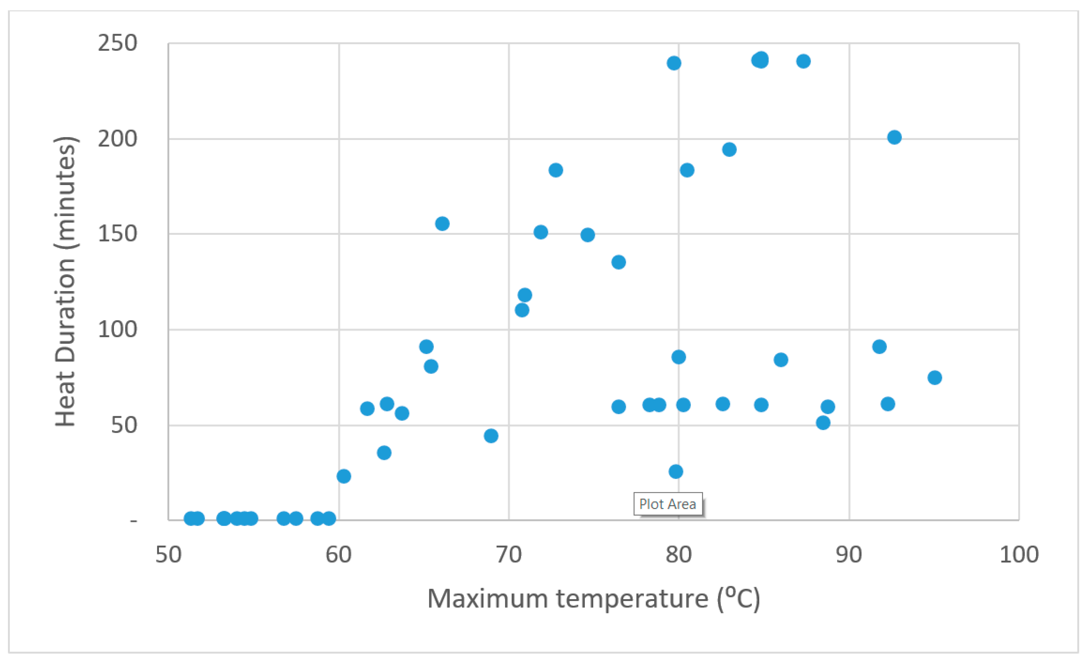
Figure 1. Maximum temperature (°C) and heat duration (minutes) pairs: all steam and steam + MSM treatments. Each dot represents the maximum temperature and heat duration for a single trial replicate.
Agronomy 11 00149 g001
Figure 2. Maximum temperature (°C) and heat duration (minutes) pairs by production system. Each dot represents the maximum temperature and heat duration for a single trial replicate. Replicates in each trial are a different color. The size of each dot corresponds to the yields achieved by that replicate.
Agronomy 11 00149 g002
Figure 3. Net returns (USD ha−1) by treatment and trial, ordered chronologically. O = organic, C = conventional. Each treatment is assigned a specific color across all trials: the control is blue, steam is magenta, and steam + MSM is green. Not all trials included all treatments.
Agronomy 11 00149 g003
Figure 4. Polynomials by degree for organic system: individual heat variables. (A) shows the optimal fitted model for predicting net returns (USD ha−1) as a function of heat duration (minutes) (adjusted R2 = 0.54). (B) shows the optimal fitted model for predicting net returns as a function of maximum temperature (°C) (adjusted R2 = 0.67). In each panel the blue dots indicate observations, and the line plots the fitted model. All steam and steam + MSM replicates included.
Agronomy 11 00149 g004
Figure 5. Polynomials by degree for conventional system: individual heat variables. Panel (A) shows the optimal fitted model for predicting net returns (USD ha−1) as a function of heat duration (minutes) (adjusted R2 = 0.61). (B) shows the optimal fitted model for predicting net returns as a function of maximum temperature (°C) (adjusted R2 = 0.57). In each panel the blue dots indicate observations, and the line plots the fitted model. All steam and steam + MSM replicates included.
Agronomy 11 00149 g005
Figure 6. Iso-net returns curves for organic (A) and conventional (B) strawberries. Each line is the set of points that results in net returns (USD ha−1) with the labeled value. Blue dots plot observed maximum temperature (°C)–heat duration (minutes) pairs. All steam and steam + MSM replicates included. R2 = 0.34 (organic) and R2 = 0.74 (conventional).
Agronomy 11 00149 g006
Figure 7. Iso-net returns curves for the increment in net returns (USD ha−1) relative to the untreated control: organic, steam. Each line is the set of points that results in an increment in net returns with the labeled value. Blue dots plot observed maximum temperature (°C)–heat duration (minutes) pairs. The equation above the figure reports the estimated coefficients. R2 = 0.62.
Agronomy 11 00149 g007
Figure 8. Iso-net returns curves for the increment in net returns (USD ha−1) relative to the untreated control: organic, steam + MSM. Each line is the set of points that results in an increment in net returns with the labeled value. Blue dots plot observed maximum temperature (°C)–heat duration (minutes) pairs. The equation above the figure reports the estimated coefficients. R2 = 0.41.
Agronomy 11 00149 g008
Figure 9. Iso-net returns curves for the increment in net returns (USD ha−1) relative to the untreated control: conventional, steam only. Each line is the set of points that results in an increment in net returns with the labeled value. Blue dots plot observed maximum temperature (°C)–heat duration (minutes) pairs. The equation above the figure reports the estimated coefficients. R2 = 0.73.
Agronomy 11 00149 g009
Figure 10. Iso-net returns curves for the increment in net returns (USD ha−1) relative to the untreated control: conventional, steam only. Each line is the set of points that results in an increment in net returns with the labeled value. Blue dots plot observed maximum temperature (°C)–heat duration (minutes) pairs. The equation above the figure reports the estimated coefficients. R2 = −1.09.
Agronomy 11 00149 g010
Table 1. Summary of trials. Includes season, production system, which treatments were included, and the rate of the mustard seed meal (MSM) amendment.
Trial (Season)Production SystemSteam IncludedSteam + MSM Included (MSM Rate)
MBA (2011/12)ConventionalYesNo
Spence (2011/12)ConventionalYesNo
SJR (2012/13)ConventionalYesYes (3368 kg ha−1 pelletized MSM)
TCR (2012/13)OrganicYesYes (3368 kg ha−1 pelletized MSM)
MacFadden (2013/14)ConventionalYesYes (3368 kg ha−1 pelletized MSM)
Fuji (2014/15)OrganicNoYes (2245 kg ha−1 pelletized MSM)
Spence (2014/15)OrganicYesYes (2245 kg ha−1 pelletized MSM)
TCR (2014/15)OrganicNoYes (2245 kg ha−1 pelletized MSM)
Table 2. Maximum temperature (°C) and heat duration (minutes) by treatment and production system. Includes mean and standard deviation and the total number of replicates across all trials used to calculate the descriptive statistics.
TreatmentReplicatesMaximum Temperature (°C)Heat Duration
(Minutes)
MeanStandard DeviationMeanStandard Deviation
Conventional
Steam1681.59.784.847.9
Steam + MSM871.912.649.143.4
Organic
Steam967.013.598.1107.2
Steam + MSM1666.011.791.695.4
Table 3. Yield (t ha−1) by treatment and production system. Includes number of trials, total number of replicates from those trials, mean, standard deviation, and coefficient of variation.
TreatmentTrialsReplicatesMeanStandard DeviationCoefficient of Variation
Conventional
Control42427.011.00.4
Steam41633.116.00.47
Steam + MSM2844.96.10.13
Organic
Control42544.614.80.32
Steam2970.414.40.19
Steam + MSM41668.813.00.18
Table 4. Disaggregated cost (USD ha−1) by production system and treatment. The share of total cost is included in parentheses.
Production SystemConventionalOrganic
Cultural CostHarvest CostTreatment CostCultural CostHarvest CostTreatment Cost
Treatment
Control37,472 (0.38)60,069 (0.62)0
(0.00)
38,468 (0.23)126,191 (0.77)0
(0.00)
Steam37,472 (0.36)53,708 (0.52)12,355
(0.12)
38,484 (0.22)127,990 (0.72)12,355
(0.07)
Steam + MSM37,472 (0.29)72,792 (0.57)17,139
(0.13)
38,459 (0.21)125,178 (0.69)17,139
(0.09)
Table 5. Net returns (USD ha−1) by treatment and trial. Net returns calculated as gross revenues minus treatment costs and cultivation costs.
ControlSteamSteam + MSM
Conventional
MacFadden 2013/14−3591 (A)13,630 (B)16,037 (B)
MBA Pic-Clor 2011/12−20,570 (A)−20,179 (B)
SJR 2012/13−39,107 (A)−11,571 (B)−16,303 (B)
Spence 2011/12−36,827 (A)−44,433 (A)
Organic
Fuji 2014/1511,174 (A) 95,803 (B)
Spence 2014/1580,554 (A)148,256 (B)142,806 (B)
TCR 2012/13−30,667 (A)88,909 (B)87,714 (B)
TCR 2014/1537,804 (A) 130,872 (B)
Note: Treatments with the same letter within each field trial are not significantly different.
Table 6. Split-plot ANOVA: strawberry net returns (USD ha−1) by production system. The trial is the primary factor and the treatment is the secondary factor.
TreatmentNet ReturnsGroups
Organic
Steam121,880A
Steam + MSM114,299A
Control27,023B
Conventional
Steam + MSM−133A
Steam−16,638B
Control−23,799C
Table 7. Net returns (USD ha−1) regressed on treatment and field trial dummies: organic.
CoefficientStandard Errort Statp-Value
Intercept39,71991024.367.62 × 10−5
Steam91,36994149.711.67 × 10−12
Steam + MSM89,239761211.723.98 × 10−15
Fuji 2014/15−30,84911,693−2.640.01
Spence 2014/1528,26410,3532.739.08 × 10−3
TCR 2012/13−56,04810,459−5.362.92 × 10−6
Adj. R 2 0.86
DW1.98
JB0.405
Cond. No.6.51
Note: Steam and Steam + MSM coded as indicator variables, where Steam = 1 when treated with steam and 0 otherwise, and Steam + MSM = 1 when treated with steam + MSM and 0 otherwise. Adj. R 2 denotes the adjusted R 2 statistic. DW denotes the Durbin–Watson statistic for autocorrelation in residuals. JB denotes the Jacques–Bera test for normality. Cond. No. denotes the condition number of the moment matrix, a test for multicollinearity.
Table 8. Net returns (USD ha−1) regressed on treatment and field trial dummies: conventional.
CoefficientStandard Errort Statp-Value
Intercept−46,2513548−13.032.36 × 10−16
Steam11,24229813.775.03 × 10−4
Steam + MSM17,50338494.554.55 × 10−5
MacFadden 2013/1444,686408210.947.04 × 10−15
MBA Pic-Clor 2011/1220,25545544.456.25 × 10−5
SJR 2012/1312,54340823.073.72 × 10−3
Adj. R 2 0.81
DW1.02
JB0.90
Cond. No.6.37
Note: Steam and Steam + MSM coded as indicator variables, where Steam = 1 when treated with steam and 0 otherwise, and Steam + MSM = 1 when treated with steam + MSM and 0 otherwise. Adj. R 2 denotes the adjusted R 2 statistic. DW denotes the Durbin–Watson statistic for autocorrelation in residuals. JB denotes the Jacques–Bera test for normality. Cond. No. denotes the condition number of the moment matrix, a test for multicollinearity.
Table 9. Polynomials by degree: predicting net returns (USD ha−1) as a function of heat duration (minutes) and maximum temperature (°C) by production system.
Degree of PolynomialAverage Mean Square Error
OrganicConventional
15.52 × 10⁹ 4.22 × 10⁹
22.53 × 1093.08 × 109
31.02 × 10103.42 × 109
42.82 × 10114.76 × 109
52.69 × 10168.47 × 1011
63.72 × 10162.20 × 1015
Table 10. Increment in net returns (USD ha−1) by treatment at mean maximum temperature (°C) and mean heat duration (minutes).
TreatmentDifference in Net Returns ha−1 *Net Returns ha−1 **
All organic77,393104,404
Organic, steam only90,642117,654
Organic, steam + MSM only88,120115,132
All conventional13,494−10,295
Conventional, steam only9013−14,776
Conventional, steam + MSM21,212−2579
* Computed using trial-level net returns for the untreated control; ** Computed using overall mean net returns for the untreated control.
Publisher’s Note: MDPI stays neutral with regard to jurisdictional claims in published maps and institutional affiliations.