Abstract
Residue decomposition from cattle dung is crucial in the nutrient cycling process in Integrated Crop–Livestock Systems (ICLS). It also involves the impact of the presence of trees exerted on excreta distribution, as well as nutrient cycling. The objectives of this research included (i) mapping the distribution of cattle dung in two ICLS, i.e., with and without trees, CLT and CL, respectively, and (ii) quantification of dry matter decomposition and nutrient release (nitrogen—N, phosphorus—P, potassium—K, and sulphur—S) from cattle dung in both systems. The cattle dung excluded boxes were set out from July 2018 to October 2018 (pasture phase), and retrieved after 1, 7, 14, 21, 28, 56 and 84 days (during the grazing period). The initial concentrations of N (~19 g kg−1), P (~9 g kg−1), K (~16 g kg−1), and S (~8 g kg−1) in the cattle dung showed no differences. The total N, P, K and S released from the cattle dung residues were less in the CLT system (2.2 kg ha−1 of N; 0.7 kg ha−1 of P; 2.2 kg ha−1 of K and 0.6 kg ha−1 of S), compared to the CL (4.2 kg ha−1 of N; 1.4 kg ha−1 of P; 3.6 kg ha−1 of K and 1.1 kg ha−1 of S). Lesser quantities of cattle dung were observed in the CLT (1810) compared to the CL (2652), caused by the lower stocking rate, on average, in this system (721 in the CL vs. 393 kg ha−1 in the CLT) because of the reduced amount of pasture in the CLT systems (−41%), probably due to light reduction (−42%). The density of the excreta was determined using the Thiessen polygon area. The CL system revealed a higher concentration of faeces at locations near the water points, gate and fences. The CLT affects the spatial distribution of the dung, causing uniformity. Therefore, these results strengthen the need to understand the nutrient release patterns from cattle dung to progress fertilisation management.
1. Introduction
Sustainable Intensification (SI) is the process in which agricultural production is expanded or saved while advancing environmental improvements [1]. Among the strategies for the SI of land use, we highlight Integrated Crop–Livestock Systems (ICLS) [2], including agroforestry systems [1], which are linked to the management of the soil conservation practices, such as the no-till system.
ICLS include the development of a diversity of agricultural pursuits in the same area, ensuring several medium- and long-term advantages [3]. Through ICLS, soil fertility and nutrient cycling can be improved, while promoting the sustainable intensification of land, like low fossil energy inputs, diversification of the producer’s income sources, high biodiversity and biomass production, consideration for animal welfare, and rational water use [2,3].
ICLS with trees in pasture locations, in addition to providing shelter and shade, provide greater resilience to the system, as well as better pasture quality [4], as well as enhanced ecosystem services [2]. Trees also promote biodiversity, in an effort to recover nutritional security and global food yield [5]. In ICLS, the integration of trees may contribute to nutrient cycling by absorbing the nutrients present in the subsoil and releasing them into the topsoil [6]. However, in shaded areas, the grasses exhibit physiological and anatomical changes to compensate for the low quantity and quality of light [7], with observable impacts on the nutritive value and production [8]. These differences in the ingested forage, in terms of quantity and quality, may, consequently, alter the composition and quality of the cattle dung. Further, the tree component of the ICLS may influence the decomposition either directly or indirectly through microclimate or the decomposer communities [9,10]. Although cattle dung residues are nutrient-rich and could be valuable organic sources [11,12,13,14,15,16,17,18], little is known about dung decomposition and subsequent nutrient release in ICLS that include trees.
In the open pastures, i.e., systems without trees, the distribution pattern of cattle excreta and, consequently, in which the nutrients are returned to the pasture, is, in general, not homogeneous [13,19]. As a result, crop performance is affected, particularly in ICLS, due an unequal distribution of cattle dung in the previous pasture [20]. For instance, studies showed that in areas with the largest presence of bovine dung in ICLS, the availability of phosphorus (P) and soil potassium (K) increased by 38% and 122%, and, consequently, the presence of these nutrients in the plant increased by 7% and 41%, respectively. These positive results increased the soybean yield by 23%, in areas with presence of dung input in relation to absence [21]. Therefore, this heterogeneous pattern of nutrient distribution from animal excreta and the occurrence of such returns in different areas increases the heterogeneity of nutrient return in the soils [13,20]. Thus, the challenge is to address strategies to improve the spatial distribution of bovine dung production, to avoid the very concentrated occurrence of bovine dung in some attractive points of the field, as observed in the literature [20,21], regardless of the grazing intensity [21].
Seasons can influence animal behaviour and the spatial and temporal distribution of cattle dung. For instance, in the pasture-based dairy system, with evaluation performed during three different periods per year, [20] observed that the concentrations of faeces and urine during three warm-season observations were higher next to the water tank. However, during the winter, the animals reduced their search for water [20]. Further, under tropical conditions, a few authors noted that, in the ICLS with trees (CLT), cattle deposit their faeces and urine in a more uniform distribution pattern [19,22]. This occurs because, in CLT systems, thermal comfort features such as shade and tree trunks (scalers) are well distributed throughout the area [22]. In other words, with such good tree distribution, the tendency is towards a more uniform faeces distribution [19,22]. This occurs because the animals prefer to remain in the shade of trees for all the daytime period, to avoid the high temperatures and solar radiation, especially observed for the animals in tropical zones [23]. However, since the stocking phase in a typical ICLS of South Brazil occurs during the winter, the frequency of animals searching for shade can be reduced, as for water troughs [20]. Therefore, additional studies are necessary to investigate the tree effect on cattle dung distribution at each season.
We hypothesized that, under subtropical conditions, in a typical ICLS of South Brazil (Cfb of Köppen), i.e., with summer crops, like soybean and maize, and cool-season pastures (e.g., ryegrass plus black oat) during the winter, trees may exert a smaller influence on cattle activities (i.e., the animals would reduce their search for shade during the winter, due to a lower heat load in this period) and, consequently, on the dung distribution. Further, the decomposition rate and nutrient release from the cattle dung could be affected by changes in the composition of the residues derived from the association with trees. Understanding of these factors will enable the ICLS managers to better synchronize the nutrient release with nutrient demand in the subsequent crops. The objective of this study was to assess the impact of including trees in the ICLS on the faeces distribution from heifers, during the winter, and, to quantify the dry matter decomposition and nutrient release (N, P, K and S are the most commonly required nutrients in tropical and subtropical agriculture) from these cattle dung residues in two ICLS (with and without eucalyptus trees).
2. Materials and Methods
2.1. Characterization and History of the Experimental Area
A field experiment was conducted at the Agronomic Institute of Paraná, Ponta Grossa, PR (25°07′24.3′′ S, 50°02′58.6′′ W) in Southern Brazil. The local climate is humid subtropical (Cfb according to the Köppen Climate Classification), with frequent occurrence of frost. The mean annual temperature is 18.3 °C, ranging from 9.2 °C in July to 27.6 °C in February, with a mean annual rainfall of 1239 mm (Table 1). The soil is of the Typic Distrudept and Rhodic Hapludox variety [24] with 270, 30 and 710 g kg−1 of clay, silt, and sand, respectively, in the 0–20 cm layer. Chemical analysis of the soil revealed the following results: 4.9 pH (CaCl2); 23.4 mg dm−3 of phosphorus (P; Mehlich–1); 0.2, 2.7 and 1.1 cmolc dm−3 of exchangeable potassium (K), calcium and magnesium, respectively; base saturation of 48.4%; and carbon (Walkley–Black) was 14.9 g dm−3.

Table 1.
Mean minimum–maximum monthly temperature (°C) and total rainfall (mm) during the experimental period (2018) and historical mean (HM).
In 2006, three tree species (silver oak, Grevillea robusta, eucalypt, Eucalyptus dunnii and pink pepper, Schinus mole) were planted in the ICLS (with trees, CLT). The species were interspersed in the same rows, but running crosswise in relation to the slope, maintaining 3 × 14 m spacing (238 trees ha−1); for more details see [25]. During the 2013 summer, the pink pepper trees were removed, as many of them had been damaged by cattle activity [26]. Furthermore, the tree density was reduced by thinning the silver oak in November 2014. Therefore, during the present study, the new tree arrangement was 9 × 28 m (~40 trees ha−1), which comprised only eucalyptus.
During the first three winters, i.e., in 2007, 2008 and 2009, black oat (Avena strigosa) was grown for soil cover, prior to soybean (Glycine max), maize (Zea mays) and sorghum (Sorghum bicolor × Sorghum sudanense) crops, respectively, in the summer, using no tillage. Since the 2010 winter, the production system of integrated cattle grazing (Purunã beef heifers) on the cool-season pastures (ryegrass, Lolium multiflorum plus black oat). During the stocking phase, the pasture was managed in order to maintain a sward height (SH) constant, i.e., at 20 cm, by using continuous stocking and the put-and-take method [27]. Maize or soybean crops were cultivated alternately in the summer, in the same region.
In the current study, the black oat (cv. IPR61) plus annual ryegrass (cv. São Gabriel) mixture was sown at a seeding rate of 45 and 15 kg ha−1, respectively, in May 2018, and 400 kg ha−1 of commercial N–P–K fertiliser 04–30–10 (N–P2O5–K2O) was applied. Urea was applied approximately 30 days after the pasture was sown, at the rate of 90 kg ha−1 (i.e., 18 June 2018).
The experimental area (2.3 ha) was divided into two experimental units (see Figure 1): one experimental unit (1.2 ha) was used in the CLT system and another experimental unit (1.1 ha) in the CL. This experiment has been part of a long-term study protocol. For more details, see [28].
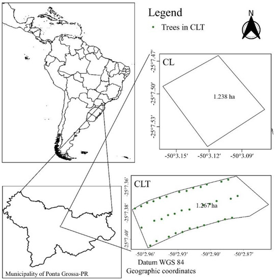
Figure 1.
The experimental site at Ponta Grossa, Paraná, Brazil. CL: crop–livestock only; and CLT: crop–livestock with trees.
The mean percentage of light reduction under the tree canopy in the CLT system compared to that of the CL (treeless) was calculated in May (spring) 2018 and in December (summer) 2018, using two ceptometers (AccuPAR LP–80, Decagon Equipment Co., Pullman, WA). One was positioned under full sunlight, while the other was placed under the trees (Figure 1). Evaluations (one day per month, i.e., 29 May 2018 and 6 Dec. 2018) were done every 30 min, between 9:00 a.m. and 15:00 p.m. The decrease in the photosynthetically active radiation was calculated by the difference between the two values recorded by the ceptometers.
2.2. Experimental Design, Treatments and Performance of the Experiment
The split-plot randomized experimental design was used. The main plots included two types of ICLS systems (with and without trees, CLT and CL, respectively). The subplots were different times (at 1, 7, 14, 21, 28, 56 and 84 days after grazing commenced) and replicated six times.
During the winter (i.e., pasture measurements), the animals employed were Purunã (¼ Charolais, ¼ Caracu, ¼ Canchim, and ¼ Aberdeen Angus) cattle heifers with an age of ~10 months and weighing 216 ± 24 kg in 2018. Stocking season began on 05 July 2018, with grazing commencing at approximately 50 days after sowing, i.e., when all the paddocks reached at least 24 ± 1 cm height, on average. Heifers grazed until 17 October 2018 for a total of 104 grazing days. The short stocking with a variable number of animals periodically adjusted in the CLT in 2018 was caused by a severe drought in July (only 11 mm rainfall) that undermined the grassland productivity. All the animals had unrestricted access to shade in the CLT plots and clean water and mineral supplements throughout the experiments in the CLT and CL plots.
Herbage mass [kg dry matter (DM) ha−1] was estimated at approximately every 21 days, with five cuts at ground level, in each experimental unit, within a quadrat of 0.25 m² (50 × 50 cm). The cuts were made at random inside each experimental unit. The samples were then oven dried (48 h at 60 °C) and weighed. In 2018, the cuts were done once every 21 days.
Animals were weighed every ~21 days (for a total of five stocking periods for 2018) after an approximately 15 h fasting from solids. The stocking rate (SR, kg ha−1, was calculated by adding the average live weight (LW) of the test animals with the average LW of each put-and-take animal, multiplying by the number of days they remained in each experimental unit and dividing by the total number of grazing days during each period. The average daily gain (ADG), expressed in g animal−1 day−1 was calculated as the difference between the final and initial weights of the test animals divided by the number of days in each stocking period. The gain per hectare (Gha), expressed in kg ha−1 was obtained by multiplying the animals ha−1 by the ADG of the test animals and the total number of grazing days.
2.3. Sampling and Chemical Analyses
Nutrient cycling (N, P, K and S) was evaluated from July 2018 up to October 2018, where the decomposition of DM bovine dung residue on N, P, K and S release were evaluated. At the beginning of the grazing period, 36 cattle dung from different experimental units were marked to accompany the natural degradation process and six cattle dung were collected immediately after defaecation by the bovines and carefully transferred into a plastic bag in a thermal box with ice. To avoid any increase in the cattle dung decomposition via physical action, such as animal trampling, grazing exclusion boxes were used. At the time the representative cattle for dung in the ranging area in the experimental units were chosen, the boxes were allocated to protect the cattle dung. The box protected site was maintained without grazing for a period.
Each experimental unit of the CL and CLT systems had 36 cattle dung, during the beginning of the grazing period, for retrieval at 1, 7, 14, 21, 28, 56 and 84 days after grazing commenced. Total dung dry matter contents were oven-dried (60 °C) and weighed. The dry matter decomposition and nutrient release were determined from weight differences and nutrient concentrations among the periods. The cattle dung samples were ground in a Willey mill having a 1-mm mesh, for laboratory analysis. The macronutrient concentrations were determined according to [29]. The N concentration was determined after digestion with sulphuric acid and distillation using the Kjeldahl method and measured to titration with sulphuric acid (H2SO4) 0.01 mol L−1 solution [29]. The P, K and sulphur (S) concentrations were determined after nitric–perchloric digestion. The P and S concentrations were measured by molecular absorption spectrometry and barium sulphate turbidity, and the K concentration was measured using flame emission spectrophotometry [29].
2.4. Spatial and Temporal Distribution of the Cattle Dung
The stocking phase in the 12th year after planting the trees occurred between July 5th and October 17th. During this phase, the dung input was georeferenced at 20-day intervals using the geodesic GPS (except for the first evaluation, which was evaluated one day after the grazing commenced). Experiments in these six periods were conducted at 1, 20, 40, 60, 80 and 104 days after grazing commenced. After each of the cattle dung was recorded, they were marked with lime for painting, so that each of the cattle dung was recorded only once throughout the experiment.
A digital map was produced based on the spatial and temporal distribution of the dung piled during the stoking phase, using the ArcView GIS 3.2 software. The cattle dung distribution in the earlier years was not evaluated.
Paddocks were georeferenced using Trimble® R4 GPS receivers. The precision of the global positioning system (GPS) was 5 mm off the exact geographic point. The coordinate system used was the geographic coordinates (WGS84) and the geodetic reference system SIRGAS 2000 (Geocentric Reference System for the Americas). The dung patch distribution was mapped with the program Qgis.
On 13 July, 23 August, 12 September, 25 September, 3 October, and 17 October 2018, ten cattle dung were randomly selected in each treatment, where the major and minor semi-axes were measured to calculate the individual mean area of the cattle dung (a), considering them as an ellipse. In each evaluation, the cattle dung dry weight was determined. From the data collected by the GPS, it was possible to determine the total number of cattle dung in each sample, which was divided by the number of cattle in each experimental unit, in the interval of days between the samples. Thus, the number of cattle dung per day was estimated at each sampling interval.
The density of the cattle dung deposited in the pasture (D), according to the equation (Equation (1)):
where, A is the total area of each paddock, N is the total number of cattle dung at the end of sampling and a is the average area occupied by each of the cattle dung. The value of the cattle dung density (D) was used to calculate the percentage of area covered by the faeces (P), which is defined as (Equation (2)):
D = N × a/A
P = 100 × D
2.5. Geostatistics Analysis
For each position of the cattle dung (X and Y coordinates), the Thiessen polygon area was calculated [30], in which the borders of the polygons are formed by the mediators of the lines that join two adjacent polygons [31]. The polygons were constructed using the computer program Qgis. To allow a comparison between the sampling periods and the study of the spatial dependence between the cattle dung, experimental semivariograms of the polygon areas were generated to quantify the spatial autocorrelations using the computer program Vesper 1.6. The spatial correlation of an attribute is quantified by the semivariogram (plot of semivariance vs. range) [32]. Semivariance is a measure of the degree of spatial dependence between the points in space or values of attribute Z at 2 different locations [32]. The lag h is the separation distance between the spatial points. The semivariance γ(h) is a function of lag h between 2 observations Z(xi + h) and Z(xi) of the attribute Z; under these conditions:
where N(h) is the number of data pairs that are approximately separated by lag h [32].
The points were fitted to the experimental semivariograms and, later, the Gaussian and exponential models were tested. The fit enabled the definition of the nugget effect (C0), contribution (C1), spatial range and equivalent sill (C0+C1). The criteria for choosing the best mathematical model adjusted to the experimental semivariograms were the lower values of the sums of the squares of the residuals (SQR) and the degree of spatial dependence (DSD) [33]. A ratio of <25% indicates a strong spatial dependence, a value of 25–75% suggests moderate spatial dependence and a value >75% denotes weak spatial dependence [34].
2.6. Statistical Analysis
The data variability was scrutinised through visualisation of the boxplots and assumption of the normal distribution of the residuals using the Shapiro–Wilk test. The residuals were extracted employing the additive equation (Equation (4)):
Whenever there were outliers or the normal distributions was not confirmed, mathematical transformation was performed using natural logarithm. An a priori analysis of variance was applied using the ICLS as a factor with the CL and CLT as the levels for each time of evaluation. A time series plot with confidence intervals is presented for each variable.
The data of the DM and nutrients remaining at each retrieval date were fitted to a nonlinear model for each system (i.e., CL and CLT) to reveal the decomposition characteristics. Non-linear regressions were done for each system, as we had a long-term experiment and systems were in a stable condition of land use. The exponential model was (Equation (5)):
where rem is the remaining constituent (DM and N–P–K and S) after t (days); res is the size of a resistant fraction showing no signs of decomposition during 120 days, act is the size of an active fraction decomposing during 120 days, and k is a non-linear decay constant of the active fraction. Unusual residuals which had studentised residuals greater than 3 in absolute value were excluded from the final model. The half–life residue (t1/2), which represents the time needed for 50% of the DM (or N–P–K and S) to decompose (or release), was calculated by applying the following formula (Equation (6)):
rem = res + act × e−kt
t1/2 = 0.693/k
Previously, in nonlinear models, data were analysed by the interaction plot with Tukey intervals, using the Multifactor ANOVA procedure on Statgraphics Centurion XV. The cumulative N, P, K and S releases were estimated by the difference between the initial quantities of N, P and K in the residue and the quantities of N, P, K and S at each incubation period (i.e., the percent of N, P, K and S concentrations multiplied by the remaining DM obtained from the exponential model).
3. Results
3.1. Residual Shoot Biomass and Animal Production
During the experimental period, the mean percentage of light reduction under the tree sward height (CLT) compared to the CL system ranged from 47% (May 2018, study commencement) to 36% (December 2018). The CLT showed a lower herbage mass than did the treeless system (Table 2). Consequently, the ADG was also lower in this system (Table 2). These results were observed 12 years after the trees were planted, with 42% of light reduction under the trees. On average, differences in the sward height were observed between the two ICLS (Table 2). The shade provided by the 12-year-old trees in the CLT was as high as 42% in relation to the CL, which affected the grassland development (−41%).
Table 2.
Values (means ± standard error) for the characteristics of animal performance in the beef cattle, i.e., stocking rate (SR), average daily gain (ADG) and liveweight gain per hectare (Gha ha−1) and agronomic attributes of the pasture (herbage mass, herbage accumulation rate and sward height) of Lolium multiflorum plus Avena strigosa, within each integrated crop–livestock system (CL, crop–livestock; CLT, crop–livestock–tree systems).
3.2. Distribution of Cattle Dung
Between 2652 and 1810 of the total cattle dung were recorded in the different systems CL and CLT, respectively, during the evaluations (Table 3). The average frequency of defaecation did not vary between the systems with 9 ± 0.6 (p = 0.296) defaecations/animal per day and the average faeces weight at each defaecation to showed no variations between the systems with a mean of 170 ± 18 g (p = 0.549) of DM.
Table 3.
Number of cattle maintained per system, in each cattle dung sampling (1, 20, 40, 60, 80 and 104 days, after grazing commenced). Total amount of excreta per livestock unit (n), and per day (n/a/d) in the different integrated crop–livestock systems (CL, crop–livestock and CLT, crop–livestock–tree systems).
The means of the area of dung patch density too did not vary between the systems, showing a mean of 0.03 ± 0.006 m2 (p = 0.072). Considering the total number of cattle dung in each system (2652 in CL vs. 1810 in CLT), the proportion of the total area covered by the accumulated cattle dung was 0.7 and 0.5%, for CL and CLT, respectively, considering all evaluations.
The density of the cattle dung was determined using the Thiessen polygon area to detect the distribution patterns (Figure 2, Figure 3 and Figure 4). The maps (Figure 2, Figure 3 and Figure 4), however, revealed substantial spatial variations and some similarities in the underlying pattern. The bovines deposited their excreta in different places each time, with no pattern of temporal distribution (Figure 2). In the full sunlight system, higher faeces patch concentrations were observed in places close to the gate, water tanks, mineral supplement points, and socialisation areas (Figure 3). The CLT affects the spatial dung distribution, stimulating uniformity (Figure 4). The Thiessen areas varied between 0.04 and 46 m2 and 0.13 and 43 m2 for the CL and CLT, respectively, considering all the samples (Figure 3 and Figure 4).
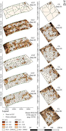
Figure 2.
Digital map indicating the absence and presence of cattle dung in the different areas (CL, crop–livestock and CLT, crop–livestock–tree systems). Dark brown represents areas with high concentration of dung, whereas the white indicates areas without cattle dung. Axes X and Y with UTM coordinates (in metres).
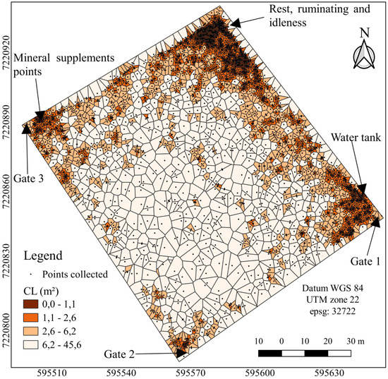
Figure 3.
Thiessen areas of the spatial distribution of the dung, in the different systems: CL, crop–livestock, considering all samples. Dark brown represents areas with high concentration of cattle dung, whereas the white indicates areas without cattle dung. Axes X and Y with UTM coordinates (m).
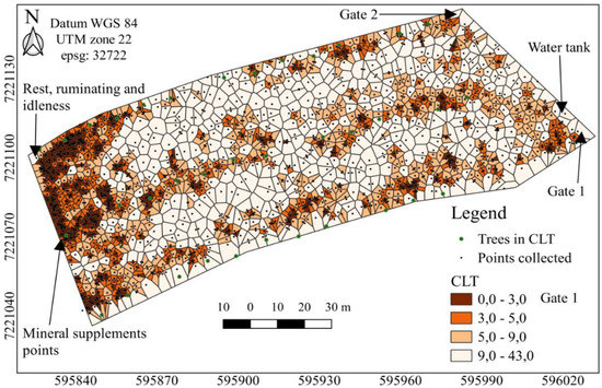
Figure 4.
Thiessen areas of the spatial distribution of the dung, in the different systems: CLT, crop–livestock–tree systems, considering all samples. Dark brown represents areas with high concentration of cattle dung, whereas the white indicates areas without cattle dung. Axes X and Y with UTM coordinates (m).
The geostatistical parameters of the Thiessen areas in the evaluations performed are shown, depending on the different ICLS (Table 4). It is observed that the data adjusted to the different models with a strong Spatial Dependence Degree (SPD). The range varied from 12 to 84 m, for the CLT (Table 4). It must be considered that Sampling 1 was performed one day after the animals entered. Considering all the samples, the range was 31 and 25 m for the CL and CLT, respectively. The semivariogram shows the spatial distribution of the cattle dung, considering all samples, in the different ICLS (See Figure A1 in Appendix A). A decrease is visible in the semivariogram over the short and long distances and an increase in the semivariogram is observed at medium distances.
Table 4.
Geostatistical models of the Thiessen areas in each sampling period, in the different integrated crop–livestock systems (CL, crop–livestock and CLT, crop–livestock–tree systems).
3.3. Initial Dry Matter of the Cattle Dung and its Quality
No differences were observed between the systems for the initial N, P, K and S concentrations in the cattle dung (Table 5). In fact, N was the nutrient having the major initial concentrations in the cattle dung, regardless of the ICLS (Table 5). Potassium was the nutrient present in a lower concentration in the cattle dung at the end (84 days) of the grassland phase.
Table 5.
Initial dry matter (DM) residue from the cattle dung and nutrient (N–P–K and S) concentrations (means ± standard error) for each system (CL, crop–livestock and CLT, crop–livestock–tree systems) and for time (1, 7, 14, 21, 28, 56 and 84 days after grazing commenced).
3.4. Dry Matter Decomposition of the Cattle Dung Residues and Nutrient Release
Dry matter loss from the cattle dung was described by the single exponential decay model for all systems (Figure 5). The act of the DM from the cattle dung residue that decomposed was ~80% (CL and CLT), and the res was ~20% (Figure 5). However, the k ranged from 0.04 (CL) to 0.02 (CLT) day−1. Consequently, the t1/2 of initial residue ranged from 17 (CL) to 29 (CLT).
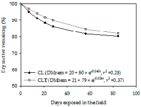
Figure 5.
Dry matter remaining (%) from the cattle dung residue, during exposure into the pasture (i.e., Lolium multiflorum + Avena strigosa) as affected by the systems (CL, crop–livestock and CLT, crop–livestock–tree). Dry matter or N, P, K and S remaining (rem) = res + act e−kt. res, resistant fraction; act, active fraction; k, non–linear decay rate; t, time; r², coefficient of determination.
The act of N ranged from 34% (CL) to 39% (CLT) while the k of N ranged from 0.03 (CL) to 0.04 (CLT) day−1, in the cattle dung residue (Figure 6). Consequently, the days required to release 50% of the initial N from the cattle dung residue ranged from 22 (CL) to 18 (CLT).
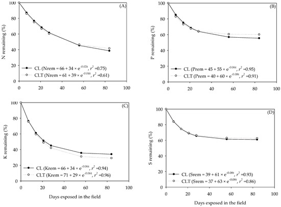
Figure 6.
Nitrogen (N), phosphorus (P), potassium (K) and sulphur (S) remaining from the cattle dung residue, during exposure into the pasture (i.e., Lolium multiflorum + Avena strigosa; A, B, C and D) as affected by the systems (CL, crop–livestock and CLT, crop–livestock–trees). Dry matter or N, P, K and S remaining (rem) = res + act e−kt. res, resistant fraction; act, active fraction; k, non–linear decay rate; t, time; r², coefficient of determination.
A few days were required to release 50% of the initial P and S, that is, the t1/2 were 12 days (CL) and 9 days (CLT) for P, and 9 days (CL) and 8 days (CLT) for S (Figure 6) for the cattle dung residues. Phosphorus and sulphur were the nutrients showing high concentrations at the end (84 days) of the incubation period; this is, on average, 55% (CL) and 60% (CLT) for P, and 61% (CL) and 63% (CLT) for S (Figure 6) for the cattle dung residues.
The t1/2 of K ranged from 11 days (CL) to 12 days (CLT) for the cattle dung residue. Potassium was the nutrient showing a lower concentration at the end (84 days) of the incubation period, that is, on average, 34% (CL) and 29% (CLT) for the cattle dung residues.
The largest nutrient releases occurred in CL (Figure 7). For instance, the total P released from the cattle dung (on day 84) and potentially available to the systems was about two times greater in the CL system (1.4 kg P ha−1) than in the CLT (0.7 kg P ha−1; Figure 7) due to the differences in the total quantity of cattle dung and number of animals (Table 2). The total N, P, K and S released from the cattle dung residues was lower in the CLT (2.2 kg ha−1 of N; 0.7 kg ha−1 of P; 2.2 kg ha−1 of K and 0.6 kg ha−1 of S), compared to that of the CL (4.2 kg ha−1 of N; 1.4 kg ha−1 of P; 3.6 kg ha−1 of K and 1.1 kg ha−1 of S) (Figure 7), i.e., a ICLS, and must be considered in the fertilisation management.
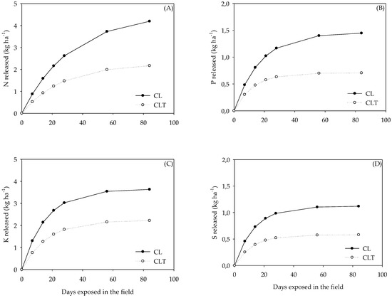
Figure 7.
Nitrogen (N), phosphorus (P), potassium (K) and sulphur (S) released (kg ha−1) from the cattle dung residue, during exposure into the pasture (i.e., Lolium multiflorum + Avena strigosa; A, B, C and D) as affected by the systems (CL, crop–livestock and CLT, crop–livestock–tree).
4. Discussion
4.1. Pasture and Animal Production
The observation of a higher Gha in the CL, compared to the CLT systems (Table 2), can be explained by the greater herbage mass throughout the winter, increasing the pasture carrying capacity. However, in 2018, both in the CL and in CLT systems, the Gha fell far below the potential of the annual cool season pastures in the ICLS, due to the lower availability of rainfall during the winter (particularly in July, see Table 1). Values of ~490 kg LW ha−1 [35] and 370 kg LW ha−1 [28] have been observed for a mixture of black oat and ryegrass in the ICLS when the targeted SH was 20 cm.
Lower animal performance in the CLT systems could be linked to both the shade effect and difficulty in maintaining the target SH, particularly in the CLT system (14 cm of sward height). Periods with SH below the targeted SH (i.e., 20 cm), during periods with stress, could be responsible for lower animal performance through bite mass limitation [36]. A lower SR was also observed under trees (Table 2). The presence of trees leads to changes in structural sward characteristics (e.g., a reduction in tiller density), changing the relationship between herbage mass and SH [37]. The consequence is a lower herbage mass under trees than those systems without trees, regardless of the SH [37]. Therefore, in order to maintain the same SH in both systems (i.e., CL and CLT), with different herbage mass, the number of animals (i.e., SR) in the CLT system was reduced.
Therefore, to maintain a greater SR on the CLT system, it is necessary to manage the trees (thinning and pruning) over time to avoid very large impacts on pasture productivity, in order to maintain the targeted SH and optimize animal performance. Further, to increase the efficiency of the CLT, beyond moderate grazing (i.e., 20 cm), moderate shade (35–37%, according to [38]) must be adopted (e.g., by increasing the frequency of thinning), [39] in order to decrease the negative effects on pasture growth and animal performance [38].
After 12 years of introduction of the tree component, the greatest light restriction, caused by the tree growth was the determinant for the differences observed between the systems. Long–term studies in the ICLS, particularly with trees, are important to ascertain the system viability, as well as to determine the need for the management of the tree component (i.e., thinning), in order to maintain the production diversification and income generation of the agricultural property.
4.2. Distribution of Cattle Dung
The range of area covered by each cattle dung here (i.e., 0.03 ± 0.01 m2) is below the values reported by other authors, which extended from 0.05 to 0.09 m2 [40]; ~0.05 m2 [41] and 0.12 m2 [20]. However, the percentage of the dung-covered pasture surface, considering all samples, was similar to the magnitudes observed in other experiments (<1% in 10 weeks of grazing, [41]). The area covered by faeces represented only 0.7 and 0.5% for the CL and CLT, respectively, of the total pasture area during the 14-week experimental period. These values are directly related to the stocking rate. Although dung patches may cover only little surface of the grassland, the associated high nutrient input induces pasture growth, and these regions may contribute to ~70% of the annual pasture production [40].
The number of cattle dung per animal per day (9 ± 1 defaecations/animal per day) does not differ between the systems; however, they are below the values reported by other authors, i.e., between 11 and 16 [40], 10.8 [20]; and 9.8 defaecations per day [42]. The number of defecations per day can be influenced by the environmental factors and grazing conditions [40].
However, between 2,652 and 1,810 cattle dung were recorded in the CL and CLT systems, respectively, during the evaluations. It is known that the faecal production is correlated with consumption and this, in turn, with animal performance [3]. In the CLT system, with a high level of light restriction, animal performance was reduced when compared to the CL system. The consequence of this was the great differences found between the systems for the total production of cattle dung.
As the average frequency of defaecation was 9 ± 1 defaecations/animal per day and the average dung weight at each defaecation was of 170 ± 18 g DM, the estimated daily faecal excretion was 1.5 kg DM per animal per day. Thus, considering the stocking rate of three animals per hectare in the CL and two animals per hectare in the CLT system (Table 3), and the 105-day grazing period, in the present study, over the grazing period, the total dry mass of cattle dung deposited on the soil surface was 477 and 318 kg of DM in the CL and CLT systems, respectively.
The geostatistical analysis of the Thiessen areas adjusted different models to the semivariogram throughout the evaluations (Table 4), revealing that the animals deposit their dung in different positions during each period, also evidenced by the different ranges of spatial dependence of the data. The higher the range values (Table 4) the greater the spatial continuity in the distribution of cattle dung by the area, while, the lower the values, the less the spatial continuity conferred in the dung distribution, as explained by the dung deposition in attractive sites. Despite this, when all the samplings are considered, and the different models (Table 4) are added over time, a visual pattern is presented in the behaviour of the spatial distribution of the cattle dung, among the ICLS (Figure A1). However, differences are observed in the semivariogram and distances, due to the different areas and paddock shapes. Validation studies of the semivariogram analysis (Figure A1) enabled the observation that the deposition of cattle dung follows a clear distribution pattern in relation to the attractive points, as was also reported by other authors [20,22,31,40,43]. In the CLT, the distribution was more uniform when trees were present (9 × 28 m), which is evident by the lower reach in the semivariogram adjusts for the CLT (25 m) in relation to the CL (30 m), when considering the Thiessen areas formed from the concentration points (Figure 3 and Figure 4).
In tropical conditions, the trees available in the pastures affect spatial distribution of the dung, stimulating homogeneity [22]. This behaviour may be caused by the fact that the animals prefer to spend most of the day under the shade of the trees, in a tropical climate [23], leading to homogeneous nutrient return and concentration in pasture areas, such as close to the shade and water areas [13]. Consequently, in the CLT system, the dung patches were distributed close to the shaded areas. These shaded places were the favourite places for the heifers to ruminate and idle away the time, when they defaecated more [23]. In fact, the behaviour of the animals observed in our study, i.e., in a subtropical region, was like that observed in the tropical climates, contrary to our initial hypothesis. Thus, shady areas in the pastures, with well distributed trees throughout these areas, are recommended for subtropical conditions to improve the spatial distribution of cattle dung in the area.
The CL system present higher concentrations of dung at sites near the rest areas (for ruminating and idleness), mineral supplement points, water troughs and fences opposite the gate. Consequently, the pattern in which nutrients are returned to the pasture, as the dung, is heterogeneous [18,40]. Due to this uneven pattern, probably, a nutrient build-up is observed in these areas of the campsite (gates, water troughs, mineral supplements points, socialisation areas) as well as a depletion in the nutrient in the rest of the grassland. In order to minimize these effects, an option could be an increase in the frequency of changes in the positions of the gate, fences, water troughs and mineral supplement points.
Under our experimental and subtropical conditions, as the tree arrangement was 9 × 28 m (~40 trees ha−1), there was a probably greater inclination for the animals to rest and ruminate near the trees; consequently, there is a more even distribution of dung over the experimental units, since trees were well distributed throughout the area. This probably reduces nutrient losses and favours more efficient cycling within the system.
4.3. Dry matter Decomposition and Nutrient Release of Cattle Dung Residues
The cattle dung disintegration process, that is, the disappearance of DM, occurred in a restricted manner, since an 11-mm precipitation was observed (July 2018, in the study period, Table 1). Low precipitation could have delayed the physical disintegration of the cattle dung because this process is favoured by the impact of raindrops [40], together with the microbiological activity, as the main factor responsible for the disintegration or decomposition of the dung. The low rate of cattle dung decomposition is also associated with the presence of recalcitrant constituents (~20%, Figure 5). Therefore, below 20% of the DM of the plates disappeared during the 84 days of the study. Further, in the current study, since the SH was maintained below 20 cm in CLT systems, the animals probably ingested low-quality plant parts (e.g., stem and leaf sheath, i.e., plant parts with a higher fibre and lignin content than leaves), when compared with animals in the CL system. This could help to explain the slightly difference between systems on dry matter decomposition of the cattle dung residues, with a slower degradation in CLT systems. A higher C:N ratio favours a slower decomposition.
Total quantities (kg ha−1) of N, P, K and S released from the dung residue (Figure 7) and potentially available to the actual and subsequent crop were more likely related to the quantity of dung residues which were, in general, reduced in the CLT, rather than to any changes in the dung quality due the shading effect.
Nitrogen was the nutrient present at the greatest initial concentration in cattle dung (~19 g kg−1, Table 5), probably because the more labile compartments are broken down in the animal rumen, a small amount is retained in the animal’s tissue, and most is released with urine and dung [36]. However, because mineralisation is microbially driven, several factors affect it, including temperature and soil moisture [44]. Nitrogen mineralisation increases with the rising temperature under conditions found in agricultural soils [44]. For instance, the total N released from the cattle dung residue (at 84 days) and potentially available to the actual and subsequent soybean crop was about two times greater in the CL (4 kg N ha−1) than in the CLT system (2 kg N ha−1; Figure 7) due to differences in the total quantity of cattle dung (Table 3), since a higher number of heifers were present in the CL systems (3 cattle ha−1), while a lower number (2 cattle ha−1) were present in the CLT.
As N was the nutrient present in the highest initial concentration (Table 5), the greatest N release occurred from the cattle dung residue, regardless of the systems (Figure 7). However, we should take into account that the N values released in the pasture phase were related only to the N cycling by the decomposition of a single compartment (cattle dung), and not to the great potential of the N cycling of the whole system. Nitrogen release from cattle dung can be attributed to the easily decomposable fraction by microorganisms (low C:N ratio), quality (structure) and lignin content [45,46].
Rapid P releases had been reported by [11]. Moderate grazing also caused the speedier release of P from the dung, as indicated by the lower t1/2, namely, 5 to 6 days in the labile fraction [11]. The rapid P release from the dung have been related to the quality (structure) and lower lignin content [11,45]. The phosphorus availability from cattle dung is high (>70%), as most of the dung P is inorganic and becomes plant-available [44].
The t1/2 of K released from the dung was similar to the report of [11,40]. This rapid release of K occurred because most of the K is in water-soluble form [47]. Between 60–70% of the K ingested by animals returns to the soil system [14]. These observations suggest the importance of the dynamics of K in the balance and maintenance of the system. Grazing animals significantly alter the cycling of K, mainly due to the spatial heterogeneity of K return via animal excreta [48].
A few days were necessary for the release of 50% of the initial S, that is, the t1/2 were 9 days (CL) and 8 days (CLT) for the cattle dung residue. In the initial stage, the pattern of release was rapid, after which it was constant up to 84 days. The dynamics of S is dependent on the dynamics of N. The rate of release of the available S content is dependent upon environmental conditions, initial concentrations and characteristics of the S, as well as the microbial population in the soils [49]. It might be due also to the increase in the strength of mineralisation and the increased microorganism activity during this period. These favourable conditions boost the S release. After 21 days, there was a slight reduction in the available S content, which might have been caused by the commencement of the immobilisation and hampered mineralisation, as well as the reduced microbial activity [49]. Probably, the remaining material in the field is highly resistant, i.e., with a high content of lignin and fibre, which is more difficult to decompose [50].
From these results, and considering 84 days after the entry of the animals, about ~60% of the N, ~42% of the P, ~68% of the K and ~38% of the S present in the cattle dung, in the active fraction, was completely released. This represents about 4 and 2 kg ha−1 of N; 1.4 and 0.7 kg ha−1 of P; 4 and 2 kg ha−1 of K and 1.1 and 0.6 kg ha−1 of S in the CL and CLT, respectively, released by cycling in the initial residue (Figure 7). Briefly, small quantities of N, P, K and S were cycled from cattle dung under a beef-cattle and soybean integration system but must be considered for fertilisation management practices.
The nutrient cycling could have been much higher had it not been a drought winter (Table 1). For example, a study with the CL system in the subtropics, with different heights and 120 days of grazing, showed a cycling of around 3 to 8 kg ha−1 of P and 10 to 22 kg ha−1 of K cycled by dung [11]. Thus, for instance, it has been recommended to use simple specific fertilizer sources (e.g., monoammonium phosphate (MAP), diammonium phosphate (DAP), and potassium chloride (KCl)) in ICLS, that have a high concentration of specific nutrients, rather than N–P–K formulated fertilizers, which make it possible to achieve more technically adequate management and more economic efficiency for rural producers, avoiding losses and luxury consumption [51], when also considering the nutrient cycling by residues.
Our results reinforce the importance of keeping the animals permanently in the area, in order to reduce the nutrients losses from animal excreta. Another factor that contributes to the reduction of losses from excreta is a more uniform distribution, in order to make better use by the intercropping. Further, an adequate management of grazing intensity allows greater biomass production, increasing the SR and excreta deposition. Our results, therefore, also reinforce the necessity to understand the nutrient release patterns from residues (animal and plant) over the long term, for ICLS conditions, to improve fertilisation management. Furthermore, it is imperative in the ICLS with trees to intensify silvicultural practices over time, to minimise the effect of the trees on intercropping productivity, to ensure a more constant addition of residues (from both the crop and stocking phases) and to promote productive, economic and sustainable stability of these systems [25]. Therefore, a few feasible silvicultural interventions need to be considered to avoid losses in pasture, thus maximising the number of animals and nutrient cycling benefits.
It is recommended to use ICLS systems with trees because, in addition to contributing to nutrient cycling, these systems are particularly important to recovery of degraded areas, especially in steep areas, since tree lines contribute to soil conservation. Further, ICLS with trees makes it possible to increase income diversification for the producer, making more sustainable agriculture, and being a technology fully in line with the goals of the Brazilian government in the Low Carbon Agriculture (ABC) program.
5. Conclusions
The pattern in which the nutrients are returned to the pasture in the form of dung is nonuniform for the crop–livestock system. The crop–livestock–tree system shows a more homogeneous spatial dung distribution, despite a few small points of concentration which continue to remain in areas, such as around the cow drinkers and the gate.
The integrated crop–livestock systems had no effect upon the decomposition and release dynamics for nitrogen, phosphorus, potassium, and sulphur. However, the total nitrogen, phosphorus, potassium and sulphur released from the cattle dung and which was potentially available for the crops varied according to the integrated crop–livestock system, depending on the number of animals present during the grazing period and the quantity of the cattle dung.
Author Contributions
The five co–editors equally contributed to organising the special issue, editorial work, and the writing of this editorial. All authors have read and agreed to the published version of the manuscript.
Funding
This work forms part of a cooperation agreement (No. 21500.10/0008–2) between the IAPAR and Embrapa Forestry.
Acknowledgments
The authors extend their gratitude to Giliardi Stafin and Atila Cristian Santana for the technical support and Luis Miguel Schiebelbein and Alisson Marcos Fogaça for the valuable statistical comments. The second and last authors are grateful to CNPq for the award of fellowships #482 310903/2018–1 and # 305803/2018–2, respectively.
Conflicts of Interest
The authors declare no conflict of interest. The funders had no role in the design of the study; in the collection, analyses, or interpretation of data; in the writing of the manuscript, or in the decision to publish the results.
Appendix A

Figure A1.
Semivariogram of the Thiessen areas of the spatial distribution of cattle dung, for the different ICLS: (A) crop–livestock, CL and (B) crop–livestock–tree CLT, considering all evaluations.
References
- Pretty, J. Intensification for redesigned and sustainable agricultural systems. Science 2018, 362, 1–7. [Google Scholar] [CrossRef] [PubMed]
- Lawson, G.; Dupraz, C.; Watté, J. Can Silvoarable Systems Maintain Yield, Resilience, and Diversity in the Face of Changing Environments? In Agroecosystem Diversity; Elsevier: Amsterdam, The Netherlands, 2019; pp. 145–168. ISBN 978-0-12-811050-8. [Google Scholar]
- De Faccio Carvalho, P.C.; Anghinoni, I.; de Moraes, A.; de Souza, E.D.; Sulc, R.M.; Lang, C.R.; Flores, J.P.C.; Terra Lopes, M.L.; da Silva, J.L.S.; Conte, O.; et al. Managing grazing animals to achieve nutrient cycling and soil improvement in no-till integrated systems. Nutr. Cycl. Agroecosyst. 2010, 88, 259–273. [Google Scholar] [CrossRef]
- Neely, C.; Fynn, A. Critical Choices for Crop and Livestock Production Systems That Enhance Productivity and Build Ecosystem Resilience; SOLAW Background Thematic Report–TR11; FAO: Rome, Italy, 2012; p. 38. [Google Scholar]
- Bélanger, J.; Pilling, D. The State of the World’s Biodiversity for Food and Agriculture; Commission on Genetic Resources for Food and Agriculture: Rome, Italy; Food and Agriculture Organization of the United Nations: Rome, Italy, 2019; ISBN 978-92-5-131270-4. [Google Scholar]
- De Notaro, K.A.; de Medeiros, E.V.; Duda, G.P.; Silva, A.O.; de Moura, P.M. Agroforestry systems, nutrients in litter and microbial activity in soils cultivated with coffee at high altitude. Sci. Agric. 2014, 71, 87–95. [Google Scholar] [CrossRef]
- Cavagnaro, J.B.; Trione, S.O. Physiological, morphological and biochemical responses to shade of Trichloris crinita, a forage grass from the arid zone of Argentina. J. Arid Environ. 2007, 68, 337–347. [Google Scholar] [CrossRef]
- Da Pontes, L.S.; Giostri, A.F.; Baldissera, T.C.; Barro, R.S.; Stafin, G.; Porfírio-da-Silva, V.; Moletta, J.L.; César de Faccio Carvalho, P. Interactive Effects of Trees and Nitrogen Supply on the Agronomic Characteristics of Warm-Climate Grasses. Agron. J. 2016, 108, 1531–1541. [Google Scholar] [CrossRef]
- Guo, L.B.; Sims, R.E.H. Effects of light, temperature, water and meatworks effluent irrigation on eucalypt leaf litter decomposition under controlled environmental conditions. Appl. Soil Ecol. 2001, 17, 229–237. [Google Scholar] [CrossRef]
- Quinkenstein, A.; Wöllecke, J.; Böhm, C.; Grünewald, H.; Freese, D.; Schneider, B.U.; Hüttl, R.F. Ecological benefits of the alley cropping agroforestry system in sensitive regions of Europe. Environ. Sci. Policy 2009, 12, 1112–1121. [Google Scholar] [CrossRef]
- Assmann, J.M.; Martins, A.P.; Anghinoni, I.; de Oliveira Denardin, L.G.; de Holanda Nichel, G.; de Andrade Costa, S.E.V.G.; Pereira e Silva, R.A.; Balerini, F.; de Faccio Carvalho, P.C.; Franzluebbers, A.J. Phosphorus and potassium cycling in a long-term no-till integrated soybean-beef cattle production system under different grazing intensities insubtropics. Nutr. Cycl. Agroecosyst. 2017, 108, 21–33. [Google Scholar] [CrossRef]
- Braz, S.P.; do Nascimento Junior, D.; Cantarutti, R.B.; Regazzi, A.J.; Martins, C.E.; da Fonseca, D.M. Disponibilização dos Nutrientes das Fezes de Bovinos em Pastejo para a Forragem. Rev. Bras. Zootec. 2002, 31, 1614–1623. [Google Scholar] [CrossRef][Green Version]
- Dubeux, J.C.B.; Sollenberger, L.E.; Vendramini, J.M.B.; Interrante, S.M.; Lira, M.A. Stocking Method, Animal Behavior, and Soil Nutrient Redistribution: How are They Linked? Crop Sci. 2014, 54, 2341–2350. [Google Scholar] [CrossRef]
- Rodrigues, A.M.; Cecato, U.; Fukumoto, N.M.; Galbeiro, S.; dos Santos, G.T.; Barbero, L.M. Concentrações e quantidades de macronutrientes na excreção de animais em pastagem de capim-mombaça fertilizada com fontes de fósforo. Rev. Bras. Zootec. 2008, 37, 990–997. [Google Scholar] [CrossRef][Green Version]
- Da Silva, V.B.; da Silva, A.P.; de Dias, B.O.; Araujo, J.L.; Santos, D.; Franco, R.P. Decomposição e liberação de N, P e K de esterco bovino e de cama de frango isolados ou misturados. Rev. Bras. Ciência Solo 2014, 38, 1537–1546. [Google Scholar] [CrossRef]
- Souto, P.C.; Souto, J.S.; Santos, R.V.; Araújo, G.T.; Souto, L.S. Decomposição de estercos dispostos em diferentes profundidades em área degradada no semi-árido da Paraíba. Rev. Bras. Ciência Solo 2005, 29, 125–130. [Google Scholar] [CrossRef]
- Sun, Y.; He, X.Z.; Hou, F.; Wang, Z.; Chang, S. Grazing Elevates Litter Decomposition But Slows Nitrogen Release in an Alpine Meadow. Biogeosci. Discuss 2018. under review. [Google Scholar] [CrossRef]
- Vendramini, J.M.B.; Silveira, M.L.A.; Dubeux, J.C.B., Jr.; Sollenberger, L.E. Environmental impacts and nutrient recycling on pastures grazed by cattle. Rev. Bras. Zootec. 2007, 36, 139–149. [Google Scholar] [CrossRef]
- Ferreira, L. The effect of different shading availabilities dispersion of feces of cattle in the pastures. Rev. Bras. Agroecol. 2011, 6, 137–146. [Google Scholar]
- White, S.L.; Sheffield, R.E.; Washburn, S.P.; King, L.D.; Green, J.T. Spatial and Time Distribution of Dairy Cattle Excreta in an Intensive Pasture System. J. Environ. Qual. 2001, 30, 2180–2187. [Google Scholar] [CrossRef]
- Da Silva, F.D.; Amado, T.J.C.; Bredemeier, C.; Bremm, C.; Anghinoni, I.; de Faccio Carvalho, P.C. Pasture grazing intensity and presence or absence of cattle dung input and its relationships to soybean nutrition and yield in integrated crop–livestock systems under no-till. Eur. J. Agron. 2014, 57, 84–91. [Google Scholar] [CrossRef]
- Carnevalli, R.A.; de Mello, A.C.T.; Shozo, L.; Crestani, S.; Coletti, A.J.; Eckstein, C. Spatial distribution of dairy heifers’ dung in silvopastoral systems. Ciência Rural 2019, 49, 1–9. [Google Scholar] [CrossRef]
- Giro, A.; Pezzopane, J.R.M.; Barioni Junior, W.; de Pedroso, A.F.; Lemes, A.P.; Botta, D.; Romanello, N.; do Barreto, A.N.; Garcia, A.R. Behavior and body surface temperature of beef cattle in integrated crop-livestock systems with or without tree shading. Sci. Total Environ. 2019, 684, 587–596. [Google Scholar] [CrossRef]
- USDA. United States Department of Agriculture Soil Taxonomy: A Basic System of Soil Classification for Making and Interpreting Soil Surveys; USDA: Washington, DC, USA, 1999.
- Carpinelli, S.; da Fonseca, A.F.; Assmann, T.S.; da Pontes, L.S. Effects of trees and nitrogen supply on macronutrient cycling in integrated crop–livestock systems. Agron. J. 2020, 112, 1377–1390. [Google Scholar] [CrossRef]
- Porfírio-da-Silva, V.; de Moraes, A.; Moletta, J.L.; da Pontes, L.S.; de Oliveira, E.B.; Pelissari, A.; de Carvalho, P.C.F. Danos causados por bovinos em diferentes espécies arbóreas recomendadas para sistemas silvipastoris. Pesqui. Florest. Bras. 2012, 32, 67–76. [Google Scholar] [CrossRef]
- Mott, G.O.; Lucas, H.L. The design, conduct and interpretation of grazing trials on cultivated and improved pastures. In Proceedings of the Sixth International Grassland Congress, State College, PA, USA, 17–23 August 1952; Volume 6, pp. 1380–1395. [Google Scholar]
- Da Pontes, L.S.; Barro, R.S.; Savian, J.V.; Berndt, A.; Moletta, J.L.; Porfírio-da-Silva, V.; Bayer, C.; de Faccio Carvalho, P.C. Performance and methane emissions by beef heifer grazing in temperate pastures and in integrated crop-livestock systems: The effect of shade and nitrogen fertilization. Agric. Ecosyst. Environ. 2018, 253, 90–97. [Google Scholar] [CrossRef]
- Abreu, M.F.; Silva, F.C.; Coscione, A.R.; Andrade, C.A.; Andrade, J.C.; Santos, G.C.G.; Abreu Junior, C.H.; Gomes, T.F. Análise Química de Fertilizantes Orgânicos (urbanos). In Manual de Análises Químicas de Solos; Da Silva, F.C., Ed.; Plantas e Fertilizantes: Brasília, Brazil, 2009; ISBN 978-85-7383-430-7. [Google Scholar]
- Goovaerts, P. Geostatistical approaches for incorporating elevation into the spatial interpolation of rainfall. J. Hydrol. 2000, 228, 113–129. [Google Scholar] [CrossRef]
- Auerswald, K.; Mayer, F.; Schnyder, H. Coupling of spatial and temporal pattern of cattle excreta patches on a low intensity pasture. Nutr. Cycl. Agroecosyst. 2010, 88, 275–288. [Google Scholar] [CrossRef]
- Fanchi, J. Integrated Reservoir Asset Management: Principles and Best Practices, 1st ed.; Gulf Professional Publishing: Houston, TX, USA, 2010; ISBN 0-12-382089-8. [Google Scholar]
- Beltrame, R.A.; Lopes, J.C.; de Lima, J.S.S.; Quinto, V.M. Spatial distribution of physiological quality of Joannesia princeps Vell. SEEDS1. Rev. Árvore 2018, 41. [Google Scholar] [CrossRef]
- Cambardella, C.A.; Moorman, T.B.; Novak, J.M.; Parkin, T.B.; Karlen, D.L.; Turco, R.F.; Konopka, A.E. Field-Scale Variability of Soil Properties in Central Iowa Soils. Soil Sci. Soc. Am. J. 1994, 58, 1501–1511. [Google Scholar] [CrossRef]
- Lopes, M.L.T.; de Carvalho, P.C.F.; Anghinoni, I.; dos Santos, D.T.; Kuss, F.; de Freitas, F.K.; Flores, J.P.C. Sistema de integração lavoura-pecuária: Desempenho e qualidade da carcaça de novilhos superprecoces terminados em pastagem de aveia e azevém manejada sob diferentes alturas. Ciência Rural 2008, 38, 178–184. [Google Scholar] [CrossRef]
- Carvalho, P.C.D.F. Harry Stobbs Memorial Lecture: Can grazing behavior support innovations in grassland management? Trop. Grassl. Forrajes Trop. 2013, 1, 137. [Google Scholar] [CrossRef]
- Da Pontes, L.S.; Carpinelli, S.; Stafin, G.; Porfírio-da-Silva, V.; dos Santos, B.R.C. Relationship between sward height and herbage mass for integrated crop-livestock systems with trees. Grassl. Sci. 2017, 63, 29–35. [Google Scholar] [CrossRef]
- Pang, K.; Van Sambeek, J.W.; Navarrete-Tindall, N.E.; Lin, C.-H.; Jose, S.; Garrett, H.E. Responses of legumes and grasses to non-, moderate, and dense shade in Missouri, USA. I. Forage yield and its species-level plasticity. Agrofor. Syst. 2019, 93, 11–24. [Google Scholar] [CrossRef]
- Da Pontes, L.S.; Stafin, G.; Moletta, J.L.; Porfírio-da-Silva, V. Performance of Purunã beef heifers and pasture productivity in a long-term integrated crop-livestock system: The effect of trees and nitrogen fertilization. Agrofor. Syst. 2020. [Google Scholar] [CrossRef]
- Haynes, R.J.; Williams, P.H. Nutrient Cycling and Soil Fertility in the Grazed Pasture Ecosystem. In Advances in Agronomy; Elsevier: Amsterdam, The Netherlands, 1993; Volume 49, pp. 119–199. ISBN 978-0-12-000749-3. [Google Scholar]
- Braz, S.P.; do Nascimento Júnior, D.; Cantarutti, R.B.; Martins, C.E.; da Fonseca, D.M.; Barbosa, R.A. Caracterização da distribuição espacial das fezes por bovinos em uma pastagem de Brachiaria decumbens. Rev. Bras. Zootec. 2003, 32, 787–794. [Google Scholar] [CrossRef]
- Braz, S.P.; do Nascimento Junior, D.; Cantarutti, R.B.; Regazzi, A.J.; Martins, C.E.; da Fonseca, D.M.; Barbosa, R.A. Aspectos quantitativos do processo de reciclagem de nutrientes pelas fezes de bovinos sob pastejo em pastagem de Brachiaria decumbens na Zona da Mata de Minas Gerais. Rev. Bras. Zootec. 2002, 31, 858–865. [Google Scholar] [CrossRef]
- Bailey, D.W.; Welling, G.R.; Miller, E.T. Cattle use of foothills rangeland near dehydrated molasses supplement. JRM 2006, 54, 338–347. [Google Scholar] [CrossRef]
- Eghball, B.; Wienhold, B.J.; Gilley, J.E.; Eigenberg, R.A. Mineralization of manure nutrients. J. Soil Water Conserv. 2002, 57, 470–473. [Google Scholar]
- Semmartin, M.; Garibaldi, L.A.; Chaneton, E.J. Grazing history effects on above- and below-ground litter decomposition and nutrient cycling in two co-occurring grasses. Plant Soil 2008, 303, 177–189. [Google Scholar] [CrossRef]
- Assmann, J.M.; Anghinoni, I.; Martins, A.P.; de Costa, S.E.V.G.A.; Kunrath, T.R.; Bayer, C.; de Carvalho, P.C.F.; Franzluebbers, A.J. Carbon and nitrogen cycling in an integrated soybean-beef cattle production system under different grazing intensities. Pesqui. Agropecuária Bras. 2015, 50, 967–978. [Google Scholar] [CrossRef]
- Esse, P.C.; Buerkert, A.; Hiernaux, P.; Assa, A. Decomposition of and nutrient release from ruminant manure on acid sandy soils in the Sahelian zone of Niger, West Africa. Agric. Ecosyst. Environ. 2001, 83, 55–63. [Google Scholar] [CrossRef]
- Mathews, B.W.; Sollenberger, L.E.; Nkedi-Kizza, P.; Gaston, L.A.; Hornsby, H.D. Soil Sampling Procedures for Monitoring Potassium Distribution in Grazed Pastures. Agron. J. 1994, 86, 121–126. [Google Scholar] [CrossRef]
- Department of Soil Science and Agricultural Chemistry, College of Cgriculture, PJTSAU; Venugopal, G. Release Pattern of Available Sulphur and Sulphur Fractions Influenced by Elemental Sulphur and Poultry Manure in Different Soils of Norther Telangana. Int. J. Pure Appl. Biosci. 2017, 5, 1606–1610. [Google Scholar] [CrossRef]
- Whitehead, D.C. Nutrient Elements in Grassland: Soil-Plant-Animal Relationships; Cabi: Wallingford, UK, 2000; ISBN 0-85199-938-7. [Google Scholar]
- Bernardon, A.; Assmann, T.S.; Brugnara Soares, A.; Franzluebbers, A.; Maccari, M.; de Bortolli, M.A. Carryover of N-fertilization from corn to pasture in an integrated crop-livestock system. Arch. Agron. Soil Sci. 2020, 1–16. [Google Scholar] [CrossRef]
© 2020 by the authors. Licensee MDPI, Basel, Switzerland. This article is an open access article distributed under the terms and conditions of the Creative Commons Attribution (CC BY) license (http://creativecommons.org/licenses/by/4.0/).