Article

Comparison of Frequentist and Bayesian Meta-Analysis Models for Assessing the Efficacy of Decision Support Systems in Reducing Fungal Disease Incidence

by
Elena Lázaro
1,*,
David Makowski
2,3,
Joaquín Martínez-Minaya
4 and
Antonio Vicent
1
1
Centre de Protecció Vegetal i Biotecnologia, Institut Valencià d’Investigacions Agràries (IVIA), 46113 Moncada, Valencia, Spain
2
INRA, UMR 211 INRA AgroParisTech Université Paris-Saclay, 78850 Thiverval-Grignon, France
3
CIRED, CIRAD, 94130 Nogent-sur-Marne, France
4
BCAM—Basque Center for Applied Mathematics, Mazarredo, 14 E48009 Bilbao, Basque Country, Spain
*
Author to whom correspondence should be addressed.
Agronomy 2020, 10(4), 560; https://doi.org/10.3390/agronomy10040560
Submission received: 20 March 2020 / Accepted: 3 April 2020 / Published: 13 April 2020

Abstract

:
Diseases of fruit and foliage caused by fungi and oomycetes are generally controlled by the application of fungicides. The use of decision support systems (DSSs) may assist to optimize fungicide programs to enhance application on the basis of risk associated with disease outbreak. Case-by-case evaluations demonstrated the performance of DSSs for disease control, but an overall assessment of the efficacy of DSSs is lacking. A literature review was conducted to synthesize the results of 67 experiments assessing DSSs. Disease incidence data were obtained from published peer-reviewed field trials comparing untreated controls, calendar-based and DSS-based fungicide programs. Two meta-analysis generic models, a “fixed-effects” vs. a “random-effects” model within the framework of generalized linear models were evaluated to assess the efficacy of DSSs in reducing incidence. All models were fit using both frequentist and Bayesian estimation procedures and the results compared. Model including random effects showed better performance in terms of AIC or DIC and goodness of fit. In general, the frequentist and Bayesian approaches produced similar results. Odds ratio and incidence ratio values showed that calendar-based and DSS-based fungicide programs considerably reduced disease incidence compared to the untreated control. Moreover, calendar-based and DSS-based programs provided similar reductions in disease incidence, further supporting the efficacy of DSSs.

1. Introduction

According to Higgins et al. [1], “meta-analysis refers to the statistical synthesis of results from a series of studies”. In plant pathology, meta-analysis has become in a powerful tool  [2] to address questions such as factors determining the effects of different pesticides and biological treatments for managing diseases [3,4,5]. Meta-analysis implementation requires the selection of proper statistical models to draw robust conclusions. Different types of statistical models were proposed with that regard; however, there is a risk of biased parameter estimation, misinterpretation and incorrect conclusions if a quality control of statistical techniques is not considered [6]. According to Philibert  et  al. [7], one of the quality control measures which meta-analysis should incorporate is a sensitivity study of the estimated effects in relation to the statistical model characteristics.
In practice, the selection of a statistical model rises two important issues: (i) the nature of the measured variable (continuous, binary, categorical) and (ii) the consideration between-experiments variability in the measured variable which leads to the choice between fixed and random effects models [1,8,9]. Furthermore, model type will determine the “treatment effect” (also named“effect size”) choice to summary effects and assess differences between treatments evaluated. In plant pathology, meta-analysis sensitivity analyses addressed differences between fixed-effect and random-effect models within different modelling frameworks (linear models, generalized linear models)  [3,5] and also for frequentist vs. Bayesian inferential approaches [5].
In this paper, we consider experiments where the measured variable is binary and corresponds to the occurrence of a disease in treated/untreated plant materials. Within this framework, a sensitivity analysis between two different meta-analysis models (fixed effects vs. random effects) and two different estimation methods (frequentist vs. Bayesian) were proposed from a generic generalized lineal model (GLM) [10] to assess the efficacy of fungicide programs based on decision support systems (DSSs) in comparison to standard calendar-based programs.
Currently, agricultural policies promote the adoption of more sustainable low-input agricultural systems reinforcing the reduction of fungicide application among other measures. In that context, the use of predictive models (empirical or process-based) allows estimating the risk of disease and devise more efficient fungicide spray programs optimizing spray timing and avoiding unnecessary treatments  [11,12]. Building on predictive models, DSS programs integrate all types of information required for control decisions, including action thresholds [11]. However, the level of adoption of them is generally low [13]. The perceived lack of reliability of DSSs could be overcome with more studies comparing the efficacy of this strategy with the standard calendar-based fungicide programs. In this context, meta-analysis is a powerful methodology in the sense that can combine different sources of information covering a wide range of disease-crop systems.
In this paper, we compare four different GLMs to perform a meta-analysis on the efficacy of DSS and calendar fungicide programs. The four models differ in the assumption made on the variability of the treatment effect (which is assumed to be either constant or variable between experiments) and in the inferential method used for parameter estimation (frequentist or Bayesian). For all models, three treatment effects measures: disease incidence, odds ratios and incidence ratios were estimated and compared to evaluate the efficacy of DSS and calendar fungicide programs.

2. Material and Methods

2.1. Literature Search and Data

A database was assembled based on a systematic literature review from the (i) Web of Science (WOS) and (ii) the Fungicide and Nematicide Tests (F&N Tests and Plant Disease management reports). For (i), publications were selected according to multiple search strings described in Appendix A. For (ii), reports were extracted according to multiple key words (Appendix A). Hard copies of volumes published prior to 2000 were examined directly. Relevant experiments were selected according the following criteria: (a) the experiment evaluated at least one DSS-based strategy, one calendar-based strategy and an untreated control (as  a minimum each experiment included three sub-experiments according to the type of treatment); (b)  all sub-experiments reported disease incidence (i.e., proportion of diseased organs) and sample size (i.e., total of organs considered to evaluate disease incidence). All experiments fulfilling those criteria were included in the meta-analysis. In calendar-based programs the number and timing of fungicide applications was fixed before the experiment, usually based on the standard practices for disease control. In DSS-based programs the number and timing of fungicide applications was decided during the course of the experiment based on risk indicators.
Each experiment was defined as a unique combination of location (country, state), year, crop, organ evaluated, disease, pathogen, treatment strategy, number of sprays and treatment id (see Table A2 for detailed information about the location, crop and disease information). Conversely, each  sub-experiment was characterised by the type of treatment (DSS, calendar or untreated), the  observed disease incidence, the sample size and the number of sprays. For both sources ((i) and (ii)) a total of 67 experiments, 285 sub-experiments were selected from a total of 19 publications/reports (see Table A3 for further details). The number of independent experiments among the papers varied from 1 to 11 and the number of sub-experiments among experiments from 3 to 7 (Table A3). The database included a total of 67 sub-experiments under untreated conditions, 86 under a calendar-based strategy and 132 under DSS-based strategy (Table A3). An overall and individual (per sub-experiment) description of the dataset is provided in Section 3.1 in terms of the observed disease incidence and incidence ratios (IRs) between calendar (Cal./Unt.) and DSS (DSS/Unt.) strategies against the untreated control.

2.2. Meta-Analysis

The response variable used to quantify the level of disease in all experiments (sub-experiments) was the number of diseased organs. Given the nature of this metric, meta-analysis was formulated within the familiar framework of GLMs [10] and applied to data with a binomial likelihood [14] and a logit link function. The GLM overcomes problems of models based on normal likelihood [15]. It was formulated to compare the effect of the two fungicide strategies (DSS and calendar) simultaneously in comparison to the untreated control.
This generic model was extended by the inclusion of random effects usually named as generalised linear mixed model (GLMM) [16] with the aim to account for the unobserved sources of variability among experiments beyond the fungicide treatment effects, such as the different pathogens/crops targeted, the mode of action of the fungicides, and inoculum levels. Both GLM and GLMM were fitted using two statistical methods, a frequentist and a Bayesian method. All implementations were made in the R environment (version 3.5.1). The full analysis can be reproduced using code and data archived at https://bitbucket.org/elaher/comparative-meta-analysis/src/master/.

Statistical Modelling

The logistic GLM was formulated as:
Y i j Binomial ( n i j , θ i j ) ,
logit ( θ i j ) = log θ i j 1 θ i j = β 0 + β cal I cal ( ij ) + β dss I dss ( ij ) ,
where the random variable Y i j which describes the number of diseased organs in the sub-experiment j of the experiment i out of a total of n i j organs analyzed, is assumed to follow a Binomial distribution with unknown probability of disease θ i j (disease incidence); I cal ( ij ) and I dss ( ij ) are dummy variables for calendar and DSS treatments equal to 1 if the sub-experiment j of the experiment i was conducted with one of these strategies and to zero otherwise; β cal and β dss are fixed parameters (regression coefficients) which capture calendar and DSS treatment effect compared to the untreated control, β 0 . This model formulation is usually denoted in meta-analysis framework as “fixed-effects” model [5,9] due to it assumes that each treatment effect does not vary across experiments.
The logistic GLMM was formulated as an extension of the GLM defined previously by the inclusion of three random effects describing the between-experiment variability of the treatment effects. In the GLMM model, Equation (2) is modified as follows:
logit ( θ i j ) = log θ i j 1 θ i j = ( β 0 * + b 0 ( i ) ) + ( β cal * + b cal ( i ) ) I cal ( ij ) + ( β dss * + b dss ( i ) ) I dss ( ij ) ,
= γ 0 ( i ) + γ cal ( i ) I cal ( ij ) + γ dss ( i ) I dss ( ij ) ,
where γ cal ( i ) , γ dss ( i ) are random parameters which capture calendar and DSS treatment effect for each experiment i in relation to the untreated control, γ 0 ( i ) . Each individual experiment effect is assumed to be multivariate normally distributed about the means β 0 * , β cal ( i ) * , β dss ( i ) * with a 3 × 3 variance-covariance matrix Σ , defined as follows:
γ 0 ( i ) γ cal ( i ) γ dss ( i ) N 3 β 0 * β cal * β dss * , σ 0 2 σ 0 , cal σ 0 , dss σ 0 , cal σ cal 2 σ cal , dss σ 0 , dss σ cal , dss σ dss 2 .
The means (fixed parameters), β cal * and β dss * , in constrast to GLM interpretation, describe  the average effects of calendar and DSS treatments within the population of experiments in comparison to the untreated control, β 0 * . Their corresponding random effects, b cal ( i ) and b dss ( i ) , capture individual experiment calendar and DSS treatment effects in relation to the untreated control, b 0 ( i ) . Thus, under GLMM specification, each treatment effect varies from experiment to experiment i. The variances, σ 0 2 , σ cal 2 and σ dss 2 capture the extent of the above mentioned variability while covariances, σ 0 , cal , σ 0 , dss , σ cal , dss point correlations between sub-experiments belonging to the same experiment. This model is usually called the “random-effects” model [1] in the context of meta-analysis.

2.3. Parameter Estimation: Frequentist vs. Bayesian Approach

Inference for both models (GLM and GLMM) was carried out using frequentist and Bayesian statistics, successively, leading to two different sets of estimated parameters. Frequentist models were denoted as GLM_F and GLMM_F and their Bayesian counterparts as GLM_B and GLMM_B. Parameters of frequentist models were estimated by maximum likelihood through iterative reweighted least squares method and Laplace approximation using the glm() and the glmer() functions of the package lme4 [17] implemented in the R software [18] version 3.5.1, respectively. Likelihood ratio tests were performed to assess the significance of the fungicide treatment effects. Model comparison was done using the Akaïke Information Criterion (AIC) [19], smaller values of AIC correspond to preferred models. A rule of thumb outlined in Burnham and Anderson [20] is that models with Δ i ( AIC ) = AIC i min AIC higher than 10 have no support against a model with minimum AIC  value.
In the Bayesian approach, uncertainty about quantities of interest and experimental results is always expressed in probabilistic terms. Inferential processes for learning about a quantity of interest ϕ always start with a prior distribution which contains all relevant information about ϕ , π ( ϕ ) . Experimental data are related to ϕ via a sampling model (i.e, binomial model) which is the basis for computing the likelihood function L ( ϕ ) . Both elements are formally combined by means of the Bayes’ rule to obtain the posterior distribution for ϕ , π ( ϕ Data ) , which synthesize all the available knowledge about ϕ , π ( ϕ Data ) L ( ϕ ) π ( ϕ ) .
Bayesian simple inferential processes are based on conjugate families for which the prior and the posterior distribution belongs to the same distribution family. Under this specific context the posterior distribution can be calculated analytically. However, for more complex models such as ours, it  needs to be approximated with numerical methods such as Markov chain Monte Carlo (MCMC) methods [21]. Then, the posterior distribution of the inference parameters is described by a random sample of parameter values. The same sample of parameters can be used to approximate the posterior distribution of any quantity of interest, for examples, the disease incidence, the odds ratio (OR), the incidence ratio (IR), etc. All these distributions can be summarised using several point estimates such as the mean, the median, the mode. Furthermore, Bayesian approach makes possible to quantify uncertainty of any posterior distribution by means of credible intervals [22].
GLM_B and GLMM_B inferential processes were performed under several independent prior scenarios. For the GLM_B, following the recommendation of Gelman et al. [23] a weakly informative prior scenario with Cauchy distributions was considered. Specifically, the prior of β 0 was defined by a Cauchy distribution with location parameter μ fixed at 0 and a scale parameter σ of 10, ( C ( 0 , 10 ) ). Conversely, the priors of β dss and β cal were defined by Cauchy distributions also centered at 0 with scale parameter σ = 2.5 , ( C ( 0 , 2.5 ) ). This default prior scenario implies that model fitting uses an adaptation of the standard iteratively weighted least squares computation [23] which makes similar this model with its frequentist counterpart. In GLMM_B, a standard non-informative prior scenario was defined to give prominence to data and also to make it comparable with GLMM_F. The prior for β 0 * , β dss * and β cal * was defined independently by means of normal distributions centered at 0 and with a wide variance ( N ( 0 , 1000 ) ). An inverse Wishart distribution ( IW ( Ψ , ν ) ) was considered to specify the prior to the variance-covariance matrix, Σ . Specifically, the inverse Wishart distribution is defined with an r × r scale matrix Ψ with r equal to the number of random parameters, and with several degrees of freedom ν . Ψ was specified as an identity matrix (values of 1 in the diagonal and 0 otherwise) of 3 × 3 and ν = 3 . For both models, posterior distribution was approximated by means of Markov chain Monte Carlo (MCMC) simulation methods by means of the JAGS software (version 4.3.0) through the R2jags package (version 0.5-7) [24] of the R software.
The MCMC algorithm was run with three Markov chains each including 120,000 iterations after a burn-in period of 20,000 iterations. In addition, the chains were thinned by storing one in ten iterations in order to reduce autocorrelation in the subsequent sample. Convergence was assessed via three different criteria: (i) graphically, drawing trace plots and assessing the simulated values of the chains appear overlapping one another, (ii) based on the potential scale reduction factor, R ^ , whose values must be equal or close to 1, and (iii) by means of the effective number of independent simulation draws, n e f f , which must be >100 [25]. Regarding methods for Bayesian model choice, the deviance information criterion (DIC) [26] was considered. Smaller values of DIC correspond to preferred models, and a DIC difference of 5 or more is generally regarded as practically meaningful [27].
In addition to the standard model selection criteria (AIC or DIC), the goodness of fit for the different models was evaluated graphically comparing observed vs. fitted disease incidence in the logit scale. Note that for Bayesian models, logit fitted values were based on the median of the posterior distribution of the logit disease incidence.

2.4. Treatment Effects: Disease Incidence, Odds Ratio, Incidence Ratio and Predictive Distribution of the Odds  Ratio

Effect measures were assessed by the estimation of disease incidence, OR and IR for the four models [28,29]. With the “random-effects” models (GLMM), these  quantities are assumed to vary across experiments and this variability was described by computing the predictive distribution for a new experiment chosen at random.

2.4.1. Disease Incidence

For GLM_F models, disease incidence (in probability scale) was estimated for each specific fungicide strategy (untreated, calendar and DSS) according Equation (2) notation as follows:
θ ^ 0 = exp { β ^ 0 } 1 + exp { β ^ 0 } , θ ^ c a l = exp { β ^ 0 + β ^ cal } 1 + exp { β ^ 0 + β ^ cal } , θ ^ d s s = exp { β ^ 0 + β ^ dss } 1 + exp { β ^ 0 + β ^ dss } ,
in which β ^ 0 , β ^ cal and β ^ dss correspond to the maximum likelihood parameter estimates. Their  associated 95% confidence intervals were calculated according to
95 % CI θ ^ 0 = ino . logit { β ^ 0 ± z 0.975 SE ( β ^ 0 ) } 95 % CI θ ^ c a l = inv . logit { ( β ^ 0 + β ^ cal ) ± z 0.975 SE ( β ^ 0 + β ^ cal ) } 95 % CI θ ^ d s s = inv . logit { ( β ^ 0 + β ^ dss ) ± z 0.975 SE ( β ^ 0 + β ^ dss ) } .
in which z 0.975 denotes the 0.975 quantile of the normal distribution and SE the standard error. Note  that disease incidence computation was calculated in the logit scale due to errors are assumed normally distributed and then logit-transformed ( inv . logit ( x ) = exp { x } 1 + exp { x } ) [30]. Generally, SE = Var ^ with Var ^ denoting estimated variance.
For GLM_B, posterior distribution of the disease incidence was drawn from the posterior distribution of the model parameters following the tranformation described in Equation (6) and summarized by means of the median as a point estimate and the 95% credible intervals as a measure of uncertainty.
For GLMM_F model, average “experiment” disease incidence was computed for a each specific fungicide strategy (untreated, calendar and DSS) according Equation (4) notation as follows:
θ ^ 0 M = exp { β ^ 0 * } 1 + exp { β ^ 0 * } , θ ^ c a l M = exp { β ^ 0 * + β ^ cal * } 1 + exp { β ^ 0 * + β ^ cal * } θ ^ d s s M = exp { β ^ 0 * + β ^ dss * } 1 + exp { β ^ 0 * + β ^ dss * } .
As with the GLM_F computation, 95% confidence intervals were estimated following the same approach described in Equation (7) but adapting it to the parameters involved. For GLMM_B, posterior distribution of the average the disease incidence was drawn from the transformation of the posterior distribution of the model parameters involved and summarised by means of the median as a point estimate and the 95% credible intervals as a measure of uncertainty.

2.4.2. Odds Ratio

Based on the formal definition of the disease incidence described previously, OR for calendar (OR c a l ) and DSS (OR d s s )-based strategies against control as well as OR for calendar against DSS (OR c a l / d s s ) were estimated for GLM_F model as follows:
OR ^ c a l = θ ^ c a l / ( 1 θ ^ c a l ) θ 0 ^ / ( 1 θ ^ 0 ) = exp { β ^ cal } OR ^ d s s = θ ^ d s s / ( 1 θ ^ d s s ) θ ^ 0 / ( 1 θ ^ 0 ) = exp { β ^ dss } OR ^ c a l / d s s = θ ^ c a l / ( 1 θ ^ c a l ) θ ^ d s s / ( 1 θ ^ d s s ) = exp { β ^ cal β ^ dss }
Note the OR computation was carried out on a log scale [31]. Thus, based on the previous statement 95% confidence intervals were estimated according to
95 % CI OR ^ c a l = exp { β ^ cal ± z 0.975 SE ( β ^ cal ) } 95 % CI OR ^ d s s = exp { β ^ dss ± z 0.975 SE ( β ^ dss ) } 95 % CI OR ^ c a l / d s s = exp { ( β ^ cal β ^ dss ) ± z 0.975 SE ( β ^ cal β ^ dss ) }
in which z 0.975 denotes the 0.975 quantile of the normal distribution and SE the standard error.
For GLM_B, posterior distribution of the OR was drawn from the posterior distribution of the relevant model parameters based on the transformation described in Equation (9) and summarized by means of the median as a point estimate and the 95% credible intervals as a measure of uncertainty.
Under GLMM_F model, average “experiment” OR for calendar and DSS-based strategy against the untreated control and OR for calendar against DSS were computed as follows:
OR ^ c a l M = θ ^ c a l M / ( 1 θ ^ c a l M ) θ ^ 0 M / ( 1 θ ^ 0 M ) = exp { β ^ cal * } OR ^ d s s M = θ ^ d s s M / ( 1 θ ^ d s s M ) θ ^ 0 M / ( 1 θ ^ 0 M ) = exp { β ^ dss * } OR ^ c a l M / d s s M = θ ^ c a l M / ( 1 θ ^ c a l M ) θ d s s M ^ / ( 1 θ ^ d s s M ) = exp { β ^ cal * β ^ dss * }
but also in the log scale with 95% confidence intervals estimated as described in Equation (10) using the relevant parameters. For GLMM_B, posterior distribution of the average OR was drawn from the transformation of posterior distribution model parameters and summarised by means of the median as a point estimate and the 95% credible intervals as a measure of uncertainty.
OR c a l and OR d s s were used as a summary measure to quantify the efficacy of each fungicide program by means of relative changes in odds disease. OR c a l / d s s was used to assess differences of calendar strategy in relation to DSS in terms of relative changes in odds disease.

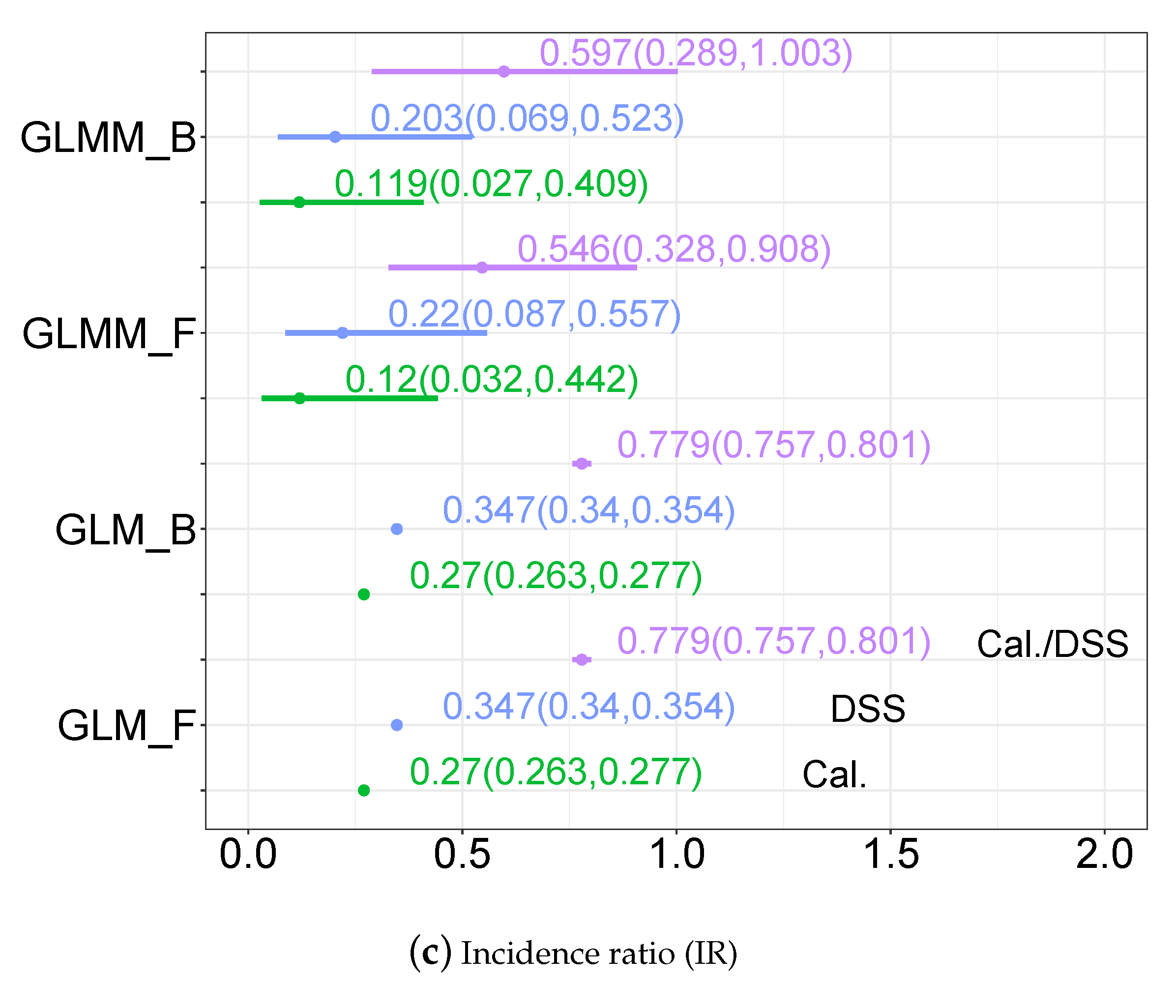
2.4.3. Incidence Ratio

Following the same strategy specified in the previous section for OR computation, IR for calendar (IR c a l ) and DSS (IR d s s )-based strategies against untreated control and IR for calendar against DSS were estimated for GLM_F model as follows:
IR ^ c a l = θ ^ c a l θ ^ 0 , IR ^ d s s = θ ^ d s s θ ^ 0 , IR ^ c a l / d s s = θ ^ c a l θ ^ d s s ,
Also for IR computation was carried out on a log scale and then log-transformed to convert them into the original metric [31]. Thus, based on the previous statement 95% confidence intervals were calculated according to
95 % CI IR ^ c a l = exp { log ( IR ^ c a l ) ± z 0.975 SE ( log ( IR ^ c a l ) } 95 % CI IR ^ d s s = exp { log ( IR ^ d s s ± z 0.975 SE ( log ( IR ^ d s s ) } 95 % CI IR ^ c a l / d s s = exp { log ( IR ^ c a l / d s s ± z 0.975 SE ( log ( IR ^ c a l / d s s ) }
in which z 0.975 denotes the 0.975 quantile of the normal distribution and SE the standard error.
For GLM_B, posterior distribution of the IRs was drawn from the transformation of posterior distribution of the model parameters involved and summarized by means of the median as a point estimate and the 95% credible intervals as a measure of uncertainty.
For GLMM_F model, average “experiment” IR for calendar and DSS-based strategy against the untreated control and IR for calendar against DSS were computed as follows:
IR ^ c a l M = θ ^ c a l M θ ^ 0 M , IR ^ d s s M = θ ^ d s s M θ ^ 0 M , IR ^ c a l M / d s s M = θ ^ c a l M θ ^ d s s M ,
but also in the log scale and with 95% confidence intervals were estimated in the same way as described in Equation (13) but adapting it to the parameters involved. For GLMM_B, posterior distributions of average IR were drawn from the transformation of posterior distribution of the model parameters concerned and summarised by means of the median as a point estimate and the 95% credible intervals as a measure of uncertainty.
IR c a l and IR d s s were used as a summary measure to quantify the efficacy of each fungicide program by means of relative changes in disease incidence. IR c a l / d s s was used to assess differences of calendar strategy in relation to DSS in terms of relative changes in disease incidence.

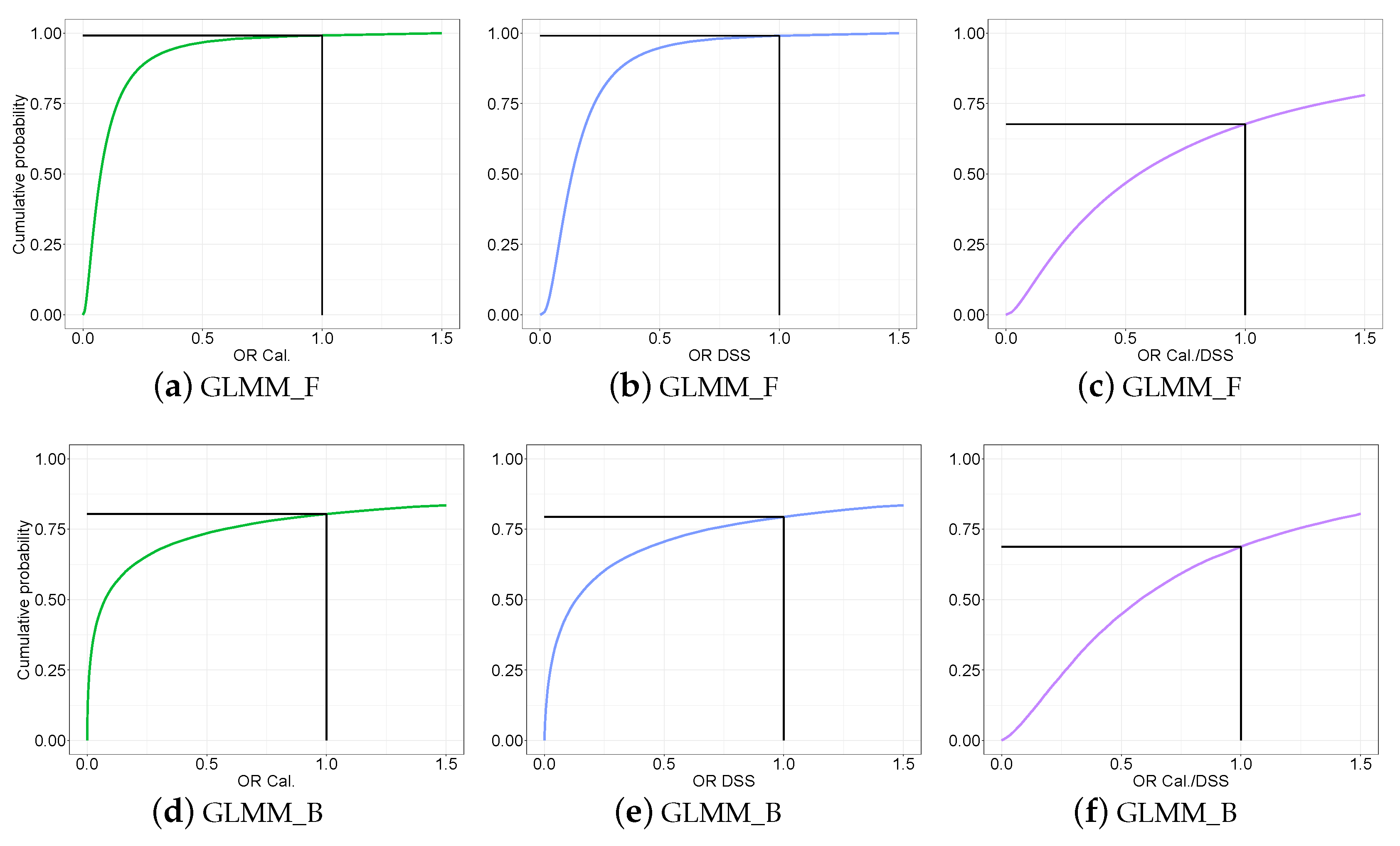
2.4.4. Predictive Distribution of the Odds Ratio

To assess the extent of the heterogeneity estimates among experiments, the uncertainty of the OR c a l , OR d s s and OR c a l / d s s were also re-evaluated by calculating their corresponding predictive distributions. These predictive distributions allow us to incorporate between-experiment variability and to derive the so-called prediction intervals. Following the computation strategy described in Section 2.4.2, predictive distributions of the OR were computed in log-scale and then back-transformed. Parameters involved here were γ cal , new and γ dss , new (they represent the values of γ cal ( i ) and γ cal ( i ) for a new experiment and new sub-experiments chosen at random). According to Higgins et al. [1], their corresponding predictive distribution were defined as
γ cal , new β ^ cal * σ ^ cal 2 + SE ( β ^ cal * ) 2 t N 2 γ dss , new β ^ dss * σ ^ dss 2 + SE ( β ^ dss * ) 2 t N 2
in which t N 2 denotes a t-distribution with N 2 degrees of freedom with N = 19 representing the number of experiments. With GLMM_B, the OR predictive distributions were derived from the predictive distributions of γ cal , new , γ dss , new . These distributions were obtained by sampling values of γ cal ( i ) and γ cal ( i ) from their corresponding posterior distributions using the following transformations, exp { γ cal , new } and exp { γ dss , new } .

3. Results

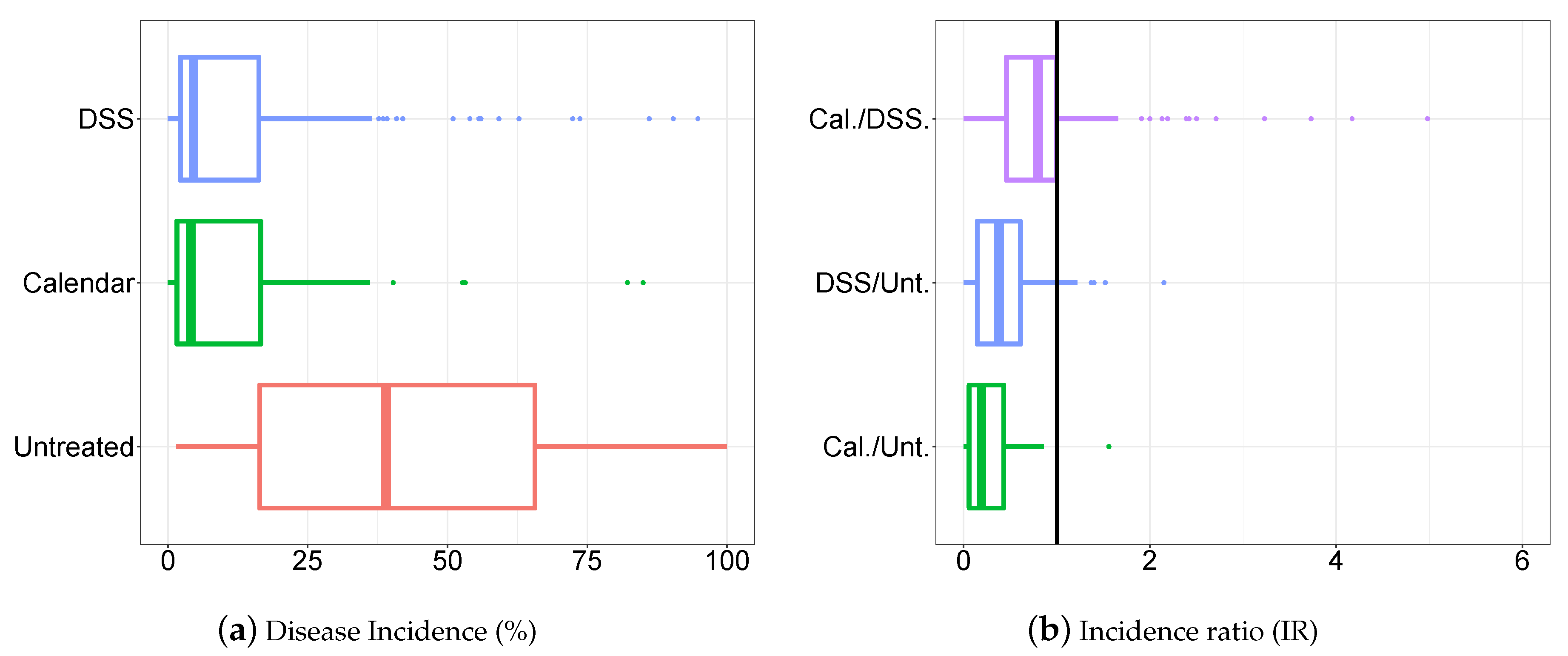
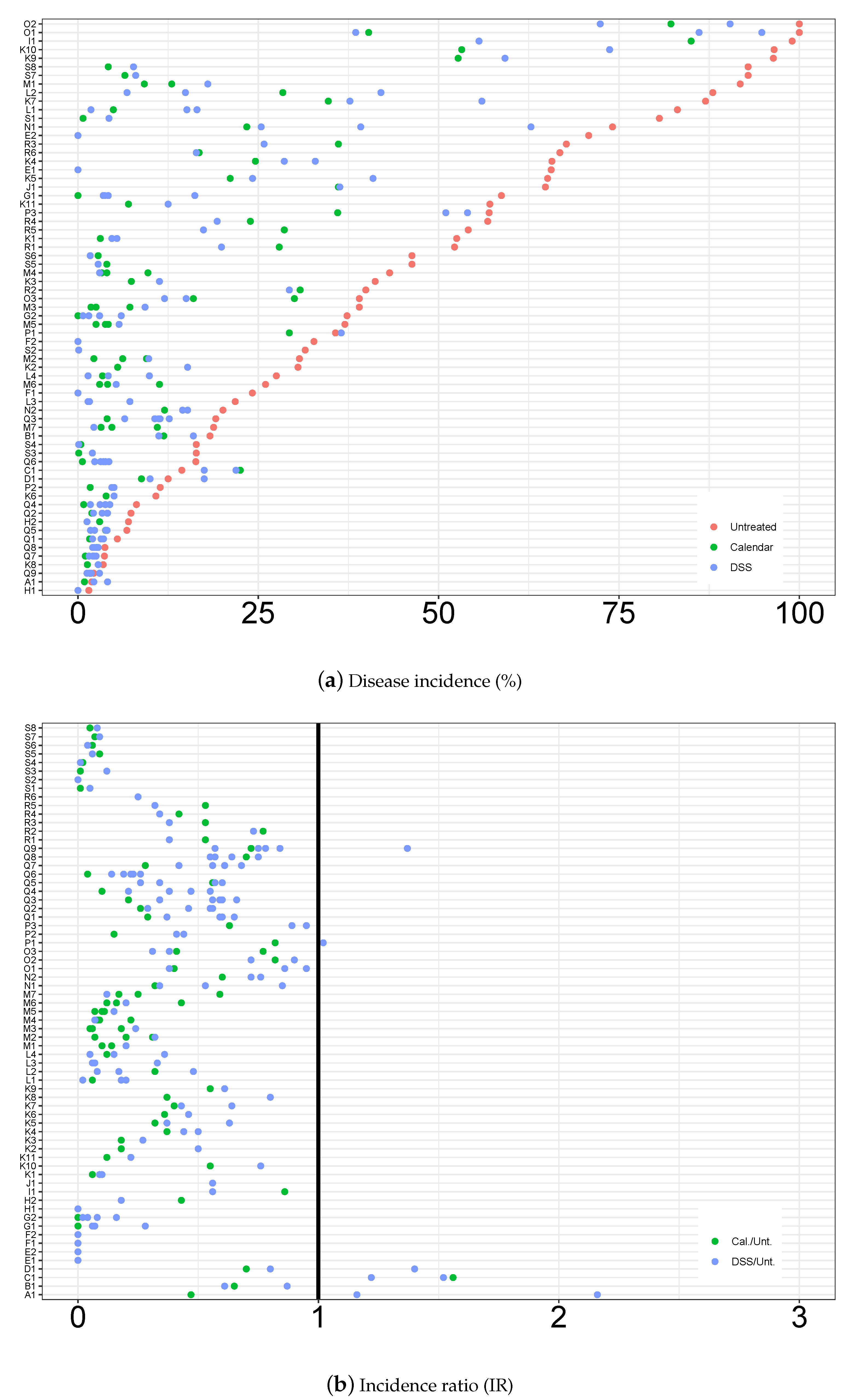
3.1. Descriptive Analysis of the Database

Disease incidence data are shown in Figure 1a and IRs for calendar and DSS strategies against the untreated control and for calendar against DSS in Figure 1b. Individual disease incidence data and IR values are shown in Figure 2a and Figure 2b, respectively. Note that some experiments show more than one IR (Cal./Unt. and DSS/Unt.) (Figure 2b) because more than one calendar and/or DSS strategies were evaluated (Table A3).
The disease incidence in untreated sub-experiments ranged from 1.5% to 100%. The mean and the median values were 43.17% and 39.00% (Figure 1a). The disease incidence for calendar and DSS-based strategies, showed overlapping distributions with similar mean (11.94% and 13.92%) and median (4.06% and 4.56%) values (Figure 1a). For Cal./Unt. and DSS/Unt. ratios the vast majority of observations were concentrated below the 1 with third quantile values ( Q 3 ) equal to 0.430 and 0.610 (Figure 1b, respectively, which shows a tested efficacy of both programs. Furthermore, both IR distributions overlap partially which reflects a similar efficacy between the two strategies ( Q 3 for Cal./DSS ratio was equal to 1).
Individual disease incidence under untreated sub-experiments presented in the vast majority of experiments higher values than their calendar and DSS counterparts, with only a few exceptions (A1, C1, D1, P1 and Q9) (Figure 2a). Calendar and their corresponding DSS showed similar disease incidence and IR values, sometimes higher for calendar, sometimes lower. Most IRs for Cal./Unt. and DSS/Unt. were lower than 1 with a few exceptions (A1, C1, D1, P1 and Q9 experiments) (Figure 2b).

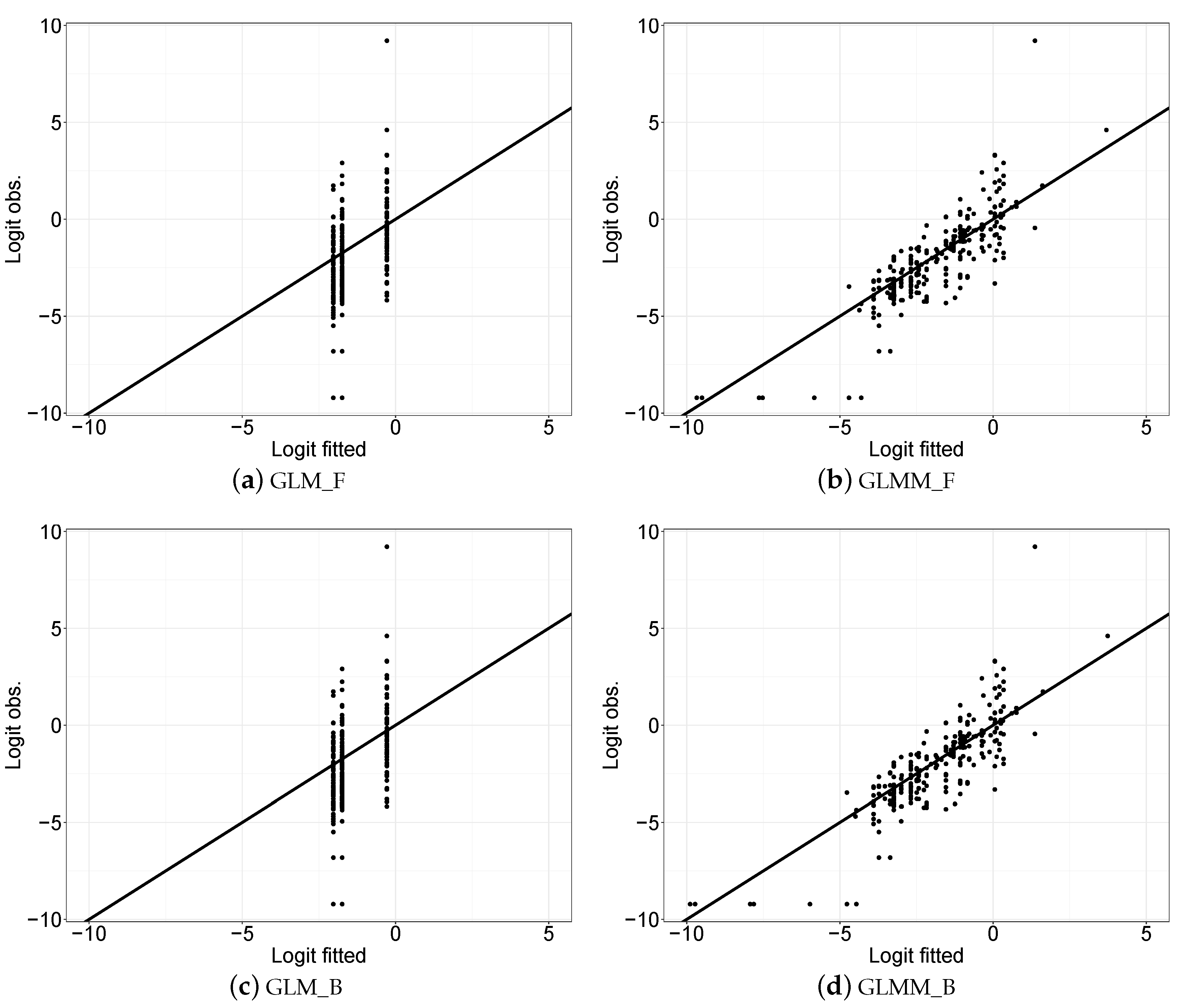
3.2. Statistical Modelling Evaluation

The “random-effects” models performed better than “fixed-effects” models with both frequentist and Bayesian approaches according to the AIC or DIC scores. AIC for models GLM_F and GLMM_F were estimated at 64189.00 and 26098.96 (Table 1). Their Bayesian counterparts (GLM_B and GLMM_B) got DIC scores of 64188.97 and 25860.42 (Table 2), respectively. Thus, with both inferential approaches, results were in favor of the GLMMs. This result was confirmed by the graphical analysis of logit(observed) vs. logit (estimated) of GLMs against GLMMs (Figure 3a,c and  Figure 3b,d) in which differences between observed and estimated (in logit scale) for GLMM were smaller. Figure 3a,c and  Figure 3b,d also showed that similar inferences were obtained between frequentist models and their Bayesian counterparts.

3.3. Statistical Modelling Inference Results

3.3.1. Parameter Estimates

Estimates for model parameters are shown in Table 1 (for frequentist, GLM_F and GLMM_F) and Table 2 (for Bayesian, GLM_B and GLMM_B). β 0 , β cal and β dss (for GLMs) and ( β 0 * , β cal * and β dss * ) (for GLMMs) had different point estimates. However, the signs of the coefficients were consistent between the GLM and GLMM. On the other hand, β 0 * , β cal * and β dss * showed wider confidence intervals (credible intervals) than β 0 , β cal and β dss . For the “random-effects” models (GLMM_F and GLMM_B), variance parameters ( σ 0 2 , σ cal 2 and σ dss 2 ) were far from 0 indicating a strong between-experiment  variability.

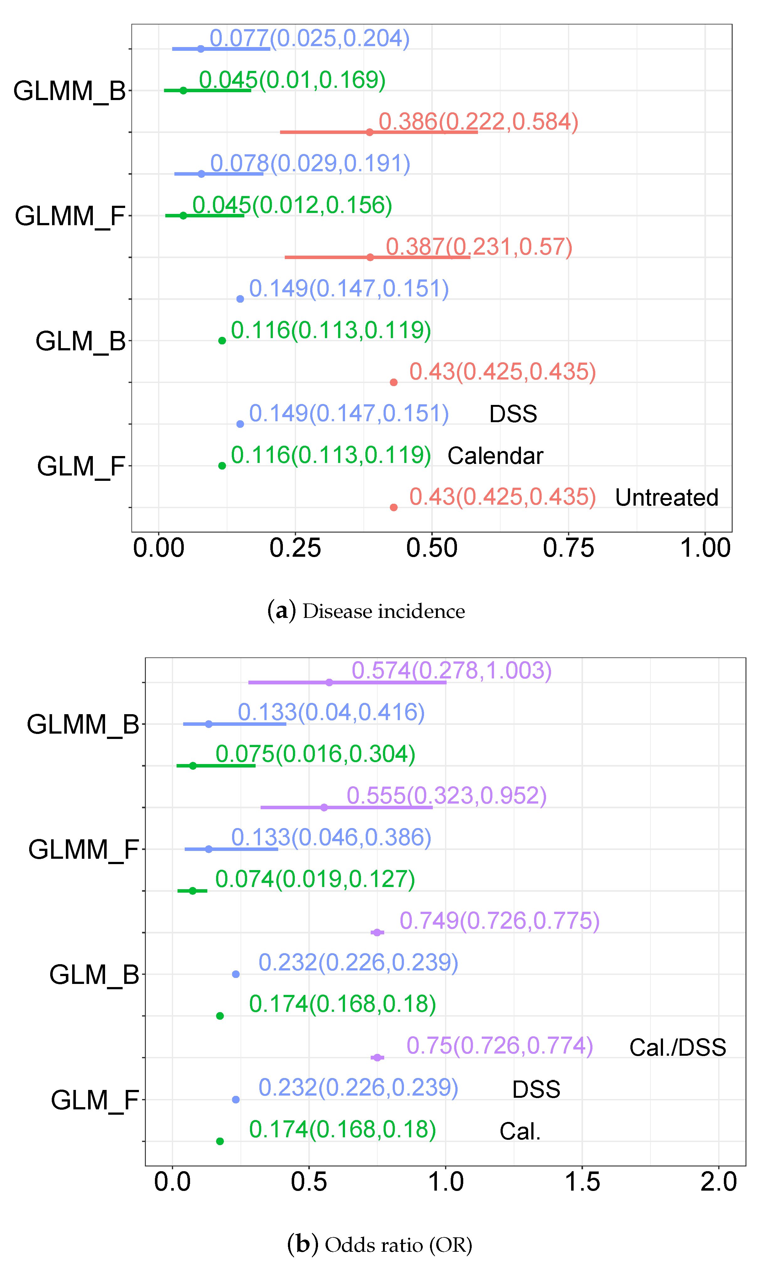
3.3.2. Disease Incidence, Odds Ratio and Incidence Ratio Estimates

Disease incidence, OR and IR estimates are displayed in Figure 4a–c for the four fitted models (GLM_F, GLM_B, GLMM_F and GLMM_B). Overall, all models showed similar point estimates. Confidence intervals obtained with the frequentist models were also similar to the credible intervals obtained with Bayesian models (GLM_F vs. GLM_B and GLMM_F vs. GLMM_B).
With the GLM_F, the estimated median disease incidence was higher for the untreated control, 0.43, than for calendar-based (0.116) and DDS-based strategies (0.149). The same trend was observed with the GLMM_F (median values of 0.387, 0.045, 0.078 for control, calendar and DDS strategies, respectively). GLMM_F revealed that the calendar and DDS estimates strongly overlap. Comparable results were obtained with the Bayesian models (GLM_B and GLMM_B).
With the GLM_F, OR median values for OR c a l , OR d s s , OR c a l / d s s were equal to 0.174, 0.232  and 0.750, respectively. With GLMM_F, these estimates were equal to 0.074, 0.133 and 0.55 (lower than frequentist estimates). Based on GLMM_F outputs, both calendar and DSS programs provide strong reduction of odds disease compared to the untreated controls (OR c a l and OR d s s < 1). Nevertheless, odds disease in calendar programs would be lower that in DSS (OR c a l / d s s < 1, but with some uncertainty). The level of reduction obtained with DSS is already very high and leads to low disease incidences (see Figure 4a). Similar results were obtained with the Bayesian models (GLM_B and GLMM_B) and also for the different modelling IR estimates (Figure 4c).

3.3.3. Predictive Distribution of the Odds Ratio

Figure 5 shows predictive distributions for the OR for the GLMM_F (Figure 5a–c) and GLMM_B (Figure 5d–f). The x-axis shows the possible values of the ORs and the y-axis the percentiles (%) of its corresponding predictive distribution. That is, for each specific value of the OR showed, its  corresponding cumulative probability denotes the % of chance to be less than this value.
Predictive distributions obtained with GLMM_F and with GLMM_B showed some noticeable differences for the OR c a l and OR d s s , not for the OR c a l / d s s . For GLMM_F, the probabilities (cumulative disease incidence probabilities) to have an OR lower than one are equal to 0.99 for both treatment strategies (Figure 5a,b). These results reveal that there is more than 99% to decrease the odds of disease with calendar and DSS strategies compared to untreated controls. However, according to the GLMM_B model, these probabilities were lower (about 0.8) (Figure 5d,e). Despite this difference, both models support that calendar and DSS strategies show high capabilities in reducing odds of disease. For both models, the probability that OR c a l / d s s was lower than one is equal to 0.68 which means that odds of disease might be lower with calendar but with a considerable degree of uncertainty (Figure 5c,f).

4. Discussion

In the present study, four statistical models were assessed to evaluate the sensitivity of a meta-analysis aimed to compare the efficacy of DSSs to the standard calendar-based fungicide strategies for the control of fungal diseases in crop plants. Statistical modelling was set comparing “fixed-effects” and “random-effects” models in the framework of GLMs with frequentist and Bayesian inferential methods. Our results showed that the different treatment effect measures considered (disease incidence, OR, and IR) are highly sensitive to the integration of random-effects which may lead to different conclusions. These differences between “fixed-effects” and “random-effects” models were reproduced in both inferential methods.
Our assessments based on AIC or DIC scores and the graphical analysis of discrepancies between observed and estimated values confirmed that the dataset was better described assuming variable treatment effects among the experiments. Conceptually, the inclusion of random treatment effects was in line with the intrinsic nature of the data, which were gathered from experiments carried out by researchers operating independently. Our analyses showed that variance parameters were higher than 1 (Table 1 and  Table 2), indicating a substantial heterogeneity among experiments [32,33].
Our results also indicated that the use of “fixed-effects” models may lead to a strong underestimation of the uncertainty associated with the treatment effects measures considered (incidence, OR, IR) to summarise treatment efficacies. For both GLMMs, fequentist and Bayesian, the  width of the uncertainty measures (confidence/credible intervals) was larger than in their GLM counterparts, due to the lack of correlation between sub-experiments observations that it is implicit in “fixed-effects” specification. Since all sub-experiments within an experiment were evaluated under the same local conditions, they cannot be considered independent. Thus, models ignoring this correlation (i.e., “fixed-effects”model), overestimate the number of independent data and thus underestimate the level of uncertainty as noted by Makowski et al. [5].
Models with “random-effects” allow deriving predictive distributions, which enable making more robust conclusions as indicated for the consideration of confidence/credible intervals, but  also by the prediction intervals [33]. This interesting feature was included in our work by the derivation of the predictive distribution for the OR. For both GLMMs, frequentist and Bayesian, the  estimation of treatment effects measures (disease incidence, OR, and IR) was obtained from the conditional median/posterior distribution (for Bayesian models) of the random experiment effect in which between-experiment variability for the different treatments was not considered. Predictive distributions allow the incorporation of these sources of variability and obtain a more appropriate treatment effect summary than the average [32]. Consequently, the use of predictions gained relevance in recent meta-analyses, becoming a standard statistical output due to its utility to assess heterogeneity and uncertainty of treatment effects in target populations [1,34,35]. According to the predictive distribution for the OR, both fungicide strategies showed to be equally effective in reducing disease incidence compared with the untreated control.
Frequentist and Bayesian models for both “fixed-effects” and “random-effects” produced almost identical results for disease incidence, OR and IR. Our results also highlighted the importance of properly interpret OR and IR as relative measures. These measures do not have an absolute interpretation and tend to be insensitive to differences in baseline events, so it could be recommendable to consider an absolute measure such as incidence estimates to support their interpretation. According  to  the previous studies of [5,32,36], our results confirmed that under a weakly informative prior scenario, frequentist  and Bayesian models perform similarly. However, this was not the case of the predictive distribution for the OR which slightly varied between the two methods, although they lead to the same conclusions. The problem of finding reasonably good methods for prediction in both frequentist and Bayesian methods is an open research field, thus it is necessary to check the performance of prediction methods in practical meta-analysis and to interpret them with caution.
Our results indicated that the both inferential methodologies evaluated had similar practical advantages, but each of them with its pros and its cons. In general, the Bayesian approach is conceptually more straightforward and addresses uncertainty in a more comprehensive and interpretable way. Posterior distributions (parameter or derived quantity) can be characterised in terms of probability. Thus, a 95% credible interval is simply the central portion of the posterior distribution that contains the 95% of parameter values. By contrast, frequentist inference does not allow probability statements about the parameters, the p-value is a measure of evidence against a null hypothesis when it is assumed to be true. Thus, a 95% confidence interval means that if the same procedure to construct confidence intervals was repeated many times, then in 95% of the cases the true value will lie within the interval.
The Bayesian approach also makes easier to extend simple models to more complex formulations [37]. Currently, there are several software alternatives available such as WinBUGS [38], JAGS [39], INLA [40], Stan [41], which allow implementing those complex models much easily than in the frequentist framework. By contrast, the requirement in the Bayesian context of setting a prior specification for each parameter could be a weakness in the inference process. In some non-informative prior scenarios, different prior specifications may lead to different posterior distributions affecting inference robustness [42]. Moreover, in some cases the computational demand of Bayesian models could be extremely intensive. Thus, as a general recommendation, inferential method choice in meta-analysis should address and balance all the issues above.
In the context of fungal diseases, DSS strategies allow growers to estimate the risk of disease and devise more efficient fungicide spray programs, integrating different sources of information for control decisions including action thresholds [11]. However, currently there is a limited degree of adoption of DSSs due in part to growers’ aversion to risks and a perceived lack of reliability of DSSs [13,43]. Building on numerous individual field trials conducted to evaluate DSSs in a wide range of disease-crop systems, our meta-analysis demonstrates that DSS-based programs are effective in reducing the incidence of fungal diseases with efficacy comparable to calendar-based fungicide programs. Statistical inference comparing the number of fungicide sprays in DSS-based and calendar-based strategies will be the topic of further research.

Author Contributions

Conceptualization, A.V.; methodology, E.L. and D.M.; database preparation, J.M.-M.; data analysis, E.L.; writing original draft, E.L.; review and editing, E.L., D.M., J.M.-M. and A.V. All authors have read and agreed to the published version of the manuscript.

Funding

This research was funded by INIA RTA2013-00004-C03-02 FEDER and INIA RTA2017-00009-C04-02 FEDER.

Acknowledgments

J.M.-M. would like to thank for the support by the Basque Government through the BERC 2018-2021 program and by the Ministry of Science, Innovation and Universities: BCAM Severo Ochoa accreditation SEV-2017-0718.

Conflicts of Interest

The authors declare no conflict of interest.

Abbreviations

The following abbreviations are used in this manuscript:
AICAkaike Information Criterion
DICDeviance Information Criterion
DSSDecision Support System
F&N TestsFungicide and Nematicide Tests
GLMGeneralized Linear Model
GLMMGeneralized Linear Mixed Model
IRIncidence Ratio
OROdds Ratio
SEStandard Error
WOSWeb of Science

Appendix A

Table A1. List of papers used in the meta-analysis, source and search string.
PaperSourceSearch String
Brown-Rytlewski et al. [44]F & N TestsForecasting
Brown-Rytlewski et al. [45]F & N TestsForecasting
Brown-Rytlewski et al. [46]F & N TestsForecasting
Brown-Rytlewski et al. [47]F & N TestsForecasting
Babadoost [48]F & N TestsWarning
Babadoost [49]F & N TestsWarning
Gleason et al. [50]F & N TestsWarning
Hovius and McDonald [51]F & N TestsForecasting
McDonald et al. [52]F & N TestsForecasting
Averre et al. [53]F & N TestsHard copies
Llorente et al. [54]WOSOther references
Bhatia et al. [55]WOSOther references
Byrne et al. [56]WOSOther references
Montesinos et al. [57]WOSOther references
Peres and Timmer [58]WOSOther references
Wu et al. [59]WOS(crop OR plant) AND disease AND (fungus OR fungi OR fungal OR fungicide)
AND (forecasting OR warning OR prediction OR predictive)
AND (decision-support OR decision OR support OR treatment OR model OR system)
AND (weekly OR calendar OR daily) AND (Comparison)
Louws et al. [60]WOS(crop OR plant) AND disease AND (fungus OR fungi OR fungal OR fungicide)
AND (forecasting OR warning OR prediction OR predictive)
AND (decision-support OR decision OR support OR treatment)
AND (weekly OR calendar OR daily) AND(model OR system)
Rasiukevivciute et al. [61]WOS(crop OR plant) AND disease AND (fungus OR fungi OR fungal OR fungicide)
AND (forecasting OR warning OR prediction OR predictive)
AND (decision-support OR decision OR support OR treatment)
AND(model OR system)
Rosli et al. [62]WOS(crop OR plant) AND (disease) AND (fungal OR fungi OR fun- gus)
AND (forecasting OR warning OR prediction) AND decision-support

Appendix B

Table A2. List of papers used in the meta-analysis. Papers are identified by its corresponding code  id. List of experiments used in the meta-analysis related to its corresponding paper. Experiments are characterised by an id and its corresponding location, crop type and disease *.
PaperExperiment
ReferenceIdLocationCropDisease *
Brown-Rytlewski et al. [44]A1Ohio, USWheatFusarium head blight
Brown-Rytlewski et al. [45]B1Michigan, USWheatFusarium head blight
Brown-Rytlewski et al. [46]C1Michigan, USWheatFusarium head blight
Brown-Rytlewski et al. [47]D1Michigan, USWheatFusarium head blight
Babadoost [48]E1California, USAppleSooty blotch complex
E2California, USAppleFlyspeck
Babadoost [49]F1California, USAppleSooty blotch complex
F2California, USAppleFlyspeck
Gleason et al. [50]G1Iowa, USAppleSooty blotch complex
G2Iowa, USAppleFlyspeck
Hovius and McDonald [51]H1Ontario, CALettuceDowny mildew
H2Ontario, CALettuceDowny mildew
Mcdonald et al. [52]I1Ontario, CALettuceDowny mildew
Averre et al. [53]J1North Carolina, USAsparagusCercospora blight
Llorente et al. [54]K1Emilia-Romagna, ITPearBrown spot
K2Girona, ESPearBrown spot
K3Emilia-Romagna, ITPearBrown spot
K4Girona, ESPearBrown spot
K5Girona, ESPearBrown spot
K6Emilia-Romagna, ITPearBrown spot
K7Girona, ESPearBrown spot
K8Girona, ESPearBrown spot
K9Girona, ESPearBrown spot
K10Girona, ESPearBrown spot
K11Emilia-Romagna, ITPearBrown spot
Bhatia et al. [55]L1Florida, USMandarinAlternaria brown spot
L2Florida, USMandarinAlternaria brown spot
L3Florida, USMandarinAlternaria brown spot
L4Florida, USMandarinAlternaria brown spot
Byrne et al. [56]M1Michigan, USTomatoAnthracnose
M2Michigan, USTomatoAnthracnose
M3Indiana, USTomatoAnthracnose
M4Michigan, USTomatoAnthracnose
M5Michigan, USTomatoAnthracnose
M6Indiana, USTomatoAnthracnose
M7Indiana, USTomatoAnthracnose
Montesinos et al. [57]N1Girona, ESPearBrown spot
N2Girona, ESPearBrown spot
Peres and Timmer [58]O1São Paulo, BRMandarinAlternaria brown spot
O2São Paulo, BRMandarinAlternaria brown spot
O3São Paulo, BRMandarinAlternaria brown spot
Wu et al. [59]P1California, USLettuceDowny mildew
P2California, USLettuceDowny mildew
P3California, USLettuceDowny mildew
Louws et al. [60]Q1Michigan, USTomatoEarly blight
Q2Michigan, USTomatoEarly blight
Q3Michigan, USTomatoEarly blight
Q4Michigan, USTomatoAnthracnose
Q5Michigan, USTomatoAnthracnose
Q6Michigan, USTomatoAnthracnose
Q7Michigan, USTomatoRhizoctonia fruit rot
Q8Michigan, USTomatoRhizoctonia fruit rot
Q9Michigan, USTomatoRhizoctonia fruit rot
Rasiukevivciute et al. [61]R1Kaunas, LTStrawberryGray mold
R2Kaunas, LTStrawberryGray mold
R3Kaunas, LTStrawberryGray mold
R4Kaunas, LTStrawberryGray mold
R5Kaunas, LTStrawberryGray mold
R6Kaunas, LTStrawberryGray mold
Rosli et al. [62]S1Iowa, USAppleSooty blotch complex /Flyspeck
S2Iowa, USAppleSooty blotch complex /Flyspeck
S3Iowa, USAppleSooty blotch complex /Flyspeck
S4Iowa, USAppleSooty blotch complex /Flyspeck
S5Iowa, USAppleSooty blotch complex /Flyspeck
S6Iowa, USAppleSooty blotch complex /Flyspeck
S7Iowa, USAppleSooty blotch complex /Flyspeck
S8Iowa, USAppleSooty blotch complex /Flyspeck
* APS (American Phytopathological Society) Common Names of Plant Diseases. https://www.apsnet.org/dcenter/resources/commonnames/Pages/default.aspx Accessed 08/03/20.
Table A3. List of papers used in the meta-analysis. Papers are identified by its corresponding reference and a code id. List of experiments used in the meta-analysis related to its corresponding paper. Experiments are characterised by an id and the number of sub-experiments for each fungicide strategy (untreated, calendar and DSS).
PaperExperimentSub-Experiments
ReferenceIdIdUntreatedCalendarDSS
Brown-Rytlewski et al. [44]AA1112
Brown-Rytlewski et al. [45]BB1112
Brown-Rytlewski et al. [46]CC1112
Brown-Rytlewski et al. [47]DD1112
Babadoost [48]EE1122
E2122
Babadoost [49]FF1122
F2122
Gleason et al. [50]GG1114
G2114
Hovius and McDonald [51]HH1111
H2111
McDonald et al. [52]II1111
Averre et al. [53]JJ1111
KK1112
K2111
K3111
K4112
K5112
Llorente et al. [54] K6111
K7112
K8111
K9111
K10111
K11111
Bhatia et al. [55]LL1113
L2113
L3113
L4113
MM1131
M2131
M3131
Byrne et al. [56] M4131
M5131
M6131
M7131
Montesinos et al. [57]NN1113
N2112
OO1113
Peres and Timmer [58] O2112
O3122
PP1111
Wu et al. [59] P2112
P3112
QQ1114
Q2114
Q3115
Q4114
Louws et al. [60] Q5114
Q6115
Q7114
Q8114
Q9115
Rasiukevivciute et al. [61]RR1111
R2111
R3111
R4111
R5111
R6111
Rosli et al. [62]SS1111
S2111
S3111
S4111
S5111
S6111
S7111
S8111
TOTAL 6786132

References

  1. Higgins, J.P.; Thompson, S.G.; Spiegelhalter, D.J. A re-evaluation of random-effects meta-analysis. J. R. Stat. Soc. A Stat. 2009, 172, 137–159. [Google Scholar] [CrossRef] [PubMed] [Green Version]
  2. Rosenberg, M.; Garrett, K.; Su, Z.; Bowden, R. Meta-analysis in plant pathology: synthesizing research results. Phytopathology 2004, 94, 1013–1017. [Google Scholar] [CrossRef] [PubMed] [Green Version]
  3. Ngugi, H.K.; Esker, P.D.; Scherm, H. Meta-analysis to determine the effects of plant disease management measures: review and case studies on soybean and apple. Phytopathology 2011, 101, 31–41. [Google Scholar] [CrossRef] [PubMed] [Green Version]
  4. Madden, L.; Paul, P. Meta-analysis for evidence synthesis in plant pathology: An overview. Phytopathology 2011, 101, 16–30. [Google Scholar] [CrossRef] [Green Version]
  5. Makowski, D.; Vicent, A.; Pautasso, M.; Stancanelli, G.; Rafoss, T. Comparison of statistical models in a meta-analysis of fungicide treatments for the control of citrus black spot caused by Phyllosticta citricarpa. Eur. J. Plant Pathol. 2014, 139, 79–94. [Google Scholar] [CrossRef]
  6. Sutton, A.J.; Abrams, K.R.; Jones, D.R.; Jones, D.R.; Sheldon, T.A.; Song, F. Methods for Meta-Analysis in Medical Research; John Wiley & Sons: Hoboken, NJ, USA, 2000; Volume 348. [Google Scholar]
  7. Philibert, A.; Loyce, C.; Makowski, D. Assessment of the quality of meta-analysis in agronomy. Agric. Ecosyst. Environ. 2012, 148, 72–82. [Google Scholar] [CrossRef]
  8. Borenstein, M.; Hedges, L.V.; Higgins, J.P.; Rothstein, H.R. Introduction to Meta-Analysis; John Wiley & Sons: Hoboken, NJ, USA, 2011. [Google Scholar]
  9. Rice, K.; Higgins, J.P.; Lumley, T. A re-evaluation of fixed effect (s) meta-analysis. J. R. Stat. Soc. A Stat. 2018, 181, 205–227. [Google Scholar] [CrossRef]
  10. McCullagh, P.; Nelder, J. Generalized Linear Models, 2nd ed.; Chapman and Hall/CRC Monographs on Statistics and Applied Probability Series; Chapman & Hall: Boca Raton, FL, USA, 1989. [Google Scholar]
  11. Magarey, R.; Travis, J.; Russo, J.; Seem, R.; Magarey, P. Decision support systems: Quenching the thirst. Plant Dis. 2002, 86, 4–14. [Google Scholar] [CrossRef] [Green Version]
  12. De Wolf, E.D.; Isard, S.A. Disease cycle approach to plant disease prediction. Annu. Rev. Phytopathol. 2007, 45, 203–220. [Google Scholar] [CrossRef]
  13. Shtienberg, D. Will decision-support systems be widely used for the management of plant diseases? Annu. Rev. Phytopathol. 2013, 51, 1–16. [Google Scholar] [CrossRef]
  14. Warn, D.E.; Thompson, S.; Spiegelhalter, D.J. Bayesian random effects meta-analysis of trials with binary outcomes: methods for the absolute risk difference and relative risk scales. Stat. Med. 2002, 21, 1601–1623. [Google Scholar] [CrossRef] [PubMed]
  15. Jackson, D.; White, I.R. When should meta-analysis avoid making hidden normality assumptions? Biom. J. 2018, 60, 1040–1058. [Google Scholar] [CrossRef] [PubMed] [Green Version]
  16. Hoyer, A.; Kuss, O. Meta-analysis for the comparison of two diagnostic tests to a common gold standard: A generalized linear mixed model approach. Stat. Methods Med. Res. 2018, 27, 1410–1421. [Google Scholar] [CrossRef] [PubMed]
  17. Bates, D.; Mächler, M.; Bolker, B.; Walker, S. Fitting linear mixed-effects models using lme4. J. Stat. Softw. 2015, 67, 1–48. [Google Scholar] [CrossRef]
  18. R Core Team. R: A Language and Environment for Statistical Computing; R Foundation for Statistical Computing: Vienna, Austria, 2018. [Google Scholar]
  19. Sakamoto, Y.; Ishiguro, M.; Kitagawa, G. Akaike Information Criterion Statistics; Taylor & Francis: Abingdon, UK, 1986. [Google Scholar]
  20. Burnham, K.P.; Anderson, D.R. Multimodel inference: Understanding AIC and BIC in model selection. Sociol. Method. Res. 2004, 33, 261–304. [Google Scholar] [CrossRef]
  21. Lázaro, E.; Armero, C.; Roselló, J.; Serra, J.; Muñoz, M.; Canet, R.; Galipienso, L.; Rubio, L. Comparison of viral infection risk between organic and conventional crops of tomato in Spain. Eur. J. Plant Pathol. 2019, 155, 1145–1154. [Google Scholar] [CrossRef]
  22. Chen, M.H.; Shao, Q.M. Monte Carlo estimation of Bayesian credible and HPD intervals. J. Comput. Graph. Stat. 1999, 8, 69–92. [Google Scholar]
  23. Gelman, A.; Jakulin, A.; Pittau, M.G.; Su, Y.S. A weakly informative default prior distribution for logistic and other regression models. Ann. Appl. Stat. 2008, 2, 1360–1383. [Google Scholar] [CrossRef]
  24. Su, Y.S.; Yajima, M. R2jags: Using R to run ‘JAGS’. R package version 0.5-7 2015, 34. Available online: https://cran.r-project.org/web/packages/R2jags/index.html (accessed on 10 March 2020).
  25. Gelman, A.; Rubin, D.B. Inference from iterative simulation using multiple sequences. Stat. Sci. 1992, 7, 457–472. [Google Scholar] [CrossRef]
  26. Spiegelhalter, D.J.; Best, N.G.; Carlin, B.P.; Van Der Linde, A. The deviance information criterion: 12 years on. J. R. Stat. Soc. B Met. 2014, 76, 485–493. [Google Scholar] [CrossRef]
  27. Carlin, B.P.; Louis, T.A. Bayesian Methods for Data Analysis; Chapman and Hall/CRC: Boca Raton, FL, USA, 2008. [Google Scholar]
  28. Engels, E.A.; Schmid, C.H.; Terrin, N.; Olkin, I.; Lau, J. Heterogeneity and statistical significance in meta-analysis: an empirical study of 125 meta-analyses. Stat. Med. 2000, 19, 1707–1728. [Google Scholar] [CrossRef]
  29. Deeks, J.J. Issues in the selection of a summary statistic for meta-analysis of clinical trials with binary outcomes. Stat. Med. 2002, 21, 1575–1600. [Google Scholar] [CrossRef] [PubMed]
  30. Held, L.; Bové, D.S. Frequentist Properties of the Likelihood. In Applied Statistical Inference; Springer: Berlin/Heidelberg, Germany, 2014; pp. 79–122. [Google Scholar]
  31. Schwarzer, G.; Carpenter, J.R.; Rücker, G. Meta-Analysis with Binary Outcomes. In Meta-Analysis with R; Springer: Berlin/Heidelberg, Germany, 2015; pp. 55–83. [Google Scholar]
  32. Spiegelhalter, D.J.; Abrams, K.R.; Myles, J.P. Bayesian Approaches to Clinical Trials and Health-Care Evaluation; John Wiley & Sons: Hoboken, NJ, USA, 2004; Volume 13. [Google Scholar]
  33. Graham, P.L.; Moran, J.L. Robust meta-analytic conclusions mandate the provision of prediction intervals in meta-analysis summaries. J. Clin. Epidemiol. 2012, 65, 503–510. [Google Scholar] [CrossRef]
  34. Riley, R.D.; Higgins, J.P.; Deeks, J.J. Interpretation of random effects meta-analyses. BMJ 2011, 342, d549. [Google Scholar] [CrossRef] [Green Version]
  35. Hamaguchi, Y.; Noma, H.; Nagashima, K.; Yamada, T.; Furukawa, T.A. Frequentist performances of Bayesian prediction intervals for random-effects meta-analysis. arXiv 2019, arXiv:1907.00345. [Google Scholar]
  36. Gelman, A.; Carlin, J.B.; Stern, H.S.; Dunson, D.B.; Vehtari, A.; Rubin, D.B. Bayesian Data Analysis; Chapman and Hall/CRC: Boca Raton, FL, USA, 2013. [Google Scholar]
  37. Hong, H.; Carlin, B.P.; Shamliyan, T.A.; Wyman, J.F.; Ramakrishnan, R.; Sainfort, F.; Kane, R.L. Comparing Bayesian and frequentist approaches for multiple outcome mixed treatment comparisons. Med. Decis. Mak. 2013, 33, 702–714. [Google Scholar] [CrossRef]
  38. Ntzoufras, I. Bayesian Modeling Using WinBUGS; John Wiley & Sons: Hoboken, NJ, USA, 2011; Volume 698. [Google Scholar]
  39. Plummer, M. Rjags: Bayesian Graphical Models using MCMC. R package version 4-6 2016. Available online: https://www.rdocumentation.org/packages/rjags/versions/4-6 (accessed on 10 March 2020).
  40. Rue, H.; Riebler, A.; Sørbye, S.H.; Illian, J.B.; Simpson, D.P.; Lindgren, F.K. Bayesian computing with INLA: A review. Annu. Rev. Stat. Appl. 2017, 4, 395–421. [Google Scholar] [CrossRef] [Green Version]
  41. Bürkner, P.C. brms: An R package for Bayesian multilevel models using Stan. J. Stat. Softw. 2017, 80, 1–28. [Google Scholar] [CrossRef] [Green Version]
  42. Lázaro, E.; Armero, C.; Rubio, L. Bayesian correlated models for assessing the prevalence of viruses in organic and non-organic agroecosystems. SORT-Stat. Oper. Res. T. 2017, 1, 93–116. [Google Scholar]
  43. Gent, D.H.; De Wolf, E.; Pethybridge, S.J. Perceptions of risk, risk aversion, and barriers to adoption of decision support systems and integrated pest management: an introduction. Phytopathology 2011, 101, 640–643. [Google Scholar] [CrossRef] [Green Version]
  44. Brown-Rytlewski, W.W.; Schafer, R.; Berry, D. Evaluation of fungicides for control of Fusarium head scab of winter wheat at Sandusky, MI, 2006. Plant Dis. Manag. Rep. 2007, 1, CF017. [Google Scholar]
  45. Brown-Rytlewski, W.W.; Schafer, R.; Berry, D. Evaluation of fungicides for control of Fusarium head scab of winter wheat at Williamston MI, 2006. Plant Dis. Manag. Rep. 2007, 1, CF016. [Google Scholar]
  46. Brown-Rytlewski, W.W.; Schafer, R.; Berry, D. Evaluation of fungicides for control of Fusarium head scab of winter wheat at East Lansing, MI, 2006. Plant Dis. Manag. Rep. 2007, 1, CF018. [Google Scholar]
  47. Brown-Rytlewski, W.W.; Schafer, R.; Berry, D. Evaluation of fungicides for control of Fusarium head scab of winter wheat at Saginaw, MI, 2006. Plant Dis. Manag. Rep. 2007, 1, CF019. [Google Scholar]
  48. Babadoost, M. Performance of reduced-risk fungicides and a wetness-based warning system for control of sooty blotch and flyspeck of apple, 2006. Plant Dis. Manag. Rep. 2007, 1, PF001. [Google Scholar]
  49. Babadoost, M. Evaluating effectiveness of reduced-risk fungicides and a wetness-based warning system for control of sooty blotch and flyspeck of apple, 2007. Plant Dis. Manag. Rep. 2008, 1, PF050. [Google Scholar]
  50. Gleason, M.L.; Massman, J.M.; Sisson, A.J.; Mueller, T.A.; S, M.D. Evaluation of fungicides sprayed according to different disease warning systems for control of sooty blotch and flyspeck, 2004. Fungic. Nematic. Tests 2005, 60, PF020. [Google Scholar]
  51. Hovius, M.H.Y.; McDonald, M.R. Field evaluation of forecasting systems to optimize fungicide applications for downy mildew of lettuce. Fungic. Nematic. Tests 2000, 54, 146–147. [Google Scholar]
  52. McDonald, M.R.; Vander-Kooi, L.; Roberts, L. Field evaluation of Bremcast: a forecasting system for downy mildew of lettuce. Fungic. Nematic. Tests 2001, 56, V21. [Google Scholar]
  53. Averre, C.W.; Jenkins, S.F.; Cooperman, C. Evaluation of various spray schedules for control of Cercospora leaf spot on asparagus, 1983. Fungic. Nematic. Tests 1984, 39, 103. [Google Scholar]
  54. Llorente, I.; Vilardell, P.; Bugiani, R.; Gherardi, I.; Montesinos, E. Evaluation of BSPcast disease warning system in reduced fungicide use programs for management of brown spot of pear. Plant Dis. 2000, 84, 631–637. [Google Scholar] [CrossRef] [PubMed] [Green Version]
  55. Bhatia, A.; Roberts, P.; Timmer, L. Evaluation of the Alter-Rater model for timing of fungicide applications for control of Alternaria brown spot of citrus. Plant Dis. 2003, 87, 1089–1093. [Google Scholar] [CrossRef] [PubMed] [Green Version]
  56. Byrne, J.; Hausbeck, M.; Latin, R. Efficacy and economics of management strategies to control anthracnose fruit rot in processing tomatoes in the Midwest. Plant Dis. 1997, 81, 1167–1172. [Google Scholar] [CrossRef] [Green Version]
  57. Montesinos, E.; Vilardell, P. Evaluation of FAST as a forecasting system for scheduling fungicide sprays for control of Stemphylium vesicarium on pear. Plant Dis. 1992, 76, 1221–1226. [Google Scholar] [CrossRef]
  58. Peres, N.; Timmer, L. Evaluation of the Alter-Rater model for spray timing for control of Alternaria brown spot on Murcott tangor in Brazil. Crop Prot. 2006, 25, 454–460. [Google Scholar] [CrossRef]
  59. Wu, B.; Subbarao, K.; Van Bruggen, A.; Koike, S. Comparison of three fungicide spray advisories for lettuce downy mildew. Plant Dis. 2001, 85, 895–900. [Google Scholar] [CrossRef] [Green Version]
  60. Louws, F.J.; Hausbeck, M.K.; Stephens, C. Impact of reduced fungicide and tillage on foliar blight, fruit rot, and yield of processing tomatoes. Plant Dis. 1996, 80, 1251–1256. [Google Scholar] [CrossRef]
  61. Rasiukevičiūtė, N.; Uselis, N.; Valiuškaitė, A. The use of forecasting model iMETOS® for strawberry grey mould management. Zemdirbyste 2019, 106, 143–150. [Google Scholar] [CrossRef]
  62. Rosli, H.; Mayfield, D.A.; Batzer, J.C.; Dixon, P.M.; Zhang, W.; Gleason, M.L. Evaluating the performance of a relative humidity-based warning system for sooty blotch and flyspeck in Iowa. Plant Dis. 2017, 101, 1721–1728. [Google Scholar] [CrossRef] [PubMed] [Green Version]
Figure 1. Overall distribution of: (a) Disease incidence for DSS, calendar-based strategies and untreated; and (b) incidence ratios for Cal./DSS, DSS/Unt. and Cal./Unt..
Agronomy 10 00560 g001
Figure 2. (a) Individual disease incidence for sub-experiments under untreated, calendar and DSS-based strategies; and (b) individual Incidence Ratio for Cal./Unt. and DSS/Unt. Each letter encodes a paper and each letter/number encodes an experiment. Each row displays individual values for each sub-experiment.
Agronomy 10 00560 g002
Figure 3. Comparison of logit(observed disease incidence) vs. logit(fitted disease incidence) for: (a) GLM_F; (b) GLMM_F; (c) GLM_B; and, (d) GLMM_B. In solid black line, regression line 1:1.
Agronomy 10 00560 g003
Figure 4. Comparison of estimated values of disease incidence, odds ratios and incidence ratios obtained with the four fitted models. (a) Disease incidence for DSS (blue), calendar (green) and untreated (pink) treatments; (b) odds ratio for calendar/DSS (purple), DSS/untreated (blue) and calendar/untreated (green); and (c) incidence ratio for calendar/DSS (purple), DSS/untreated (blue) and calendar/untreated (green).
Agronomy 10 00560 g004aAgronomy 10 00560 g004b
Figure 5. Predictive distribution of odds ratio for calendar-based strategy against untreated control computed with (a) GLMM_F and (d) GLMM_B. Predictive distribution of odds ratio for DSS-based strategy against the untreated control computed with (b) GLMM_F and, (e) GLMM_B. Predictive distribution of odds ratio for calendar-based strategy against DSS-based strategy computed with (c) GLMM_F and, (f) GLMM_B. The solid black line indicates the % percentile which matches with an odds ratio lower than 1.
Agronomy 10 00560 g005
Table 1. Parameter estimates, standard error and 95% confidence intervals for GLM_F and GLMM_F.
GLM_FGLMM_F
β 0 0.282 * ( 0.302 , 0.262 ) β 0 * 0.461 ( 1.205 , 0.282 )
β cal 1.748 * ( 1.781 ; 1.714 ) β cal * 2.604 * ( 3.944 , 1.264 )
β dss 1.460 * ( 1.487 , 1.433 ) β dss * 2.014 * ( 3.077 ; 0.951 )
σ 0 2 2.677
σ cal 2 8.369
σ dss 2 5.387
σ 0 , cal −1.066
σ 0 , dss −1.453
σ cal , dss 6.387
AIC64,189.000 26,098.962
* 0 outside the confidence interval.
Table 2. Median of the posterior distribution and 95% credible intervals for GLM_B and GLMM_B.
GLM_BGLMM_B
β 0 0.282 * ( 0.302 , 0.262 ) β 0 * 0.462 ( 1.252 , 0.337 )
β cal 1.748 * ( 1.781 ; 1.714 ) β cal * 2.585 * ( 4.131 , 1.189 )
β dss 1.459 * ( 1.486 , 1.432 ) β dss * 2.017 * ( 3.222 ; 0.877 )
σ 0 2 2.778 ( 1.453 , 6.057 )
σ cal 2 8.717 ( 3.961 , 22.126 )
σ dss 2 5.726 ( 2.849 , 13.340 )
σ 0 , cal −1.061 ( 4.512 , 1.301 )
σ 0 , dss −1.433 ( 4.562 , 0.292 )
σ cal , dss 6.614 ( 3.167 , 15.701 )
DIC64,188.970 25,860.42
* 0 outside the credible interval.

