Abstract
Although the use of biocontrol agents (BCAs) to manage plant pathogens has emerged as a sustainable means for disease control, global reliance on their use remains relatively insignificant and the factors influencing their efficacy remain unclear. In this work, we further developed an existing generic model for biocontrol of foliar diseases, and we parametrized the model for the Botrytis cinerea–grapevine pathosystem. The model was operated under three climate types to study the combined effects on BCA efficacy of four factors: (i) BCA mechanism of action, (ii) timing of BCA application with respect to timing of pathogen infection (preventative vs. curative), (iii) temperature and moisture requirements for BCA growth, and (iv) BCA survival capability. All four factors affected biocontrol efficacy, but factors iii and iv accounted for > 90% of the variation in model simulations. In other words, the most important factors affecting BCA efficacy were those related to environmental conditions. These findings indicate that the environmental responses of BCAs should be considered during their selection, BCA survival capability should be considered during both selection and formulation, and weather conditions and forecasts should be considered at the time of BCA application in the field.
1. Introduction
Biocontrol of plant pathogens has emerged as a sustainable method of disease management and as a viable way to reduce the application of chemicals in agriculture [1,2,3,4]. The reasons for increasing restrictions on the use of chemicals and for increasing interest in biocontrol include the negative effects of chemicals on human health and the environment [5,6], pathogen-acquired resistance to commonly applied chemicals, and the lack of replacement products [7]. Biocontrol involves the use of fungi, bacteria, yeasts, or viruses (together referred to as biocontrol agents or BCAs) that may suppress plant pathogens via competition for nutrients or space, antibiosis, parasitism, and induced host plant resistance [1].
Despite the extensive research on biocontrol and the potential of using BCAs as alternatives to chemicals, the global reliance on BCA use remains relatively insignificant [4]. Many BCAs have been reported to suppress plant pathogens under controlled conditions in laboratories and greenhouses, but only a few have performed consistently in the field [8,9]. A possible reason for the lack of success of BCAs in the field is that they are often used in a similar manner as fungicides, even though the processes influencing the efficacy of BCAs are complex [10]. The complexity is not surprising, because BCAs are living organisms that dynamically interact with the target pathogen, the host plant, the microbial communities in the phyllosphere, and the physical environment [11]. Fluctuating environmental conditions in the field influence BCA survival, establishment, growth, and activity [1,12,13]. Although temperature and humidity have been evaluated as key factors affecting BCA efficacy in some studies [11,12,14,15,16,17,18], the complex relationships between BCAs and the environment remain difficult to predict and manage [19,20].
Mathematical models have been used to study disease epidemics in relation to BCA dynamics. Some models focus on the relationship between BCA dose and pathogen infection [21,22,23,24], while others consider more complex interactions [25,26,27]. Jeger et al. [28] developed a mean-field deterministic model that is able to predict the likelihood of the successful control of foliar diseases by a single BCA in relation to the biocontrol mechanisms involved. The latter model is a standard susceptible-infected-removed (SIR) model, in which host–pathogen dynamics are coupled with pathogen–BCA dynamics through four biocontrol mechanisms: mycoparasitism, competition, antibiosis, and induced plant host resistance. Improved versions of this model were subsequently proposed to compare the effects of using a single BCA with two biocontrol mechanisms [29] vs. the combined use of two BCAs, each with an individual mechanism [30], or the effects of constant vs. fluctuating temperatures on biocontrol efficacy [31]. The latter study revealed that the dynamics of biocontrol differed greatly under constant vs. fluctuating temperatures and stressed the importance of characterizing biocontrol activity in relation to environmental conditions and disease development.
In the current research, we enlarged the model proposed by Jeger et al. [28] by including (i) the effects of environmental conditions on the interactions between the pathogen and BCA and (ii) the dynamics of host growth and senescence. The proposed model structure is generic and could be applied to various pathosystems and several pathogen–BCA interactions. We also parametrized the model for the Botrytis cinerea–grapevine pathosystem. Botrytis cinerea is the causal agent of Botrytis bunch rot (BBR), a serious disease that damages all grapevine organs, and especially bunches, resulting in substantial losses of quantity and quality [32,33,34]. We then operated the model under three climate types to determine whether the use of a specific BCA is more likely to result in effective biocontrol of B. cinerea depending on its adaptation to fluctuating conditions of temperature and relative humidity. In the following sections, we describe the model, its parametrization for the BBR case-study (i.e., Botrytis bunch rot in grapes caused by Botrytis cinerea), and (iii) model simulations for different BCAs under different climate types.
2. Model Description
The model is based on the generic model developed by Jeger et al. [28] and further revised by Xu et al. [29]. In this model, a classic susceptible-infected-removed (SIR) model for host–pathogen dynamics [35] is combined with a model for pathogen–BCA dynamics. The modified model was developed by using a system dynamics approach [36], in which the system (consisting of the plant, the pathogen, the BCA, and the environment) is described by state variables, which represent plant tissue categories in relation to the pathogen–BCA interaction. The system moves from one state variable to another by mean of fluxes, which are regulated by rate variables (or rates). Rates depend on the characteristics of the pathogen, host plant, and BCA and may also be influenced by the weather conditions that affect the processes underlying the dynamics of both the pathogen (i.e., infection and infectiousness) and the BCA (i.e., growth and survival capability). The effect of external variables on processes is accounted for by driving functions (i.e., temperature, relative humidity, and moisture duration).
The model is generic and can be operated for fungal pathogens of aerial plant parts (e.g., leaves and fruits) and for BCAs with different mechanisms of action (MOA), including competition with the pathogen for space and nutrients, direct activity on the pathogen through antibiosis or mycoparasitism, and induced resistance in the plant. These are the main MOA of the currently used BCAs [1]. The model works with a time step of 1 day.
The model was developed by using the software STELLA® (abbreviation of Systems Thinking, Experimental Learning Laboratory with Animation, 1.6.1. version, Isee Systems, Lebanon, NH 03766 USA [37]), a visual programming language for system dynamics modelling. The model was diagrammed (Figure 1) by using the graphic representation of Forrester [38], which combines state variables (rectangles), flows (solid arrows), rates (valves), parameters and coefficients (circles), and numerical relationships (dashed arrows). Acronyms for state variables, rates, driving variables, and parameters are explained in Table 1.
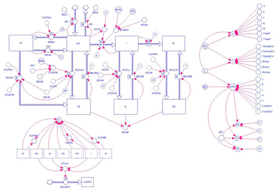
Figure 1.
Model flowchart in which the state variables are host tissue categories that change according to the interactions among the pathogen, biocontrol agents (BCAs), and the environment. The diagram uses the symbols developed by Forrester [38]. The core of the model is based on a classic susceptible-infected-removed (SIR) model, with tissue evolving from healthy-susceptible (HS) to infectious (I) and removed (R). The rate of infection of tissue (RI) depends on primary (STARTP) and secondary infections (I). The rate of resistance induction by a BCA (RRES) depends on BCA application (STARTB) and the total amount of healthy-susceptible tissue (HS). The rates of BCA colonization (RCOLH, RCOLI, RCOLR, and RCOLHr) depend on BCA application (STARTB) and the total amount of colonized tissue (BSUM). The structure incorporates host growth (RG) and physiological senescence (RS). Symbols for state variables, rates, and parameters are explained in Table 1.

Table 1.
List of state variables, rates, driving variables, and parameters used in the model.
2.1. State Variables and Connecting Flows
The site of the system consists of K units of plant tissue that can be potentially occupied (i.e., affected) by the pathogen during the epidemic. The K units represent the state variables of the model and belong to one of the following non-overlapping categories of tissue: (i) healthy and susceptible to infection (HS); (ii) affected by the pathogen and infectious, i.e., can generate new, secondary infections (I); (iii) affected by the pathogen and removed, i.e., no longer infectious (R); (iv) healthy and colonized by the BCA, i.e., resistant to infection by the pathogen (Hr); (v) healthy and colonized by the BCA, i.e., which is protected from the pathogen (Hb); (vi) infectious and colonized by the BCA, i.e., unable to generate new infections (Ib); and (vii) removed and colonized by the BCA (Rb). The seven state variables are mutually exclusive so that:
K = HS + I + R + Hr + Hb + Ib + Rb.
The model considers that, during the epidemic and as a consequence of BCA application, the K units move from one state variable to another by means of rates.
At the beginning of a simulation, all of the plant tissue is in the state variable HS. The size of HS is dynamic and increases over time as a consequence of plant growth (in such a way that HS = 1 at the time of maximum plant size) or decreases as a consequence of senescence (which is relevant for those diseases in which the senescent plant tissue is no longer susceptible to infection). Inflow (rate of growth, RG) and outflow (rate of senescence, RS) of host tissue with respect to HS is calculated as follows:
in which t is the current day, t−1 is the day before, and RRGt and RRSt are relative rates of host growth and senescence on day t, respectively.
RGt = HSt−1 × RRGt
RSt = HSt−1 × RRSt
The host tissue in the state variable HS moves to state variable I as a consequence of infection by the pathogen; this flow is regulated by RI, the rate of infection, which is calculated as follows:
in which STARTP is the initial inflow of the pathogen into the system, b is the relative rate of infection, I is as previously defined, and COFR is the correction factor for occupied tissue.
RIt = STARTPt + bt × It−1 × COFRt
In Equation (4), STARTP is calculated by assuming that the pathogen enters the system starting on day PIN (the day of the first seasonal infection) and continues to enter at a constant rate RPIN for a period of PDUR days; PIN, RPIN, and PDUR are all model parameters that are defined for each situation.
In Equation (4), COFR is calculated as follows:
in which K and HS are as previously defined.
COFRt = (1 − ((Kt − HSt)/Kt)
The host tissue in the state variable I moves to state variable R when the infectious period (i.e., the period during which the pathogen continues producing inoculum on affected tissue) is over; this outflow is regulated by RR, the rate of removal, which is calculated as follows:
in which h is the relative rate of removal and I is as previously defined.
RRt = ht × It−1
The model considers that, at any time during the simulation period, a BCA enters the system because of human intervention (i.e., a treatment with the BCA); this can be before, at the same time as, or after the pathogen. The BCA inflow is regulated by STARTB, which is calculated for a period of BDUR days (i.e., the period during which the BCA is applied), starting from day BIN (i.e., the day on which the BCA is applied) at a constant rate equal to RBIN; BIN, RBIN, and BDUR are all model parameters that are defined for each situation.
The introduction of the BCA generates outflows from HS, so that the healthy tissue cannot be infected by the pathogen and, therefore, cannot move to I. The model considers that this outflow can be caused by BCAs that induce resistance in the host tissue and/or that prevent infection due to competition and/or antibiosis.
For BCAs that induce resistance, the outflow from HS (named RRES) is calculated as follows:
in which c0 is the relative rate of change from HS to Hr and COFRHr is the correction factor for plant resistant tissue and is calculated as follows:
in which K and Hr are as previously described.
RRESt = c0 t × Hr t−1 × COFRHr t−1
COFRHr t = (1 − ((K t − Hr t)/K t))
For BCAs that prevent infection by the pathogen, the outflow from Hr (named RCOLHr) is calculated as follows:
in which c1 is the relative rate of change from Hr to Hb; BSUM is the total of the tissue colonized by the BCA (i.e., BSUM = Hb + Ib + Rb); and STARTB and COFRHr are as previously defined.
RCOLHr t = STARTBt + c1 t × BSUMt−1 × COFRHr t−1
Since induction of resistance in the host tissue is transitory, the model considers that the Hr tissue can go back to HS and become susceptible to infection. The flow from Hr to HS is calculated as follows:
in which e is the relative rate of change from Hr to HS and Hr is as previously described.
RSUSt = et × Hr t−1
The introduction of a BCA that prevents infection by the pathogen also generates an outflow from HS (named RCOLH), which is calculated as follows:
in which c1 is the relative rate of change from HS to Hb and BSUM, STARTB, and COFR are as previously defined.
RCOLHt = STARTBt + c1 t × BSUMt−1 × COFRt−1
The introduction of a BCA also generates an outflow from I. This occurs for those BCAs able to inhibit or reduce the sporulation on affected and infectious plant tissue (i.e., I) because of mycoparasitism and/or antibiosis, so that the infectious tissue reduces its ability to generate new infections. The outflow from I (named RCOLI) is calculated as follows:
in which c2 is the relative rate of change from I to Ib, BSUM and STARTB are as previously defined, and COFRI is the correction factor for infectious tissue and is calculated as follows:
in which K and I are as previously described.
RCOLIt = STARTBt + c2 t × BSUMt−1 × COFRIt−1
COFRIt = (1 − ((Kt − It)/Kt))
The introduction of a BCA also generates an outflow from R, even though this does not directly affect the epidemic. This outflow (termed RCOLR) is calculated as follows:
in which c2 is the relative rate of change from R to Rb, BSUM and STARTB are as previously defined, and COFRR is the correction factor for removed tissue and is calculated as follows:
in which K and R are as previously described.
RCOLRt = STARTBt + c2 t × BSUMt−1 × COFRRt−1
COFRRt = (1 − ((Kt − Rt)/Kt))
The model considers that as the plant tissue becomes colonized by the BCA (which is accounted for by Equations (9), (11), (12), and (14)), the plant tissue can revert to BCA-free tissue because of BCA mortality. The flows from Hb, Ib, and Rb to HS, I, and R, respectively, are calculated through a rate of BCA mortality, BMOR (BMORH, BMORI, and BMORR, respectively), as follows:
in which f is the relative rate of mortality (i.e., the relative rate of change from Hb, Ib, or Rb to HS, I, or R, respectively).
BMORt = ft × (Hb or Ib or Rb) t−1
2.2. Driving Variables for the Pathogen
Driving variables are those functions that determine the relative rate of change of the system as influenced by external variables [39].
For pathogen infections that are influenced by temperature and relative humidity, the relative rate of infection (b) is calculated by Equation (17a):
in which γ, ζ, and ν are the equation parameters accounting for the effect of temperature; ϱ and ψ are the equation parameters accounting for the effect of humidity; Teq are temperature equivalents calculated as (Tt − Tmin)/(Tmax − Tmin), in which Tt is the average temperature (in °C) of day t; Tmin and Tmax are minimal and maximal temperatures at which the pathogen can cause infection, respectively; and RH is the average relative humidity (%) of day t.
For pathogen infections that are influenced by temperature and the duration of a moist period, the relative rate of infection (b) is calculated by Equation (17b):
in which α, β, and θ are the equation parameters accounting for the effect of temperature; ς are the equation parameters accounting for the effect of moisture; Teq is as previously described; MD is moisture duration (number of wet hours per day or number of hours with high RH, depending on the pathogen).
Equation (17a) is a logistic equation, and Equation (17b) is a Gompertz equation, and both describe the S-shaped increase in infection as “moisture” (RH or MD, respectively) increases [40] up to an asymptote that is defined by temperature by means of a bell-shaped beta equation of Analytics [41]. In the beta equation, parameters and α define the top of the curve, and β its symmetry, and and θ its size.
The relative rate of change from I to R (h) is calculated as follows:
in which is the duration of the infectious period (in days) at the optimum temperature (Topt, °C), and Tt, Tmin, and Tmax are as previously described.
In Equation (18), the temperature response curve is derived from Reed et al. [42] and Wadia and Butler [43].
2.3. Driving Variables for the BCA
The model considers four main biocontrol mechanisms: mycoparasitism, competition, antibiosis, and induced resistance. As in Jeger et al. [28], a single BCA can have one or more biocontrol mechanisms, and these may operate additively. The biocontrol mechanisms characterizing an individual BCA are included in the model as the BCA profile (PROF):
in which P, C, A, and IR are the relative contribution of mycoparasitism, competition, antibiosis, and induced resistance, respectively, to the overall BCA activity, considering that P + C + A + IR = 1.
PROF = P + C + A + IR
The relative rates of change from HS to Hr (c0), HS and Hr to Hb (c1), I to Ib, and R to Rb (c2) are calculated as follows:
in which GRO is the BCA growth rate under fluctuating temperature and moisture; and EFF0, EFF1, and EFF2 are overall BCA efficacies in preventing the infection of the HS and Hr tissue by induced resistance (EFF0), antibiosis, and mycoparasitism (EFF1), and in reducing the sporulation of the I tissue (EFF2).
c0 = GRO × IR × EFF0
c1 = GRO × (C + A) × EFF1
c2 = GRO × (A + P) × EFF2
In Equations (20), (21), and (22), GRO is calculated by using Equation (17b), in which α, β, and θ are replaced by χ, δ, and ε (the equation parameters accounting for the effect of temperature); ς are replaced by ω and η (the equation parameters accounting for the effect of moisture); and Teq and MD are as previously defined.
The relative rate of change from Hb to HS, Ib to I, and Rb to R (f) is calculated as follows:
in which Tt and RHt are as previously defined, and Tmin, Topt, Tmax, RHmin, RHopt, and RHmax are the minimal, optimal and maximal temperatures and RHs for BCA survival, respectively. The temperature and RH response curve in polynomial Equation (23), in which T and RH are the independent variables, is derived from Equation (18).
The relative rate of change from Hr to HS (e) is constant and depends on the duration of the induced resistance in the plant tissue, which depends on the combination of BCA and pathogen.
2.4. Model Output
The model output is represented by changes over time of the state variables in the system. An example of model output is shown in Figure 2A for three categories of host tissue: (i) healthy and susceptible (HS, green line); (ii) healthy and occupied by the BCA (Hb, purple line); and (iii) occupied by the pathogen and infectious (I, red line). The simulation describes the changes in the proportion of the three categories of host tissue following the application of a preventative BCA on day 1 for a 40-d period during which the host tissue does not change because of plant growth and/or senescence. In Figure 2A, the proportion of HS tissue declines on day 1 because of the introduction of the BCA, which colonizes 60% of the tissue, and declines again at day 4 because of infection by the pathogen. Following infection, the tissue colonized by the BCA remains relatively constant until day 25; during this period, the BCA is effective in controlling the pathogen, which does not colonize additional tissue. After day 25, the tissue colonized by the BCA rapidly decreases, and the tissue occupied by the pathogen increases. Weather conditions (Figure 2B) are important drivers for these dynamics, with a decrease in air temperature and wetness duration favoring the pathogen more than the BCA.
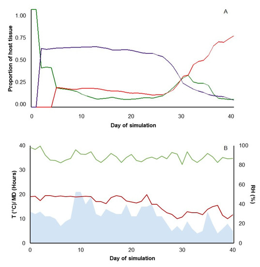
Figure 2.
A representative simulation of the model, which predicts the control of a foliar pathogen following application of a biocontrol agent. (A) Example of one simulation that shows the dynamics for three categories of host tissue: healthy-susceptible tissue (HS, green line); infectious tissue (I, red line); and BCA colonized tissue (Hb, violet line). The simulation refers to the application of a BCA as a preventative treatment for a simulation period of 40 days. (B) Weather conditions used as input in this simulation: temperature (T, °C, red line); moisture duration (MD, h, light-blue area); and relative humidity (RH, %, green line).
An additional state variable, the area under the disease progress curve (AUDPC) [40], was calculated to evaluate the overall effects of BCA characteristics and usage and of environmental conditions on the disease development. The AUDPC was calculated at a daily rate (RAUDPC) as the sum of the total K units of plant tissue occupied by the pathogen (POCC), as follows:
AUDPC = I + R + Ib + Rb.
3. Model Parametrization
The model was parametrized for the biocontrol of BBR in grapevine clusters during ripening, which is between “veraison” (growth stage GS83, [44]) and “berries ripe for harvest” (GS89). The simulation period was set at 40 days, with northern Italy as the reference environment [45]. K units are single berries, which can dynamically belong to one of the seven categories (state variables) of the model. Since the number of berries is already defined at the beginning of the simulation period (K = 1) and does not change because of plant growth from GS83 to GS89, relative rate of growth (RRG) was set to 0 for the entire simulation. Since we assumed that no berries become resistant to B. cinerea infection because of senescence during that growth stage, relative rate of senescence (RRS) was set to 0 for the entire simulation.
During ripening, BBR can develop under favorable weather conditions through three main pathways: (i) latent infections become visible as rotted berries, (ii) air-borne conidia germinate on and infect berries, and (iii) aerial mycelium produced on rotted berries infects adjacent healthy berries (berry-to-berry infection) [46,47]. In the current study, we considered that latent infections and resulting berry-to-berry infections are more common than conidial infections [47,48,49,50,51]. We then assumed that the BBR epidemic starts with the onset of rotted berries that have been latently infected in early growth stages, which constitutes the initial inflow of the pathogen into the system (STARTP). This inflow is assumed to occur on the 4th day of the simulation (i.e., PIN = 4) and to continue for a period of PDUR = 1 day, at a rate RPIN = 0.2 (meaning that 20% of the berries are affected by latent infections).
During the simulation, new berries become affected (i.e., rotted) through the berry-to-berry pathway at the relative rate b, which is calculated by using Equation (17a), following Ciliberti et al. [52]. We assumed that as berries become affected, they begin producing conidia and enter in the I category. Afterwards, the affected berries continue producing conidia until harvest [46]; therefore, there is no outflow from I to R and h = 0.
Two BCAs with different multiple MOA (i.e., having different PROFs) were entered in the system (i.e., BCAs are applied to clusters) in different simulation runs. Specifically, the MOA profile of the first BCA is PROF = P (0.0) + C (0.8) + A (0.2) + IR (0.0). This profile can represent, for example, Aureobasidium pullulans, which is effective against B. cinerea by competing for nutrients at the infection site, which is its main MOA, and also by releasing hydrolytic enzymes that inhibit the pathogen [53,54]. The MOA profile of the second BCA is PROF = P (0.8) + C (0.2) + A (0.0) + IR (0.0). This MOA profile can represent, for example, Pythium oligandrum, which is mainly a mycoparasite but which also competes for nutrients with pathogens [55].
In the model, the overall BCA efficacies (EFF0, EFF1, and EFF2) in preventing the infection are considered at their maximal (i.e., EFF0, EFF1, EFF2 = 1), meaning that tissue colonized by the BCA totally prevents or reduces B. cinerea development.
Both BCAs are applied to clusters as a preventative treatment on the 1st day of simulation (BIN = 1) or as a curative treatment on the 7th day (BIN = 7). These applications constitute the initial inflow of the BCA into the system (STARTB), which has BDUR = 1 day (i.e., the day of BCA application) at a rate RBIN = 0.6 (meaning that the BCA covers 60% of the K units at the time of application).
Parameters of driving functions for calculating b, GRO, and f were derived from the literature and are indicated in Table 2. Rate b is calculated by using Equation (17a), as in Ciliberti et al. [52]. GRO is calculated by using Equation (17b) and by using different parameter values that describe the different responses to temperature and moisture of nine BCA strains (named S1 to S9, see Table 2).
Table 2.
Parameter estimates of the equations fitting the following relationships: the effects of temperature and relative humidity on b (the relative rate of Botrytis cinerea infection), the effects of temperature and moisture duration on GRO (the relative rate of growth of the BCA), and the effects of temperature and relative humidity on f (the relative rate of BCA mortality).
Finally, rate f is calculated using Equation (23), with different settings of parameter values referring to three temperature and humidity conditions under which the BCA survives (Table 2); these settings simulate different BCA manufacturing processes and/or formulations that result in different survival capabilities under stressful vineyard conditions [56,57].
4. Model Running
The model was used to study the effect of the following sources of variation on BBR development: (i) MOA of the BCA (2 levels: mainly competition and mainly mycoparasitism); (ii) BCA application time (2 levels: preventative and curative); (iii) BCA strain (9 levels: 3 ranges of temperatures combined with 3 moisture requirements for BCA growth); and (iv) BCA survival capability (3 levels: low, medium, and high). These sources of variation generate 108 combinations (2 MOAs × 2 application times × 9 strains × 3 survival capabilities). In addition, a situation with no BCA application was considered as the untreated control (NT). To study the effects of environmental conditions, each combination was run under nine scenarios that reflect three climate types with three scenarios per type: (i) warm and dry, (ii) mild and semi-arid, and (iii) cold and wet. Scenarios are represented by fluctuating conditions of temperature, relative humidity, and wetness duration (see Table 3). Therefore, 981 model runs were generated: (1 NT + 108 BCA combinations) × 9 climate scenarios.
Table 3.
Summary of the weather data for the nine climate scenarios.
An example of the effect of the previously mentioned sources of variation on the disease dynamics in the three climate types is provided in Figure 3. Each graph shows the simulated proportion of the host tissue occupied by the pathogen (POCC) over the entire simulation period for each climate type (blue lines, cold and wet; green lines, mild and semi-arid; and yellow lines, warm and dry; Figure 3). Simulations of Figure 3 refer to a competitive BCA (Figure 3A,B) or to a mycoparasitic BCA (Figure 3C,D) applied as a preventative treatment (Figure 3A,C) or as a curative treatment (Figure 3B,D), with the temperature and moisture requirements of S8 and with low survival capability (Table 2). In the cold and wet climate type, BCA application reduced the final (i.e., at day 40) value of POCC by 11% to 16%. In the mild and semi-arid climate type, BCA application reduced the final value of POCC by 53% to 68%, irrespective of application time or MOA. In the warm and dry climate type, BCA application reduced the final value of POCC by 40% to 45%.
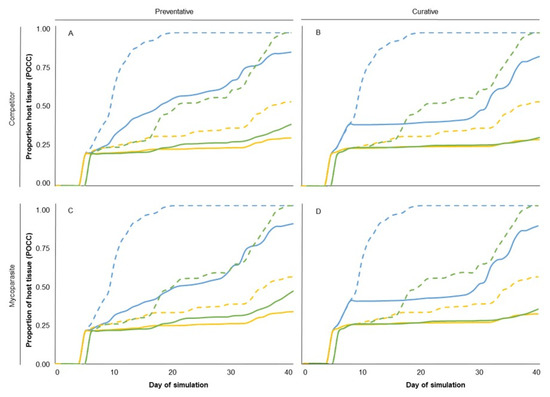
Figure 3.
Examples of the total tissue occupied by the pathogen (POCC) as affected by MOA, application time, and climate type. (A) A mainly competitive BCA applied as a preventative treatment, (B) A mainly competitive BCA applied as a curative treatment, (C) A mainly mycoparasitic BCA applied as a preventative treatment, and (D) a mainly mycoparasitic BCA applied as a curative treatment. Dashed lines indicate POCC dynamics when no BCA application is applied (NT), and solid lines indicate POCC dynamics when a BCA is applied. Blue, green, and yellow lines indicate the simulation in a cold and wet, mild and semi-arid, and warm and dry climate type, respectively. Each line corresponds to the POCC dynamics averaged across the three scenarios used as replicates for each climate type.
The final values of AUDPC simulated for each of the 981 runs of the model were used to calculate the efficacy (E) of each BCA combination (T) in relation to the untreated control (NT), as follows: E = (NT – T)/NT. A factorial analysis of variance (ANOVA) was carried out for each climate type to determine whether the efficacy of each BCA combination was significantly affected by the main sources of variation (MOA, application time, strain, and survival capability) or their interactions. The three scenarios per climate type were used as replicates. The ANOVA was conducted by using the function anova of R software (v 3.6.0; R core team, [58]).
Figure 4 summarizes the efficacy of the BCA in controlling BBR for the different simulation runs. Under the cold and wet climate (Figure 4A), in which BBR developed rapidly and occupied all of the host tissue in < 20 days (Figure 3), BCA efficacy ranged from 0% to 99% and was significantly influenced by all of the main sources of variation (p < 0.001) and by the following interactions: MOA × application time, application time × strain, application × survival capability, and strain × survival capability (Table 4). MOA and application time (preventative or curative) accounted for 2.6% and 1.7% of total variance, respectively, and all of the interactions accounted for <1.7% of the total variance (Table 4). Those factors that are greatly affected by environmental conditions (the BCA strain and its survival capability) together accounted for 91% of the total variance (Table 4). The average efficacy was higher for BCAs with medium or high survival capability (Figure 5A) than for BCAs with low survival capability. The average efficacy in the cold and wet climate was higher for S2 and S8 than for S6 (Figure 6).
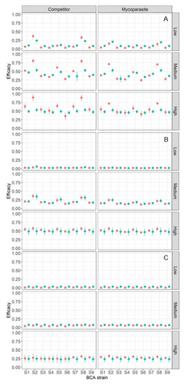
Figure 4.
BCA efficacy against Botrytis bunch rot in ripening grapevine clusters, as affected by MOA (mainly competitor or mainly mycoparasite, as indicated at the top of the figure); responses of 9 BCA strains to temperature (S1 to S9; X axis, see Table 2 for details); BCA survival capability (low, medium, and high, as indicated on the right side of each plot); and climate (A: cold and wet, B: mild and semi-arid, and C: warm and dry). Each point represents the average, and the bars represent the standard errors of three scenarios per each climate type. Red and blue colors indicate that the BCA is applied as a preventative or a curative, respectively, i.e., before or after Botrytis cinerea infection.
Table 4.
Analysis of variance statistics for the influence of MOA, application time, BCA strain, and survival capability on BCA efficacy.
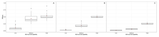
Figure 5.
BCA efficacy against Botrytis bunch rot in ripening grapevine clusters averaged across nine BCA strains and as affected by BCA survival capability (low, medium, and high; see Table 2) and climate type: (A) cold and wet, (B) mild and semi-arid, and (C) warm and dry. The thick line in the boxes is the median, the lowest value in each box represents the 1st quartile (25th percentile), the highest value of each box represents the 3rd quartile (75th percentile), red points in the boxes are the means, and black points in the graph are outliers.
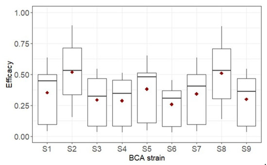
Figure 6.
BCA efficacy against Botrytis bunch rot in ripening grapevine clusters of nine BCA strains (see Table 2) in the cold and wet climate. The thick line in the boxes is the median, the lowest value in each box represents the 1st quartile (25th percentile), the highest value of each box represents the 3rd quartile (75th percentile), red points in the boxes are the means, and black points in the graph are outliers.
Under the mild and semi-arid climate (Figure 4B), in which BBR developed gradually and did not completely occupy the host tissue until the end of the simulation period (Figure 3), BCA efficacy ranged from 1% to 71% and was significantly influenced by the MOA of the BCA (P = 0.017), which accounted for 0.8% of total variance (Table 4), and by the growth requirement of the BCA (as indicated by the strain; p = 0.002), which accounted for 0.4% of total variance (Table 4). BCA efficacy was significantly affected (p < 0.001) by the survival capability of the BCA, which accounted for 97.9% of the total variance (Table 4); BCA efficacy increased with the survival capability of the BCA (Figure 5B).
Under the warm and dry climate (Figure 4C), in which BBR developed slowly and occupied only 50% of the host tissue at the end of the simulation period (Figure 3), BCA efficacy ranged from 0% to 40% and was significantly influenced by the survival capability of the BCA (p < 0.001) and by the interaction between application time and survival capability (P = 0.007), which accounted for 97.3% and 2.2% of total variance, respectively (Table 4). The average efficacy was higher for BCAs with a high survival capability than for BCAs with a low or medium survival capability (Figure 5C). MOA, strain, and application time did not significantly affect BCA efficacy (Table 4).
5. Discussion and Conclusions
The model that was developed by Jeger et al. [28] and that was improved by Xu et al. [29], Xu et al. [30], and Xu and Jeger [31], accounts for the biocontrol mechanisms involved and is able to predict the dynamics of pathogen and biocontrol agent (BCA) populations. In Xu and Jeger [31], the significant effects of varying BCA–temperature relationships and application times on BCA efficacy suggested the importance of considering environmental conditions under which the BCA and target pathogen interact. In the present research, the model of Jeger et al. [28] was enlarged to include crop growth and senescence and the environmental effects on the pathogen and on BCA growth and survival. Like the model of Jeger et al. [28], the enlarged model has a generic structure and can be applied to any pathosystem involving fungal pathogens of aerial plant organs, as well as different pathogen–BCA interactions involving different BCA mechanisms of action.
We parametrized the enlarged model for B. cinerea causing Botrytis bunch rot (BBR) on grapevines. The model parametrization was derived from the epidemiological studies performed by Ciliberti and colleagues [52,59,60]. Those epidemiological relationships were incorporated in a mechanistic model for B. cinerea-grapevine developed by González-Domínguez et al. [47], but the latter model did not include a BCA component. The use of BCAs for BBR control has been extensively studied [61,62,63,64,65,66], with emphasis on biocontrol mechanisms and field efficacy; less research has been conducted to understand how environmental conditions affect BCA fitness and efficacy [11]. In the current study, the model parametrization for BCAs used different parameter values represented by nine BCA strains, which differed in their growth and survival in response to temperature and moisture conditions.
The model was run under three climate types to study the combined effects of the following factors: (i) mechanism of action of the BCA, (ii) timing of BCA application with respect to the pathogen (preventative vs. curative), (iii) temperature and moisture requirements for BCA growth, and (iv) BCA survival capability. All of these factors affected, although to different degrees, biocontrol efficacy. Environmental conditions were the most important factors, accounting for > 90% of the variance in simulated biocontrol efficacy; other factors, even though significant under some climate types, accounted for only a minor percentage of the variance. This finding may help explain why the application of BCAs often results in inconsistent control of the target pathogen in the field [66]. In other words, our results suggest that the inconsistent BCA efficacy in repeated experiments [8,16,67] and in the practical biocontrol of diseases [63,68,69,70] can be caused, at least to some extent, by differences in environmental conditions between experiments or by fluctuations in environmental conditions in the same experiment [1,12,13]. This finding also stresses the importance of considering the environmental response of the BCA during its selection, BCA survival capability during both selection and formulation, and weather conditions and forecasts at the time of BCA application in the field.
Concerning the environmental response of the BCA during its selection, BCAs that are able to grow under a wide range of environmental conditions (i.e., strains S2 and S8 in this study) and that share the temperature and moisture requirements of the target pathogen may be more effective than BCAs with a more limited ability to grow under a range of environmental conditions. BCA responses to temperature and moisture can be evaluated by means of environmentally controlled experiments [71], and the effects of temperature and moisture on the pathogen–BCA relationship can be evaluated by using environmental niches [11]. It is essential that the effects of environments be included when screening BCAs for market development [72,73].
Concerning the BCA survival capability during both selection and formulations, our model simulations indicate that BCAs may be more effective in controlling the target pathogen for long periods and under a range of weather conditions if they have a high rather than a low survival capability. This result confirms previous findings [74,75,76] and also the importance of protective effects provided by additives or adjuvants used in the formulation of the commercial product [56,77,78]. This result also confirms that survival capability should be a key property used to screen microorganisms for biocontrol [73].
Finally, weather conditions and forecasts at the time of BCA application in the field should be considered so as to maximize the probability that the BCA will grow and control the pathogen. Although the current model could be useful in this respect, its utility should be verified with field experiments [79]. On the other hand, developers of BCAs could use the current model to predict the efficacy of candidate organisms under different scenarios of weather conditions and application timings.
Author Contributions
Conceptualization: V.R. and G.F.; methodology: V.R., G.F., and E.G.-D.; formal analysis: G.F. and F.B.; resources: V.R.; writing—original draft preparation: G.F.; writing—review and editing: G.F., F.B., E.G.-D., and V.R.; and supervision: V.R. All authors have read and agree to the published version of the manuscript.
Funding
This research received no external funding.
Acknowledgments
Giorgia Fedele conducted this study within the Doctoral School of the Agro-Food System (Agrisystem) at the Università Cattolica del Sacro Cuore, Piacenza, Italy.
Conflicts of Interest
The authors declare no conflict of interest.
References
- Elad, Y.; Freeman, S. Biological control of fungal plant pathogens. In Agricultural Applications; Kempken, F., Ed.; Springer Berlin Heidelberg: Berlin/Heidelberg, Germany, 2002; pp. 93–109. [Google Scholar]
- Elmer, P.A.G.; Hoyte, S.M.; Vanneste, J.L.; Reglinski, T.; Wood, P.N.; Parry, F.J. Biological control of fruit pathogens. New Zeal. Plant Prot. 2005, 54, 47–54. [Google Scholar] [CrossRef]
- Harman, G.E. Myths and dogmas of biocontrol: Changes in perceptions derived from research on Trichoderma harzianum T-22. Biol. Control 2000, 377–393. [Google Scholar] [CrossRef] [PubMed]
- Tracy, E.F. The promise of biological control for sustainable agriculture: A stakeholder- based analysis. J. Sci. Poly Goverance 2014, 5. [Google Scholar]
- Alavanja, M.C.R.; Hoppin, J.A.; Kamel, F. Health effects of chronic pesticide exposure: Cancer and neurotoxicity. Annu. Rev. Public Health 2004, 25, 155–197. [Google Scholar] [CrossRef] [PubMed]
- Epstein, L. Fifty years since Silent Spring. Annu. Rev. Phytopathol. 2014, 52, 377–402. [Google Scholar] [CrossRef]
- Hahn, M. The rising threat of fungicide resistance in plant pathogenic fungi: Botrytis as a case study. J. Chem. Biol. 2014, 7, 133–141. [Google Scholar] [CrossRef]
- Guetsky, R.; Shtienberg, D.; Elad, Y.; Dinoor, A. Combining biocontrol agents to reduce the variability of biological control. Phytopathology 2001, 91, 621–627. [Google Scholar] [CrossRef]
- Paulitz, T.C.; Belanger, R.R. Biological control in greenhouse systems. Annu. Rev. Phytopathol. 2001, 39, 103–133. [Google Scholar] [CrossRef]
- Rosenheim, J.A.; Kaya, H.K.; Ehler, L.E.; Marois, J.J.; Jaffee, B.A. Intraguild predation among biological-control agents: Theory and evidence. Biol. Control 1995, 5, 303–335. [Google Scholar] [CrossRef]
- Fedele, G.; González-Domínguez, E.; Rossi, V. Influence of environment on the biocontrol of Botrytis cinerea: A systematic literature review. In Strategies to Develop Successful Biocontrol Agents; De Cal, A., Melgarejo, P., Magan, N., Eds.; Springer International Publishing: Cham, Switzerland, 2019; In press. [Google Scholar]
- Kredics, L.; Antal, Z.; Manczinger, L.; Szekeres, A.; Kevei, F.; Nagy, E. Influence of environmental parameters on Trichoderma strains with biocontrol potential. Food Technol. Biotechnol. 2003, 41, 37–42. [Google Scholar]
- Xu, X.; Robinson, J.; Jeger, M.; Jeffries, P. Using combinations of biocontrol agents to control Botrytis cinerea on strawberry leaves under fluctuating temperatures. Biocontrol Sci. Technol. 2010, 20, 359–373. [Google Scholar] [CrossRef]
- Dik, A.J.; Elad, Y. Comparison of antagonists of Botrytis cinerea in greenhouse-grown cucumber and tomato under different climatic conditions. Eur. J. Plant Pathol. 1999, 105, 123–137. [Google Scholar] [CrossRef]
- Elad, Y.; Zimand, G.; Zaqs, Y.; Zuriel, S.; Chet, I. Use of Trichoderma harzianum in combination or alternation with fungicides to control cucumber grey mould (Botrytis cinerea) under commercial greenhouse conditions. Plant Pathol. 1993, 42, 324–332. [Google Scholar] [CrossRef]
- Hannusch, D.; Boland, G.J. Interactions of air temperature, relative humidity and biological control agents on grey mold of bean. Phytopathology 1996, 86, 156. [Google Scholar] [CrossRef]
- Jackson, M.; Whipps, M.; Lynch, M. Effects of temperature, pH and water potential on growth of four fungi with disease biocontrol potential. World J. Microbiol. Biotechnol. 1991, 7, 494–501. [Google Scholar] [CrossRef] [PubMed]
- Mitchell, J.K.; Jeger, J.M.; Taber, R.A. The effect of temperature on colonization of Cercosporidium personatum leafspot of peanuts by the hyperparasite Dicyma pulvinata. Agric. Ecosyst. Environ. 1987, 18, 325–332. [Google Scholar] [CrossRef]
- Deacon, J.W.; Berry, L.A. Biocontrol of soil-borne plant pathogens: Concepts and their application. Pestic. Sci. 1993, 37, 417–426. [Google Scholar] [CrossRef]
- Whipps, J.M. Developments in the Biological Control of Soil-Borne Plant Pathogens. In Advances in Botanical Research; Callow, J.A., Ed.; Academic Press: Cambridge, MA, USA, 1997; Volume 26, pp. 1–134. [Google Scholar]
- Cabrefiga, J.; Montesinos, E. Analysis of aggressiveness of Erwinia amylovora using disease-dose and time relationships. Phytopathology 2005, 95, 1430–1437. [Google Scholar] [CrossRef]
- Johnson, K.B. Dose-response relationships and inundative biological control. Phytopathology 1994, 780–784. [Google Scholar] [CrossRef]
- Montesinos, E.; Bonaterra, A. Dose-response models in biological control of plant pathogens: An empirical verification. Phytopathology 1996, 464–472. [Google Scholar] [CrossRef]
- Smith, K.P.; Handelsman, J.; Goodman, R.M. Modeling dose-response relationships in biological control: Partitioning host responses to the pathogen and biocontrol agent. Phytopathology 1997, 87, 720–729. [Google Scholar] [CrossRef] [PubMed]
- Cunniffe, N.J.; Gilligan, C.A. A theoretical framework for biological control of soil-borne plant pathogens: Identifying effective strategies. J. Theor. Biol. 2011, 278, 32–43. [Google Scholar] [CrossRef] [PubMed]
- Knudsen, G.R.; Hudler, G.W. Use of a computer simulation model to evaluate a plant disease biocontrol agent. Ecol. Modell. 1987, 35, 45–62. [Google Scholar] [CrossRef]
- Kessel, G.J.T.; Köhl, J.; Powell, J.A.; Rabbinge, R.; van der Werf, W. Modeling spatial characteristics in the biological control of fungi at leaf scale: Competitive substrate colonization by Botrytis cinerea and the saprophytic antagonist Ulocladium atrum. Phytopathology 2005, 95, 439–448. [Google Scholar] [CrossRef] [PubMed][Green Version]
- Jeger, M.J.; Jeffries, P.; Elad, Y.; Xu, X.M. A generic theoretical model for biological control of foliar plant diseases. J. Theor. Biol. 2009, 256, 201–214. [Google Scholar] [CrossRef] [PubMed]
- Xu, X.-M.; Salama, N.; Jeffries, P.; Jeger, M.J. Numerical studies of biocontrol efficacies of foliar plant pathogens in relation to the characteristics of a biocontrol agent. Phytopathology 2010, 100, 814–821. [Google Scholar] [CrossRef]
- Xu, X.M.; Jeffries, P.; Pautasso, M.; Jeger, M.J. A numerical study of combined use of two biocontrol agents with different biocontrol mechanisms in controlling foliar pathogens. Phytopathology 2011, 101, 1032–1044. [Google Scholar] [CrossRef]
- Xu, X.-M.; Jeger, M.J. Combined use of two biocontrol agents with different biocontrol mechanisms most likely results in less than expected efficacy in controlling foliar pathogens under fluctuating conditions: A modeling study. Phytopathology 2013, 103, 108–116. [Google Scholar] [CrossRef][Green Version]
- Elad, Y.; Vivier, M.; Fillinger, S. Botrytis, the Good, the Bad and the Ugly. In Botrytis—The Fungus, the Pathogen and its Management in Agricultural Systems; Fillinger, S., Elad, Y., Eds.; Springer International Publishing: Basel, Switzerland, 2016; pp. 1–15. [Google Scholar]
- Jarvis, W.R. Botryotinia and Botrytis Species: Taxonomy, Physiology, and Pathogenicity; Research Branch, Canada Department of Agricolture: Ottawa, ON, Canada, 1977.
- Williamson, B.; Tudzynski, B.; Tudzynski, P.; Van Kan, J.A.L. Botrytis cinerea: The cause of grey mould disease. Mol. Plant Pathol. 2007, 8, 561–580. [Google Scholar] [CrossRef]
- Hethcote, H.W. Three basic epidemiological models. In Applied Mathematical Ecology; Levin, S.A., Hallam, T.G., Grossi, L.J., Eds.; Springer Berlin Heidelberg: Berlin/Heidelberg, Germany, 1989; Volume 18, pp. 119–144. [Google Scholar]
- Leffelaar, P.A.; Ferrari, T.J. Some elements of dynamic simulation. In Simulation and Systems Management in Crop Protection; Van Laar, H.H., Ed.; Pudoc: Wageningen, The Netherlands, 1989; Volume 66, pp. 37–39. [Google Scholar]
- Isee Systems, I. STELLA. System Thinking for Education and Research. Available online: https://www.iseesystems.com/ (accessed on 10 June 2019).
- Forrester, J.W. Industrial Dynamics; M. I. T. Press: Cambridge, UK, 1961. [Google Scholar]
- Rabbinge, R.; de Wit, C.T. Systems, model and simulation. Tetrahedron Lett. 1989, 23, 4461–4464. [Google Scholar]
- Campbell, C.L.; Madden, L.V. Introduction to plant disease epidemiology; John Wiley & Sons.: New York, NY, USA, 1990. [Google Scholar]
- Analytis, S. Über die relation zwischen biologischer entwicklung und temperatur bei phytopathogenen pilzen. J. Phytopathol. 1977, 90, 64–76. [Google Scholar] [CrossRef]
- Reed, K.L.; Hamerly, E.R.; Dinger, B.E.; Jarvis, P.G. An analytical model for field measurement of photosynthesis. J. Appl. Ecol. 1976, 13, 925. [Google Scholar] [CrossRef]
- Wadia, K.D.R.; Butler, D.R. Relationships between temperature and latent periods of rust and leaf-spot diseases of groundnut. Plant Pathol. 1994, 43, 121–129. [Google Scholar] [CrossRef]
- Lorenz, D.H.; Eichhorn, K.W.; Bleiholder, H.; Klose, R.; Meier, U.; Weber, E. Phenological growth stages of the grapevine (Vitis vinifera L. ssp. vinifera)- Codes and descriptions according to the extended BBCH scale. Aust. J. Grape Wine Res. 1995, 1, 100–103. [Google Scholar] [CrossRef]
- Fedele, G.; González-Domínguez, E.; Caffi, T.; Mosetti, D.; Bigot, G.; Rossi, V. Valutazione di un modello matematico per la muffa grigia della vite. In Proceedings of the ATTI Giornate Fitopatologiche, Chianciano Terme, Italy, 6–9 March 2018. [Google Scholar]
- Elmer, P.A.G.; Michailides, T.J. Epidemiology of Botrytis cinerea in orchard and vine crops. In Botrytis: Biology, Pathology and Control; Elad, Y., Williamson, B., Tudzynski, P., Delen, N., Eds.; Springer Netherlands: Dordrecht, The Netherlands, 2007; pp. 243–272. [Google Scholar]
- González-Domínguez, E.; Caffi, T.; Ciliberti, N.; Rossi, V. A mechanistic model of Botrytis cinerea on grapevines that includes weather, vine growth stage, and the main infection pathways. PLoS ONE 2015, 10, 1–23. [Google Scholar] [CrossRef] [PubMed]
- McClellan, W.D. Early Botrytis rot of grapes: Time of infection and latency of Botrytis cinerea Pers. in Vitis vinifera L. Phytopathology 1973, 63, 1151. [Google Scholar] [CrossRef]
- Nair, N.G.; Guilbaud-Oultorfi, S.; Barchia, I.; Emmett, R. Significance of carry over inoculum, flower infection and latency on the incidence of Botrytis cinerea in berries of grapevines at harvest in new south wales. Aust. J. Exp. Agric. 1995, 35, 1177–1180. [Google Scholar] [CrossRef]
- Pezet, R.; Viret, O.; Perret, C.; Tabacchi, R. Latency of Botrytis cinerea Pers.: Fr. and biochemical studies during growth and ripening of two grape berry cultivars, respectively susceptible and resistant to grey mould. J. Phytopathol. 2003, 151, 208–214. [Google Scholar] [CrossRef]
- Keller, M.; Viret, O.; Cole, F.M. Botrytis cinerea infection in grape flowers: Defense reaction, latency, and disease expression. Phytopathology 2003, 93, 316–322. [Google Scholar] [CrossRef]
- Ciliberti, N.; Fermaud, M.; Roudet, J.; Rossi, V. Environmental conditions affect Botrytis cinerea infection of mature grape berries more than the strain or transposon genotype. Phytopathology 2015, 105, 1090–1096. [Google Scholar] [CrossRef]
- Castoria, R.; De Curtis, F.; Lima, G.; Caputo, L.; Pacifico, S.; De Cicco, V. Aureobasidium pullulans (LS-30) an antagonist of postharvest pathogens of fruits: Study on its modes of action. Postharvest Biol. Technol. 2001, 22, 7–17. [Google Scholar] [CrossRef]
- Di Francesco, A.; Ugolini, L.; Lazzeri, L.; Mari, M. Production of volatile organic compounds by Aureobasidium pullulans as a potential mechanism of action against postharvest fruit pathogens. Biol. Control 2015, 81, 8–14. [Google Scholar] [CrossRef]
- Lewis, K.; Whipps, J.M.; Cooke, R.C. Mechanisms of biological disease control with special reference to the case study of Pythium oligandrum as an antagonist. Biotechnol. Fungi Improv. Plant Growth 1989, 16, 191. [Google Scholar]
- Carbó, A.; Torres, R.; Usall, J.; Solsona, C.; Teixidó, N. Fluidised-bed spray-drying formulations of Candida sake CPA-1 by adding biodegradable coatings to enhance their survival under stress conditions. Appl. Microbiol. Biotechnol. 2017, 101, 7865–7876. [Google Scholar] [CrossRef] [PubMed]
- Fu, N.; Chen, X.D. Towards a maximal cell survival in convective thermal drying processes. Food Res. Int. 2011, 44, 1127–1149. [Google Scholar] [CrossRef]
- Team R Core. R: A Language and Environment for Statistical Computing. 2019. Available online: https://www.r-project.org/ (accessed on 10 June 2019).
- Ciliberti, N.; Fermaud, M.; Languasco, L.; Rossi, V. Influence of fungal strain, temperature, and wetness duration on infection of grapevine inflorescences and young berry clusters by Botrytis cinerea. Phytopathology 2015, 105, 325–333. [Google Scholar] [CrossRef]
- Ciliberti, N.; Fermaud, M.; Roudet, J.; Languasco, L.; Rossi, V. Environmental effects on the production of Botrytis cinerea conidia on different media, grape bunch trash, and mature berries. Aust. J. Grape Wine Res. 2016, 22, 262–270. [Google Scholar] [CrossRef]
- Abbey, J.A.; Percival, D.; Abbey, L.; Asiedu, S.K.; Schilder, A. Biofungicides as alternative to synthetic fungicide control of grey mould (Botrytis cinerea)—Prospects and challenges. Biocontrol Sci. Technol. 2019, 29, 207–228. [Google Scholar] [CrossRef]
- Elad, Y.; Stewart, A. Microbial control of Botrytis spp. In Botrytis: Biology, Pathology and Control; Elad, Y., Williamson, B., Tudzynski, P., Delen, N., Eds.; Springer Netherlands: Dordrecht, The Netherlands, 2007; pp. 223–241. [Google Scholar]
- Elmer, P.A.G.; Reglinski, T. Biosuppression of Botrytis cinerea in grapes. Plant Pathol. 2006, 55, 155–177. [Google Scholar] [CrossRef]
- Sharma, R.R.; Singh, D.; Singh, R. Biological control of postharvest diseases of fruits and vegetables by microbial antagonists: A review. Biol. Control 2009, 50, 205–221. [Google Scholar] [CrossRef]
- Jacometti, M.A.; Wratten, S.D.; Walter, M. Review: Alternatives to synthetic fungicides for Botrytis cinerea management in vineyards. Aust. J. Grape Wine Res. 2010, 16, 154–172. [Google Scholar] [CrossRef]
- Haidar, R.; Fermaud, M.; Calvo-Garrido, C.; Roudet, J.; Deschamps, A. Modes of action for biological control of Botrytis cinerea by antagonistic bacteria. Phytopathol. Mediterr. 2016, 33, 13–34. [Google Scholar]
- Shtienberg, D.; Elad, Y. Incorporation of weather forecasting in integrated, biological-chemical management of Botrytis cinerea. Phytopathology 1997, 87, 332–340. [Google Scholar] [CrossRef] [PubMed]
- Fravel, D. Hurdles and bottlenecks on the road to biocontrol of plant pathogens. Australas. Plant Pathol. 1999, 28, 53–56. [Google Scholar] [CrossRef]
- Huang, H.C.; Bremer, E.; Hynes, R.K.; Erickson, R.S. Foliar application of fungal biocontrol agents for the control of white mold of dry bean caused by Sclerotinia sclerotiorum. Biol. Control 2000, 18, 270–276. [Google Scholar] [CrossRef]
- Stewart, A. Commercial biocontrol—Reality or fantasy? Australas. Plant Pathol. 2001, 30, 127–131. [Google Scholar] [CrossRef]
- Fedele, G.; González-Domínguez, E.; Caffi, T.; Rossi, V. Use of environmental niches to understand interactions among Botrytis cinerea, biocontrol agents, and the environment. In Proceedings of the IOBC Bulletin, Vila Real, Portugal, 5–8 November 2019. [Google Scholar]
- Calvo-Garrido, C.; Haidar, R.; Roudet, J.; Gautier, T.; Fermaud, M. Pre-selection in laboratory tests of survival and competition before field screening of antagonistic bacterial strains against Botrytis bunch rot of grapes. Biol. Control 2018, 124, 100–111. [Google Scholar] [CrossRef]
- Köhl, J.; Postma, J.; Nicot, P.; Ruocco, M.; Blum, B. Stepwise screening of microorganisms for commercial use in biological control of plant-pathogenic fungi and bacteria. Biol. Control 2011, 57, 1–12. [Google Scholar] [CrossRef]
- Magan, N. Ecophysiology of biocontrol agents for improved competence in the phyllosphere. Microbial Ecol. Aerial Plant Surfaces 2006. [Google Scholar] [CrossRef]
- Calvo-Garrido, C.; Viñas, I.; Usall, J.; Rodríguez-Romera, M.; Ramos, M.C.; Teixidó, N. Survival of the biological control agent Candida sake CPA-1 on grapes under the influence of abiotic factors. J. Appl. Microbiol. 2014, 117, 800–811. [Google Scholar] [CrossRef]
- Longa, C.M.O.; Pertot, I.; Tosi, S. Ecophysiological requirements and survival of a Trichoderma atroviride isolate with biocontrol potential. J. Basic Microbiol. 2008, 48, 269–277. [Google Scholar] [CrossRef]
- Calvo-Garrido, C.; Teixidó, N.; Roudet, J.; Viñas, I.; Usall, J.; Fermaud, M. Biological control of Botrytis bunch rot in Atlantic climate vineyards with Candida sake CPA-1 and its survival under limiting conditions of temperature and humidity. Biol. Control 2014, 79, 24–35. [Google Scholar] [CrossRef]
- Lahlali, R.; Jijakli, M.H. Enhancement of the biocontrol agent Candida oleophila (strain O) survival and control efficiency under extreme conditions of water activity and relative humidity. Biol. Control 2009, 51, 403–408. [Google Scholar] [CrossRef]
- Gent, D.H.; Mahaffee, W.F.; McRoberts, N.; Pfender, W.F. The use and role of predictive systems in disease management. Annu. Rev. Phytopathol. 2013, 51, 267–289. [Google Scholar] [CrossRef] [PubMed]
© 2020 by the authors. Licensee MDPI, Basel, Switzerland. This article is an open access article distributed under the terms and conditions of the Creative Commons Attribution (CC BY) license (http://creativecommons.org/licenses/by/4.0/).