Determining Irrigation Depths for Soybean Using a Simulation Model of Water Flow and Plant Growth and Weather Forecasts

Abstract

A new scheme to determine irrigation depths using a two-point of predicted cumulative transpiration over irrigation interval is presented. Rather than maximizing water use efficiency, this scheme aims to maximize net income. The volumetric water price is considered to give farmers an incentive to save irrigation water. A field experiment for soybeans was carried out in the Arid Land Research Center, Tottori University, Japan in 2019. The total irrigation amount yield and net income by the proposed scheme were compared to those by a tensiometer-operated automated irrigation. The scheme could save irrigation water by 16% with a yield increment of 20%; resulting in a 22% increase in net income compared to the automated irrigation. The model simulated the volumetric water content in the effective root zone of the plant in fair agreement. These results indicate the effectiveness of the proposed scheme that may replace an automated irrigation system even considering uncertainty in weather forecast to determine irrigation depth and secure investment costs.

1. Introduction

Irrigation is a vital practice for enhancing the global agricultural production under population growth and climatic change. Not only for arid and semi-arid regions, it is sometimes used in humid and sub-humid regions to replenish the reduction of soil water during drought spells in order to maintain yield [1]. Recently, water scarcity is getting serious as it threatens the future of world food production as more than 40% of the world’s population lives in areas experiencing high water stress [2]. Therefore, irrigation under such conditions will have to be managed most efficiently to achieve maximum productivity from limited water.

In order to improve water productivity (WP), both irrigation amount and irrigation timing must be carefully determined considering weather, crop, and soil characteristics. This process is called irrigation scheduling (IS). The development of soil water monitoring technologies has provided better irrigation management. Using such technologies, automated irrigation systems have been developed. Several studies emphasize the effectiveness of such systems on water productivity [3,4,5]. However, these systems require high investments and cannot consider rain until next irrigation. Another attempt to improve WP is deficit irrigation (DI) which may be defined as the application of irrigation below crop water requirements [6]. Numerous studies have shown the benefits of DI on improving WP [7,8]. However, DI is not necessarily beneficial as it is quite difficult to know in prior the optimum percentage of ET deficit which differs from one combination of soil, crop, and climate to another. In addition, DI may be valid only under situations of very severe water scarcity or very expensive water prices as WP is generally defined as yield or income divided by the total amount of irrigation. Some researchers reported that they obtained no significant reduction in yield under deficit irrigation. Those works should be regarded as reevaluation of crop water requirement rather than deficit irrigation studies.

Computer simulation models may be used for optimization of IS. Roy et al. [9] used the HYDRUS-2D model for water flow simulation and DSSAT model for crop simulation with a multi-objective optimization to improve water use efficiency and maximize corn production. Fu et al. [10] used the Soil and Water Assessment Tool (SWAT) software to simulate 16 IS for corn and soybeans in each growth stage based on a combination of effective rainfall, crop water needs, and the sensitive index of crop water production function. In a comparison study between full and deficit irrigation, Adeboye et al. [11] used the AquaCrop model to predict yield, WP, evapotranspiration, soil water content, canopy cover, and crop biomass. One of the benefits of the use of numerical model is that they allow prediction of water flow and crop response in coming days in addition to estimating current status. To predict water flow, we need weather conditions in those days.

Quantitative weather forecast is now freely accessible online and can be used as an input for simulation models to predict future crop water requirements. Lorite et al. [12] used both short-term and long-term weather forecast to determine reference evapotranspiration for maize crop in Spain. Similar averaged values of IS and yield simulation based on forecasted and measured data could manifest the effectiveness of weather forecast for better IS. Still, forecasting evapotranspiration only is not enough to optimize irrigation depth. In other words, optimization of irrigation should meet the motivation of farmers’ work. They apply water to maximize net income, not necessarily yield nor WP, which is the subtraction of total cost from total income. In other words, there would be no motivation for a farmer to save water unless water is priced for each cubic meter.

da Conceição et al. [13] attempted to determine an economically optimum irrigation depth using a polynomial production function based on regression analysis between yield and irrigation depth. They targeted to obtain irrigation depth at gross income rather than net income. They even did not consider weather forecast, but instead used the simple indirect method of [14]. Considering weather forecasts, the genetic algorithm was utilized to solve the couple simulation optimization: Deterministic and stochastic, to determine optimal irrigation depth and maximize seasonal net income [15,16].

In a unique study, an economical irrigation depth corresponding to maximum net income at each irrigation interval, not the entire cropping season, was determined based on a nonlinear relationship between cumulative transpiration and irrigation depth considering weather forecast [17,18]. Their method is somewhat time consuming because it requires three runs of heavy two-dimensional simulation of water flow in a soil. In this study, we present a faster scheme to determine economically optimum irrigation depth assuming a trapezoidal relationship between irrigation depth and cumulative transpiration. Therefore, the objectives of this study were: (1) To determine economical irrigation depths using two predicted points of cumulative transpiration; (2) to check the effectiveness of the proposed scheme compared to an automated irrigation system.

2. Materials and Methods

2.1. Determination of an Economical Irrigation Depth

The optimal irrigation depth is determined through two major steps. First, net income, $I_{\mathrm{n}}$ ($ ha⁻¹), is calculated on the assumption that cumulative transpiration at each irrigation interval can be estimated as:

$$I_{\mathrm{n}}=P_{\mathrm{c}}{\mathsf{\epsilon }\mathsf{\tau }}_{\mathrm{i}}{k}_{\mathrm{i}}-P_{\mathrm{w}}W-C_{\mathrm{ot}},$$

(1)

where $P_{\mathrm{c}}$ is the producer’s price of crop ($ kg⁻¹ DM), ε is transpiration productivity of the crop (produced dry matter (kg ha⁻¹⁾ divided by cumulative transpiration (kg ha⁻¹)), ${\mathsf{\tau }}_{\mathrm{i}}$ is cumulative transpiration between two irrigation events (1 mm = 10,000 kg ha⁻¹), $k_{\mathrm{i}}$ is the income correction factor, used to avoid underestimation of $I_{\mathrm{n}}$ due to smaller ${\mathsf{\tau }}_{\mathrm{i}}$ values in the initial growth stage compared to later growth stages; $P_{\mathrm{w}}$ is the price of water ($ kg⁻¹), W is the irrigation depth (1 mm = 10,000 kg ha⁻¹), and $C_{\mathrm{ot}}$ is other costs (e.g., fertilizers, labors, etc.) ($ ha⁻¹). The first term represents the gross income and second and third terms are costs.

Second, ${\mathsf{\tau }}_{\mathrm{i}}$ is linearly described as a function of $W$:

$${\mathsf{\tau }}_{\mathrm{i}}={\displaystyle \int }{T}_{\mathrm{r}}\mathrm{dt}=a_{\mathrm{t}}W+{\mathsf{\tau }}_0, W<\frac{{\mathsf{\tau }}_{\max }-{\mathsf{\tau }}_0}{a_{\mathrm{t}}}$$

(2a)

$${\mathsf{\tau }}_{\mathrm{i}}={\mathsf{\tau }}_{\max }, W\ge \frac{{\mathsf{\tau }}_{\max }-{\mathsf{\tau }}_0}{a_{\mathrm{t}}}$$

(2b)

where $T_{\mathrm{r}}$ is the transpiration rate (cm s⁻¹), $a_{\mathrm{t}}$ is a fitting parameter, and ${\mathsf{\tau }}_0$ is τ when W equals zero. Hence, optimal irrigation depth corresponding to maximum $I_{\mathrm{n}}$ is obtained when the first derivative of Equation (1) with regard to W becomes zero. Unlike the nonlinear function as presented by Fujimaki et al. [17] and Abd El Baki et al. [18], it is constant either positive or negative as:

$$\frac{\mathrm{d}{I}_{\mathrm{n}}}{\mathrm{d}W}=a_{\mathrm{t}}{P}_{\mathrm{c}}\mathsf{\epsilon }{k}_{\mathrm{i}}-P_{\mathrm{w}}, W<\frac{{\mathsf{\tau }}_{\max }-{\mathsf{\tau }}_0}{a_{\mathrm{t}}}$$

(3a)

$$\frac{\mathrm{d}{I}_{\mathrm{n}}}{\mathrm{d}W}=-P_{\mathrm{w}}, W\ge \frac{{\mathsf{\tau }}_{\max }-{\mathsf{\tau }}_0}{a_{\mathrm{t}}}$$

(3b)

Therefore, when the right-hand side of Equation (3a) is negative, maximum net income is attained when water is not applied:

$$W=0 \mathrm{when} a_{\mathrm{t}}{P}_{\mathrm{c}}\mathsf{\epsilon }{k}_{\mathrm{i}}-P_{\mathrm{w}}<0$$

(4)

Otherwise, maximum net income is attained at the intersection point between the linear function Equation (2a) and ${\mathsf{\tau }}_0$ is constant Equation (2b), because beyond that point, the slope is always negative.

$$W=\frac{{\mathsf{\tau }}_{\max }-{\mathsf{\tau }}_0}{a_{\mathrm{t}}} \mathrm{when} a_{\mathrm{t}}{P}_{\mathrm{c}}\mathsf{\epsilon }{k}_{\mathrm{i}}-P_{\mathrm{w}}\ge 0$$

(5)

This scheme assumes cumulative transpiration linearly increases with irrigation depth and when it reaches the maximal value which is given by potential transpiration, it becomes constant. Therefore, optimal irrigation depth is determined at the point below in which both transpiration and yield decrease. Parameters ${\mathsf{\tau }}_0$ and $a_{\mathrm{t}}$ are determined from two trials at W = 0 and another W. The second W is set at the half of ${\mathsf{\tau }}_0$ plus cumulative reference ET until next irrigation. The scheme presented by Fujimaki et al. [17] and Abd El Baki et al. [18] assumed a nonlinear relationship between cumulative transpiration and irrigation depth; thereby optimal irrigation depth is determined at a point which gives somewhat lower transpiration and yield than potential values. While the original scheme requires three runs to determine parameter values of τ(W) function, the new scheme requires only two which saves time for running simulation by one-third.

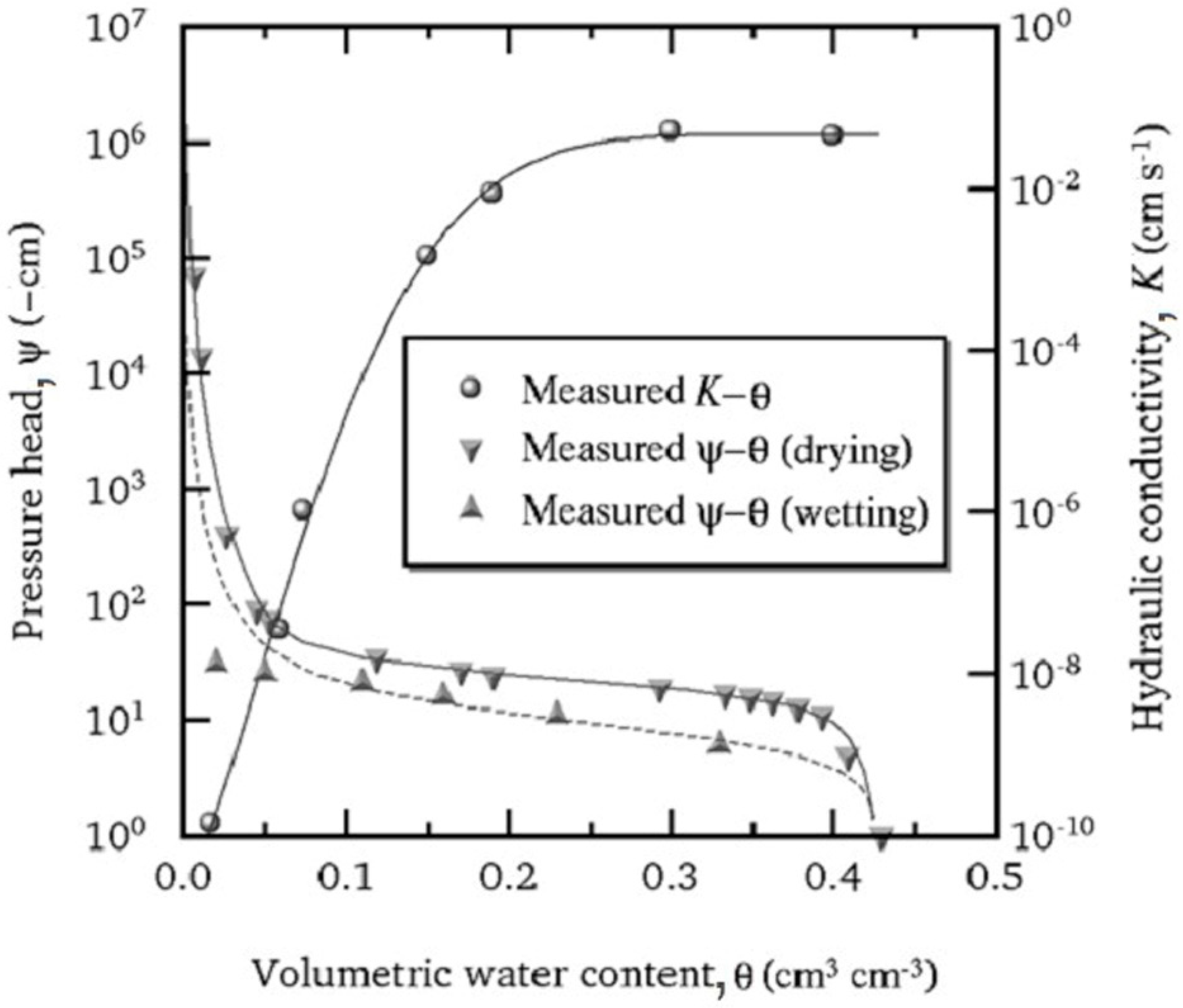
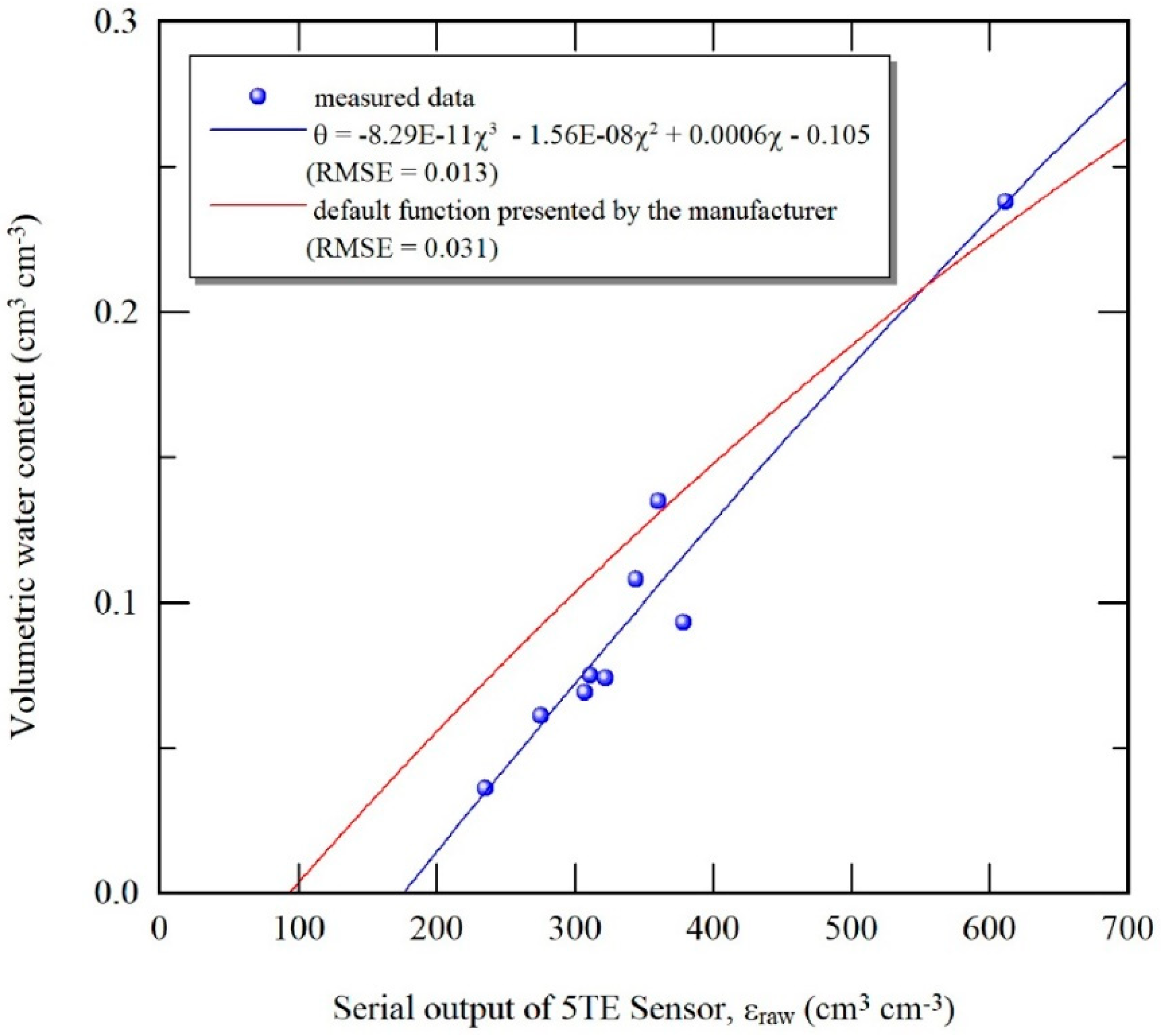
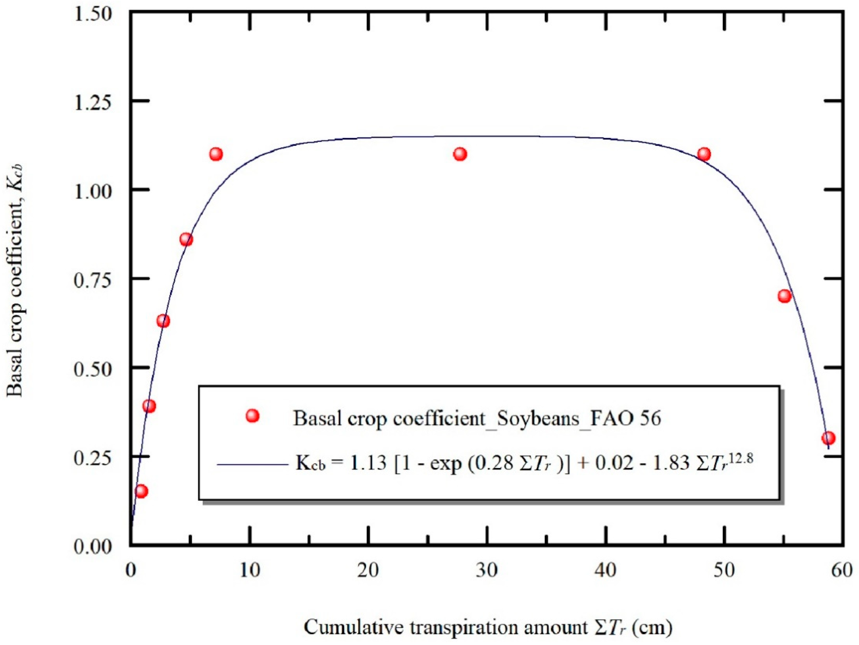
2.2. The Numerical Model

The proposed scheme has been embedded into a numerical model, WASH_2D, which solves equations governing the two-dimensional movement of water, solutes, and heat in soils by the finite difference method. This model can partition evapotranspiration into evaporation and transpiration. Transpiration rate, $T_{\mathrm{r}}$ (cm s⁻¹), was calculated by integrating the water uptake rate, S (cm s⁻¹), over the calculated plant root zone:

$$T_{\mathrm{r}}={L_{\mathrm{x}}}^{-1} {{\displaystyle \int }}_0^{L_{\mathrm{x}}}{{\displaystyle \int }}_0^{L_{\mathrm{z}}}S \mathrm{dxdz}$$

(6)

where $L_{\mathrm{x}}$ and $L_{\mathrm{z}}$ are width and depth of the calculated plant root zone. The values of S were given by the macroscopic root water uptake model [19] as:

$$S=T_{\mathrm{p}}{\mathsf{\beta }\mathsf{\alpha }}_{\mathrm{w}},$$

(7)

where $T_{\mathrm{p}}$, $\mathsf{\beta },$ and ${\mathsf{\alpha }}_{\mathrm{w}}$ are potential transpiration (cm s⁻¹), reduction coefficient, and normalized root density distribution, respectively. The $T_{\mathrm{p}}$ was calculated as follows:

$$T_{\mathrm{p}}=E_{\mathrm{p}}{k}_{\mathrm{cb}},$$

(8)

where $E_{\mathrm{p}}$ is reference evapotranspiration (cm s⁻¹), calculated by the Penman-Monteith Equation [20] and $k_{\mathrm{cb}}$ is basal crop coefficient, which was expressed as a function of cumulative transpiration as:

$$k_{\mathrm{cb}}=a_{\mathrm{kc}}\left[1-\exp \left(b_{\mathrm{kc}}\mathsf{\tau }\right)\right]+c_{\mathrm{kc}}-d_{\mathrm{kc}}{\mathsf{\tau }}^{e_{\mathrm{kc}}},$$

(9)

where $a_{\mathrm{kc}}$, $b_{\mathrm{kc}}$, $c_{\mathrm{kc}}$, $d_{\mathrm{kc}},$ and $e_{\mathrm{kc}}$ are fitting parameters. The $\mathsf{\beta }$ was described as:

$$\mathsf{\beta }=0.75\left(b_{\mathrm{rt}}+1\right)d_{\mathrm{rt}}{}^{-b_{\mathrm{rt}}-1}{\left(d_{\mathrm{rt}}-z+z_{\mathrm{r}0}\right)}^{b_{\mathrm{rt}}}{g}_{\mathrm{rt}}\left(1-x^2{g}_{\mathrm{rt}}{}^{-2}\right),$$

(10)

where $b_{\mathrm{rt}}$ is a fitting parameter; $d_{\mathrm{rt}}$ and $g_{\mathrm{rt}}$ are the depth and width of the plant root zone (cm), respectively; $z$ and $z_{\mathrm{r}0}$ are the soil depth and the depth below which roots exist (cm), respectively; and x is the horizontal distance from the plant (cm). The $d_{\mathrm{rt}}$ is also expressed as a function of $\mathsf{\tau }$ as:

$$d_{\mathrm{rt}}=a_{\mathrm{drt}}\left[1-\exp \left(b_{\mathrm{drt}}\mathsf{\tau }\right)\right]+c_{\mathrm{drt}},$$

(11)

where $a_{\mathrm{drt}}$, $b_{\mathrm{drt}},$ and $c_{\mathrm{drt}}$ are fitting parameters. Using $k_{\mathrm{cb}}$ and $d_{\mathrm{rt}}$ parameters as functions of $\mathsf{\tau }$ instead of days after sowing, the plant growth may be more dynamically responded to drought or salinity stresses through the model. The additive form of the ${\mathsf{\alpha }}_{\mathrm{w}}$ used by the WASH-2D model is a function of drought potential, $\mathsf{\psi }$ (cm) and osmotic potential, ${\mathsf{\psi }}_{\mathrm{o}}$ (cm):

$${\mathsf{\alpha }}_{\mathrm{w}}=\frac{1}{1+{\left(\frac{\mathsf{\psi }}{{\mathsf{\psi }}_{50}}+\frac{{\mathsf{\psi }}_{\mathrm{o}}}{{\mathsf{\psi }}_{\mathrm{o}50}}\right)}^{\mathrm{p}}}$$

(12)

where ${\mathsf{\psi }}_{50}$, ${\mathsf{\psi }}_{\mathrm{o}50,}$ and $\mathrm{p}$ are fitting parameters [21]. Further detailed information regarding the model aspects can be found in [17].

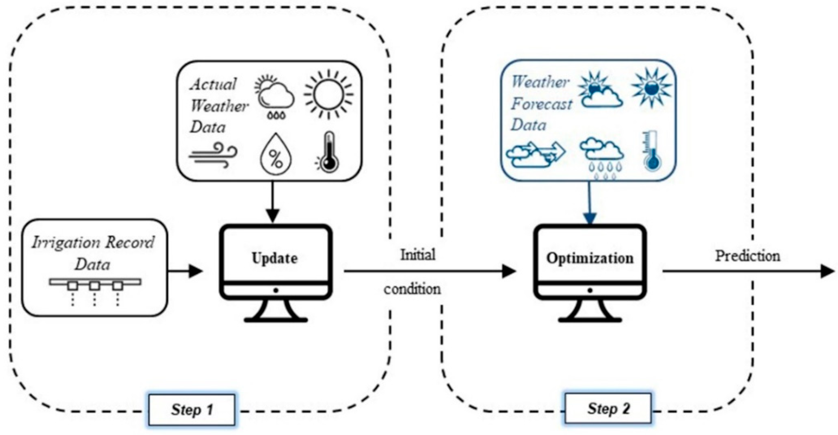
2.3. Implementation of Numerical Simulation for the Proposed Scheme

The determination procedure (Figure 1) starts with updating of the initial condition using a numerical simulation that uses observed weather and irrigation records, and cumulative transpiration at the end of the last run (step 1). Then, by utilizing the results of step 1 in addition to quantitative weather forecast data downloaded from the internet until the next irrigation event, optimal irrigation depth corresponding to maximum net income is determined (step 2). This cycle continues until the final irrigation.

2.4. Field Experiment

A field experiment was carried out at Arid Land Research Center, Tottori, Japan, in 2019. Two treatments were established: (1) Proposed scheme (treatment S), and (2) automated irrigation based on suction monitoring (treatment A). Four replicates were set for each treatment, each replicate was 5 m long and 16 m wide. A drip irrigation system with lateral tubes and emitters spaced at 60 cm and 20 cm, respectively, was installed. In case of the proposed scheme, irrigation interval was set at two-days until August 5 as the available water of sand soil is just 0.05, the plant starts to wilt after two days of irrigation under fine weather, and one-day until the end of irrigation. The automated irrigation system was controlled using three tensiometers at the depth of 20 cm and the trigger value of suction was 40 cm, slightly higher than suction at the field capacity.

Weather data (temperature, wind speed, precipitation, etc.) was collected from a weather station installed in the field while quantitative weather forecast data was downloaded from the website of Yahoo! Japan [22]. The soil was sand with hydraulic properties as shown in Figure 2. To check the accuracy of simulation for volumetric water content, 5TE sensors (METER Inc., USA) were installed at five observation points (x, y): (0, 5), (0, 15), (0, 45) (15, 5), and (30, 5), where x is the horizontal distance from drip tube and z is the soil depth in cm units. Calibration function of the 5TE sensor is shown in Figure 3.

Local Japanese variety of soybean (Glycine max (L.), Fukujishi) was sown on 17 June. The spacing between each plant was 20 cm along the drip tube. The producer price in Japan was set as 3.25 ($ kg⁻¹ FW of shell beans), which was converted into 13.3 ($ kg⁻¹ DM of shell beans). Water price and transpiration productivity were set for numerical simulations at 0.003 and 0.0002 ($ kg⁻¹), respectively. Note that the price of water was similarly set to the one used in Israel [23].

Parameters of crop response function were set according to those reported by Yanagawa and Fujimaki [24] and simply used for numerical simulations. Parameter values of the crop coefficient function were derived from fittings to those reported by Allen et al. [20], when average evapotranspiration during initial, development, mid, and late stages are 3, 4, 5, 5 mm/d, respectively (Figure 4). Other crop parameters were listed in

Table 1. Parameter values of plant growth and stress response function used for the numerical simulation.

Parameter			Remark
$b_{\mathrm{rt}}$	$g_{\mathrm{rt}}$	$z_{\mathrm{r}0}$	Equation (10)
0.12	30	2
$a_{\mathrm{drt}}$	$b_{\mathrm{drt}}$	$c_{\mathrm{drt}}$	Equation (11)
40	−0.4	5
${\mathsf{\psi }}_{50}$	${\mathsf{\psi }}_{\mathrm{o}50,}$	$\mathrm{p}$	Equation (12)
−100	−3000	3

.

Liquid fertilizer (N = 10%, P₂O₅ = 4%, K₂O = 8%) was applied from 25 July until the end of irrigation with a total N rate of 45 kg ha⁻¹. The N is the most determining element for the plant growth, thus the fate of N held by liquid fertilizer was simulated for the entire growing season. Granular fertilizers were also applied occasionally: CaCl₂, (NH₄)₂SO₄, and PK₄₀ (P = 20% and K = 20%) in total rates were 15.4, 45, and 110 kg ha⁻¹, respectively. Both leaf area index (LAI) and above ground biomass (AGB) were measured four times throughout the growing season. Fresh soybean is popular in Japan and our variety is bred for such use; therefore, it was harvested before maturity on 2 September. The yield was statistically analyzed using a randomized complete block design by dividing each plot per treatment into two replicates. The yield as dry seeds were estimated using an oven whose temperature was set at 70 °C. Thereby, each treatment will have four replicates in total. We used MS-Excel 2016 to evaluate significant differences between the two treatments.

3. Results

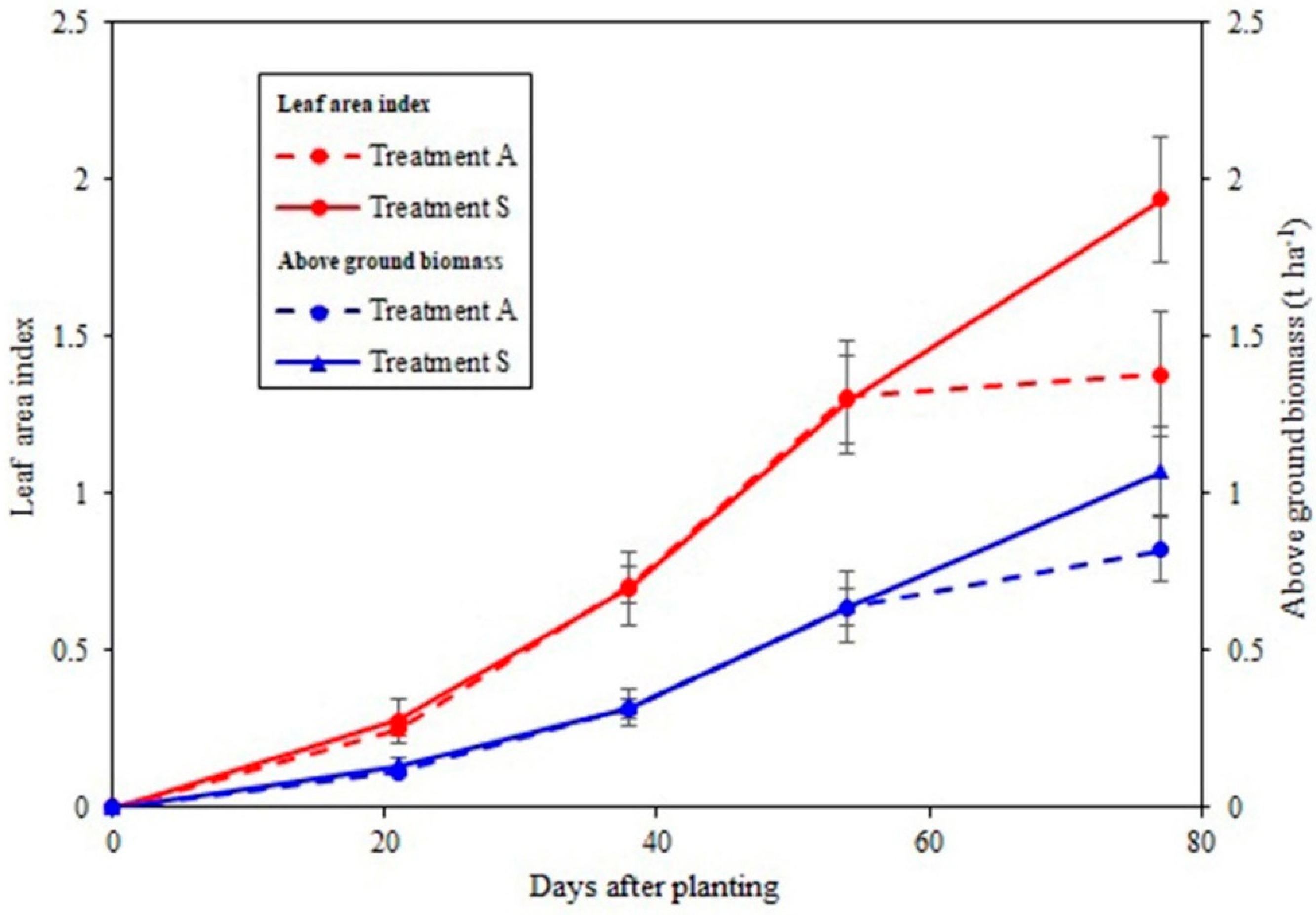
3.1. Leaf Area Index and Biomass

Both LAI and AGB were almost the same until 10 August for both treatments (Figure 5). At the harvest time, treatment S had higher LAI and AGB values than those of treatment A. This might be partly due to higher nutrients uptake for treatment S than treatment A (Figure 6). Especially, nitrogen is the determining element for soybeans growth which is often utilized in the form of NO₃.

According to Figure 6, the uptake of NO₃ was higher for treatment S due to less NO₃ leaching than treatment S. This would be expected as most of the liquid fertilizer was injected at the beginning of irrigation in the automatic irrigation system. The fate of other essential nutrients, potassium, and phosphate ions may also be quite similar. Difficulty in the application of liquid fertilizer at constant concentration may be one of the drawback of automated irrigation systems. LAI values under the two treatments were lower than normal growth in which LAI should be higher than 3.5 by developing a stage to the full pod [25]. This might be due to (1) high losses of nutrients through deep leaching below the plant root zone in sandy soil; and (2) some defoliation was occurred by the insect after 20 August, slightly leading to reduction in leaf dry weight.

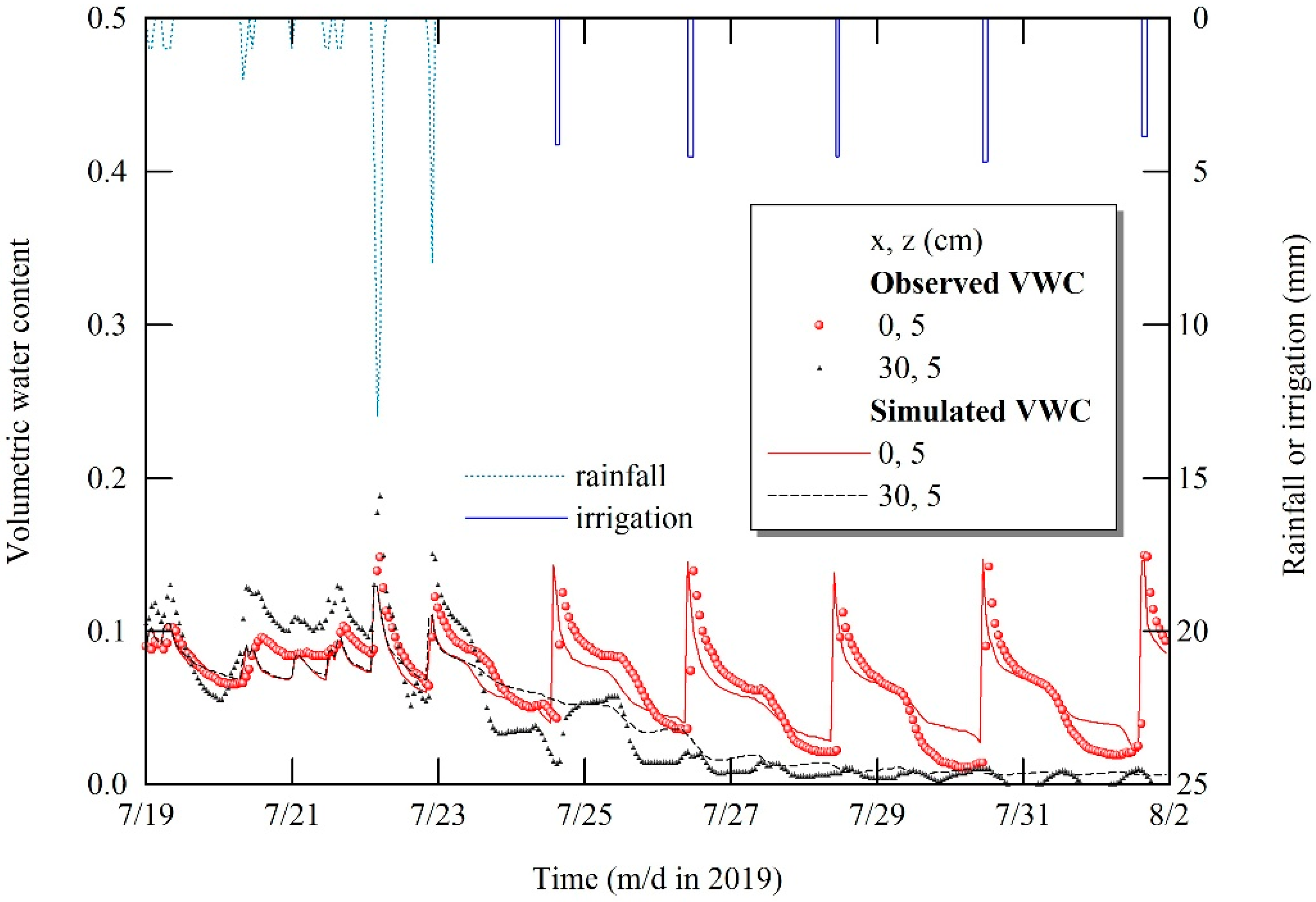
3.2. Soil Water Content

To check the validity of the model in terms of water flow simulation, we compared observed and simulated water contents in two selected points: (0, 5) and (30, 0), as shown in Figure 7. At just below the drip tube (0, 5), the model could estimate VWC after both irrigation and rainfall events with a RMSE of 0.021. In the other observation point (30, 5), where the sensor was in the middle of two adjacent laterals at the depth of 5 cm, the RMSE between observed and simulated VWC values was 0.019. As the soil was sand, water predominantly moves downward rather than horizontally. Therefore, irrigation water cannot reach the surface layer of middle and wet only by rainfall. In general, the model can simulate VWC in fair accuracy in accordance with previous studies [17,18,26,27].

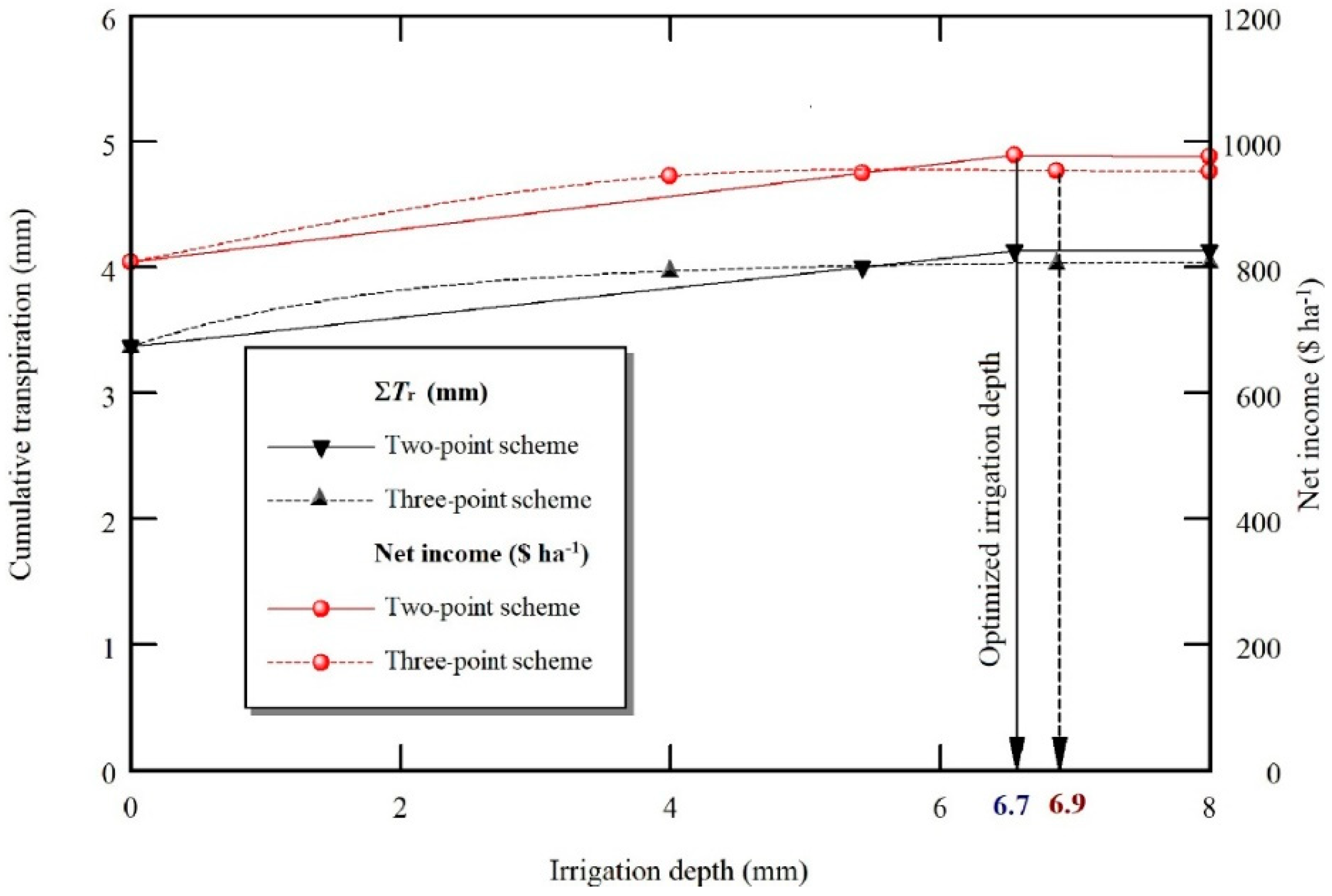
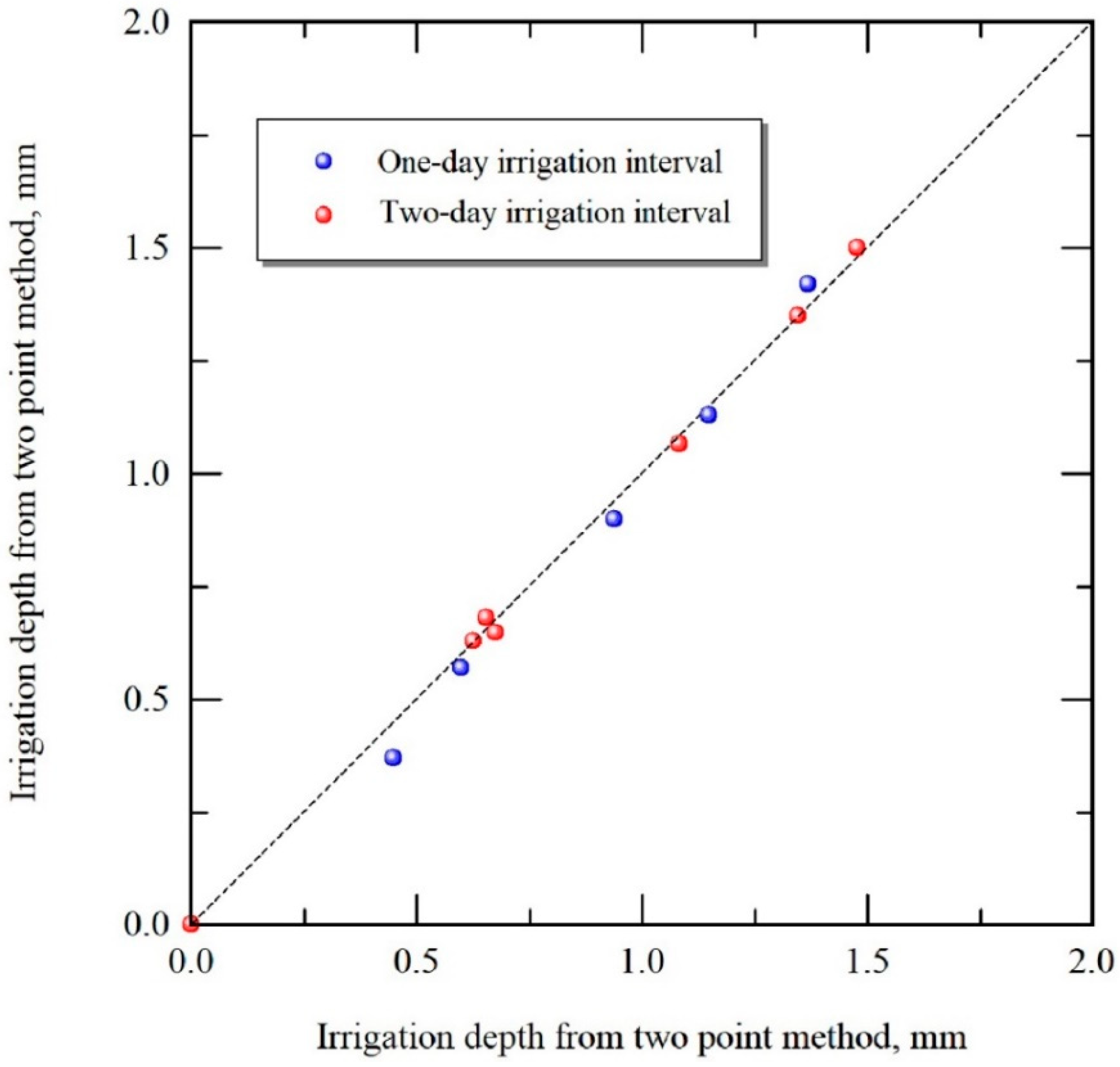
3.3. Example of Determination Optimal Irrigation Depth at Maximal Yield

As shown in Section 2, the proposed scheme uses two predicted points of cumulative transpiration to determine irrigation depth which can be faster than the three-point scheme (Figure 8). On 30 July, the two-point scheme gave 6.7 mm as an optimal irrigation depth which corresponds to both maximum transpiration and maximum net income. On the other hand, the three-point scheme proposed by Fujimaki et al. [17] and Abd El Baki et al. [18] determined the close value of irrigation depth at 6.9 mm which gave maximal net income. The optimal irrigation depths for other irrigation days under either one or two irrigation intervals determined by both schemes were close (Figure 9).

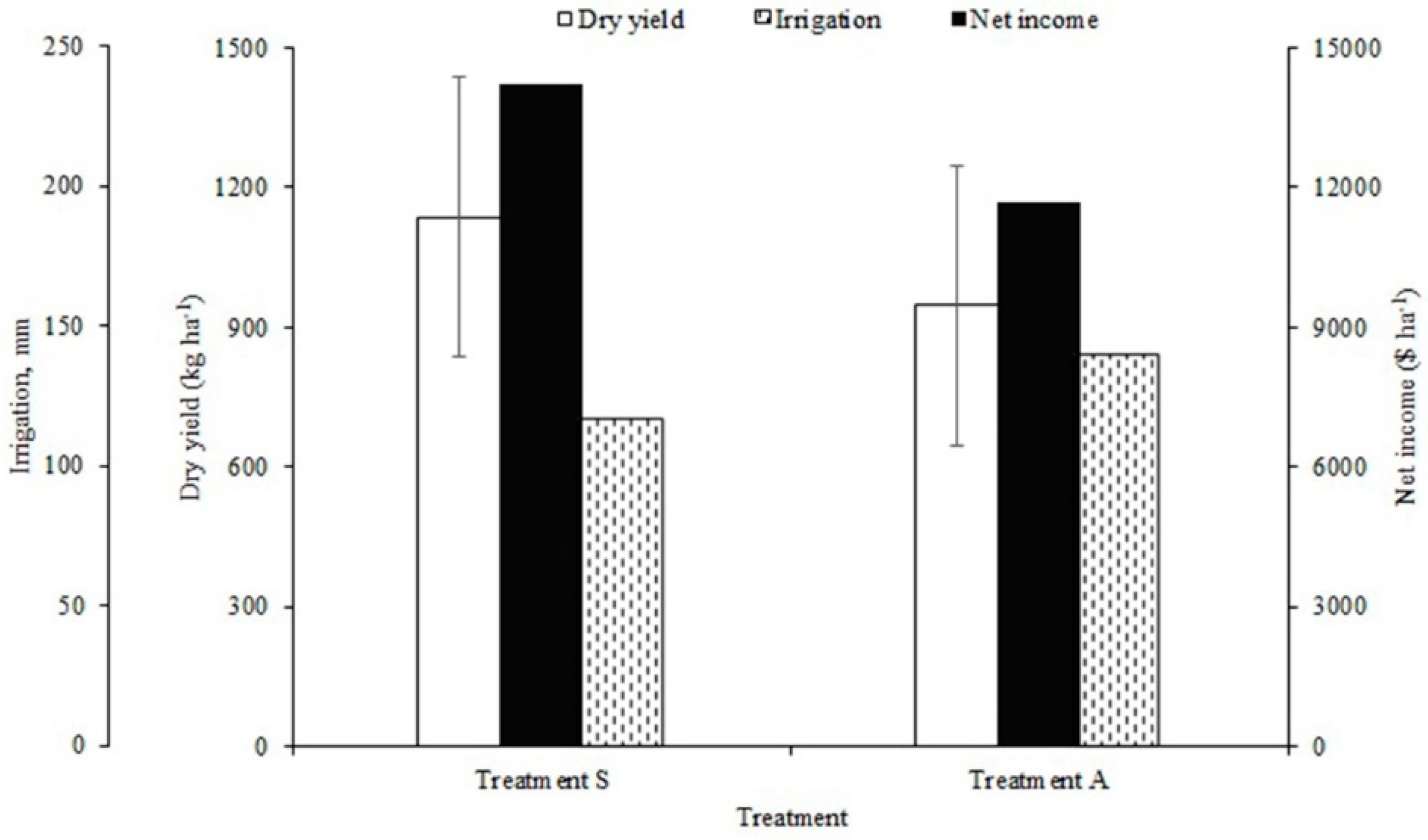
3.4. Net Income and Yield Assessment

The total net income between the two experimental treatments is shown in Figure 10. Total net income increased by 22% for treatment S when the yield was based on the dry pod shell. This was due to both yield increment and water saving by 20% and 16%, compared to treatment A. Some yield parameters were statistically analyzed to check the impact of the proposed scheme on soybean crop production (

Table 2. Statistical analysis for some growth parameters of soybeans.

Treatment	Mass Grain Yield	Crop Height	AGB	LAI
	g	cm	g
Treatment A	47.3 ± 2.2	35.9 ± 0.4	9.2 ± 1.3	1.4 ± 0.2
Treatment S	57.8 ± 2.7 *	37.4 ± 2.3	13.2 ± 1.7	1.9 ± 0.2

Means in each column followed by * indicates significant difference (p ≤ 0.05) and (± SE) indicates to the standard error.

). Fresh pod shell yield of treatment S was significantly higher than treatment A. This may due to greater nutrients uptake which led to a larger transfer of nitrogen from leaves to seeds during the seed filling stage [28]. On the other hand, there were no significant difference for dry seeds, crop height, LAI, and AGB between the two treatments. Although small LAI were attained for both treatments, total fresh pod shell yield was not largely affected in accordance with previous studies in which losses of leaf area values due to the weather or insect did not largely affect soybean yield [29,30].

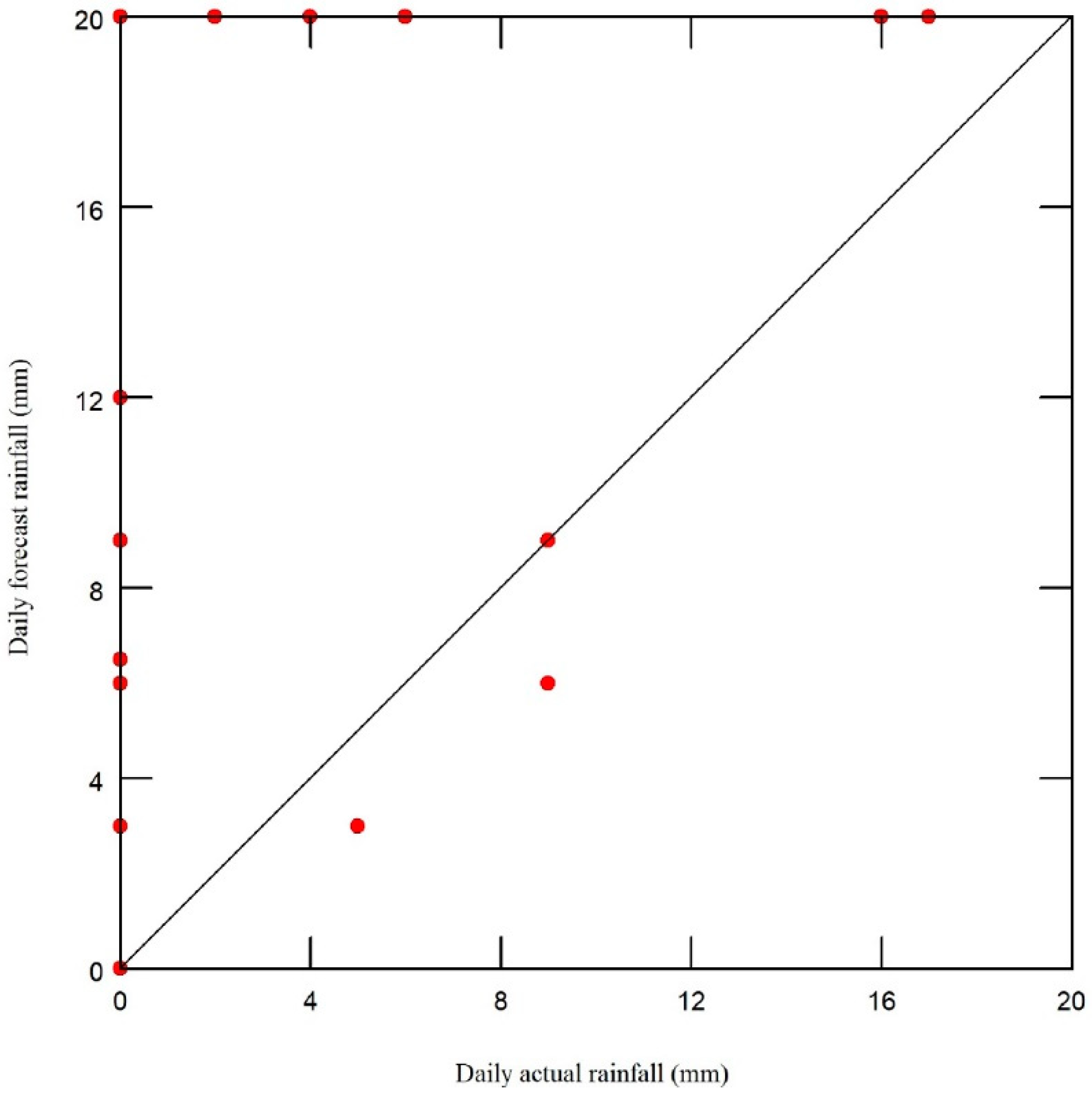
3.5. Accuracy of Weather Forecast

The accuracy of weather forecast plays a great role on the performance of the proposed scheme. The accuracy of most weather factors (e.g., temperature, relative humidity, etc.) are fine, except for rainfall. We compared actual rainfall values with forecasted ones to check the accuracy as shown in Figure 11. We set daily effective rainfall as 20 mm in this comparison. The RMSE was 7.8 mm. The largest error occurred on 28 August when the actual and foretasted rain were 17 and 72 mm, respectively. Note that any value of rainfall greater than 20 mm was set as 20 mm which is effective rain for the soil. As the holding capacity of sandy soil is low, the short-term weather forecast was used. This might have reduced the negative impact of weather forecast. Even under inaccuracy of weather forecast, the proposed scheme may play a positive role to enhance net income.

3.6. Advantages of the Proposed Scheme over Other Methods

Even if net income were not significantly different, as we discussed in the introduction, the determination of irrigation depth to maximize net income during each irrigation interval using WASH_2D can save the cost of soil moisture sensors or tensiometers required for the automated irrigation system. It can consider the forecasts of rainfall and immune from malfunctions. Another potential advantage of the proposed scheme using WASH-2D is that it can also consider salinity stress, as well as drought stress. Further studies are required for evaluating whether the proposed scheme using WASH-2D can also mitigate salinity stress.

Compared with originally presented three-point scheme proposed by Fujimaki et al. [17], the newly proposed two-point scheme can cut computation time by one-third. The two-point scheme took less than one minute (48 s) on the Intel Core i3-8130U CPU for the two-day interval in this study.

4. Conclusions

The proposed scheme using two predicted points of irrigation depth and cumulative transpiration was developed. In this study, the scheme was validated for soybeans grown in a sand field by comparing the automated irrigation system based on suction monitoring. The scheme could save irrigation water by 16%. As water was priced and yield increased by 20%, the total net income increased by 22% compared to the automated irrigation system. The scheme also had a positive impact on nutrients saving, which might have led to higher yield than the automated irrigation system. The model simulated water flow in fair accuracy. The proposed scheme could be a beneficial tool to enhance net income.

References

1. Debaeke, P.; Aboudrare, A. Adaptation of crop management to water-limited environments. Eur. J. Agron. 2004, 21, 433–446. [Google Scholar] [CrossRef]
2. United Nations. SDG 6 Synthesis Report. Water and Salinization for All: Letting Data Lead the Way; United Nations: New York, NY, USA, 2018. [Google Scholar]
3. Boutraa, T.; Akhkha, A.; Alshuaibi, A.; Atta, R. Evaluation of the effectiveness of an automated irrigation system using wheat crops. ABJNA 2011, 2, 80–88. [Google Scholar] [CrossRef]
4. Romero, R.; Muriel, J.L.; Garcia, I.; Green, S.R.; Clothier, B.E. Improving heatpulse methods to extend the measurement range including reverse flows. Acta Hortic. 2012, 951, 31–38. [Google Scholar] [CrossRef]
5. Domínguez-Niño, J.M.; Oliver-Manera, J.; Girona, J.; Casadesús, J. Differential irrigation scheduling by an automated algorithm of water balance tuned by capacitance-type soil moisture sensors. Agric. Water Manag. 2020, 228, 105880. [Google Scholar] [CrossRef]
6. English, M. Deficit irrigation. I. Analytical framework. J. Irrig. Drain. Eng. 1990, 116, 399–412. [Google Scholar] [CrossRef]
7. Zhang, Y.; Hansen, N.; Trout, T.; Nielsen, D.; Paustian, K. Modeling Defcit Irrigation of Maize with the DayCent Model. Agron. J. 2018, 110, 1754–1764. [Google Scholar] [CrossRef]
8. Adeyemi, O.; Grove, I.; Peets, S.; Norton, T. Advanced Monitoring and Management Systems for Improving Sustainability in Precision Irrigation. Sustainability 2017, 9, 353. [Google Scholar] [CrossRef] [Green Version]
9. Roy, P.C.; Guber, A.; Abouali, M.; Nejadhashemi, A.P.; Deb, K.; Smucker, A.J.M. Simulation Optimization of Water Usage and Crop Yield Using Precision Irrigation. In Proceedings of the International Conference on Evolutionary Multi-Criterion Optimization, Michigan, MI, USA, 10–13 March 2019; pp. 695–706, LNCS 11411. [Google Scholar]
10. Fu, Q.; Yang, L.; Li, H.; Li, T.; Liu, D.; Ji, Y.; Li, M.; Zhang, Y. Study on the Optimization of Dry Land Irrigation Schedule in the Downstream Songhua River Basin Based on the SWAT Model. Water J. 2019, 11, 1147. [Google Scholar] [CrossRef] [Green Version]
11. Adeboye, O.B.; Schultz, B.; Adekalu, K.O.; Prasad, K. Modelling of Response of the Growth and Yield of Soybean to Full and Deficit Irrigation by Using AquaCrop. Irrig. Drain. 2017, 66, 192–205. [Google Scholar] [CrossRef]
12. Lorite, I.J.; Ramírez-Cuesta, J.M.; Cruz-Blanco, M.; Santos, C. Using weather forecast data for irrigation scheduling under semi-arid conditions. Irrig. Sci. 2015, 33, 411–427. [Google Scholar] [CrossRef]
13. da Conceição, C.G.; Robaina, A.D.; Peiter, M.X.; Parizi, A.R.C.; da Conceição, J.A.; Bruning, J. Economically optimal water depth and grain yield of common bean subjected to different irrigation depths. Rev. Bras. Eng. Agric. Ambient. 2018, 22, 482–487. [Google Scholar] [CrossRef] [Green Version]
14. Benavides, J.G.; Díaz, J.L. Formula para el calculo de la evapotranspiracion potencial adaptada al tropico (15° N–15° S). Agron. Trop. Mar. 1970, 20, 335–345. [Google Scholar]
15. Wang, D.B.; Cai, X.M. Irrigation scheduling-role of weather forecasting and farmers’ behavior. J. Water Resour. Plan. Manag. 2009, 135, 364–372. [Google Scholar] [CrossRef]
16. Jamal, A.; Linker, R.; Housh, M. Optimal Irrigation with Perfect Weekly Forecasts versus Imperfect Seasonal Forecasts. J. Water Resour. Plan. Manag. 2019, 145, 06019003. [Google Scholar] [CrossRef]
17. Fujimaki, H.; Tokumoto, I.; Saito, T.; Inoue, M.; Shibata, M.; Okazaki, T.; Nagaz, K.; El Mokh, F. Determination of irrigation depths using a numerical model and quantitative weather forecast and comparison with an experiment. In Practical Applications of Agricultural System Models to Optimize the Use of Limited Water; Ahuja, L.R., Ma, L., Lascano, R.J., Eds.; ACSESS: Madison, WI, USA, 2014; Volume 5, pp. 209–235. [Google Scholar]
18. Abd El Baki, H.M.; Fujimaki, H.; Tokumoto, I.; Saito, T. A new scheme to optimize irrigation depth using a numerical model of crop response to irrigation and quantitative weather forecasts. Comput. Electron. Agric. 2018, 150, 387–393. [Google Scholar] [CrossRef]
19. Feddes, R.A.; Raats, P.A.C. Parameterizing the soil-water-plant root system, unsaturated-zone modeling: Progress, challenges, applications. In Wageningen UR Frontis Series; Feddes, R.A., de Rooij, G.H., van Dam, J.C., Eds.; Kluwer Academic: Dordrecht, The Netherlands, 2014; Volume 5. [Google Scholar]
20. Allen, R.; Pereira, L.; Raes, D.; Smith, M. Crop Evapotranspiration: Guidelines for Computing Crop Water Requirements. FAO Irrigation and Drainage Paper No. 56; FAO: Rome, Italy, 1998; pp. 135–142. [Google Scholar]
21. van Genuchten, M.T. A Numerical Model for Water and Solute Movement in and Below the Root Zone, Reserch Report 121, U.S. Salinity Laboratory, Agricultural Research Service; United States Department of Agriculture: Riverside, CA, USA, 1987.
22. Weather and Disaster, Chugoku, Tottori, Eastern Tottori, Iwami-Cho. Available online: https://weather.yahoo.co.jp/weather/jp/31/6910/31302.html (accessed on 2 September 2019).
23. Cornish, G.; Bosworth, B.; Perry, C. Water Charging in Irrigated Agriculture—An Analysis of International Experience; FAO: Rome, Italy, 2004; pp. 19–26. [Google Scholar]
24. Yanagawa, A.; Fujimaki, H. Tolerance of canola to drought and salinity stresses in terms of root water uptake model parameters. J. Hydrol. Hydromech. 2013, 61, 73–80. [Google Scholar] [CrossRef] [Green Version]
25. Westgate, M.E. Managing Soybeans for Photosynthetic Efficiency. In Proceedings of the 4th World Soybean Reserch Conference, Chicago, IL, USA, 4–7 August 1999; Kauffman, H.E., Ed.; pp. 223–228. [Google Scholar]
26. Abd El Baki, H.M.; Fujimaki, H.; Tokumoto, I.; Saito, T. Determination of irrigation depths using a numerical model of crop growth and quantitative weather forecast and evaluation of its effect through a field experiment for potato. J. Jpn. Soc. Soil Phys. 2017, 136, 15–24. [Google Scholar]
27. Abd El Baki, H.M.; Fujimaki, H.; Tokumoto, I.; Saito, T. Optimizing Irrigation Depth Using a Plant Growth Model and Weather Forecast. JAS 2018, 10, 55–66. [Google Scholar] [CrossRef]
28. Sinclair, T.R. Water and Nitrogen Limitations in Soybean Grain Production. Field Crop. Res. 1986, 15, 125–141. [Google Scholar] [CrossRef]
29. Haile, F.; Higley, L.; Specht, J.; Spomer, S. Soybean leaf morphology and defoliation tolerance. Agron. J. 1998, 90, 353–362. [Google Scholar] [CrossRef]
30. Conley, S.P.; Pedersen, P.; Christmas, E.P. Main-stem node removal effect on soybean seed yield and composition. Agron. J. 2009, 101, 120–123. [Google Scholar] [CrossRef]
Figure 1. Implementation procedure of numerical simulations using the WASH-2D model for the proposed scheme (two steps were performed to determine irrigation depths: Update and optimization runs).
Agronomy 10 00369 g001
Figure 2. Soil hydraulic properties for sandy soil, Tottori, Japan.
Agronomy 10 00369 g002
Figure 3. Calibration function for the 5TE sensor in Tottori sandy soil.
Agronomy 10 00369 g003
Figure 4. The relationship between cumulative transpiration and basal crop coefficients throughout the growing season (parameters of the proposed function was acquired by the fitting to Kcb values reported by (Allen et al., 1998)).
Agronomy 10 00369 g004
Figure 5. The cumulative growth of leaf area index (LAI) and above ground biomass (AGB) throughout the growing season (the proposed scheme denotes as treatment S and automated irrigation denotes as treatment A). Error bars represent standard error.
Agronomy 10 00369 g005
Figure 6. The fate of nitrate, NO3, under both treatments throughout the growing season of soybeans (the proposed scheme denotes as treatment S and automated irrigation denotes as treatment A).
Agronomy 10 00369 g006
Figure 7. Comparison between observed and simulated volumetric water content for treatment S (x indicates the horizontal distance apart from the drip tube, z indicates the soil depth).
Agronomy 10 00369 g007
Figure 8. Determination example of irrigation depth in terms of net income on 30 July (cumulative transpiration (mm) and net income ($ ha−1) corresponding to irrigation depth (mm) for the previous and current proposed schemes).
Agronomy 10 00369 g008
Figure 9. Comparison for optimal irrigation depths determined by both schemes for several irrigation days (the simulations were performed based on one-day and two-day irrigation interval).
Agronomy 10 00369 g009
Figure 10. Comparison of total net income, total irrigation amount, and yield between the two treatments (the proposed scheme denotes as treatment S and automated irrigation denotes as treatment A. Error bars represent standard error.
Agronomy 10 00369 g010
Figure 11. Comparison between both actual and forecasted rainfall throughout the growing season.
Agronomy 10 00369 g011