

Selecting EOR Polymers through Combined Approaches—A Case for Flooding in a Heterogenous Reservoir


Abstract
:1. Introduction
2. Approach and General Workflow
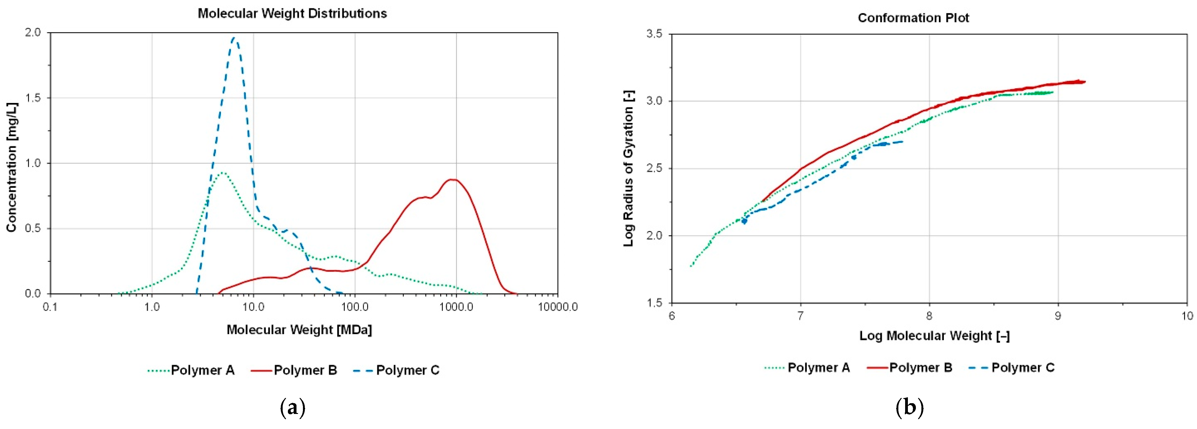
- Quality Assurance/Quality Check of polymer powder by characterization using Field-Flow Fractionation (FFF) analysis, to measure MW as well as full MWD.
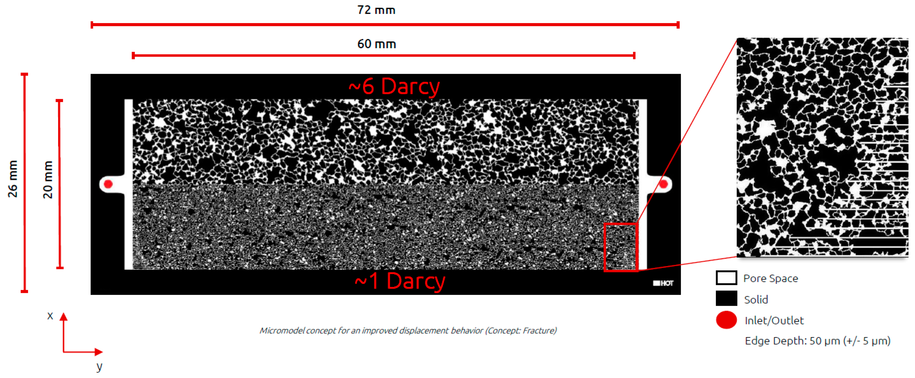
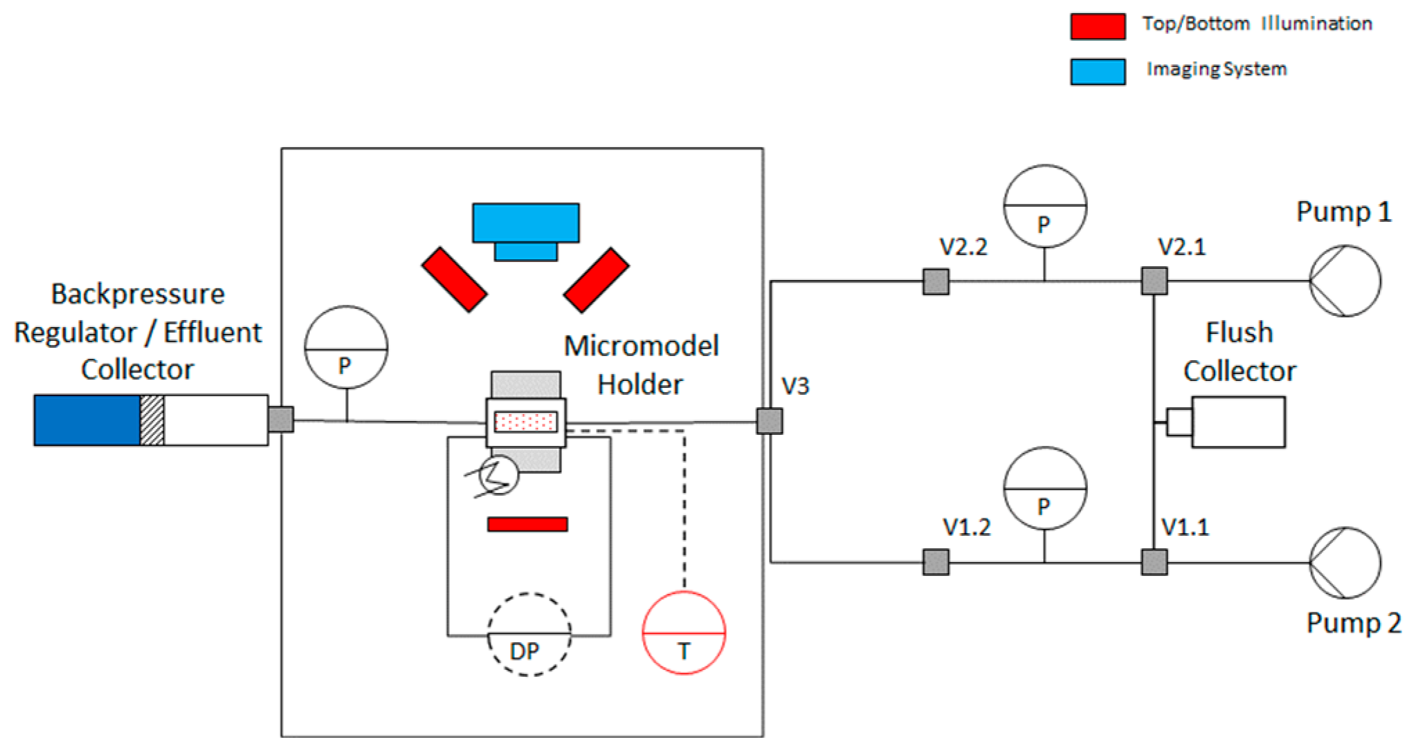
- Two-phase heterogenous micromodel (specially designed) flooding to understand polymer performance in heterogenous environment with reservoir representative injection velocities and reservoir temperature (performed in parallel with single-phase evaluations). This, to gather some early insights in polymer performance in two phase environment before performing time consuming core floods.
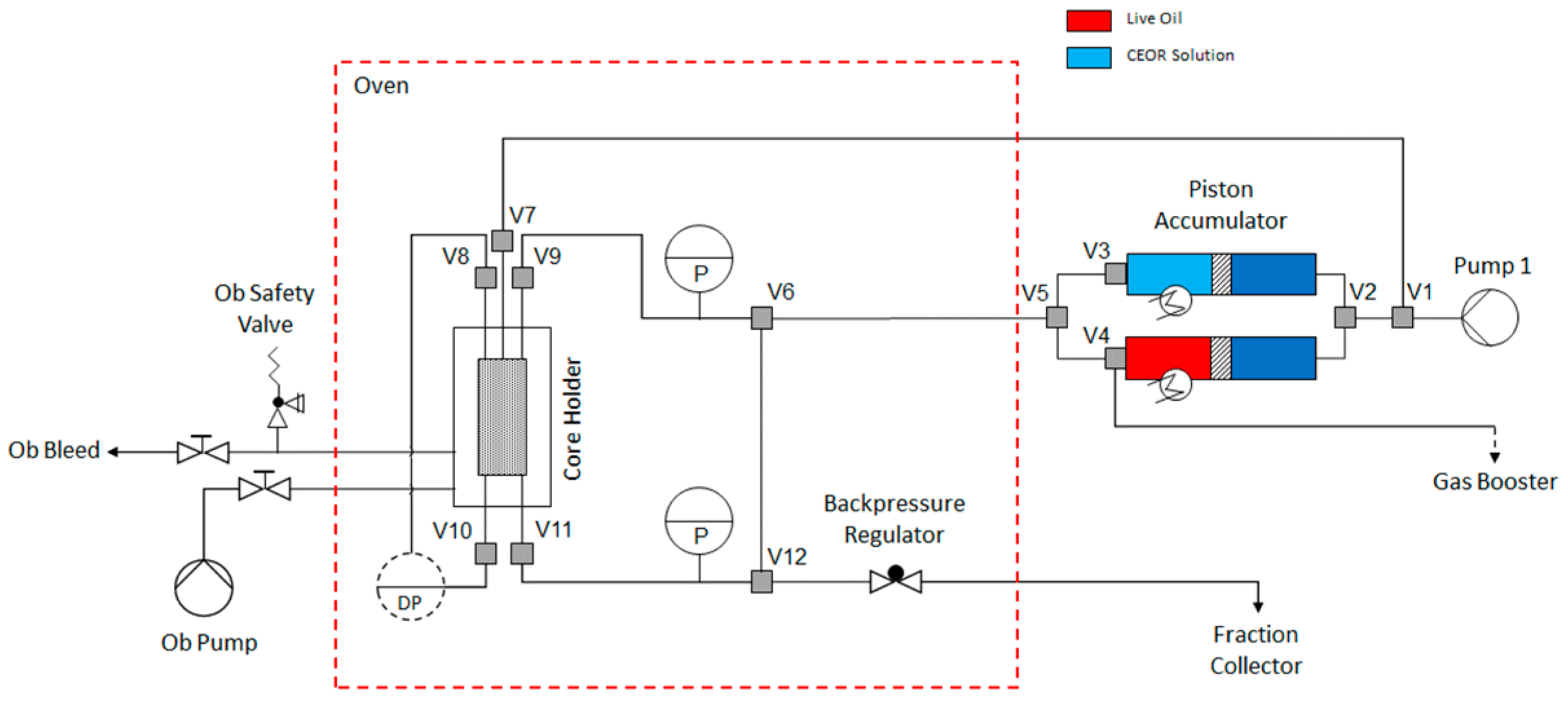
- Single-phase core flood experiments were performed to understand the behavior of selected polymers at near-wellbore conditions. Outcrop samples matching lower range field permeability were used. Effluent samples were analyzed by FFF which gave insights into polymer flow in porous medium.
- Two phase core flooding to capture polymer performance deep within the reservoir and displacement efficiency.
- Polymer selection and recommendation for field usage/application.
3. Materials and Methods
- 6.
- Saturate the micromodel 100% with synthetic formation brine,
- 7.
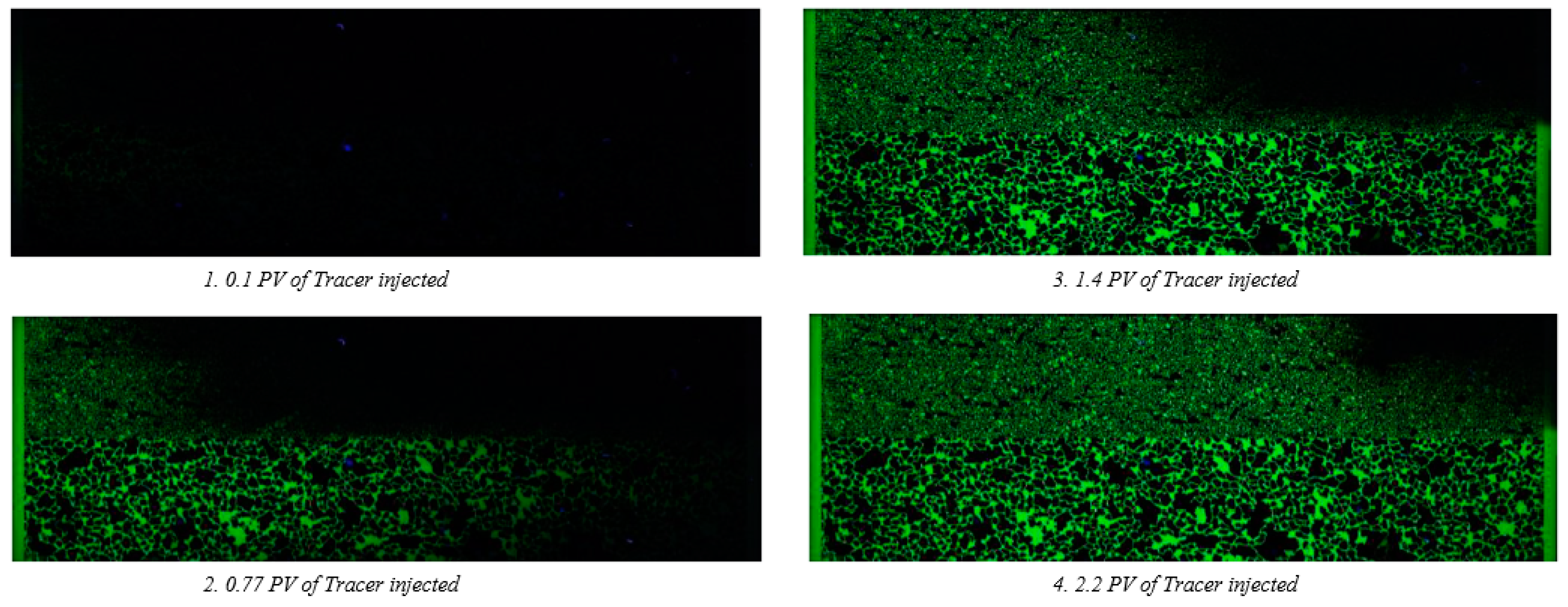
- Inject visual tracer to see the front propagation in different layers (performed once),
- 8.
- Displace visual tracer with synthetic formation brine,
- 9.
- Displace the brine with viscosity matched oil,
- 10.
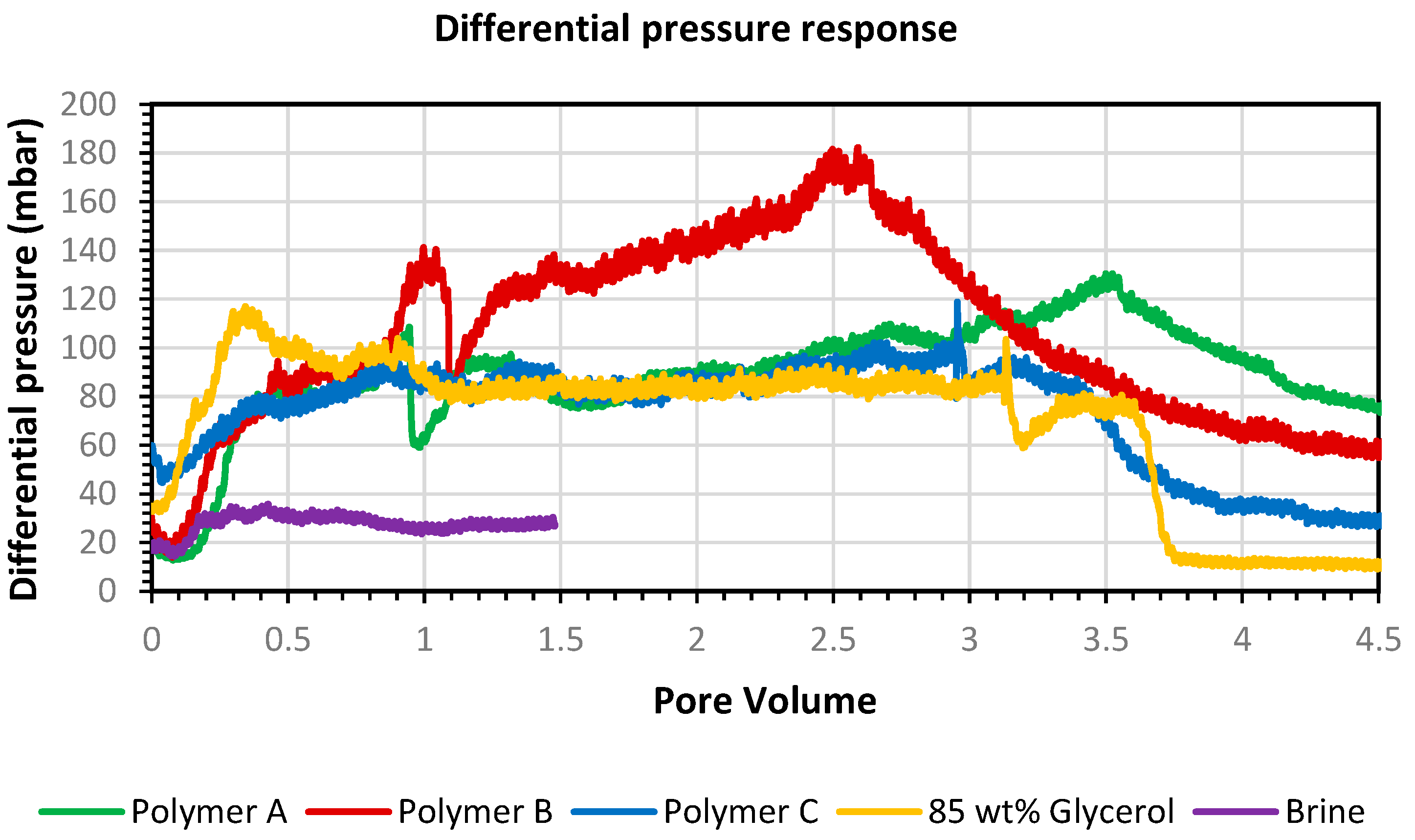
- Depending on experiment, inject desired solution for ~3.5 pore volume (PV) (synthetic formation brine or Polymer solutions or viscosity matched Glycerol solution),
- 11.
- Follow up with synthetic formation brine for ~1.5 PV.
- 12.
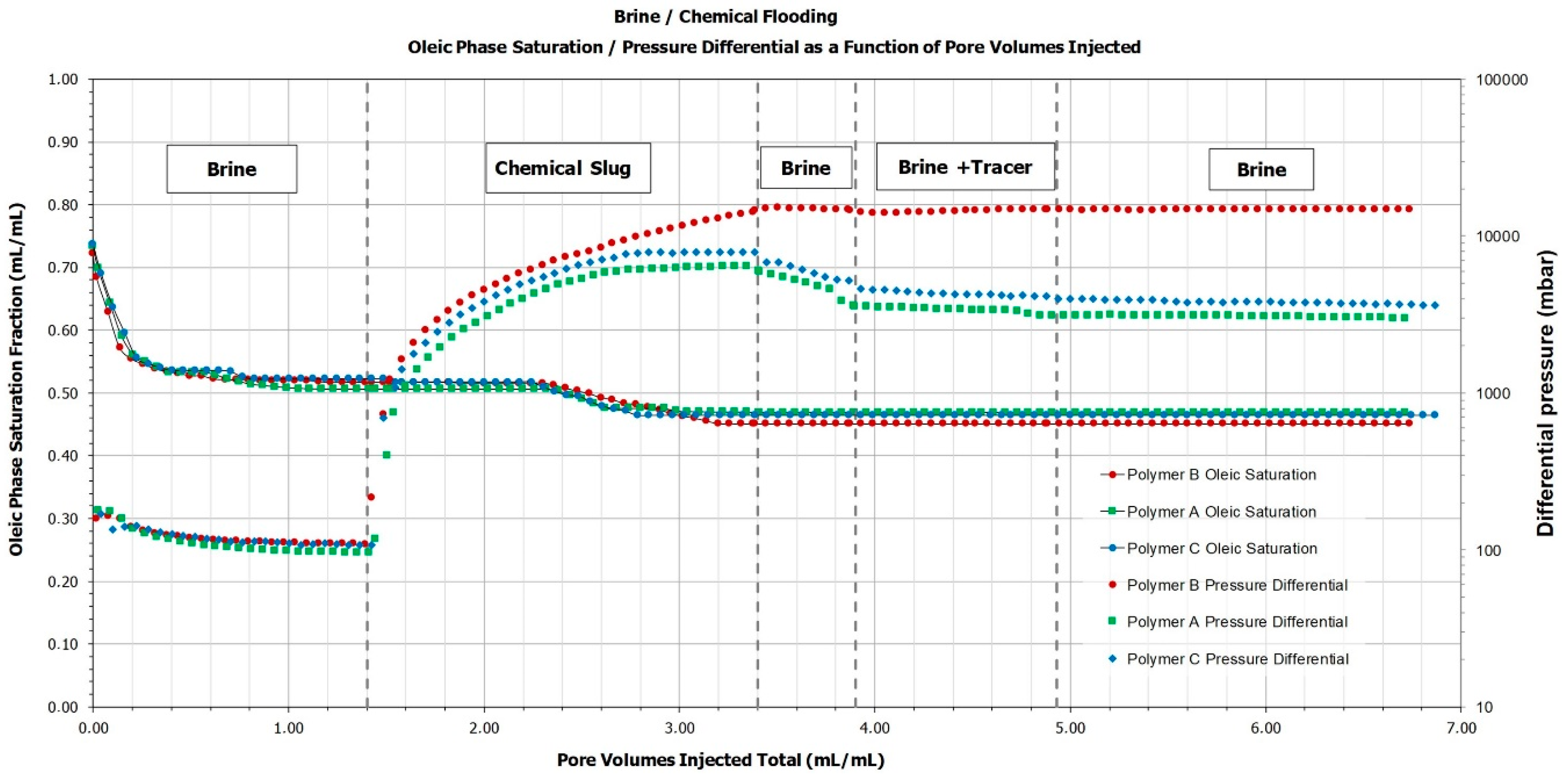
- Synthetic formation brine injection for 1.4 PV (water flooding to determine water flood recovery),
- 13.
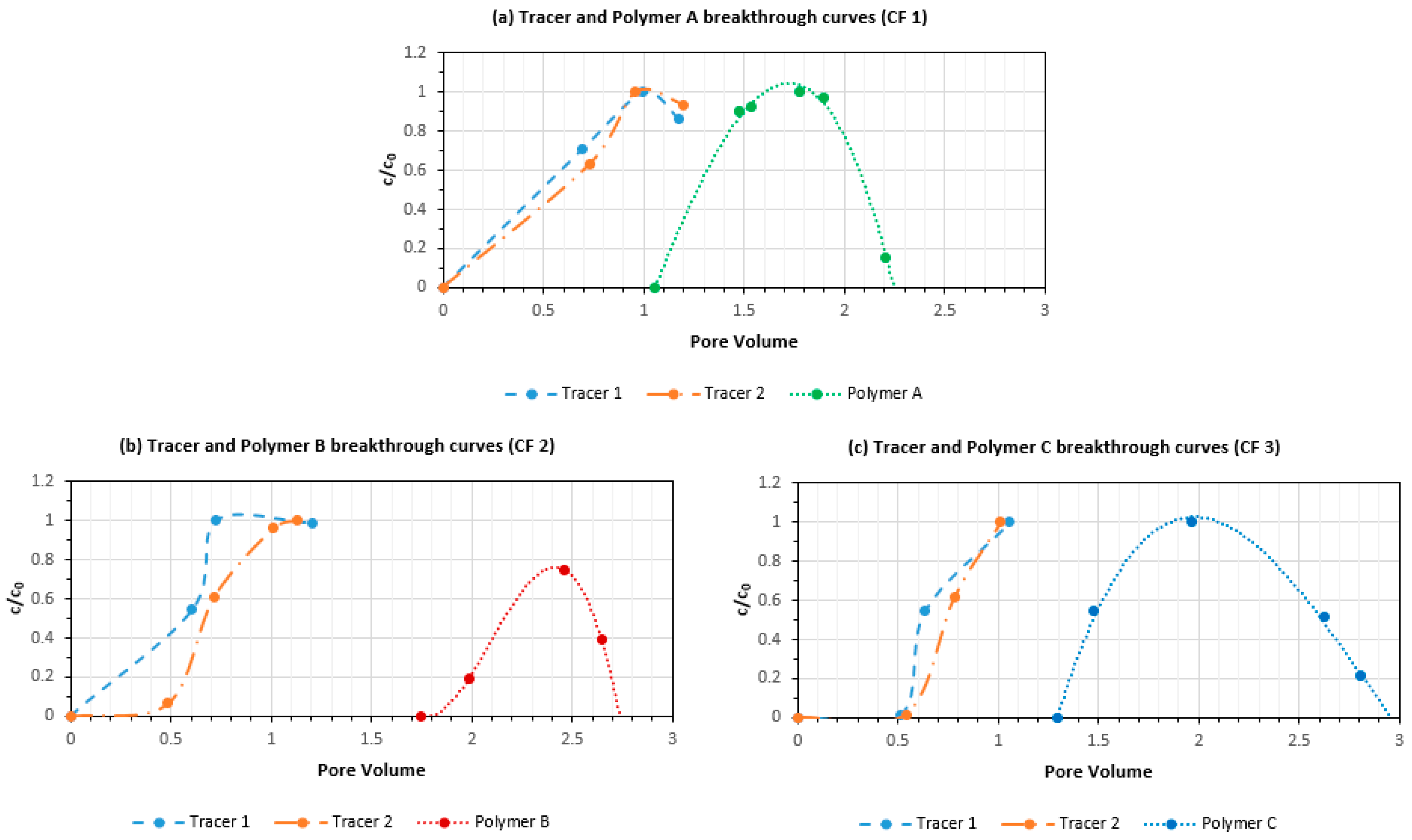
- Polymer slug with KBr tracer for 2 PV (tertiary-mode polymer flooding to determine any incremental due to polymer flooding and to determine flow contributing pore volume),
- 14.
- Synthetic formation brine for 0.5 PV (to clean the lines from polymer and/or oil),
- 15.
- Synthetic formation brine with KBr tracer for 1.0 PV (to determine flow contributing PV after polymer injection),
- 16.
- Synthetic formation brine for 2 PV (to determine RRF deep within the reservoir).
4. Results and Discussion
- Berea core water wet behaviour,
- Berea relatively high specific surface area (≈1.4364 m2/g-cores in this work)
- Anionic nature of polymers,
- Small interstitial velocities used (1 ft/d),
- Relatively small amount of pore volumes utilized in the experiment
5. Polymer Selection
- 17.
- The oil production needs to be accelerated along the flow paths by improving the mobility ratio.
- 18.
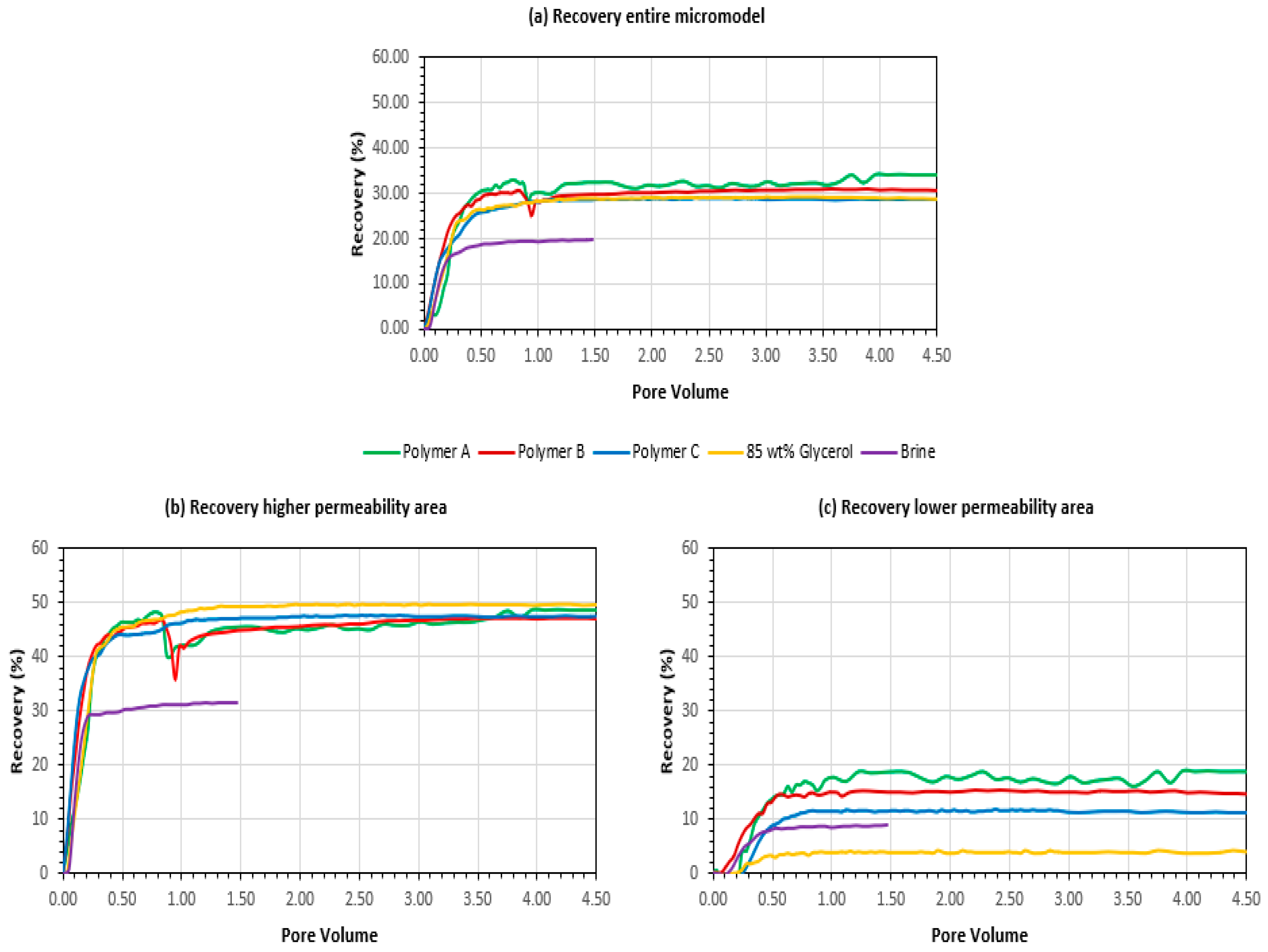
- In heterogeneous reservoirs, the polymer solutions need to be able to increase oil recovery from the various rock types.
- 19.
- The mass of polymer injected per incremental barrel of oil produced (Utility Factor) needs to be low.
- 20.
- Costs of polymers for the same incremental recovery factor need to be low.
- 21.
- The polymer solutions need to be resistant to degradation.
- 22.
- In addition, the polymers need to show good mixing (e.g., no fisheyes) and separation characteristics (produced fluids containing polymers).
6. Conclusions
- Full spectrum MWD measurement using Field-Flow Fractionation is a key in understanding polymer behavior. Polymers having a large number of heavier molecules, even though they generally require less concertation to achieve the desired viscosity have to be thoroughly evaluated in the laboratory before field application. FFF measurement of Polymer B already indicated potential injectivity issues.
- Heterogenous micromodel evaluations provided consistent data to subsequent core flood evaluations and were in alignment with FFF indications. Therefore, they can be used as a primary screening criteria of polymer injectivity and displacement efficiency. Given the relatively short time for performing such experiments, they can be used as a method of eliminating certain polymers at start of evaluations. These experiments also pointed Polymer B as an outlier.
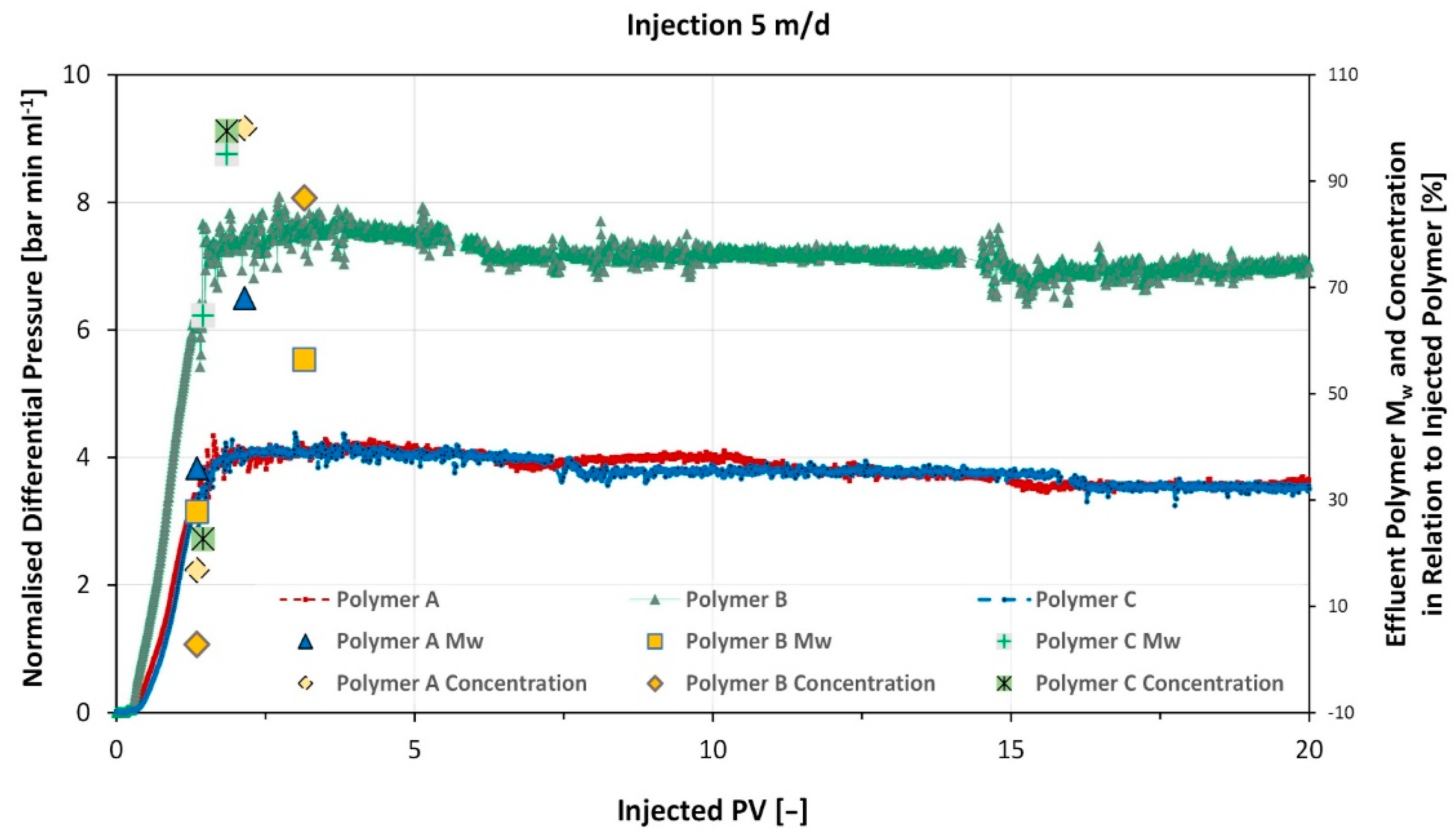
- Single-phase core floods performed at near wellbore, higher injection velocities (5 m/d) in combination of FFF showed that narrower MWD distribution polymers (polymers A and C) have less retention and better injectivity.
- Two-phase core floods performed at low, reservoir representative velocities (1 ft/d) showed that Polymer B could not be injected, with pressure response staying at high values even when chase brine is injected. Adsorption values for all tested polymers at these conditions were high, however highest were observed in the case of polymer B.
- Combination of all laboratory measurement pointed in the same direction and that is that field injection of polymer B might be risky, therefore polymer C was selected as alternative polymer. Long term field injectivity test currently ongoing with polymer C did not show any issues, thus improving project economics by having lower OPEX (polymer C base cost is less than polymer A).
- Selection of polymers needs to take near-wellbore behavior as well as sweep efficiency (along flow paths and volumetric), reservoir heterogeneity, incremental recovery, polymer retention and surface aspects into account.
Author Contributions
Funding
Institutional Review Board Statement
Data Availability Statement
Acknowledgments
Conflicts of Interest
Abbreviations
| FFF | Field-Flow Fractionation |
| HPAM | high molecular weight polyacrylamide polymers |
| MALS | Multi Angle Light Scattering |
| MWD | Molecular Weight Distribution |
| NPV | Net Present Value |
| OPEX | Operating Expenditures |
| PV | Pore Volume |
| RF | Resistance Factor |
| RRF | Residual Resistance Factor |
| TDS | Total Dissolved Solids |
| UF | Utility Factor |
References
- Delamaide, E. Is Chemical EOR Finally Coming of Age? In Proceedings of the SPE Asia Pacific Oil & Gas Conference and Exhibition, Virtual, 17–19 November 2020. [Google Scholar] [CrossRef]
- Anand, A.; Al Sulaimani, H.; Riyami, O.; AlKindi, A. Success and Challenges in Ongoing Field Scale Polymer Flood in Sultanate of Oman-A Holistic Reservoir Simulation Case Study for Polymer Flood Performance Analysis and Prediction. In Proceedings of the SPE EOR Conference at Oil and Gas West Asia, Muscat, Oman, 26–28 March 2018. [Google Scholar] [CrossRef]
- Delamaide, E.; Bazin, B.; Rousseau, D.; Degre, G. Chemical EOR for Heavy Oil: The Canadian Experience. In Proceedings of the SPE EOR Conference at Oil and Gas West Asia, Muscat, Oman, 31 March–2 April 2014. [Google Scholar] [CrossRef]
- Delamaide, E.; Zaitoun, A.; Renard, G.; Tabary, R. Pelican Lake Field: First Successful Application of Polymer Flooding in a Heavy Oil Reservoir. In Proceedings of the SPE Enhanced Oil Recovery Conference, Kuala Lumpur, Malaysia, 2–4 July 2013. [Google Scholar] [CrossRef]
- Gao, S.; He, Y.; Zhu, Y.; Han, P.; Peng, S.; Liu, X. Associated Polymer ASP Flooding Scheme Optimization Design and Field Test after Polymer Flooding in Daqing Oilfield. In Proceedings of the SPE Improved Oil Recovery Conference, Virtual, 31 August–4 September 2020. [Google Scholar] [CrossRef]
- Juri, J.E.; Ruiz, A.M.; Pedersen, G.; Pagliero, P.; Blanco, H.; Eguia, V.; Vazquez, P.; Bernhardt, C.; Schein, F.; Villarroel, G.; et al. Grimbeek2: First Successful Application Polymer Flooding in Multilayer Reservoir at YPF. Interpretation of Polymer Flooding Response. In Proceedings of the SPE Latin America and Caribbean Petroleum Engineering Conference, Buenos Aires, Argentina, 17–19 May 2017. [Google Scholar] [CrossRef]
- Pan, G.; Zhang, L.; Huang, J.; Li, H.; Qu, J. Twelve Years Field Applications of Offshore Heavy Oil Polymer Flooding from Continuous Injection to Alternate Injection of Polymer-Water. In Proceedings of the Offshore Technology Conference Asia, Kuala Lumpur, Malaysia, 2–6 November 2020. [Google Scholar] [CrossRef]
- Sieberer, M.; Clemens, T.; Peisker, J.; Ofori, S. Polymer-Flood Field Implementation: Pattern Configuration and Horizontal vs. Vertical Wells. SPE Reserv. Eval. Eng. 2019, 22, 577–596. [Google Scholar] [CrossRef]
- Rock, A.; Hincapie, R.E.; Tahir, M.; Langanke, N.; Ganzer, L. On the Role of Polymer Viscoelasticity in Enhanced Oil Recovery: Extensive Laboratory Data and Review. Polymers 2020, 12, 2276. [Google Scholar] [CrossRef] [PubMed]
- Seright, R.S.; Fan, T.; Wavrik, K.; de Carvalho Balaban, R. New Insights Into Polymer Rheology in Porous Media. SPE J. 2010, 16, 35–42. [Google Scholar] [CrossRef]
- Stavland, A.; Jonsbråten, H.C.; Lohne, A.; Moen, A.; Giske, N.H. Polymer Flooding–Flow Properties in Porous Media Versus Rheological Parameters. In Proceedings of the SPE EUROPEC/EAGE Annual Conference and Exhibition, Barcelona, Spain, 14–17 June 2010. [Google Scholar] [CrossRef]
- Chauveteau, G. Molecular Interpretation of Several Different Properties of Flow of Coiled Polymer Solutions Through Porous Media in Oil Recovery Conditions. In Proceedings of the SPE Annual Technical Conference and Exhibition, San Antonio, TX, USA, 4 October 1981. [Google Scholar] [CrossRef]
- Sieberer, M.; Jamek, K.; Clemens, T. Polymer-Flooding Economics, From Pilot to Field Implementation. SPE Econ. Manag. 2017, 9, 51–60. [Google Scholar] [CrossRef]
- Guo, H. How to Select Polymer Molecular Weight and Concentration to Avoid Blocking in Polymer Flooding? In Proceedings of the SPE Symposium: Production Enhancement and Cost Optimisation, Kuala Lumpur, Malaysia, 7–8 November 2017. [Google Scholar] [CrossRef]
- Zong, J.; Guo, H.; He, S.; Song, K.; Li, X.; Huang, F.; Chen, J.; Fu, H.; Wang, Z.; Song, K.; et al. Polymer Injectivity Learned from 20 Years’ Polymer Flooding Field Practices. In Proceedings of the EAGE IOR 2021 Conference, Online, 19–22 April 2021. [Google Scholar] [CrossRef]
- Guo, H.; Lyu, X.; Xu, Y.; Liu, S.; Zhang, Y.; Zhao, F.; Wang, Z.; Tang, E.; Yang, Z.; Liu, H.; et al. Recent advanced of Polymer Flooding in China. In Proceedings of the SPE Conference at Oman Petroleum & Energy Show, Muscat, Omant, 9–11 March 2020. [Google Scholar] [CrossRef]
- Zhong, H.; He, Y.; Yang, E.; Bi, Y.; Yang, T. Modeling of microflow during viscoelastic polymer flooding in heterogenous reservoirs of Daqing Oilfield. J. Pet. Sci. Eng. 2022, 210, 110091. [Google Scholar] [CrossRef]
- Xiaoqin, Z. Application of Polymer Flooding with High Molecular Weight and Concentration in Heterogeneous Reservoirs. In Proceedings of the SPE Enhanced Oil Recovery Conference, Kuala Lumpur, Malaysia, 19–21 July 2011. [Google Scholar] [CrossRef]
- Al-Hashmi, A.R.; Divers, T.; Al-Maamari, R.S.; Favero, C.; Thomas, A. Improving Polymer Flooding Efficiency in Oman Oil Fields. In Proceedings of the SPE EOR Conference at Oil and Gas West Asia, Muscat, Oman, 21–23 March 2016. [Google Scholar] [CrossRef]
- Marx, M.; Grottendorfer, S.; Krenn, C.; Grillneder, R. Overcoming Back-Produced Polymer Challenges-Development of an Advanced and Economic Filtration Technology for CEOR Application. In Proceedings of the SPE Russian Petroleum Technology Conference, Virtual, 26–29 October 2020. [Google Scholar] [CrossRef]
- Davidescu, B.G.; Bayerl, M.; Puls, C.; Clemens, T. Horizontal Versus Vertical Wells: Assessment of Sweep Efficiency in a Multi-Layered Reservoir Based on Consecutive Inter-Well Tracer Tests-A Comparison between Water Injection and Polymer EOR. In Proceedings of the SPE Europec Featured at 82nd EAGE Conference and Exhibition, Amsterdam, The Netherlands, 18–21 October 2021. [Google Scholar] [CrossRef]
- Lüftenegger, M.; Kadnar, R.; Puls, C.; Clemens, T. Operational Challenges and Monitoring of a Polymer Pilot, Matzen Field, Austria. SPE Prod. Oper. 2016, 31, 228–237. [Google Scholar] [CrossRef]
- Divers, T.; Gaillard, N.; Bataille, S.; Thomas, A.; Favéro, C. Successful Polymer Selection for CEOR: Brine Hardness and Mechanical Degradation Considerations. In Proceedings of the SPE Oil and Gas India Conference and Exhibition, Mumbai, India, 4 April 2017. [Google Scholar] [CrossRef]
- Bolton, H.P.; Carter, W.H.; Kamdar, R.S.; Nute, A.J. Selection of Polymers for the Control of Mobility and Permeability Variation at Richfield East Dome Unit, Orange County, California. In Proceedings of the SPE California Regional Meeting, Los Angeles, CA, USA, 14 April 1980. [Google Scholar] [CrossRef]
- Thomas, A. Essentials of Polymer Flooding Technique; John Wiley & Sons Ltd. Wiley Library: Hoboken, NJ, USA, 2019; ISBN 9781119537618. [Google Scholar] [CrossRef]
- Schumi, B.; Clemens, T.; Wegner, J.; Ganzer, L.; Kaiser, A.; Hincapie, R.E. Alkali/Cosolvent/Polymer Flooding of High-TAN Oil: Using Phase Experiments, Micromodels, and Corefloods for Injection-Agent Selection. SPE Reserv. Eval. Eng. 2020, 23, 463–478. [Google Scholar] [CrossRef]
- Wegner, J.; Ganzer, L. Rock-on-a-Chip Devices for High p, T Conditions and Wettability Control for the Screening of EOR Chemicals. In Proceedings of the Paper SPE 185820 presented at the SPE Europec Featured at the 79th EAGE Conference and Exhibition, Paris, France, 12–15 June 2017. [Google Scholar] [CrossRef]
- Gaol, C.L.; Wegner, J.; Ganzer, L. Real structure micromodels based on reservoir rocks for enhanced oil recovery (EOR) applications. Lab Chip 2020, 20, 2197–2208. [Google Scholar] [CrossRef] [PubMed]
- Hu, J.; Li, A.; Memon, A. Experimental Investigation of Polymer Enhanced Oil Recovery under Different Injection Modes. ACS Omega 2020, 5, 31069–31075. [Google Scholar] [CrossRef] [PubMed]
- Seright, R.S.; Fan, T.; Wavrik, K.; de Balaban, R. New Insights into Polymer Rheology in Porous Media. Paper presented at the SPE Improved Oil Recovery Symposium, Tulsa, Oklahoma, USA, 23 April 2010. [Google Scholar] [CrossRef]
- Benincasa, M.A.; Giddings, J.C. Separation and molecular weight distribution of anionic and cationic water-soluble polymers by flow field-flow fractionation. Anal. Chem. 1992, 64, 790–798. [Google Scholar] [CrossRef]
- Steindl, J.; Hincapie, R.E.; Borovina, A.; Puls, C.; Badstoeber, J.; Heinzmann, G.; Clemens, T. Improved Enhanced Oil Recovery Polymer Selection Using Field-Flow Fractionation. SPE Res. Eval. Eng. 2022, 25, 319–330. [Google Scholar] [CrossRef]
- Clemens, T.; Lüftenegger, M.; Laoroongroj, A.; Kadnar, R.; Puls, C. The Use of Tracer Data To Determine Polymer-Flooding Effects in a Heterogeneous Reservoir, 8 Torton Horizon Reservoir, Matzen Field, Austra. SPE-174349-PA. SPE Reserv. Eval. Eng. 2016, 19, 655–663. [Google Scholar] [CrossRef]
- van den Hoek, P.J.; Al-Masfry, R.A.; Zwarts, D.; Jansen, J.D.; Hustedt, B.; van Schijndel, L. Optimizing Recovery for Waterflooding Under Dynamic Induced Fracturing Conditions. SPE Res. Eval. Eng. 2009, 12, 671–682. [Google Scholar] [CrossRef]
- Moe Soe Let, K.P.; Manichand, R.N.; Seright, R.S. Polymer Flooding a ~500-Cp Oil. In Proceedings of the Eighteenth SPE Improved Oil Recovery Symposium, Tulsa, OK, USA, 14–18 April 2012. SPE-154567-MS. [Google Scholar] [CrossRef]
- Zechner, M.; Clemens, T.; Suri, A.; Sharma, M.M. Simulation of Polymer Injection Under Fracturing Conditions–An Injectivity Pilot in the Matzen Field, Austria. SPE 169043-PA. SPE Reserv. Eval. Eng. 2015, 18, 236–249. [Google Scholar] [CrossRef]
- Hincapie, R.E.; Ganzer, L. Assessment of Polymer Injectivity with Regards to Viscoelasticity: Lab Evaluations towards Better Field Operations. In Proceedings of the EUROPEC 2015, Madrid, Spain, 1–4 June 2015. [Google Scholar] [CrossRef]
- Chiotoroiu, M.-M.; Clemens, T.; Zechner, M.; Hwang, J.; Sharma, M.M.; Thiele, M. Risk Assessment and Simulation of Injectivity Decline Under Uncertainty. SPE 195499-PA. SPE Prod. Oper. 2020, 35, 308–319. [Google Scholar] [CrossRef]
- Cheng, J.; Wie, J.; Song, K.; Peihui, H. Study on Remaining Oil Distribution after Polymer Injection. In Proceedings of the Paper SPE 133808 presented at the SPE Annual Technical Conference and Exhibition, Florence, Italy, 19–22 September 2010. [Google Scholar] [CrossRef]
- Clemens, T.; Abdev, J.; Thiele, M.R. Improved Polymer-Flood Management Using Streamlines. SPE Res. Eval. Eng. 2011, 14, 171–181. [Google Scholar] [CrossRef]
- Choudhuri, B.; Thakuria, C.; Belushi, A.A.; Nurzaman, Z.; Al Hashmi, K.; Batycky, R. Optimization of a Large Polymer Flood With Full-Field Streamline Simulation. SPE 169746-PA. SPE Reserv. Eval. Eng. 2015, 18, 318–328. [Google Scholar] [CrossRef]
- Sieberer, M.; Clemens, T. Hydrocarbon Field (Re-)Development as Markov Decision Process. SPE Res. Eval. Eng. 2022, 25, 273–286. [Google Scholar] [CrossRef]


| Property | |
|---|---|
| Reservoir | 8 TH |
| Well | Schönkirchen S85 |
| TAN [mg KOH/g] | 2.14 |
| Saturates [%] | 39 |
| Aromatics [%] | 42 |
| Resins [%] | 16 |
| Asphaltene [%] | 3 |
| Saponifiable Acids [µmol/g] | 41 |
| µ at Res. Cond. [mPa.s] | 20.0 |
| Polymer | Concentration [ppm] | Temperature [°C] | Viscosity [mPa.s] | Experiment Purpose |
|---|---|---|---|---|
| A | 1850 | 30 | 25 | Single-phase injectivity with FFF |
| 2000 | 49 | 23 | Two-phase (Core floods and micromodels) | |
| B | 1400 | 30 | 25 | Single-phase injectivity with FFF |
| 1700 | 49 | 23 | Two-phase (Core floods and micromodels) | |
| C | 1850 | 30 | 26 | Single-phase injectivity with FFF |
| 2000 | 49 | 25 | Two-phase (Core floods and micromodels) | |
| Glycerol | 850,000 | 49 | 24 | Two-phase (baseline for micromodel) |
| Polymer | Mn, [MDa] | Mw, [MDa] | Đ, [-] | rg, [nm] |
|---|---|---|---|---|
| A | 6.7 ± 2.9% | 52 ± 2.5% | 7.76 | 358 ± 2.1% |
| B | 112 ± 20.4% | 619 ± 2.3% | 5.53 | 1094 ± 1.6% |
| C | 6.5 ± 7.1% | 10 ± 4.9% | 1.52 | 206 ± 4.5% |
| Polymer | RF [-] | RRF [-] |
|---|---|---|
| A | 82 | 18 |
| B | 153 | 22 |
| C | 86 | 23 |
| Parameter | Unit | Polymer A | Polymer B | Polymer C |
|---|---|---|---|---|
| Length/Diameter | cm | 30.25/3.81 | 30.15/3.81 | 30.10/3.81 |
| Porosity | % | 22 | 23 | 22 |
| Dry mass | g | 705.35 | 703.42 | 703.13 |
| kw/ko at Swi | mD | 297/232 | 278/216 | 279/249 |
| So initial | % | 73 | 72 | 73 |
| So after brine flood | % | 51 | 52 | 52 |
| So after polymer flood | % | 47 | 45 | 46.5 |
| Polymer induced saturation change | % | 4 | 7 | 5.5 |
| Max ΔP from Polymer Injection | bar | 6.5 | 15 | 7.9 |
| Maximum Measured RF | bar/bar | 67 | 140 | 74 |
| Lowest Measured RRF | bar/bar | 31 | 129 | 34 |
| Adsorption | µg/g | 202 | 293 | 177 |
Publisher’s Note: MDPI stays neutral with regard to jurisdictional claims in published maps and institutional affiliations. |
© 2022 by the authors. Licensee MDPI, Basel, Switzerland. This article is an open access article distributed under the terms and conditions of the Creative Commons Attribution (CC BY) license (https://creativecommons.org/licenses/by/4.0/).
Share and Cite
Borovina, A.; Hincapie, R.E.; Clemens, T.; Hoffmann, E.; Wegner, J. Selecting EOR Polymers through Combined Approaches—A Case for Flooding in a Heterogenous Reservoir. Polymers 2022, 14, 5514. https://doi.org/10.3390/polym14245514
Borovina A, Hincapie RE, Clemens T, Hoffmann E, Wegner J. Selecting EOR Polymers through Combined Approaches—A Case for Flooding in a Heterogenous Reservoir. Polymers. 2022; 14(24):5514. https://doi.org/10.3390/polym14245514
Chicago/Turabian StyleBorovina, Ante, Rafael E. Hincapie, Torsten Clemens, Eugen Hoffmann, and Jonas Wegner. 2022. "Selecting EOR Polymers through Combined Approaches—A Case for Flooding in a Heterogenous Reservoir" Polymers 14, no. 24: 5514. https://doi.org/10.3390/polym14245514
APA StyleBorovina, A., Hincapie, R. E., Clemens, T., Hoffmann, E., & Wegner, J. (2022). Selecting EOR Polymers through Combined Approaches—A Case for Flooding in a Heterogenous Reservoir. Polymers, 14(24), 5514. https://doi.org/10.3390/polym14245514