
A Hybrid SVR-Based Prediction Model for the Interfacial Bond Strength of Externally Bonded FRP Laminates on Grooves with Concrete Prisms

 , , , , , ,
  and
and
Abstract
:1. Introduction

2. Methodology
2.1. Overview of Optimization Algorithms
2.2. Support Vector Machines (SVMs)
2.3. Particle Swarm Optimization (PSO)
2.4. Grey Wolf Optimization (GWO)
2.5. Equilibrium Optimizer (EO)
2.6. Harris Hawks Optimization (HHO)
2.7. Slime Mold Algorithm (SMA)
2.8. Hybridization Procedure for SVMs and OAs
3. Data Processing and Analysis
3.1. Descriptive Statistics and Statistical Analysis
3.2. Performance Parameters
4. Results and Discussion
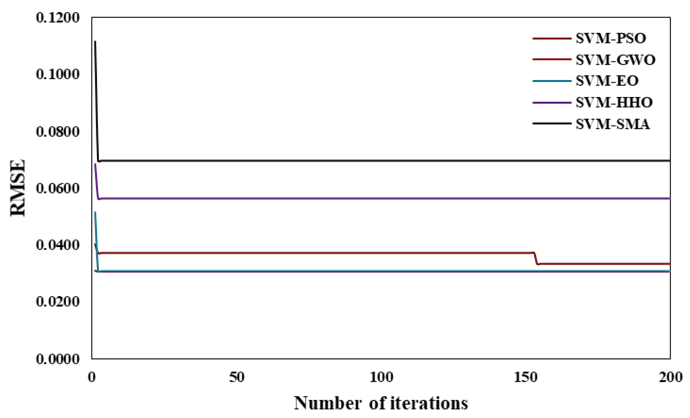
4.1. Parametric Configuration
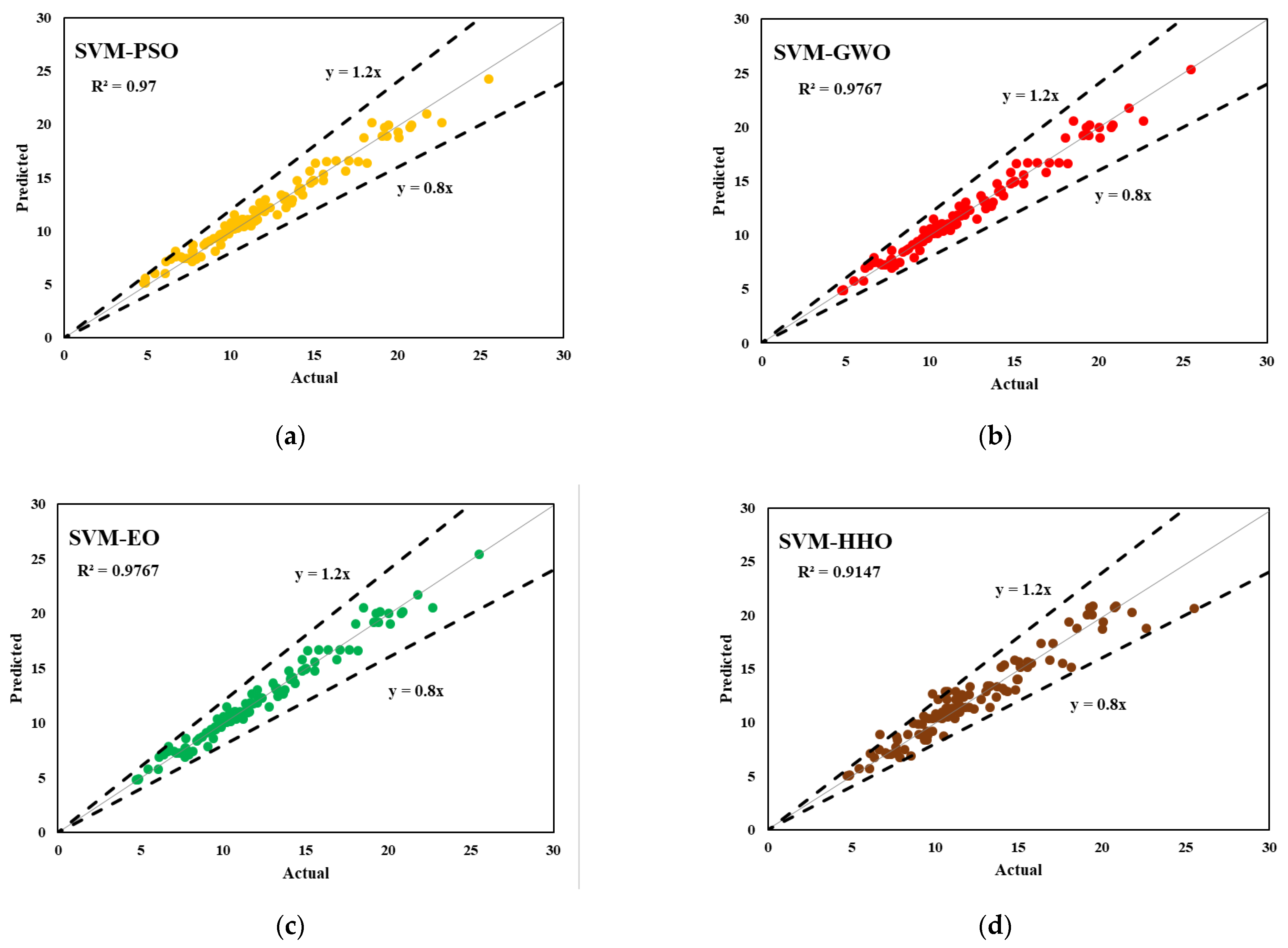
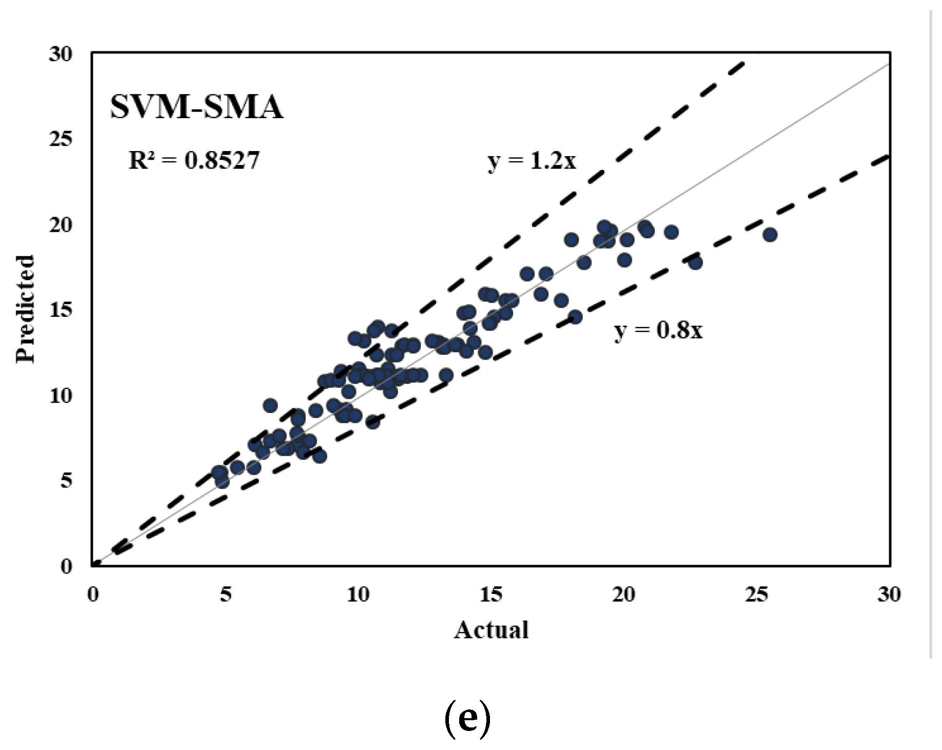
4.2. Model Performance
4.3. Taylor Diagrams
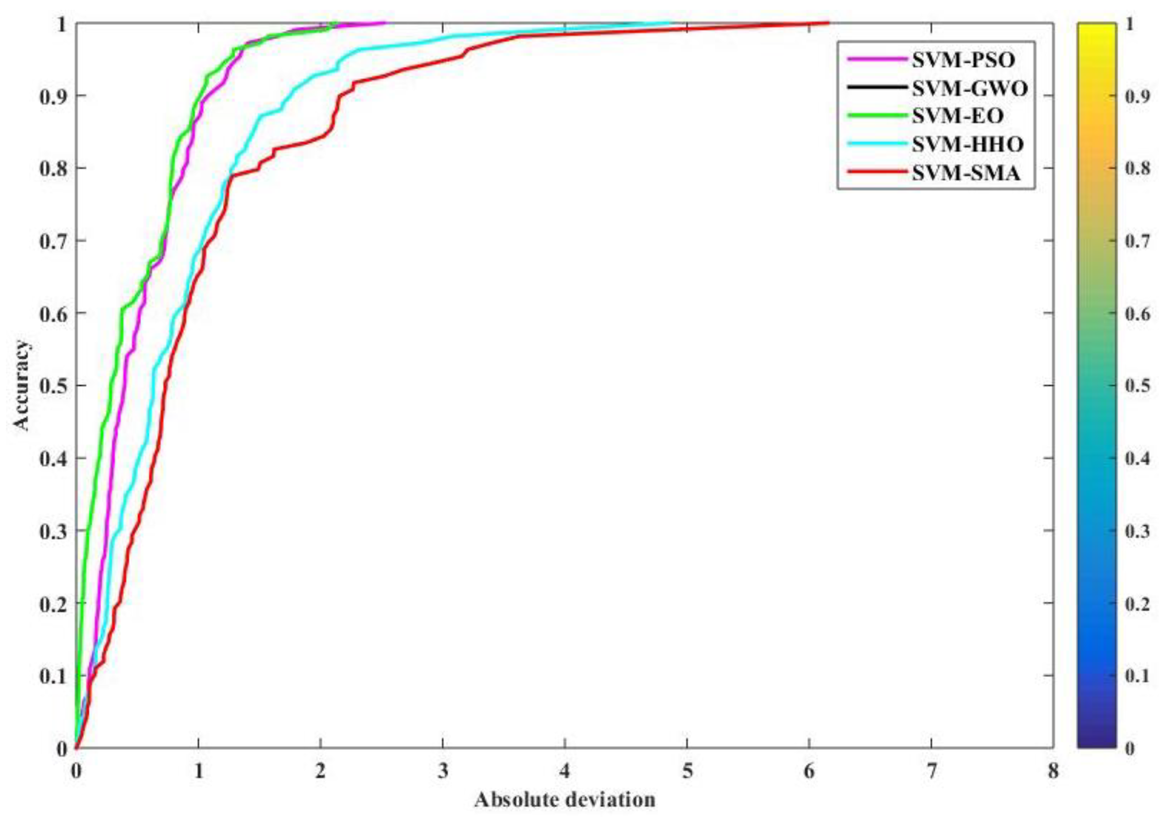
4.4. Regression Error Characteristic Curve
5. Conclusions
Author Contributions
Funding
Institutional Review Board Statement
Informed Consent Statement
Data Availability Statement
Acknowledgments
Conflicts of Interest
References
- Liberati, E.A.P.; Nogueira, C.G.; Leonel, E.D.; Chateauneuf, A. Nonlinear formulation based on FEM, Mazars damage criterion and Fick’s law applied to failure assessment of reinforced concrete structures subjected to chloride ingress and reinforcements corrosion. Eng. Fail. Anal. 2014, 46, 247–268. [Google Scholar] [CrossRef]
- Siddika, A.; al Mamun, M.A.; Ferdous, W.; Alyousef, R. Performances, challenges and opportunities in strengthening reinforced concrete structures by using FRPs—A state-of-the-art review. Eng. Fail. Anal. 2020, 111, 104480. [Google Scholar] [CrossRef]
- Yang, J.; Haghani, R.; Blanksvärd, T.; Lundgren, K. Experimental study of FRP-strengthened concrete beams with corroded reinforcement. Constr. Build. Mater. 2021, 301, 124076. [Google Scholar] [CrossRef]
- Panahi, M.; Zareei, S.A.; Izadi, A. Flexural strengthening of reinforced concrete beams through externally bonded FRP sheets and near surface mounted FRP bars. Case Stud. Constr. Mater. 2021, 15, e00601. [Google Scholar] [CrossRef]
- Kotynia, R.; Oller, E.; Marí, A.; Kaszubska, M. Efficiency of shear strengthening of RC beams with externally bonded FRP materials—State-of-the-art in the experimental tests. Compos. Struct. 2021, 267, 113891. [Google Scholar] [CrossRef]
- Abedini, M.; Zhang, C. Dynamic performance of concrete columns retrofitted with FRP using segment pressure technique. Compos. Struct. 2021, 260, 113473. [Google Scholar] [CrossRef]
- Hadi, M.N.S. Behaviour of FRP strengthened concrete columns under eccentric compression loading. Compos. Struct. 2007, 77, 92–96. [Google Scholar] [CrossRef] [Green Version]
- Tafsirojjaman, T.; Fawzia, S.; Thambiratnam, D.P.; Zhao, X.L. FRP strengthened SHS beam-column connection under monotonic and large-deformation cyclic loading. Thin-Walled Struct. 2021, 161, 107518. [Google Scholar] [CrossRef]
- Lee, W.T.; Chiou, Y.J.; Shih, M.H. Reinforced concrete beam-column joint strengthened with carbon fiber reinforced polymer. Compos. Struct. 2010, 92, 48–60. [Google Scholar] [CrossRef]
- Wu, Y.-F.; Jiang, C. Quantification of Bond-Slip Relationship for Externally Bonded FRP-to-Concrete Joints. J. Compos. Constr. 2013, 17, 673–686. [Google Scholar] [CrossRef]
- Fathelbab, F.A.; Ramadan, M.S.; Al-Tantawy, A. Strengthening of RC bridge slabs using CFRP sheets. Alex. Eng. J. 2014, 53, 843–854. [Google Scholar] [CrossRef] [Green Version]
- Xian, G.; Guo, R.; Li, C. Combined effects of sustained bending loading, water immersion and fiber hybrid mode on the mechanical properties of carbon/glass fiber reinforced polymer composite. Compos. Struct. 2021, 281, 115060. [Google Scholar] [CrossRef]
- Ding, J.; Cheng, L.; Chen, X.; Chen, C.; Liu, K. A review on ultra-high cycle fatigue of CFRP. Compos. Struct. 2021, 256, 113058. [Google Scholar] [CrossRef]
- Guo, R.; Xian, G.; Li, F.; Li, C.; Hong, B. Hygrothermal resistance of pultruded carbon, glass and carbon/glass hybrid fiber reinforced epoxy composites. Constr. Build. Mater. 2021, 315, 125710. [Google Scholar] [CrossRef]
- Zhang, S.S.; Yu, T.; Chen, G.M. Reinforced concrete beams strengthened in flexure with near-surface mounted (NSM) CFRP strips: Current status and research needs. Compos. Part B Eng. 2017, 131, 30–42. [Google Scholar] [CrossRef] [Green Version]
- Ghorbani, M.; Mostofinejad, D.; Hosseini, A. Experimental investigation into bond behavior of FRP-to-concrete under mixed-mode I/II loading. Constr. Build. Mater. 2017, 132, 303–312. [Google Scholar] [CrossRef]
- Bakay, R.; Shrive, N.G.; Sayed-Ahmed, E.Y. Bond Strength of FRP Laminates to Concrete: State-of-the-Art Review. Electron. J. Struct. Eng. 2009, 9, 45–61. [Google Scholar]
- Teng, T.; Chen, J.; Yu, J.-F. FRP-Strengthened RC Structures; John Wiley & Sons Ltd.: Hoboken, NJ, USA, 2002. [Google Scholar]
- Nguyen, B.D.M.; Chan, T.K.; Cheong, H.K. Brittle Failure and Bond Development Length of Cfrp-Concrete Beams. J. Compos. Constr. 2001, 5, 12–17. [Google Scholar] [CrossRef]
- Lu, Z.; Xian, G.; Li, H. Effects of exposure to elevated temperatures and subsequent immersion in water or alkaline solution on the mechanical properties of pultruded BFRP plates. Compos. Part B Eng. 2015, 77, 421–430. [Google Scholar] [CrossRef]
- Smith, S.T.; Teng, J.G. FRP-strengthened RC beams. I: Review of debonding strength models. Eng. Struct. 2002, 24, 385–395. [Google Scholar] [CrossRef]
- Wan, B.; Jiang, C.; Wu, Y.F. Effect of defects in externally bonded FRP reinforced concrete. Constr. Build. Mater. 2018, 172, 63–76. [Google Scholar] [CrossRef]
- Chajes, M.J.; Finch, W.W.; Januszka, T.F.; Thomson, T.A. Bond and force transfer of composite material plates bonded to concrete. ACI Struct. J. 1996, 93, 208–217. [Google Scholar] [CrossRef]
- Jiang, C.; Wan, B.; Wu, Y.F.; Omboko, J. Epoxy interlocking: A novel approach to enhance FRP-to-concrete bond behavior. Constr. Build. Mater. 2018, 193, 643–653. [Google Scholar] [CrossRef]
- Kishore, K.; Gupta, N. Mechanical characterization and assessment of composite geopolymer concrete. Mater. Today Proc. 2021, 44, 58–62. [Google Scholar] [CrossRef]
- Tiwari, P.K.; Sharma, P.; Sharma, N.; Verma, M.; Rohitash. An experimental investigation on metakaoline GGBS based concrete with recycled coarse aggregate. Mater. Today Proc. 2020, 43, 1025–1030. [Google Scholar] [CrossRef]
- Parashar, A.K.; Gupta, N.; Kishore, K.; Nagar, P.A. An experimental investigation on mechanical properties of calcined clay concrete embedded with bacillus subtilis. Mater. Today Proc. 2021, 44, 129–134. [Google Scholar] [CrossRef]
- Mostofinejad, D.; Mahmoudabadi, E. Grooving as Alternative Method of Surface Preparation to Postpone Debonding of FRP Laminates in Concrete Beams. J. Compos. Constr. 2010, 14, 804–811. [Google Scholar] [CrossRef]
- Bencardino, F.; Condello, A.; Ashour, A.F. Single-lap shear bond tests on Steel Reinforced Geopolymeric Matrix-concrete joints. Compos. Part B Eng. 2017, 110, 62–71. [Google Scholar] [CrossRef] [Green Version]
- Mofrad, M.H.; Mostofinejad, D.; Hosseini, A. A generic non-linear bond-slip model for CFRP composites bonded to concrete substrate using EBR and EBROG techniques. Compos. Struct. 2019, 220, 31–44. [Google Scholar] [CrossRef]
- Al-Jaberi, Z.; Myers, J.J.; Chandrashekhara, K. Effect of direct service temperature exposure on the bond behavior between advanced composites and CMU using NSM and EB techniques. Compos. Struct. 2019, 211, 63–75. [Google Scholar] [CrossRef]
- Yuan, H.; Teng, J.G.; Seracino, R.; Wu, Z.S.; Yao, J. Full-range behavior of FRP-to-concrete bonded joints. Eng. Struct. 2004, 26, 553–565. [Google Scholar] [CrossRef]
- Figiel, Ł.; Kamiński, M. Numerical probabilistic approach to sensitivity analysis in a fatigue delamination problem of a two layer composite. Appl. Math. Comput. 2009, 209, 75–90. [Google Scholar] [CrossRef]
- Carrara, P.; Ferretti, D. A finite-difference model with mixed interface laws for shear tests of FRP plates bonded to concrete. Compos. Part B Eng. 2013, 54, 329–342. [Google Scholar] [CrossRef]
- Bardhan, A.; Samui, P.; Ghosh, K.; Gandomi, A.H.; Bhattacharyya, S. ELM-based adaptive neuro swarm intelligence techniques for predicting the California bearing ratio of soils in soaked conditions. Appl. Soft Comput. 2021, 110, 107595. [Google Scholar] [CrossRef]
- Biswas, R.; Samui, P.; Rai, B. Determination of compressive strength using relevance vector machine and emotional neural network. Asian J. Civ. Eng. 2019, 20, 1109–1118. [Google Scholar] [CrossRef]
- Kumar, S.; Rai, B.; Biswas, R.; Samui, P.; Kim, D. Prediction of rapid chloride permeability of self-compacting concrete using Multivariate Adaptive Regression Spline and Minimax Probability Machine Regression. J. Build. Eng. 2020, 32, 101490. [Google Scholar] [CrossRef]
- Biswas, R.; Rai, B. Effect of cementing efficiency factor on the mechanical properties of concrete incorporating silica fume. J. Struct. Integr. Maint. 2020, 5, 190–203. [Google Scholar] [CrossRef]
- Biswas, R.; Rai, B.; Samui, P.; Roy, S.S. Estimating concrete compressive strength using MARS, LSSVM and GP. Eng. J. 2020, 24, 41–52. [Google Scholar] [CrossRef]
- Biswas, R.; Bardhan, A.; Samui, P.; Rai, B.; Nayak, S.; Armaghani, D.J. Efficient soft computing techniques for the prediction of compressive strength of geopolymer concrete. Comput. Concr. 2021, 28, 221–232. [Google Scholar] [CrossRef]
- Khan, M.A.; Memon, S.A.; Farooq, F.; Javed, M.F.; Aslam, F.; Alyousef, R. Compressive Strength of Fly-Ash-Based Geopolymer Concrete by Gene Expression Programming and Random Forest. Adv. Civ. Eng. 2021, 2021, 6618407. [Google Scholar] [CrossRef]
- Khan, M.I.; Sutanto, M.H.; Khan, K.; Iqbal, M.; Bin Napiah, M.; Zoorob, S.E.; Klemeš, J.J.; Bokhari, A.; Rafiq, W. Effective use of recycled waste PET in cementitious grouts for developing sustainable semi-flexible pavement surfacing using artificial neural network (ANN). J. Clean. Prod. 2022, 340, 130840. [Google Scholar] [CrossRef]
- Iqbal, M.; Zhang, D.; Jalal, F.E.; Javed, M.F. Computational AI prediction models for residual tensile strength of GFRP bars aged in the alkaline concrete environment. Ocean. Eng. 2021, 232, 109134. [Google Scholar] [CrossRef]
- Iqbal, M.; Zhao, Q.; Zhang, D.; Jalal, F.E.; Jamal, A. Evaluation of tensile strength degradation of GFRP rebars in harsh alkaline conditions using non-linear genetic-based models. Mater. Struct. Mater. Constr. 2021, 54, 190. [Google Scholar] [CrossRef]
- Jalal, F.E.; Xu, Y.; Iqbal, M.; Jamhiri, B.; Javed, M.F. Predicting the compaction characteristics of expansive soils using two genetic programming-based algorithms. Transp. Geotech. 2021, 30, 100608. [Google Scholar] [CrossRef]
- Aamir, M.; Tolouei-Rad, M.; Vafadar, A.; Raja, M.N.A.; Giasin, K. Performance analysis of multi-spindle drilling of Al2024 with TiN and TiCN coated drills using experimental and artificial neural networks technique. Appl. Sci. 2020, 10, 8633. [Google Scholar] [CrossRef]
- Khan, M.U.A.; Shukla, S.K.; Raja, M.N.A. Soil–conduit interaction: An artificial intelligence application for reinforced concrete and corrugated steel conduits. Neural Comput. Appl. 2021, 33, 14861–14885. [Google Scholar] [CrossRef]
- Khan, M.U.A.; Shukla, S.K.; Raja, M.N.A. Load-settlement response of a footing over buried conduit in a sloping terrain: A numerical experiment-based artificial intelligent approach. Soft Comput. 2022, 26, 6839–6856. [Google Scholar] [CrossRef]
- Zhang, W.; Zhang, R.; Goh, A.T.C. Multivariate adaptive regression splines approach to estimate lateral wall deflection profiles caused by braced excavations in clays. Geotech. Geol. Eng. 2018, 36, 1349–1363. [Google Scholar] [CrossRef]
- Zhang, W.; Zhang, Y.; Goh, A.T.C. Multivariate adaptive regression splines for inverse analysis of soil and wall properties in braced excavation. Tunn. Undergr. Space Technol. 2017, 64, 24–33. [Google Scholar] [CrossRef]
- Bhatti, U.N.; Khan, S.; Ali, S.; Horoub, M.M. A Numerical Modeling Study of The Effects of Various Joint Boundary Conditions on Stiffness Behavior of 6DOF Platform’s Top Plate. In Proceedings of the 2018 9th International Conference on Mechanical and Aerospace Engineering (ICMAE), Budapest, Hungary, 10–13 July 2018; pp. 243–248. [Google Scholar] [CrossRef]
- Horoub, M.M.; Khan, S.; Ali, S.; Horoub, A.M. Comparative Analysis of a Floating Mooring Line-Driven Platform (FMDP) Having Different Mooring Lines Patterns. In Proceedings of the 2018 9th International Conference on Mechanical and Aerospace Engineering (ICMAE), Budapest, Hungary, 10–13 July 2018; pp. 269–273. [Google Scholar] [CrossRef]
- Hawwa, M.A.; Ali, S.; Hardt, D.E. Influence of roll-to-roll system’s dynamics on axially moving web vibration. J. Vibroengineering 2019, 21, 556–569. [Google Scholar] [CrossRef]
- Dubey, P.; Gupta, N. Experimental Investigation on Strength and Durability of Concrete with Partial Replacement of Cement Using Calcined Clay. In Calcined Clays for Sustainable Concrete; RILEM Bookseries; Springer: Singapore, 2020; Volume 25, pp. 713–722. [Google Scholar] [CrossRef]
- Vu, D.T.; Hoang, N.D. Punching shear capacity estimation of FRP-reinforced concrete slabs using a hybrid machine learning approach. Struct. Infrastruct. Eng. 2016, 12, 1153–1161. [Google Scholar] [CrossRef]
- Hoang, N.D. Estimating punching shear capacity of steel fibre reinforced concrete slabs using sequential piecewise multiple linear regression and artificial neural network. Meas. J. Int. Meas. Confed. 2019, 137, 58–70. [Google Scholar] [CrossRef]
- Abuodeh, O.R.; Abdalla, J.A.; Hawileh, R.A. Prediction of shear strength and behavior of RC beams strengthened with externally bonded FRP sheets using machine learning techniques. Compos. Struct. 2020, 234, 111698. [Google Scholar] [CrossRef]
- Su, M.; Zhong, Q.; Peng, H.; Li, S. Selected machine learning approaches for predicting the interfacial bond strength between FRPs and concrete. Constr. Build. Mater. 2021, 270, 121456. [Google Scholar] [CrossRef]
- Kecman, V. Learning and Soft Computing: Support Vector Machines, Neural Networks, and Fuzzy Logic Models; MIT Press: Cambridge, MA, USA, 2001. [Google Scholar]
- Lu, M.; AbouRizk, S.M.; Hermann, U.H. Sensitivity Analysis of Neural Networks in Spool Fabrication Productivity Studies. J. Comput. Civ. Eng. 2001, 15, 299–308. [Google Scholar] [CrossRef]
- Samui, P. Support vector machine applied to settlement of shallow foundations on cohesionless soils. Comput. Geotech. 2008, 35, 419–427. [Google Scholar] [CrossRef]
- Vapnik, V.; Golowich, S.E.; Smola, A. Support vector method for function approximation, regression estimation, and signal processing. Adv. Neural Inf. Process. Syst. 1997, 9, 281–287. [Google Scholar]
- Pal, M.; Deswal, S. Support vector regression based shear strength modelling of deep beams. Comput. Struct. 2011, 89, 1430–1439. [Google Scholar] [CrossRef]
- Mita, A.; Hagiwara, H. Quantitative damage diagnosis of shear structures using support vector machine. KSCE J. Civ. Eng. 2003, 7, 683–689. [Google Scholar] [CrossRef]
- Farfani, H.A.; Behnamfar, F.; Fathollahi, A. Dynamic analysis of soil-structure interaction using the neural networks and the support vector machines. Expert Syst. Appl. 2015, 42, 8971–8981. [Google Scholar] [CrossRef]
- Gunn, S.R.; Brown, M.; Bossley, K.M. Network performance assessment for neurofuzzy data modelling. In International Symposium on Intelligent Data Analysis; Lecture Notes in Computer Science (Including Subseries Lecture Notes in Artificial Intelligence and Lecture Notes in Bioinformatics); Springer: Berlin/Heidelberg, Germany, 1997; Volume 1280, pp. 313–323. [Google Scholar] [CrossRef]
- Abualigah, L.; Diabat, A. Advances in Sine Cosine Algorithm: A comprehensive survey. Artif. Intell. Rev. 2021, 54, 2567–2608. [Google Scholar] [CrossRef]
- Abualigah, L.; Diabat, A. A comprehensive survey of the Grasshopper optimization algorithm: Results, variants, and applications. Neural Comput. Appl. 2020, 32, 15533–15556. [Google Scholar] [CrossRef]
- Abualigah, L. Group search optimizer: A nature-inspired meta-heuristic optimization algorithm with its results, variants, and applications. Neural Comput. Appl. 2021, 33, 2949–2972. [Google Scholar] [CrossRef]
- Abualigah, L. Multi-verse optimizer algorithm: A comprehensive survey of its results, variants, and applications. Neural Comput. Appl. 2020, 32, 12381–12401. [Google Scholar] [CrossRef]
- Yao, X.; Liu, Y.; Lin, G. Evolutionary programming made faster. IEEE Trans. Evol. Comput. 1999, 3, 82–102. [Google Scholar] [CrossRef] [Green Version]
- Michalewicz, Z. Evolution Strategies and Other Methods. Genetic Algorithms, Data Structures and Evolution Programs. Available online: https://link.springer.com/chapter/10.1007/978-3-662-03315-9_9 (accessed on 1 June 2022).
- Goldberg, D.E.; Holland, J.H. Genetic algorithms and Machine Learning. Mach. Learn. 1988, 3, 95–99. [Google Scholar] [CrossRef]
- Storn, R.; Price, K. Differential Evolution—A Simple and Efficient Heuristic for Global Optimization over Continuous Spaces. J. Glob. Optim. 1997, 11, 341–359. [Google Scholar] [CrossRef]
- Koza, U.; John, R. Genetic programming as a means for programming computers by natural selection. Stat. Comput. 1994, 4, 87–112. [Google Scholar] [CrossRef]
- Eberhart, R.; Sixth, J.K. A new optimizer using particle swarm theory. In Proceedings of the IEEE Symposium on Micro Machine and Human Science, Nagoys, Japan, 4–6 October 1995; pp. 39–43. [Google Scholar]
- Karaboga, D.; Basturk, B. Artificial Bee Colony (ABC) optimization algorithm for solving constrained optimization problems. In Foundations of Fuzzy Logic and Soft Computing; Lecture Notes in Computer Science (Including Subseries Lecture Notes in Artificial Intelligence and Lecture Notes in Bioinformatics); Springer: Berlin/Heidelberg, Germany, 2007; Volume 4529, pp. 789–798. [Google Scholar] [CrossRef]
- Mirjalili, S.; Mirjalili, S.M.; Lewis, A. Grey Wolf Optimizer. Adv. Eng. Softw. 2014, 69, 46–61. [Google Scholar] [CrossRef] [Green Version]
- Blum, C. Ant colony optimization: Introduction and recent trends. Phys. Life Rev. 2005, 2, 353–373. [Google Scholar] [CrossRef] [Green Version]
- Mirjalili, S.; Gandomi, A.H.; Mirjalili, S.Z.; Saremi, S.; Faris, H.; Mirjalili, S.M. Salp Swarm Algorithm: A bio-inspired optimizer for engineering design problems. Adv. Eng. Softw. 2017, 114, 163–191. [Google Scholar] [CrossRef]
- Faramarzi, A.; Heidarinejad, M.; Mirjalili, S.; Gandomi, A.H. Marine Predators Algorithm: A nature-inspired metaheuristic. Expert Syst. Appl. 2020, 152, 113377. [Google Scholar] [CrossRef]
- Heidari, A.A.; Mirjalili, S.; Faris, H.; Aljarah, I.; Mafarja, M.; Chen, H. Harris hawks optimization: Algorithm and applications. Future Gener. Comput. Syst. 2019, 97, 849–872. [Google Scholar] [CrossRef]
- Li, S.; Chen, H.; Wang, M.; Heidari, A.A.; Mirjalili, S. Slime mould algorithm: A new method for stochastic optimization. Future Gener. Comput. Syst. 2020, 111, 300–323. [Google Scholar] [CrossRef]
- Mirjalili, S.; Lewis, A. The Whale Optimization Algorithm. Adv. Eng. Softw. 2016, 95, 51–67. [Google Scholar] [CrossRef]
- Tamura, K.; Yasuda, K. Primary study of spiral dynamics inspired optimization. IEEJ Trans. Electr. Electron. Eng. 2011, 6, S98–S100. [Google Scholar] [CrossRef]
- Eskandar, H.; Sadollah, A.; Bahreininejad, A.; Hamdi, M. Water cycle algorithm—A novel metaheuristic optimization method for solving constrained engineering optimization problems. Comput. Struct. 2012, 110–111, 151–166. [Google Scholar] [CrossRef]
- Shah-Hosseini, H. Intelligent water drops algorithm: A new optimization method for solving the multiple knapsack problem. Int. J. Intell. Comput. Cybern. 2008, 1, 193–212. [Google Scholar] [CrossRef]
- Kaveh, A. Field of Forces Optimization. In Advances in Metaheuristic Algorithms for Optimal Design of Structures; Springer: Cham, Switzerland, 2017; pp. 139–160. [Google Scholar] [CrossRef]
- Abedinpourshotorban, H.; Shamsuddin, S.M.; Beheshti, Z.; Jawawi, D.N.A. Electromagnetic field optimization: A physics-inspired metaheuristic optimization algorithm. Swarm Evol. Comput. 2016, 26, 8–22. [Google Scholar] [CrossRef]
- Kaveh, A. Advances in Metaheuristic Algorithms for Optimal Design of Structures. In Advances in Metaheuristic Algorithms for Optimal Design of Structures; Springer: Cham, Switzerland, 2021. [Google Scholar] [CrossRef]
- Birbil, Ş.I.; Fang, S.C. An electromagnetism-like mechanism for global optimization. J. Glob. Optim. 2003, 25, 263–282. [Google Scholar] [CrossRef]
- Kaveh, A.; Talatahari, S. A novel heuristic optimization method: Charged system search. Acta Mech. 2010, 213, 267–289. [Google Scholar] [CrossRef]
- Rashedi, E.; Nezamabadi-pour, H.; Saryazdi, S. GSA: A Gravitational Search Algorithm. Inf. Sci. 2009, 179, 2232–2248. [Google Scholar] [CrossRef]
- Kirkpatrick, S.; Gelatt, C.D.; Vecchi, M.P. Optimization by simulated annealing. Science 1983, 220, 671–680. [Google Scholar] [CrossRef] [PubMed]
- Abualigah, L.; Yousri, D.; Elaziz, M.A.; Ewees, A.A.; Al-qaness, M.A.A.; Gandomi, A.H. Aquila Optimizer: A novel meta-heuristic optimization algorithm. Comput. Ind. Eng. 2021, 157, 107250. [Google Scholar] [CrossRef]
- Tahani, M.; Babayan, N. Flow Regime Algorithm (FRA): A physics-based meta-heuristics algorithm. Knowl. Inf. Syst. 2019, 60, 1001–1038. [Google Scholar] [CrossRef]
- Kashan, A.H. A new metaheuristic for optimization: Optics inspired optimization (OIO). Comput. Oper. Res. 2015, 55, 99–125. [Google Scholar] [CrossRef]
- Lam, A.Y.S.; Li, V.O.K. Chemical-reaction-inspired metaheuristic for optimization. IEEE Trans. Evol. Comput. 2010, 14, 381–399. [Google Scholar] [CrossRef] [Green Version]
- Abualigah, L.; Elaziz, M.A.; Hussien, A.G.; Alsalibi, B.; Jalali, S.M.J.; Gandomi, A.H. Lightning search algorithm: A comprehensive survey. Appl. Intell. 2021, 51, 2353–2376. [Google Scholar] [CrossRef]
- Rao, R.V.; Savsani, V.J.; Vakharia, D.P. Teaching-learning-based optimization: A novel method for constrained mechanical design optimization problems. CAD Comput. Aided Des. 2011, 43, 303–315. [Google Scholar] [CrossRef]
- Moghdani, R.; Salimifard, K. Volleyball Premier League Algorithm. Appl. Soft Comput. J. 2018, 64, 161–185. [Google Scholar] [CrossRef]
- Moosavian, N.; Roodsari, B.K. Soccer league competition algorithm: A novel meta-heuristic algorithm for optimal design of water distribution networks. Swarm Evol. Comput. 2014, 17, 14–24. [Google Scholar] [CrossRef]
- Chaohua, D.; Weirong, C.; Yunfang, Z. Seeker optimization algorithm. In Proceedings of the 2006 International Conference on Computational Intelligence and Security, ICCIAS, Guangzhou, China, 3–6 November 2006; Volume 1, pp. 225–229. [Google Scholar] [CrossRef]
- Kashan, A.H. League Championship Algorithm: A new algorithm for numerical function optimization. In Proceedings of the SoCPaR 2009—Soft Computing and Pattern Recognition, Malacca, Malaysia, 4–7 December 2009; pp. 43–48. [Google Scholar] [CrossRef]
- Kumar, M.; Kulkarni, A.J.; Satapathy, S.C. Socio evolution & learning optimization algorithm: A socio-inspired optimization methodology. Future Gener. Comput. Syst. 2018, 81, 252–272. [Google Scholar] [CrossRef]
- Cortes, C.; Vapnik, V. Support-vector networks. Mach. Learn. 1995, 20, 273–297. [Google Scholar] [CrossRef]
- Karimi, Y.; Prasher, S.O.; Patel, R.M.; Kim, S.H. Application of support vector machine technology for weed and nitrogen stress detection in corn. Comput. Electron. Agric. 2006, 51, 99–109. [Google Scholar] [CrossRef]
- Trebar, M.; Steele, N. Application of distributed SVM architectures in classifying forest data cover types. Comput. Electron. Agric. 2008, 63, 119–130. [Google Scholar] [CrossRef]
- Li, Q.; Yang, B.; Li, Y.; Deng, N.; Jing, L. Constructing support vector machine ensemble with segmentation for imbalanced datasets. Neural Comput. Appl. 2013, 22, 249–256. [Google Scholar] [CrossRef]
- Moayedi, H.; Hayati, S. Artificial intelligence design charts for predicting friction capacity of driven pile in clay. Neural Comput. Appl. 2019, 31, 7429–7445. [Google Scholar] [CrossRef]
- Samui, P.; Dixon, B. Application of support vector machine and relevance vector machine to determine evaporative losses in reservoirs. Hydrol. Process. 2012, 26, 1361–1369. [Google Scholar] [CrossRef]
- Kennedy, J.; Eberhart, R. Particle swarm optimization. In Proceedings of the ICNN’95-International Conference on Neural Networks, Perth, WA, Australia, 27 November–1 December 1995; pp. 1942–1948. [Google Scholar]
- Bui, D.T.; Nhu, V.H.; Hoang, N.D. Prediction of soil compression coefficient for urban housing project using novel integration machine learning approach of swarm intelligence and Multi-layer Perceptron Neural Network. Adv. Eng. Inform. 2018, 38, 593–604. [Google Scholar] [CrossRef]
- Muro, C.; Escobedo, R.; Spector, L.; Coppinger, R.P. Wolf-pack (Canis lupus) hunting strategies emerge from simple rules in computational simulations. Behav. Process. 2011, 88, 192–197. [Google Scholar] [CrossRef]
- Moghaddas, A.; Mostofinejad, D. Empirical FRP-concrete bond strength model for externally bonded reinforcement on grooves. J. Compos. Constr. 2019, 23, 04018080. [Google Scholar] [CrossRef]
- Kardani, N.; Bardhan, A.; Kim, D.; Samui, P.; Zhou, A. Modelling the energy performance of residential buildings using advanced computational frameworks based on RVM, GMDH, ANFIS-BBO and ANFIS-IPSO. J. Build. Eng. 2021, 35, 102105. [Google Scholar] [CrossRef]
- Bardhan, A.; GuhaRay, A.; Gupta, S.; Pradhan, B.; Gokceoglu, C. A novel integrated approach of ELM and modified equilibrium optimizer for predicting soil compression index of subgrade layer of Dedicated Freight Corridor. Transp. Geotech. 2022, 32, 100678. [Google Scholar] [CrossRef]
- Das, G.; Burman, A.; Bardhan, A.; Kumar, S.; Choudhary, S.S.; Samui, P. Risk estimation of soil slope stability problems. Arab. J. Geosci. 2022, 15, 204. [Google Scholar] [CrossRef]
- Bardhan, A.; Biswas, R.; Kardani, N.; Iqbal, M.; Samui, P.; Singh, M.P.; Asteris, P.G. A novel integrated approach of augmented grey wolf optimizer and ANN for estimating axial load carrying-capacity of concrete-filled steel tube columns. Constr. Build. Mater. 2022, 337, 127454. [Google Scholar] [CrossRef]
- Pradeep, T.; Bardhan, A.; Burman, A.; Samui, P. Rock Strain Prediction Using Deep Neural Network and Hybrid Models of ANFIS and Meta-Heuristic Optimization Algorithms. Infrastructures 2021, 6, 129. [Google Scholar] [CrossRef]
- Kaloop, M.R.; Bardhan, A.; Kardani, N.; Samui, P.; Hu, J.W.; Ramzy, A. Novel application of adaptive swarm intelligence techniques coupled with adaptive network-based fuzzy inference system in predicting photovoltaic power. Renew. Sustain. Energy Rev. 2021, 148, 111315. [Google Scholar] [CrossRef]
- Bardhan, A.; Kardani, N.; GuhaRay, A.; Burman, A.; Samui, P.; Zhang, Y. Hybrid ensemble soft computing approach for predicting penetration rate of tunnel boring machine in a rock environment. J. Rock Mech. Geotech. Eng. 2021, 13, 1398–1412. [Google Scholar] [CrossRef]
- Pradeep, T.; Bardhan, A.; Samui, P. Prediction of rock strain using soft computing framework. Innov. Infrastruct. Solut. 2022, 7, 37. [Google Scholar] [CrossRef]
- Kardani, N.; Bardhan, A.; Samui, P.; Nazem, M.; Asteris, P.G.; Zhou, A. Predicting the thermal conductivity of soils using integrated approach of ANN and PSO with adaptive and time-varying acceleration coefficients. Int. J. Therm. Sci. 2022, 173, 107427. [Google Scholar] [CrossRef]
- Bardhan, A.; Kardani, N.; Alzo’ubi, A.K.; Samui, P.; Gandomi, A.H.; Gokceoglu, C. A Comparative Analysis of Hybrid Computational Models Constructed with Swarm Intelligence Algorithms for Estimating Soil Compression Index. Arch. Comput. Methods Eng. 2022, 1–39. [Google Scholar] [CrossRef]
- Bardhan, A.; Manna, P.; Kumar, V.; Burman, A.; Zlender, B.; Samui, P. Reliability Analysis of Piled Raft Foundation Using a Novel Hybrid Approach of ANN and Equilibrium Optimizer. CMES-Comput. Model. Eng. Sci. 2021, 128, 1033–1067. [Google Scholar] [CrossRef]
- Asteris, P.G.; Skentou, A.D.; Bardhan, A.; Samui, P.; Lourenço, P.B. Soft computing techniques for the prediction of concrete compressive strength using Non-Destructive tests. Constr. Build. Mater. 2021, 303, 124450. [Google Scholar] [CrossRef]
- Bardhan, A.; Samui, P. Application of Artificial Intelligence Techniques in Slope Stability Analysis: A Short Review and Future Prospects. Int. J. Geotech. Earthq. Eng. (IJGEE) 2022, 13, 1–22. [Google Scholar] [CrossRef]
- Amin, M.N.; Iqbal, M.; Khan, K.; Qadir, M.G.; Shalabi, F.I.; Jamal, A. Ensemble tree-based approach towards flexural strength prediction of frp reinforced concrete beams. Polymers 2022, 14, 1303. [Google Scholar] [CrossRef]
- Asteris, P.G.; Skentou, A.D.; Bardhan, A.; Samui, P.; Pilakoutas, K. Predicting concrete compressive strength using hybrid ensembling of surrogate machine learning models. Cem. Concr. Res. 2021, 145, 106449. [Google Scholar] [CrossRef]
- Kardani, N.; Bardhan, A.; Samui, P.; Nazem, M.; Zhou, A.; Armaghani, D.J. A novel technique based on the improved firefly algorithm coupled with extreme learning machine (ELM-IFF) for predicting the thermal conductivity of soil. Eng. Comput. 2021, 1–20. [Google Scholar] [CrossRef]
- Kumar, M.; Bardhan, A.; Samui, P.; Hu, J.W.; Kaloop, M.R. Reliability Analysis of Pile Foundation Using Soft Computing Techniques: A Comparative Study. Processes 2021, 9, 486. [Google Scholar] [CrossRef]
- Bardhan, A.; Gokceoglu, C.; Burman, A.; Samui, P.; Asteris, P.G. Efficient computational techniques for predicting the California bearing ratio of soil in soaked conditions. Eng. Geol. 2021, 291, 106239. [Google Scholar] [CrossRef]
- Taylor, K.E. Summarizing multiple aspects of model performance in a single diagram. J. Geophys. Res. Atmos. 2001, 106, 7183–7192. [Google Scholar] [CrossRef]


| Descriptive Statistic | Inputs | Target Variable | ||||
|---|---|---|---|---|---|---|
| Elastic Modulus of FRP × Thickness of FRP, Ef tf | Width of FRP, bf | Concrete Compressive Strength, fc | Width of Groove, bg | Depth of Groove, hg | Ultimate Capacity, p | |
| Unit | GPa × mm | mm | Mpa | mm | mm | KN |
| Mean | 40.33 | 46.10 | 33.72 | 7.94 | 10.33 | 12.05 |
| Standard Error | 2.18 | 1.01 | 0.73 | 0.21 | 0.30 | 0.37 |
| Median | 39.10 | 50.00 | 32.70 | 10.00 | 10.00 | 11.11 |
| Mode | 78.20 | 60.00 | 26.70 | 10.00 | 10.00 | 9.87 |
| Standard Deviation | 25.41 | 11.81 | 8.49 | 2.47 | 3.45 | 4.32 |
| Sample Variance | 645.42 | 139.52 | 72.15 | 6.10 | 11.93 | 18.65 |
| Kurtosis | −1.23 | −1.49 | −1.11 | −1.90 | −0.88 | 0.30 |
| Skewness | 0.58 | −0.13 | 0.49 | −0.36 | −0.09 | 0.80 |
| Range | 65.30 | 30.00 | 25.50 | 5.00 | 10.00 | 20.73 |
| Minimum | 12.90 | 30.00 | 22.70 | 5.00 | 5.00 | 4.76 |
| Maximum | 78.20 | 60.00 | 48.20 | 10.00 | 15.00 | 25.49 |
| Sum | 5484.80 | 6270.00 | 4585.40 | 1080.00 | 1405.00 | 1638.72 |
| Count | 136.00 | 136.00 | 136.00 | 136.00 | 136.00 | 136.00 |
| Confidence Level (95.0%) | 4.31 | 2.00 | 1.44 | 0.42 | 0.59 | 0.73 |
| Indices | R2 | PI | VAF | WI | RMSE | MAE | RSR | WMAPE |
|---|---|---|---|---|---|---|---|---|
| Ideal Value | 1 | 2 | 100 | 1 | 0 | 0 | 0 | 0 |
| Models | SVM–PSO | SVM–GWO | SVM–EO | SVM–HHO | SVM–SMA |
|---|---|---|---|---|---|
| NS | 30 | 30 | 30 | 30 | 30 |
| Itr | 200 | 200 | 200 | 200 | 200 |
| C | 0.05 | 0.10064 | 0.1 | 12.5253 | 71.2704 |
| γ | 8.73 | 100 | 100 | 99.3516 | 71.2704 |
| Phase | TR | TR | TR | TR | TR |
|---|---|---|---|---|---|
| Models | CV-1 | CV-2 | CV-3 | CV-4 | CV-5 |
| SVM–PSO | 0.0334 | 0.0531 | 0.0561 | 0.0553 | 0.0549 |
| SVM–GWO | 0.0307 | 0.0474 | 0.0499 | 0.0492 | 0.0500 |
| SVM–EO | 0.0307 | 0.0474 | 0.0500 | 0.0492 | 0.0500 |
| SVM–HHO | 0.0563 | 0.0571 | 0.0600 | 0.0613 | 0.0550 |
| SVM–SMA | 0.0697 | 0.0696 | 0.0754 | 0.0773 | 0.0691 |
| Phase | TS | TS | TS | TS | TS |
|---|---|---|---|---|---|
| Models | CV-1 | CV-2 | CV-3 | CV-4 | CV-5 |
| SVM–PSO | 0.0936 | 0.1090 | 0.0979 | 0.0688 | 0.0953 |
| SVM–GWO | 0.0829 | 0.1078 | 0.0944 | 0.0688 | 0.0654 |
| SVM–EO | 0.0830 | 0.1078 | 0.0942 | 0.0786 | 0.0765 |
| SVM–HHO | 0.0642 | 0.1012 | 0.0981 | 0.0833 | 0.0915 |
| SVM–SMA | 0.0820 | 0.0993 | 0.1029 | 0.0777 | 0.0835 |
| Indices | SVM–PSO | SVM–GWO | SVM–EO | SVM–HHO | SVM–SMA |
|---|---|---|---|---|---|
| R2 | 0.9763 | 0.9774 | 0.9774 | 0.9241 | 0.8870 |
| PI | 1.9151 | 1.9229 | 1.9229 | 1.7877 | 1.6949 |
| VAF | 97.3227 | 97.7341 | 97.7343 | 92.3648 | 88.3036 |
| WI | 0.9928 | 0.9942 | 0.9942 | 0.9794 | 0.9661 |
| RMSE | 0.0334 | 0.0307 | 0.0307 | 0.0563 | 0.0697 |
| MAE | 0.0260 | 0.0217 | 0.0217 | 0.0414 | 0.0504 |
| RSR | 0.1636 | 0.1505 | 0.1505 | 0.2763 | 0.3420 |
| WMAPE | 0.0730 | 0.0614 | 0.0614 | 0.1169 | 0.1417 |
| Indices | SVM–PSO | SVM–GWO | SVM–EO | SVM–HHO | SVM–SMA |
|---|---|---|---|---|---|
| R2 | 0.8270 | 0.8633 | 0.8631 | 0.9294 | 0.8794 |
| PI | 1.5185 | 1.6082 | 1.6078 | 1.7690 | 1.6356 |
| VAF | 82.6247 | 86.0428 | 86.0258 | 92.0625 | 86.6904 |
| WI | 0.9480 | 0.9635 | 0.9634 | 0.9757 | 0.9580 |
| RMSE | 0.0936 | 0.0829 | 0.0830 | 0.0642 | 0.0820 |
| MAE | 0.0758 | 0.0675 | 0.0676 | 0.0520 | 0.0647 |
| RSR | 0.4216 | 0.3737 | 0.3739 | 0.2895 | 0.3694 |
| WMAPE | 0.2196 | 0.1957 | 0.1958 | 0.1507 | 0.1876 |
| Model | AOC Value | |
|---|---|---|
| Training | Testing | |
| SVM–PSO | 0.5264 | 0.0716 |
| SVM–GWO | 0.4407 | 0.0648 |
| SVM–EO | 0.4407 | 0.0648 |
| SVM–HHO | 0.8358 | 0.0486 |
| SVM–SMA | 1.0158 | 0.0601 |
Publisher’s Note: MDPI stays neutral with regard to jurisdictional claims in published maps and institutional affiliations. |
© 2022 by the authors. Licensee MDPI, Basel, Switzerland. This article is an open access article distributed under the terms and conditions of the Creative Commons Attribution (CC BY) license (https://creativecommons.org/licenses/by/4.0/).
Share and Cite
Khan, K.; Iqbal, M.; Biswas, R.; Amin, M.N.; Ali, S.; Gudainiyan, J.; Alabdullah, A.A.; Arab, A.M.A. A Hybrid SVR-Based Prediction Model for the Interfacial Bond Strength of Externally Bonded FRP Laminates on Grooves with Concrete Prisms. Polymers 2022, 14, 3097. https://doi.org/10.3390/polym14153097
Khan K, Iqbal M, Biswas R, Amin MN, Ali S, Gudainiyan J, Alabdullah AA, Arab AMA. A Hybrid SVR-Based Prediction Model for the Interfacial Bond Strength of Externally Bonded FRP Laminates on Grooves with Concrete Prisms. Polymers. 2022; 14(15):3097. https://doi.org/10.3390/polym14153097
Chicago/Turabian StyleKhan, Kaffayatullah, Mudassir Iqbal, Rahul Biswas, Muhammad Nasir Amin, Sajid Ali, Jitendra Gudainiyan, Anas Abdulalim Alabdullah, and Abdullah Mohammad Abu Arab. 2022. "A Hybrid SVR-Based Prediction Model for the Interfacial Bond Strength of Externally Bonded FRP Laminates on Grooves with Concrete Prisms" Polymers 14, no. 15: 3097. https://doi.org/10.3390/polym14153097
APA StyleKhan, K., Iqbal, M., Biswas, R., Amin, M. N., Ali, S., Gudainiyan, J., Alabdullah, A. A., & Arab, A. M. A. (2022). A Hybrid SVR-Based Prediction Model for the Interfacial Bond Strength of Externally Bonded FRP Laminates on Grooves with Concrete Prisms. Polymers, 14(15), 3097. https://doi.org/10.3390/polym14153097