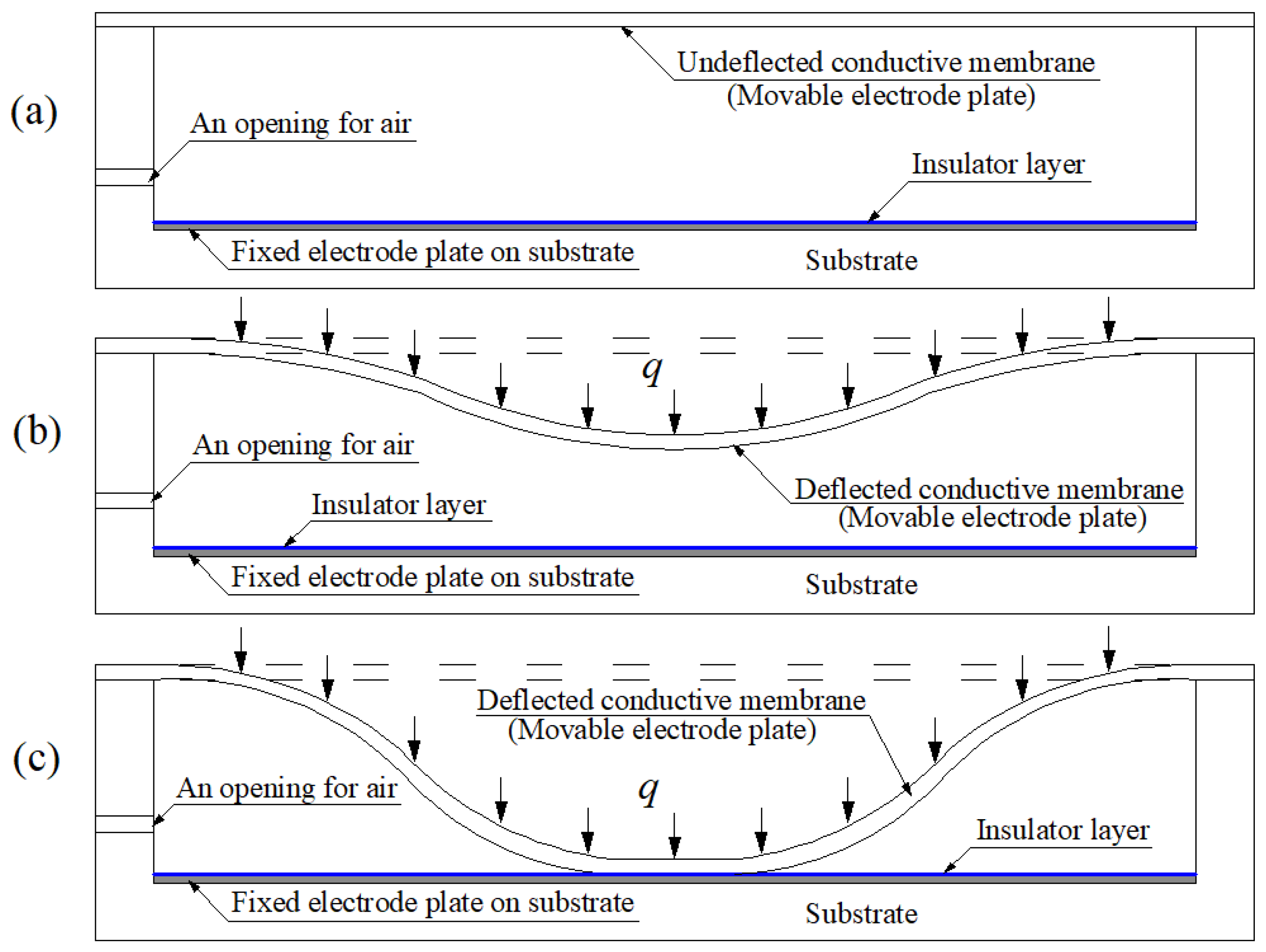
Figure 1.
Sketch of the structure and modes of operation of a membrane elastic deflection-based capacitive pressure sensor: (a) the initial status without application of the pressure q, (b) non-touch mode of operation under the pressure q, and (c) touch mode of operation under the pressure q.
Figure 1.
Sketch of the structure and modes of operation of a membrane elastic deflection-based capacitive pressure sensor: (a) the initial status without application of the pressure q, (b) non-touch mode of operation under the pressure q, and (c) touch mode of operation under the pressure q.
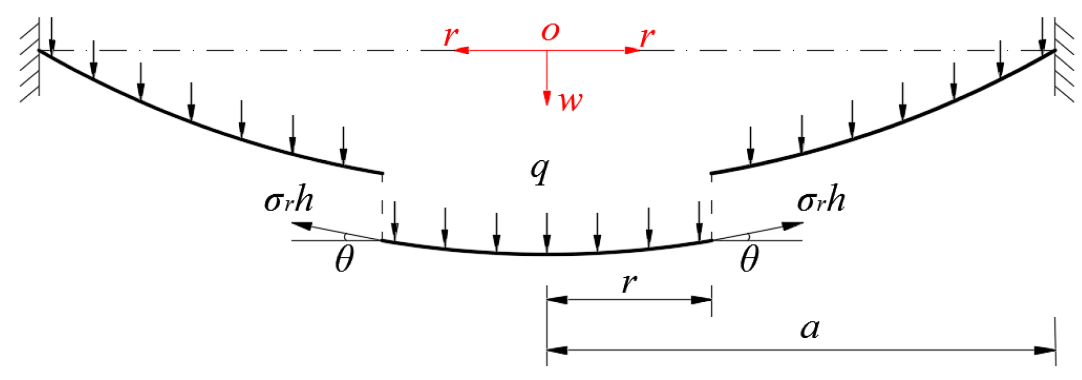
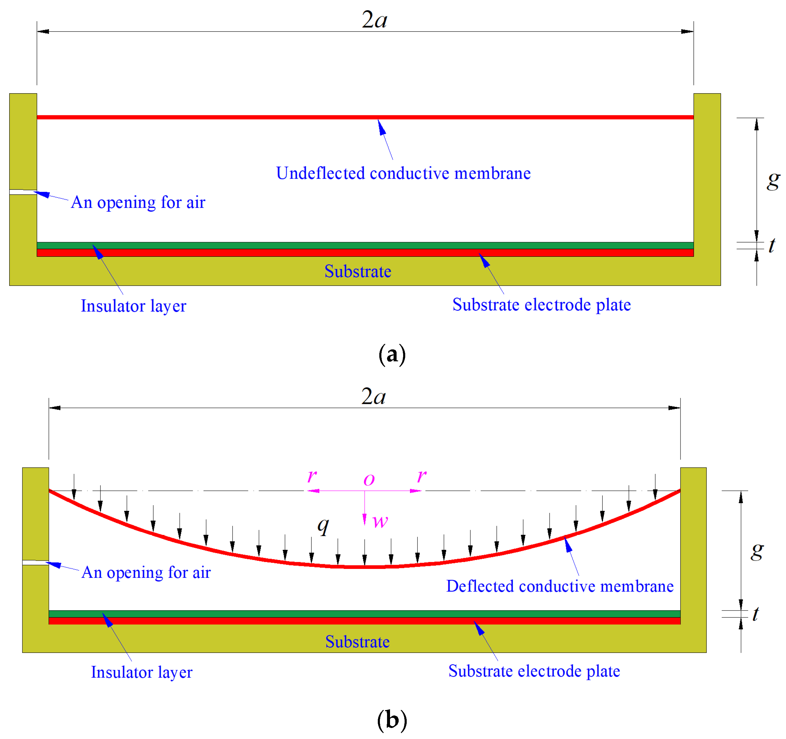
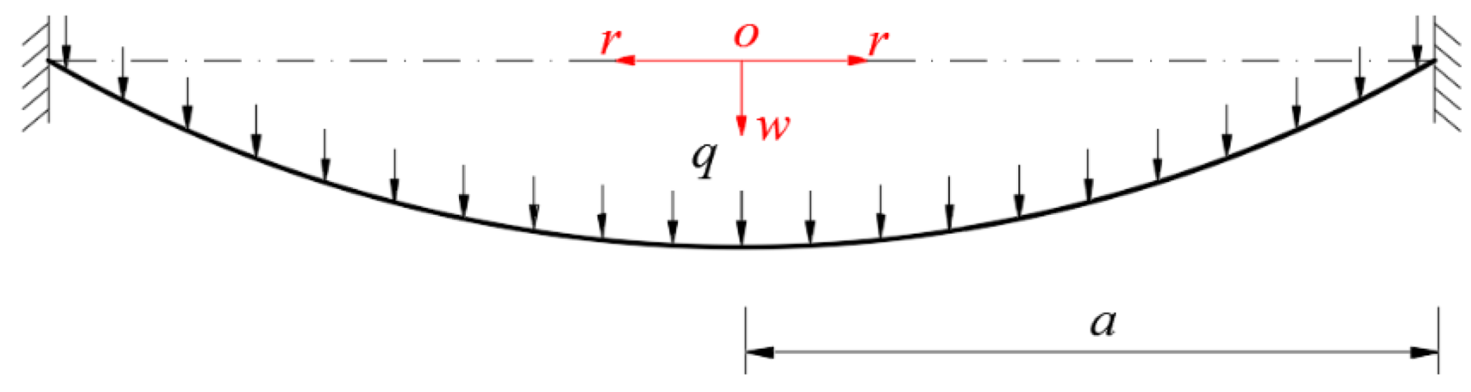
Figure 2.
Sketch of the capacitive pressure sensor: (a) initial state and (b) operating state.
Figure 2.
Sketch of the capacitive pressure sensor: (a) initial state and (b) operating state.
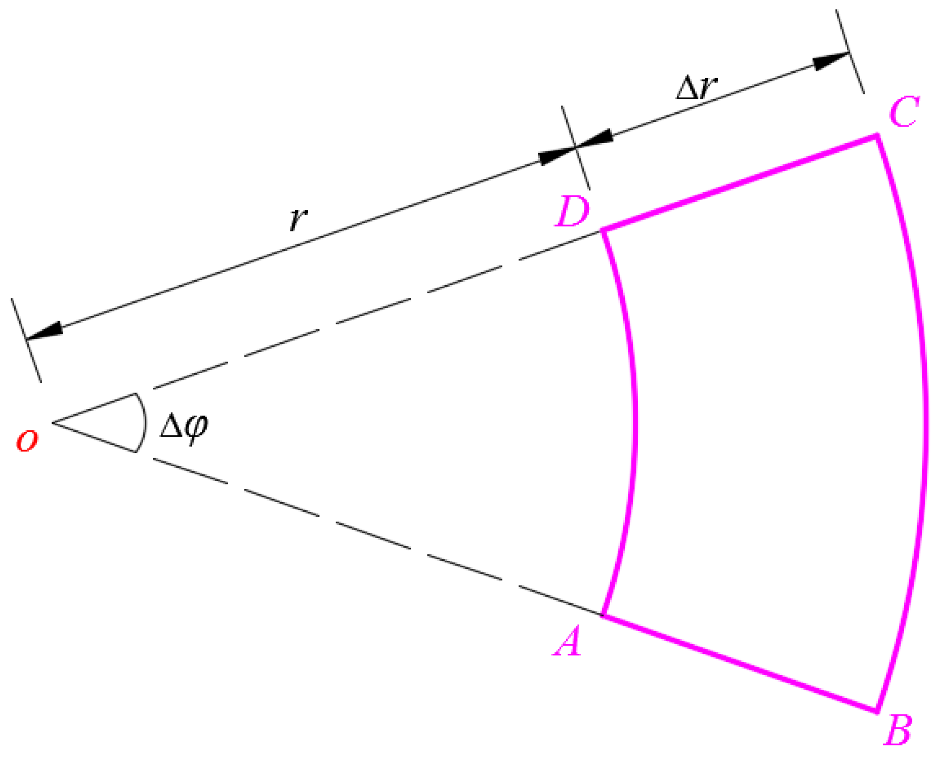
Figure 3.
Sketch of the micro area element ABCD taken from the substrate electrode plate.
Figure 3.
Sketch of the micro area element ABCD taken from the substrate electrode plate.
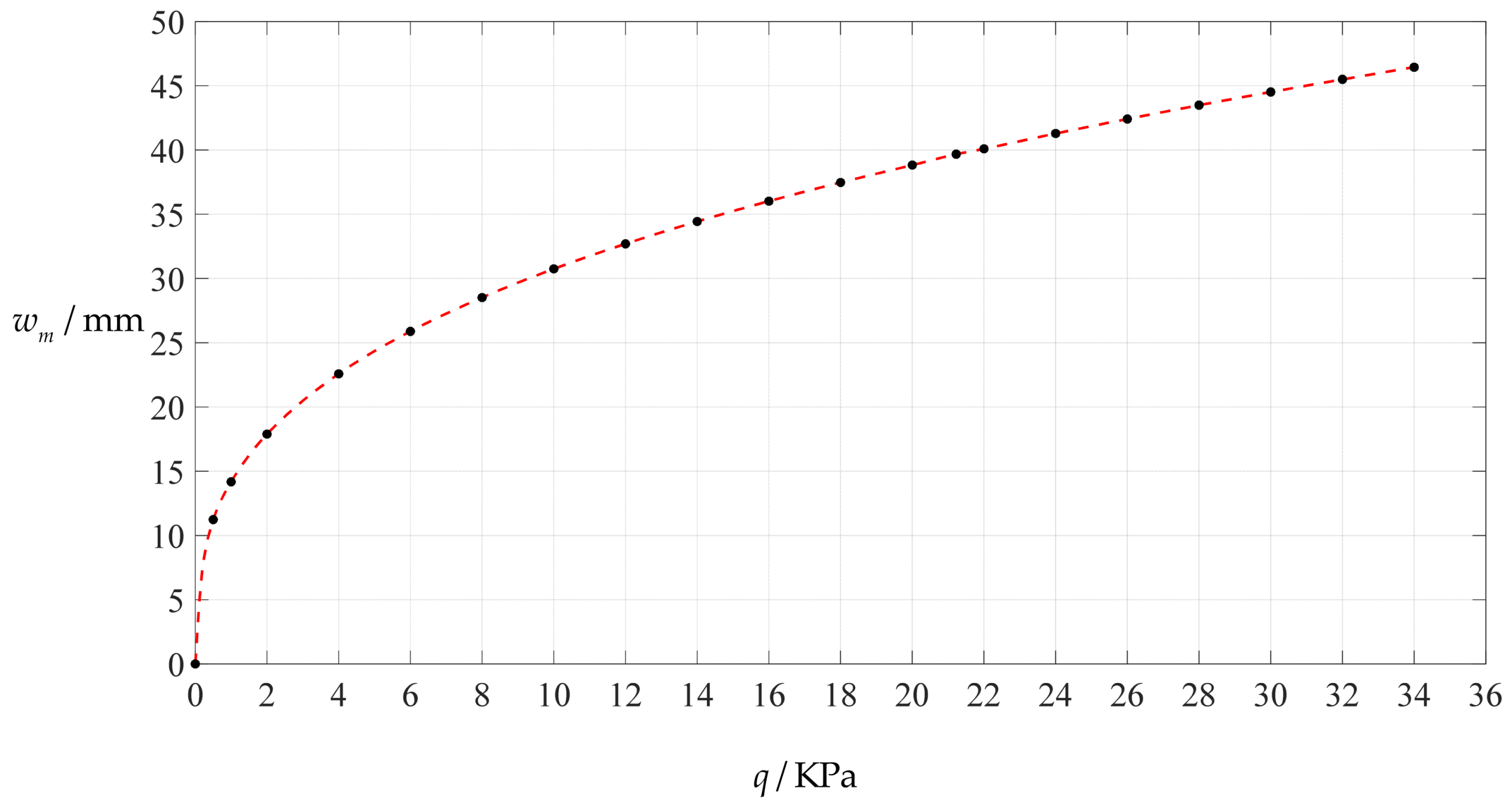
Figure 4.
Variation of maximum deflection wm with pressure q.
Figure 4.
Variation of maximum deflection wm with pressure q.
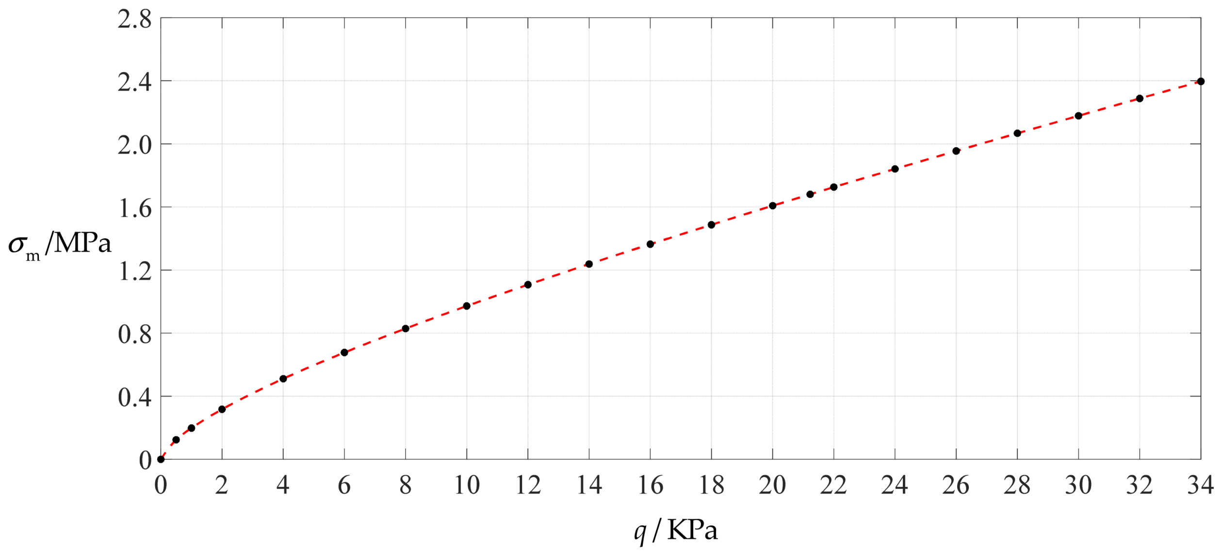
Figure 5.
Variation of maximum stress σm with pressure q.
Figure 5.
Variation of maximum stress σm with pressure q.
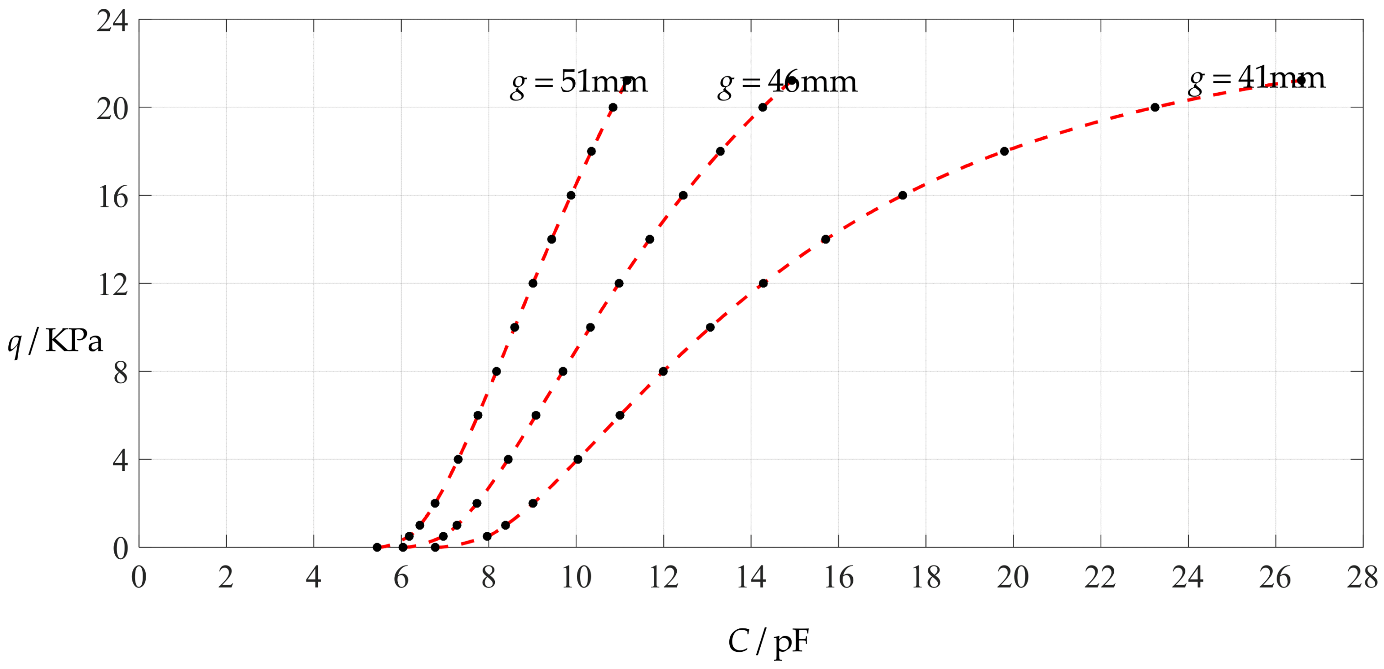
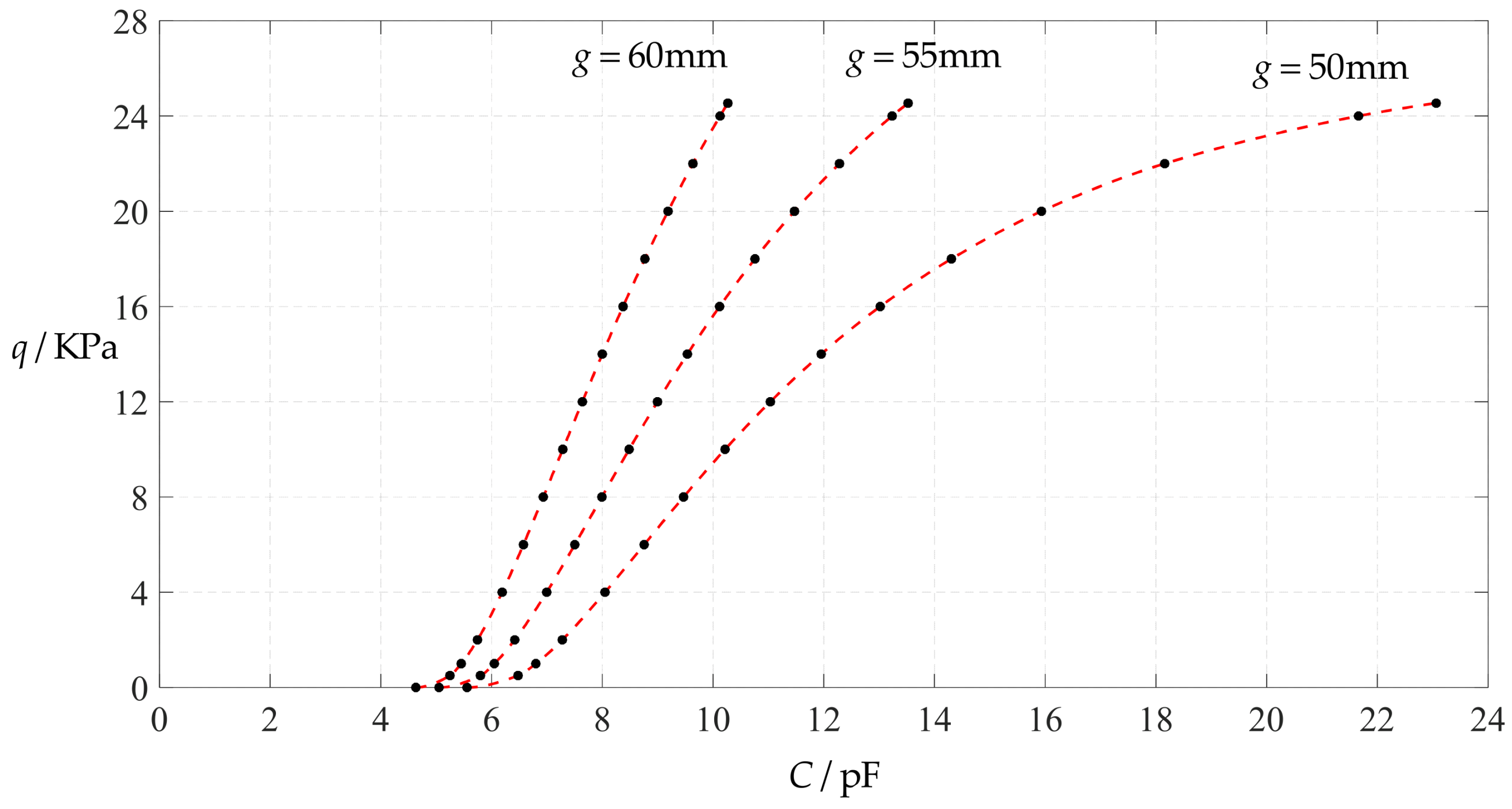
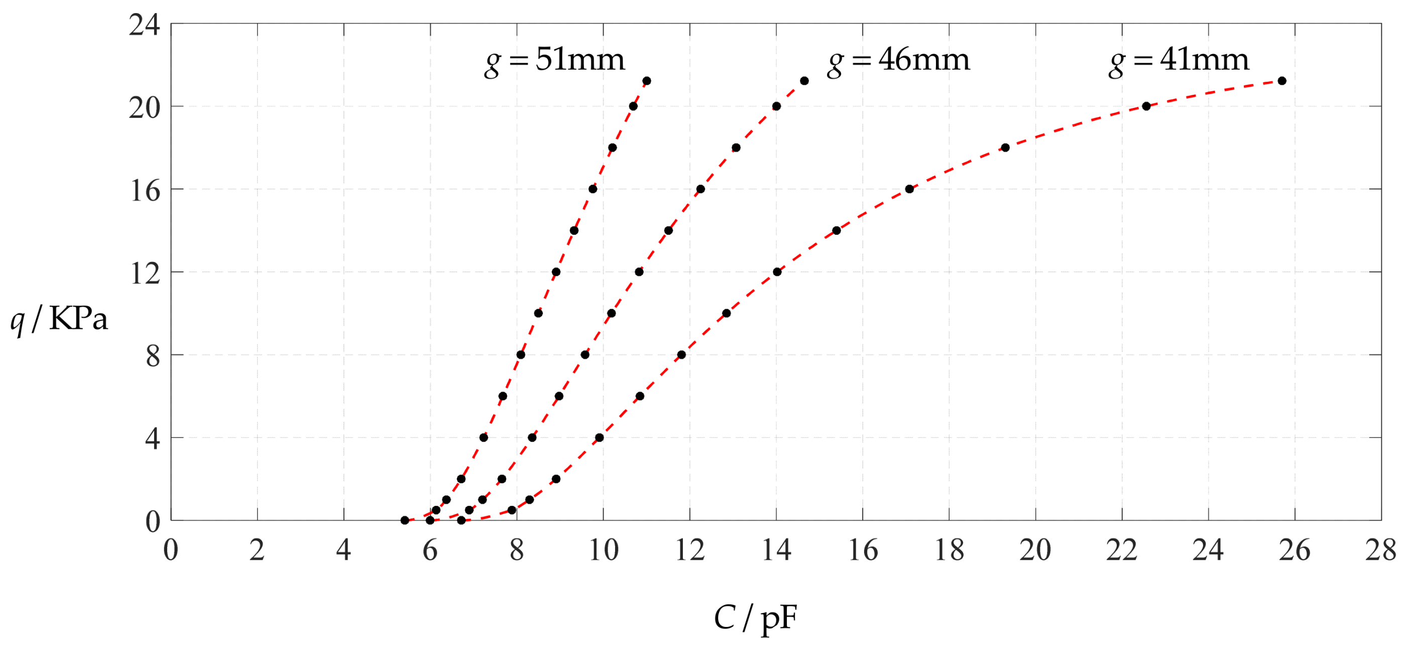
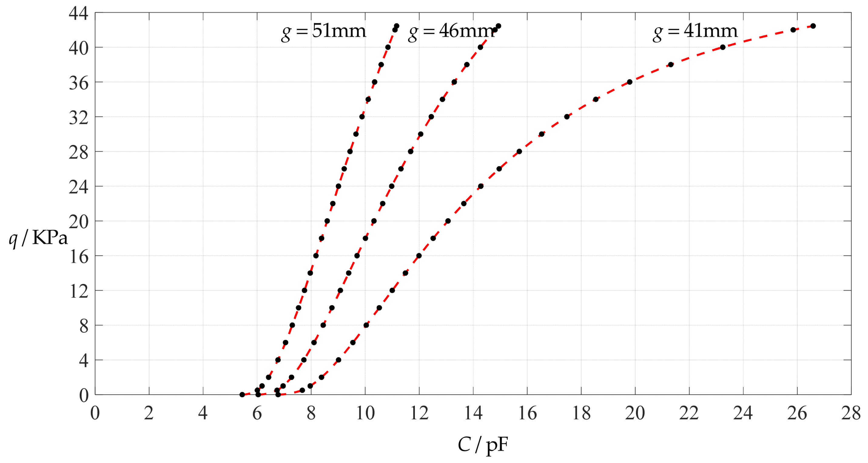
Figure 6.
Variations of pressure q with capacitance C, when a = 100 mm, h = 1 mm, E = 7.84 MPa, ν = 0.47, t = 0.1 mm, and g = 41 mm, 45 mm and 51 mm.
Figure 6.
Variations of pressure q with capacitance C, when a = 100 mm, h = 1 mm, E = 7.84 MPa, ν = 0.47, t = 0.1 mm, and g = 41 mm, 45 mm and 51 mm.
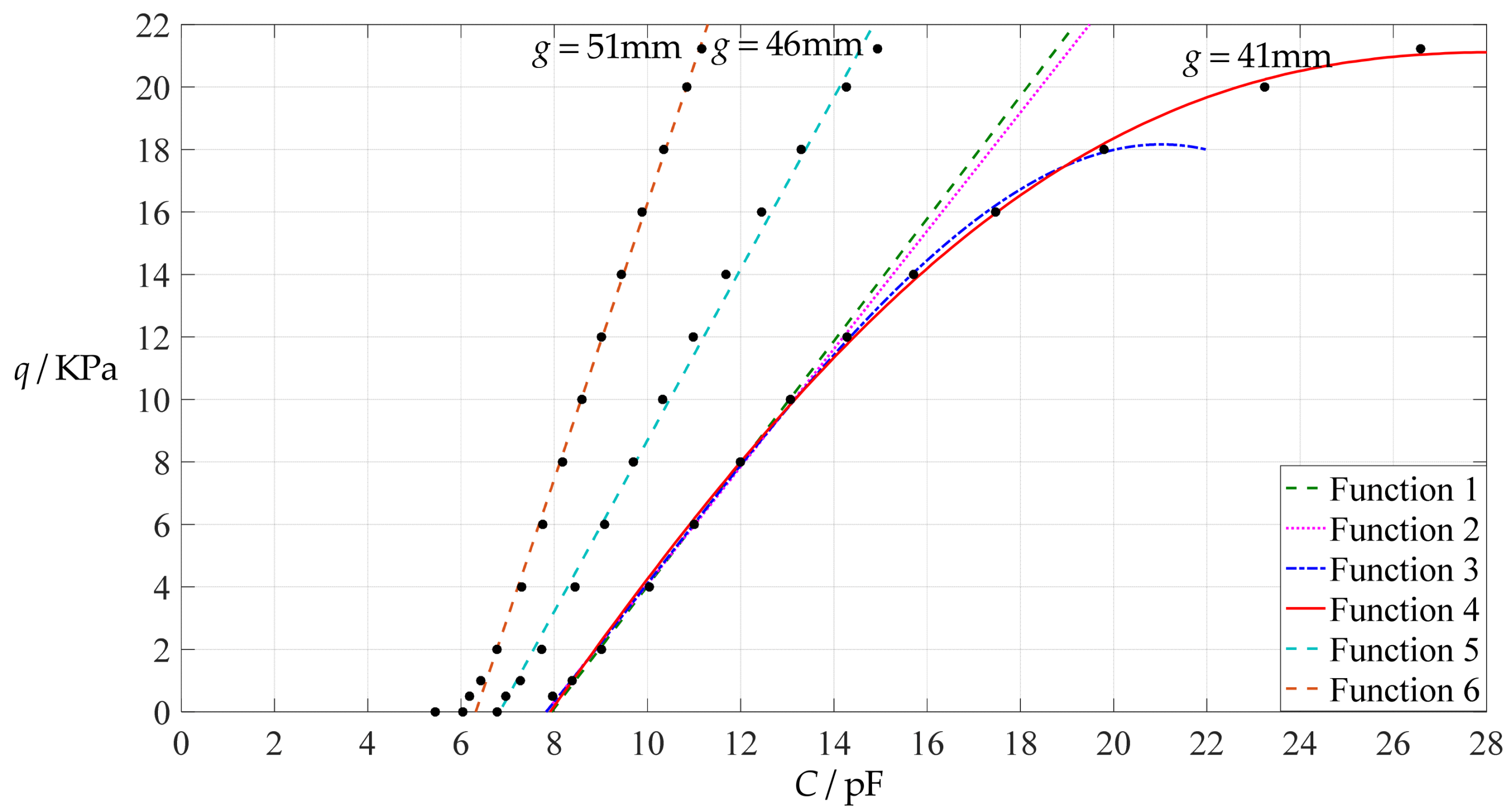
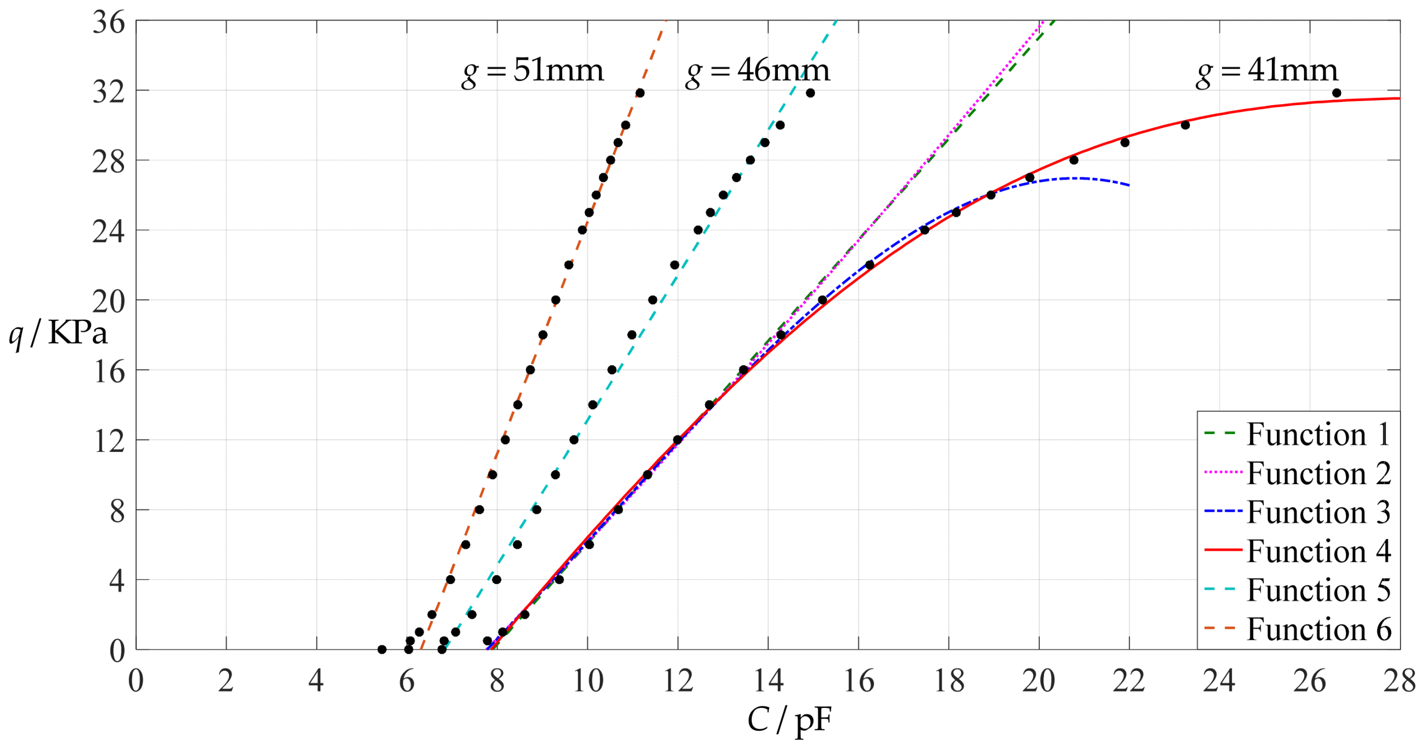
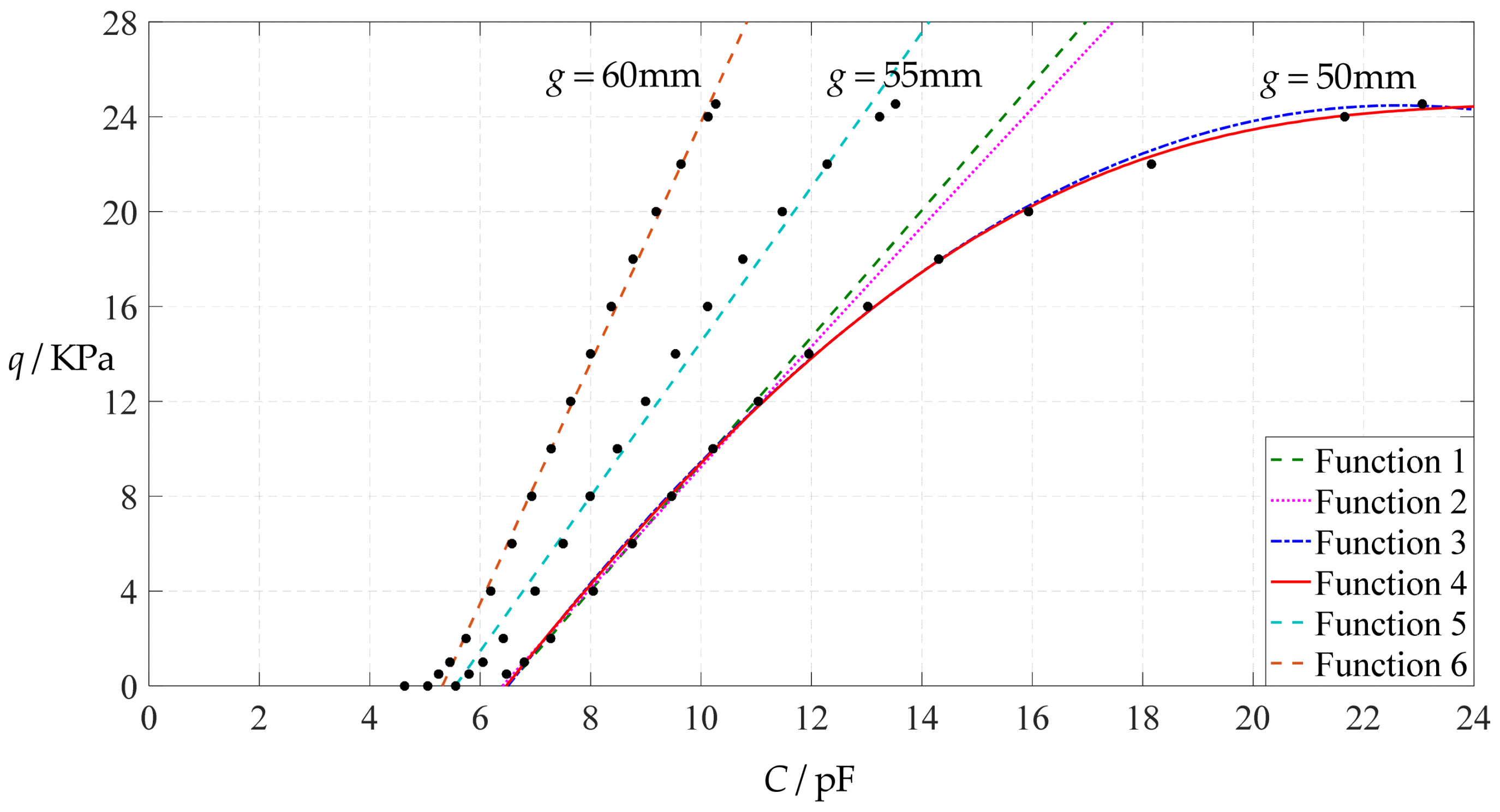
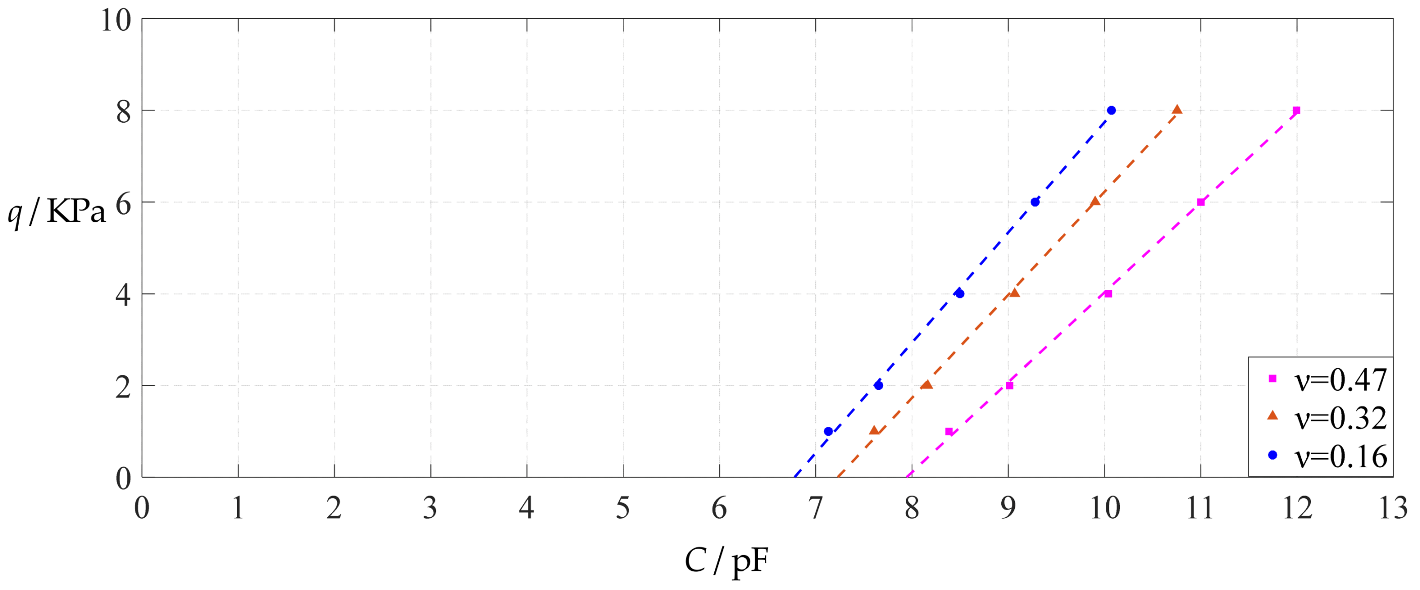
Figure 7.
Least-squares fitting of the relationships between
q and
C in
Figure 6.
Figure 7.
Least-squares fitting of the relationships between
q and
C in
Figure 6.
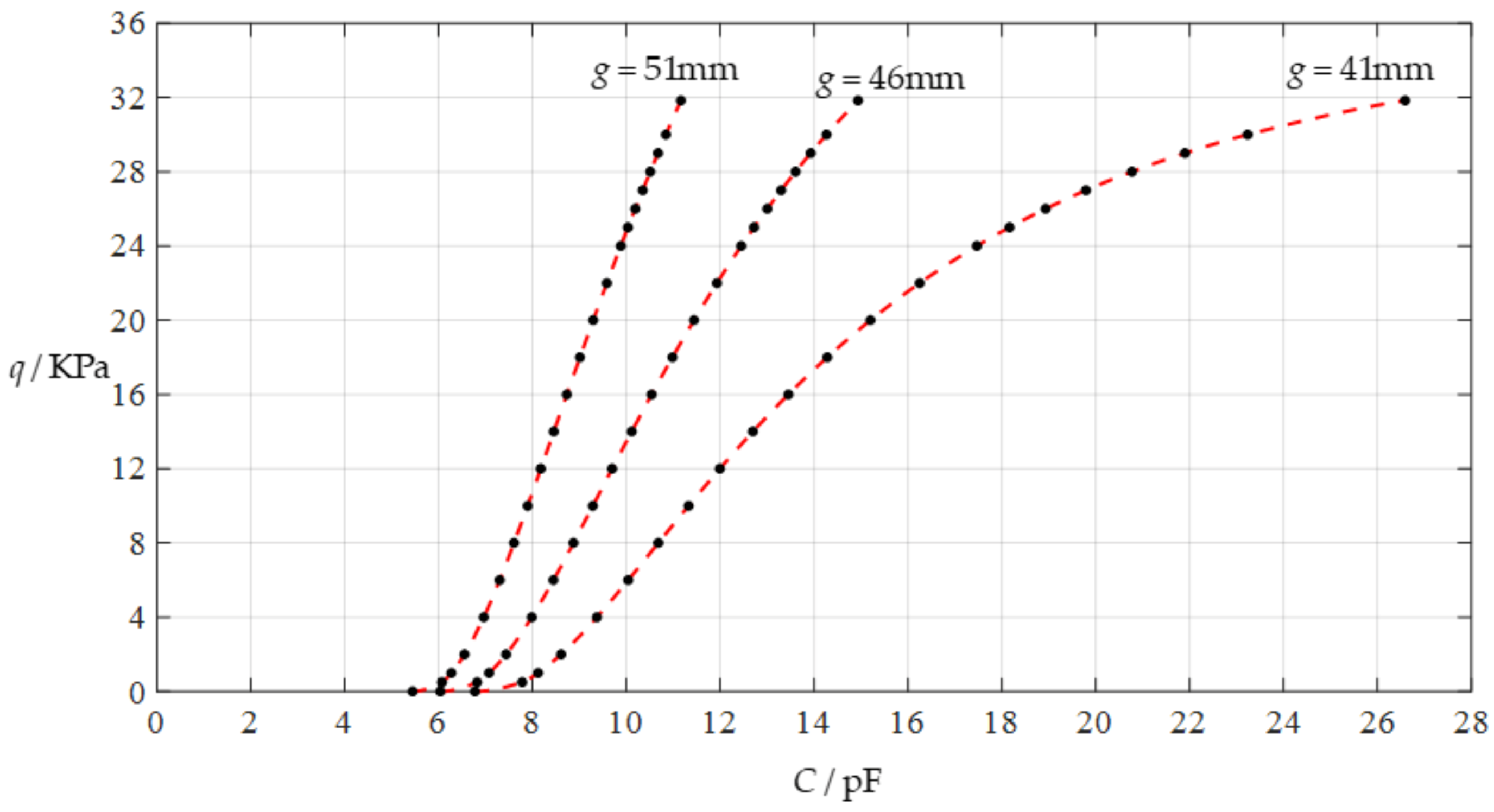
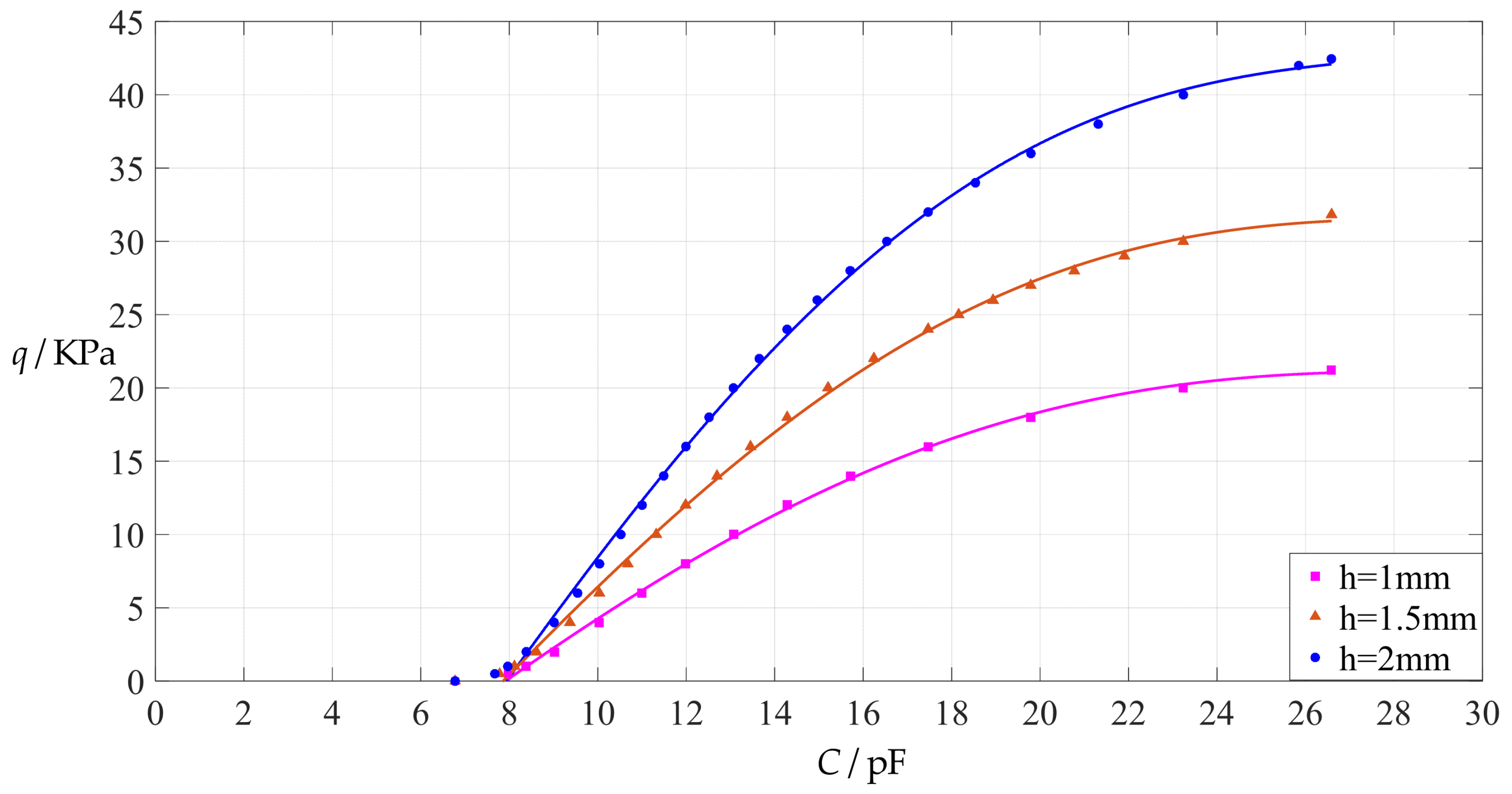
Figure 8.
Variations of pressure q with capacitance C, when a = 100 mm, h = 1.5 mm, E = 7.84 MPa, ν = 0.47, t = 0.1 mm, and g = 41 mm, 46 mm and 51 mm.
Figure 8.
Variations of pressure q with capacitance C, when a = 100 mm, h = 1.5 mm, E = 7.84 MPa, ν = 0.47, t = 0.1 mm, and g = 41 mm, 46 mm and 51 mm.
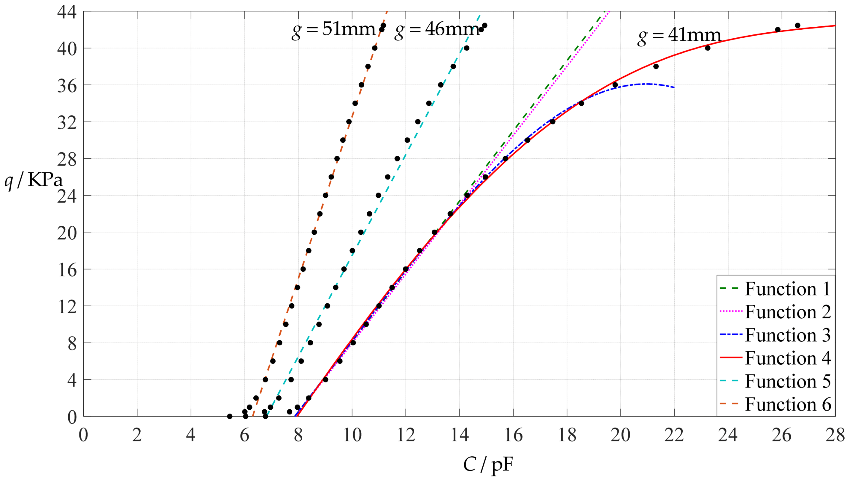
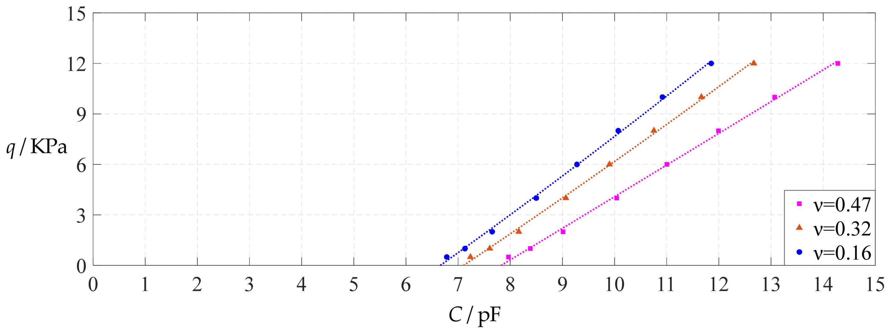
Figure 9.
Least-squares fitting of the relationships between
q and
C in
Figure 8.
Figure 9.
Least-squares fitting of the relationships between
q and
C in
Figure 8.
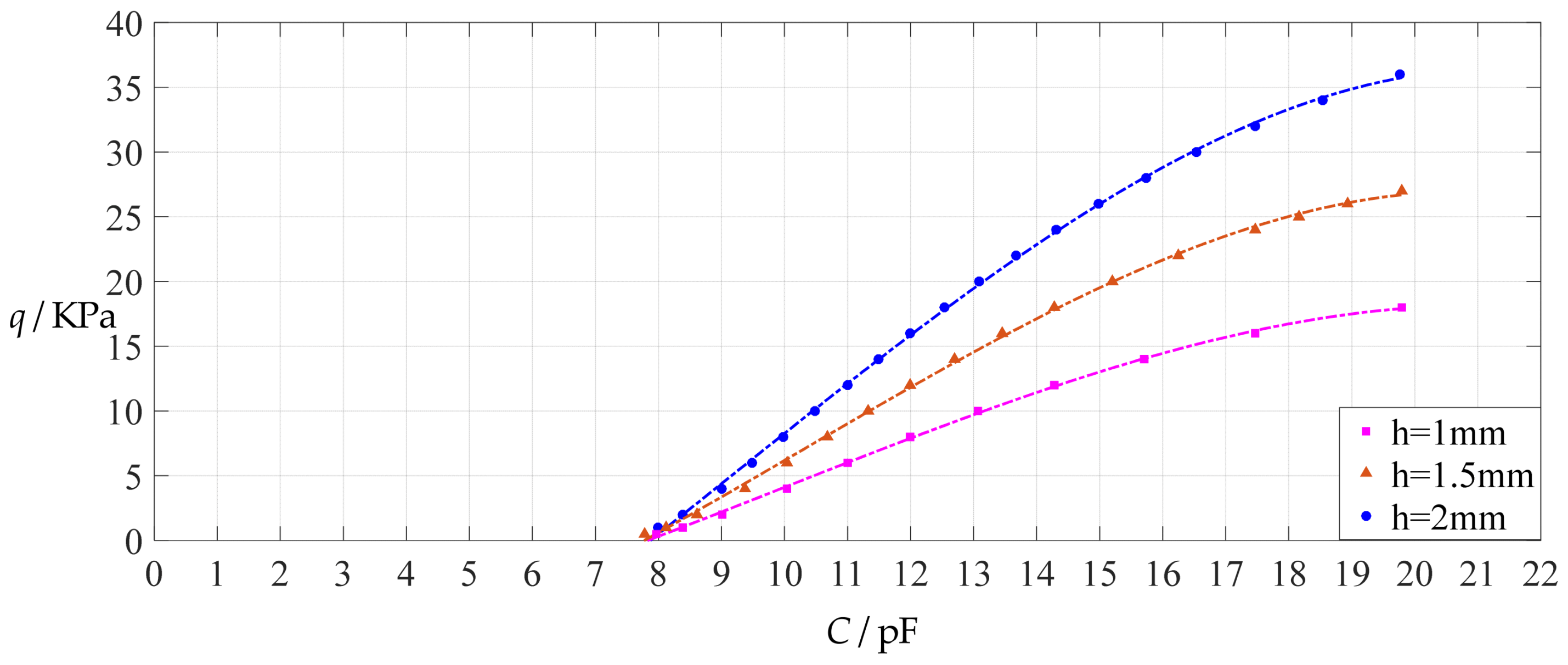
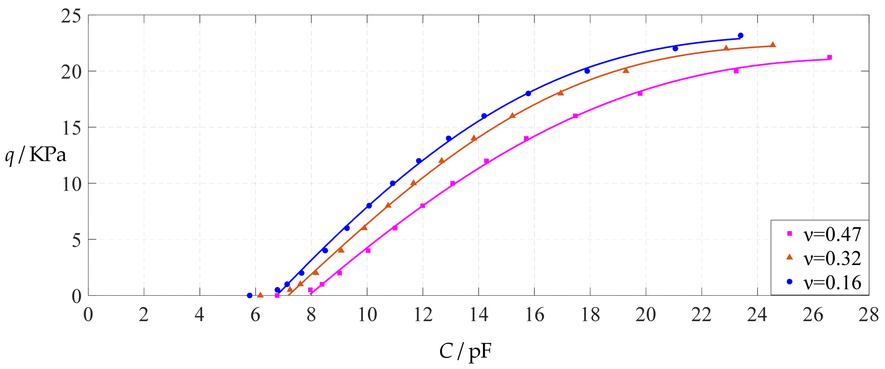
Figure 10.
Variations of pressure q with capacitance C, when a = 100 mm, h = 2 mm, E = 7.84 MPa, ν = 0.47, t = 0.1 mm, and g = 41 mm, 46 mm and 51 mm.
Figure 10.
Variations of pressure q with capacitance C, when a = 100 mm, h = 2 mm, E = 7.84 MPa, ν = 0.47, t = 0.1 mm, and g = 41 mm, 46 mm and 51 mm.
Figure 11.
Least-squares fitting of the relationships between
q and
C in
Figure 10.
Figure 11.
Least-squares fitting of the relationships between
q and
C in
Figure 10.
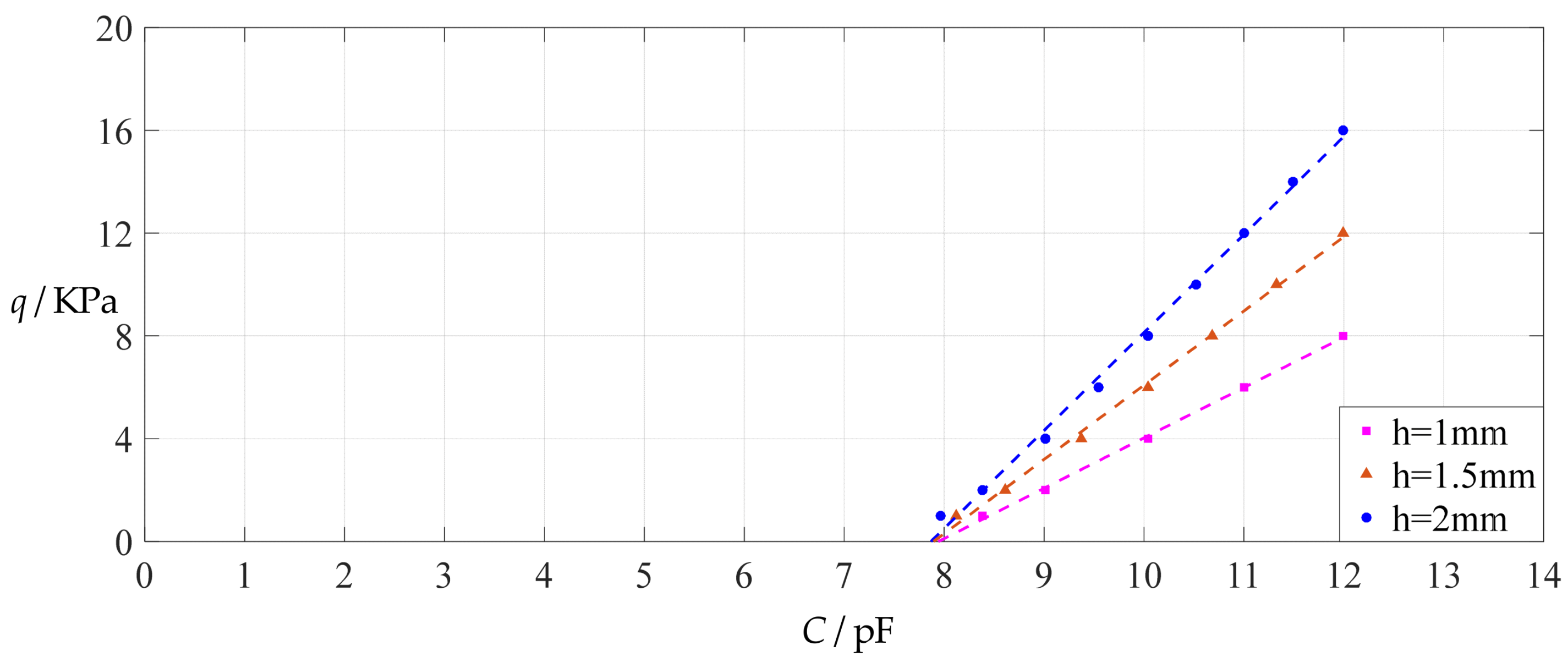
Figure 12.
The effect of changing the membrane thickness
h on Function 1 in
Table 5,
Table 7 and
Table 9 (fitted by a straight line).
Figure 12.
The effect of changing the membrane thickness
h on Function 1 in
Table 5,
Table 7 and
Table 9 (fitted by a straight line).
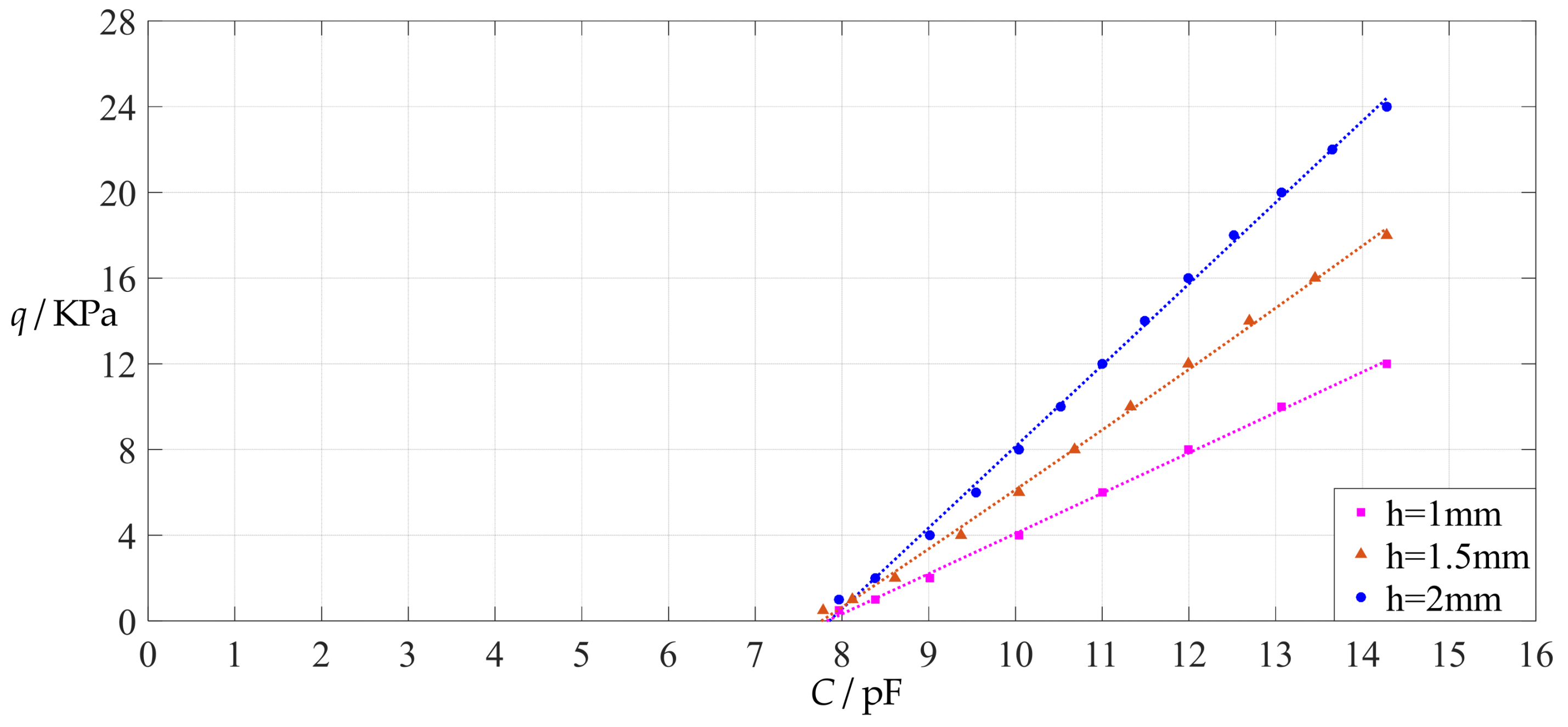
Figure 13.
The effect of changing the membrane thickness
h on Function 2 in
Table 5,
Table 7 and
Table 9 (fitted by a quadratic function).
Figure 13.
The effect of changing the membrane thickness
h on Function 2 in
Table 5,
Table 7 and
Table 9 (fitted by a quadratic function).
Figure 14.
The effect of changing the membrane thickness
h on Function 3 in
Table 5,
Table 7 and
Table 9 (fitted by a cubic function).
Figure 14.
The effect of changing the membrane thickness
h on Function 3 in
Table 5,
Table 7 and
Table 9 (fitted by a cubic function).
Figure 15.
The effect of changing the membrane thickness
h on Function 4 in
Table 5,
Table 7 and
Table 9 (fitted by a quartic function).
Figure 15.
The effect of changing the membrane thickness
h on Function 4 in
Table 5,
Table 7 and
Table 9 (fitted by a quartic function).
Figure 16.
Variations of pressure q with capacitance C, when a = 100 mm, h = 1 mm, E = 5 MPa, ν = 0.47, t = 0.1 mm and g = 41 mm, 46 mm and 51 mm.
Figure 16.
Variations of pressure q with capacitance C, when a = 100 mm, h = 1 mm, E = 5 MPa, ν = 0.47, t = 0.1 mm and g = 41 mm, 46 mm and 51 mm.
Figure 17.
Least-squares fitting of the relationships between
q and
C in
Figure 16.
Figure 17.
Least-squares fitting of the relationships between
q and
C in
Figure 16.
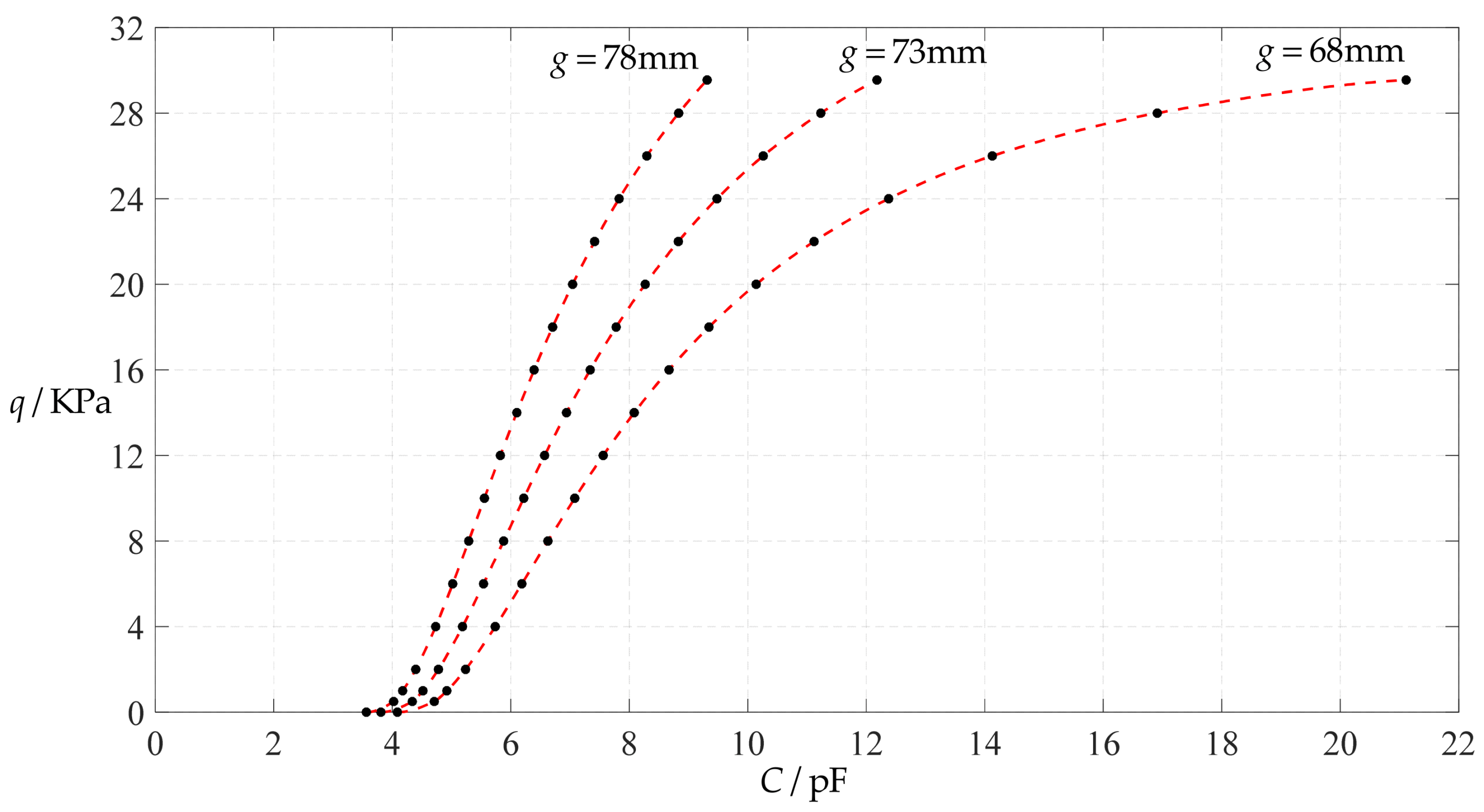
Figure 18.
Variations of pressure q with capacitance C, when a = 100 mm, h = 1 mm, E = 2.5 MPa, ν = 0.47, t = 0.1 mm, and g = 68 mm, 73 mm and 78 mm.
Figure 18.
Variations of pressure q with capacitance C, when a = 100 mm, h = 1 mm, E = 2.5 MPa, ν = 0.47, t = 0.1 mm, and g = 68 mm, 73 mm and 78 mm.
Figure 19.
Least-squares fitting of the relationships between
q and
C in
Figure 18.
Figure 19.
Least-squares fitting of the relationships between
q and
C in
Figure 18.
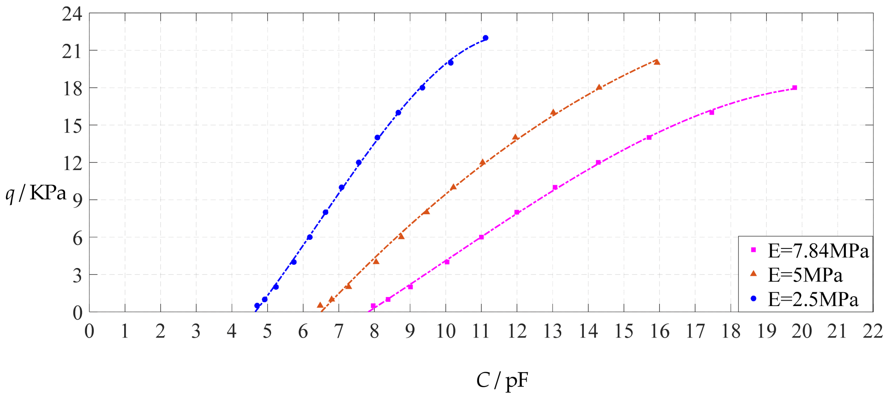
Figure 20.
The effect of changing the Young’s modulus of elasticity
E on Function 1 in
Table 5,
Table 11 and
Table 13 (fitted by a straight line).
Figure 20.
The effect of changing the Young’s modulus of elasticity
E on Function 1 in
Table 5,
Table 11 and
Table 13 (fitted by a straight line).
Figure 21.
The effect of changing the Young’s modulus of elasticity
E on Function 2 in
Table 5,
Table 11 and
Table 13 (fitted by a quadratic function).
Figure 21.
The effect of changing the Young’s modulus of elasticity
E on Function 2 in
Table 5,
Table 11 and
Table 13 (fitted by a quadratic function).
Figure 22.
The effect of changing the Young’s modulus of elasticity
E on Function 3 in
Table 5,
Table 11 and
Table 13 (fitted by a cubic function).
Figure 22.
The effect of changing the Young’s modulus of elasticity
E on Function 3 in
Table 5,
Table 11 and
Table 13 (fitted by a cubic function).
Figure 23.
The effect of changing the Young’s modulus of elasticity
E on Function 4 in
Table 5,
Table 11 and
Table 13 (fitted by a quartic function).
Figure 23.
The effect of changing the Young’s modulus of elasticity
E on Function 4 in
Table 5,
Table 11 and
Table 13 (fitted by a quartic function).
Figure 24.
Variations of pressure q with capacitance C, when a = 100 mm, h = 1 mm, E = 7.84 MPa, ν = 0.32, t = 0.1 mm and g = 45 mm, 50 mm and 55 mm.
Figure 24.
Variations of pressure q with capacitance C, when a = 100 mm, h = 1 mm, E = 7.84 MPa, ν = 0.32, t = 0.1 mm and g = 45 mm, 50 mm and 55 mm.
Figure 25.
Least-squares fitting of the relationships between
q and
C in
Figure 24.
Figure 25.
Least-squares fitting of the relationships between
q and
C in
Figure 24.
Figure 26.
Variations of pressure q with capacitance C, when a = 100 mm, h = 1 mm, E = 7.84 MPa, ν = 0.16, t = 0.1 mm and g = 48 mm, 53 mm and 58 mm.
Figure 26.
Variations of pressure q with capacitance C, when a = 100 mm, h = 1 mm, E = 7.84 MPa, ν = 0.16, t = 0.1 mm and g = 48 mm, 53 mm and 58 mm.
Figure 27.
Least-squares fitting of the relationships between
q and
C in
Figure 26.
Figure 27.
Least-squares fitting of the relationships between
q and
C in
Figure 26.
Figure 28.
The effect of changing the Poisson’s ratio
v on Function 1 in
Table 5,
Table 15 and
Table 17 (fitted by a straight line).
Figure 28.
The effect of changing the Poisson’s ratio
v on Function 1 in
Table 5,
Table 15 and
Table 17 (fitted by a straight line).
Figure 29.
The effect of changing the Poisson’s ratio
v on Function 2 in
Table 5,
Table 15 and
Table 17 (fitted by a quadratic function).
Figure 29.
The effect of changing the Poisson’s ratio
v on Function 2 in
Table 5,
Table 15 and
Table 17 (fitted by a quadratic function).
Figure 30.
The effect of changing the Poisson’s ratio
v on Function 3 in
Table 5,
Table 15 and
Table 17 (fitted by a cubic function).
Figure 30.
The effect of changing the Poisson’s ratio
v on Function 3 in
Table 5,
Table 15 and
Table 17 (fitted by a cubic function).
Figure 31.
The effect of changing the Poisson’s ratio
v on Function 4 in
Table 5,
Table 15 and
Table 17 (fitted by a quartic function).
Figure 31.
The effect of changing the Poisson’s ratio
v on Function 4 in
Table 5,
Table 15 and
Table 17 (fitted by a quartic function).
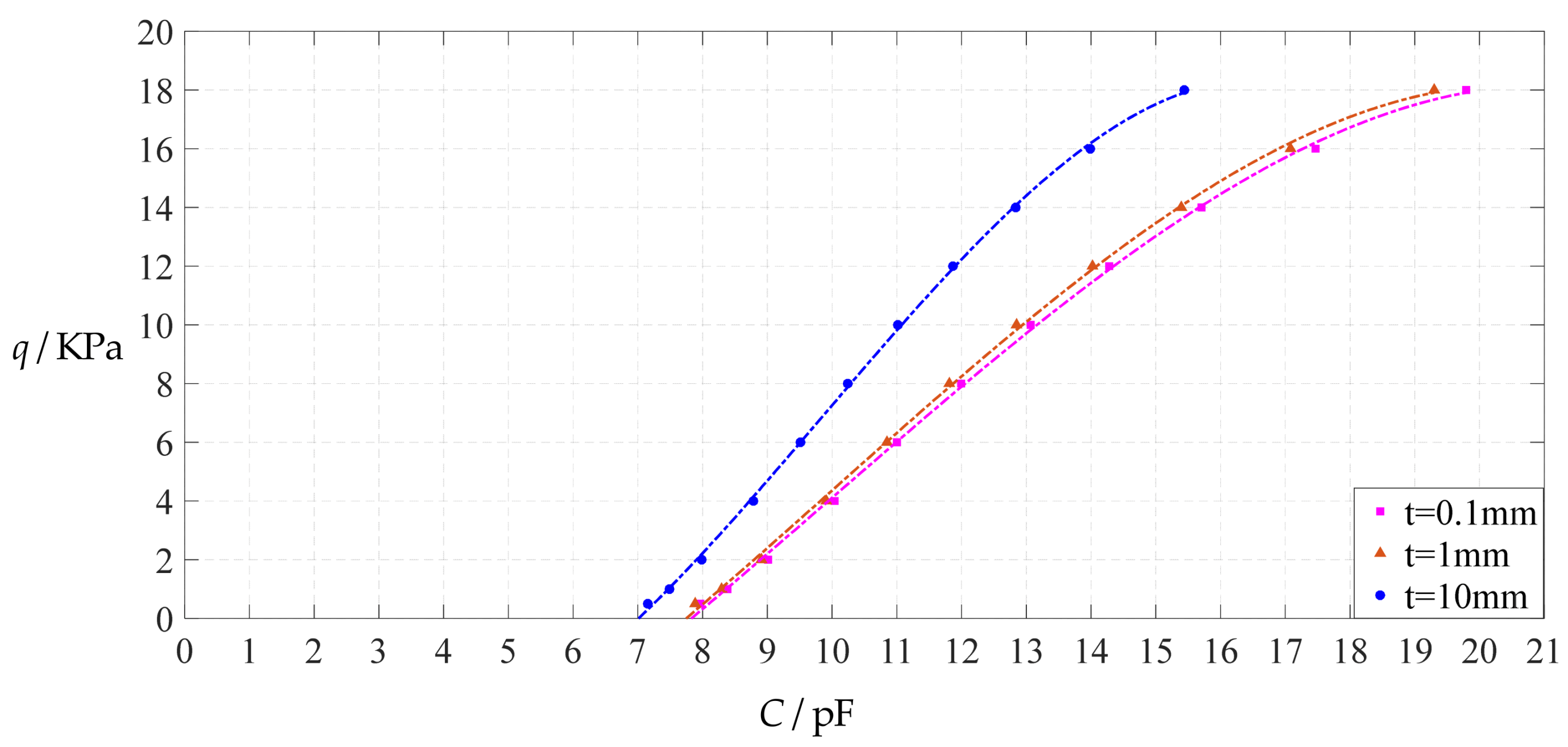
Figure 32.
Variations of pressure q with capacitance C, when a = 100 mm, h = 1 mm, E = 7.84 MPa, ν = 0.47, t = 1 mm and g = 41 mm, 46 mm and 51 mm.
Figure 32.
Variations of pressure q with capacitance C, when a = 100 mm, h = 1 mm, E = 7.84 MPa, ν = 0.47, t = 1 mm and g = 41 mm, 46 mm and 51 mm.
Figure 33.
Least-squares fitting of the relationships between
q and
C in
Figure 32.
Figure 33.
Least-squares fitting of the relationships between
q and
C in
Figure 32.
Figure 34.
Variations of pressure q with capacitance C, when a = 100 mm, h = 1 mm, E = 7.84 MPa, ν = 0.47, t = 10 mm and g = 41 mm, 46 mm and 51 mm.
Figure 34.
Variations of pressure q with capacitance C, when a = 100 mm, h = 1 mm, E = 7.84 MPa, ν = 0.47, t = 10 mm and g = 41 mm, 46 mm and 51 mm.
Figure 35.
Least-squares fitting of the relationships between
q and
C in
Figure 34.
Figure 35.
Least-squares fitting of the relationships between
q and
C in
Figure 34.
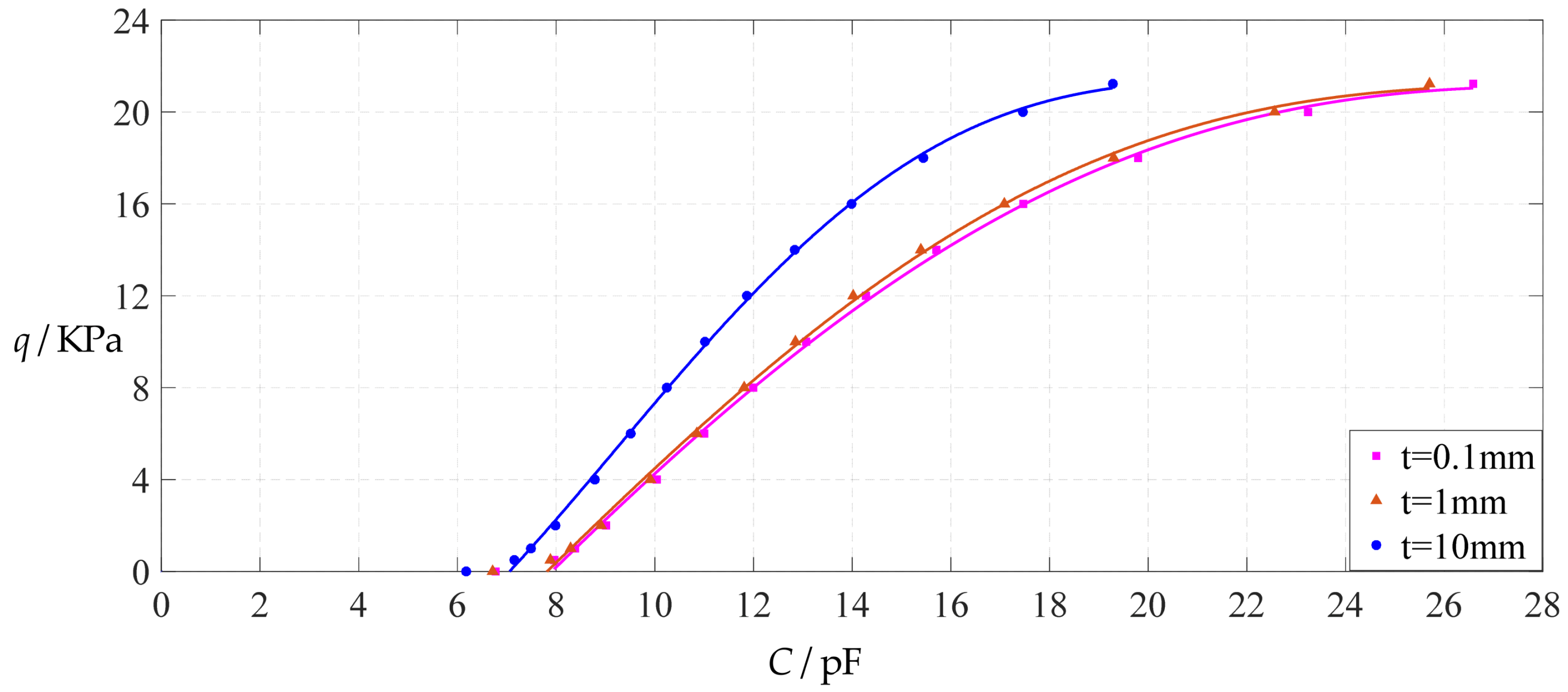
Figure 36.
The effect of changing the insulator layer thickness
t on Function 1 in
Table 5,
Table 19 and
Table 21 (fitted by a straight line).
Figure 36.
The effect of changing the insulator layer thickness
t on Function 1 in
Table 5,
Table 19 and
Table 21 (fitted by a straight line).
Figure 37.
The effect of changing the insulator layer thickness
t on Function 2 in
Table 5,
Table 19 and
Table 21 (fitted by a quadratic function).
Figure 37.
The effect of changing the insulator layer thickness
t on Function 2 in
Table 5,
Table 19 and
Table 21 (fitted by a quadratic function).
Figure 38.
The effect of changing the insulator layer thickness
t on Function 3 in
Table 5,
Table 19 and
Table 21 (fitted by a cubic function).
Figure 38.
The effect of changing the insulator layer thickness
t on Function 3 in
Table 5,
Table 19 and
Table 21 (fitted by a cubic function).
Figure 39.
The effect of changing the insulator layer thickness
t on Function 4 in
Table 5,
Table 19 and
Table 21 (fitted by a quartic function).
Figure 39.
The effect of changing the insulator layer thickness
t on Function 4 in
Table 5,
Table 19 and
Table 21 (fitted by a quartic function).
Table 1.
The calculation results of b0 and c0, wm and σm for a = 100 mm, h = 1 mm, E = 7.84 MPa and ν = 0.47.
Table 1.
The calculation results of b0 and c0, wm and σm for a = 100 mm, h = 1 mm, E = 7.84 MPa and ν = 0.47.
| q/KPa | b0 | c0 | wm/mm | σm/MPa |
|---|
| 0 | 0.000000 | 0.000000 | 0.000 | 0.000 |
| 0.5 | 0.015819 | 0.112374 | 11.237 | 0.124 |
| 1 | 0.025251 | 0.141729 | 14.173 | 0.198 |
| 2 | 0.040443 | 0.178839 | 17.884 | 0.317 |
| 4 | 0.065119 | 0.225793 | 22.579 | 0.511 |
| 6 | 0.086362 | 0.258841 | 25.884 | 0.677 |
| 8 | 0.105751 | 0.285194 | 28.519 | 0.829 |
| 10 | 0.123933 | 0.307465 | 30.747 | 0.972 |
| 12 | 0.141247 | 0.326937 | 32.694 | 1.107 |
| 14 | 0.157901 | 0.344351 | 34.435 | 1.238 |
| 16 | 0.174030 | 0.360175 | 36.018 | 1.364 |
| 18 | 0.189729 | 0.374732 | 37.473 | 1.487 |
| 20 | 0.205068 | 0.388252 | 38.825 | 1.608 |
| 21.225 | 0.214308 | 0.396696 | 39.670 | 1.680 |
| 22 | 0.220099 | 0.400906 | 40.091 | 1.726 |
| 24 | 0.234862 | 0.412826 | 41.283 | 1.841 |
| 26 | 0.249389 | 0.424116 | 42.412 | 1.955 |
| 28 | 0.263707 | 0.434859 | 43.486 | 2.067 |
| 30 | 0.277838 | 0.445123 | 44.512 | 2.178 |
| 32 | 0.291798 | 0.454965 | 45.496 | 2.288 |
| 34 | 0.305603 | 0.464432 | 46.443 | 2.396 |
Table 2.
The calculation results of the coefficients c2i (i = 0, 1, 2, 3) for a = 100 mm, h = 1 mm, E = 7.84 MPa and ν = 0.47.
Table 2.
The calculation results of the coefficients c2i (i = 0, 1, 2, 3) for a = 100 mm, h = 1 mm, E = 7.84 MPa and ν = 0.47.
| q/KPa | c0 | c2 | c4 | c6 |
|---|
| 0 | 0.000000 | 0.000000 | 0.000000 | 0.000000 |
| 0.5 | 0.112374 | −0.100790 | −0.009047 | −1.854564 × 10⁻³ |
| 1 | 0.141729 | −0.126281 | −0.011851 | −2.564440 × 10⁻³ |
| 2 | 0.178839 | −0.157694 | −0.015787 | −3.678232 × 10⁻³ |
| 4 | 0.225793 | −0.195873 | −0.021459 | −5.497780 × 10⁻³ |
| 6 | 0.258841 | −0.221541 | −0.025922 | −7.084793 × 10⁻³ |
| 8 | 0.285194 | −0.241228 | −0.029749 | −8.541169 × 10⁻³ |
| 10 | 0.307465 | −0.257299 | −0.033155 | −9.905430 × 10⁻³ |
| 12 | 0.326937 | −0.270910 | −0.036253 | −1.119777 × 10⁻² |
| 14 | 0.344351 | −0.282727 | −0.039109 | −1.243081 × 10⁻² |
| 16 | 0.360175 | −0.293170 | −0.041768 | −1.361335 × 10⁻² |
| 18 | 0.374732 | −0.302525 | −0.044262 | −1.475200 × 10⁻² |
| 20 | 0.388252 | −0.310997 | −0.046617 | −1.585194 × 10⁻² |
| 21.225 | 0.396696 | −0.315815 | −0.047998 | −1.650838 × 10⁻² |
Table 3.
The calculation results of the coefficients c2i (i = 4, 5, 6, 7) for a = 100 mm, h = 1 mm, E = 7.84 MPa and ν = 0.47.
Table 3.
The calculation results of the coefficients c2i (i = 4, 5, 6, 7) for a = 100 mm, h = 1 mm, E = 7.84 MPa and ν = 0.47.
| q/KPa | c8 | c10 | c12 | c14 |
|---|
| 0 | 0.000000 | 0.000000 | 0.000000 | 0.000000 |
| 0.5 | −4.789369 × 10⁻⁴ | −1.389200 × 10⁻⁴ | −4.326591 × 10⁻⁵ | −1.414301 × 10⁻⁵ |
| 1 | −7.036597 × 10⁻⁴ | −2.176087 × 10⁻⁴ | −7.241011 × 10⁻⁵ | −2.532468 × 10⁻⁵ |
| 2 | −1.094379 × 10⁻³ | −3.682477 × 10⁻⁴ | −1.335929 × 10⁻⁴ | −5.100339 × 10⁻⁵ |
| 4 | −1.810971 × 10⁻³ | −6.767557 × 10⁻⁴ | −2.731357 × 10⁻⁴ | −1.161416 × 10⁻⁴ |
| 6 | −2.497975 × 10⁻³ | −1.000748 × 10⁻³ | −4.333885 × 10⁻⁴ | −1.978624 × 10⁻⁴ |
| 8 | −3.169617 × 10⁻³ | −1.337792 × 10⁻³ | −6.107136 × 10⁻⁴ | −2.940391 × 10⁻⁴ |
| 10 | −3.829440 × 10⁻³ | −1.684867 × 10⁻³ | −8.021195 × 10⁻⁴ | −4.028732 × 10⁻⁴ |
| 12 | −4.478700 × 10⁻³ | −2.039522 × 10⁻³ | −1.005254 × 10⁻³ | −5.228583 × 10⁻⁴ |
| 14 | −5.118047 × 10⁻³ | −2.399892 × 10⁻³ | −1.218271 × 10⁻³ | −6.527353 × 10⁻⁴ |
| 16 | −5.747980 × 10⁻³ | −2.764584 × 10⁻³ | −1.439715 × 10⁻³ | −7.914557 × 10⁻⁴ |
| 18 | −6.368975 × 10⁻³ | −3.132569 × 10⁻³ | −1.668442 × 10⁻³ | −9.381483 × 10⁻⁴ |
| 20 | −6.981522 × 10⁻³ | −3.503093 × 10⁻³ | −1.903546 × 10⁻³ | −1.092091 × 10⁻³ |
| 21.225 | −7.352749 × 10⁻³ | −3.731051 × 10⁻³ | −2.050382 × 10⁻³ | −1.189700 × 10⁻³ |
Table 4.
The calculation results for a = 100 mm, h = 1 mm, E = 7.84 MPa, ν = 0.47, t = 0.1 mm, and g = 41 mm, 46 mm and 51 mm.
Table 4.
The calculation results for a = 100 mm, h = 1 mm, E = 7.84 MPa, ν = 0.47, t = 0.1 mm, and g = 41 mm, 46 mm and 51 mm.
| q/KPa | wm/mm | σm/MPa | C/pF |
|---|
| g = 41 mm | g = 46 mm | g = 51 mm |
|---|
| 0 | 0 | 0 | 6.775 | 6.039 | 5.447 |
| 0.5 | 11.237 | 0.124 | 7.965 | 6.961 | 6.182 |
| 1 | 14.173 | 0.198 | 8.384 | 7.273 | 6.424 |
| 2 | 17.884 | 0.317 | 9.013 | 7.730 | 6.772 |
| 4 | 22.579 | 0.511 | 10.040 | 8.446 | 7.301 |
| 6 | 25.884 | 0.677 | 11.002 | 9.081 | 7.753 |
| 8 | 28.519 | 0.829 | 11.993 | 9.698 | 8.178 |
| 10 | 30.747 | 0.972 | 13.068 | 10.326 | 8.594 |
| 12 | 32.694 | 1.107 | 14.281 | 10.982 | 9.012 |
| 14 | 34.435 | 1.238 | 15.707 | 11.683 | 9.439 |
| 16 | 36.018 | 1.364 | 17.468 | 12.448 | 9.883 |
| 18 | 37.473 | 1.487 | 19.794 | 13.298 | 10.349 |
| 20 | 38.825 | 1.608 | 23.239 | 14.266 | 10.843 |
| 21.225 | 39.670 | 1.680 | 26.585 | 14.935 | 11.164 |
Table 5.
The range of pressure
q and capacitance
C, and the analytical expressions of Functions 1–6 in
Figure 7.
Table 5.
The range of pressure
q and capacitance
C, and the analytical expressions of Functions 1–6 in
Figure 7.
| Functions | q/KPa | C/pF | Functional Expressions |
|---|
| Function 1 | 1~8 | 8.384~11.993 | q = −15.57 + 1.960C |
| Function 2 | 0.5~12 | 7.965~14.281 | q = −14.59 + 1.856C − 0.001137C2 |
| Function 3 | 0.5~18 | 7.965~19.794 | q = −9.867 + 0.3584C + 0.1562C2 − 0.005222C3 |
| Function 4 | 0~21.225 | 6.775~26.585 | q = −16.64 + 1.865C + 0.06435C2 − 0.004878C3 + 0.00006859C4 |
| Function 5 | 1~21.225 | 7.273~14.935 | q = −18.73 + 2.743C |
| Function 6 | 1~21.225 | 6.424~11.164 | q = −27.93 + 4.421C |
Table 6.
The calculation results for a = 100 mm, h = 1.5 mm, E = 7.84 MPa, ν = 0.47, t = 0.1 mm, and g = 41 mm, 46 mm and 51 mm.
Table 6.
The calculation results for a = 100 mm, h = 1.5 mm, E = 7.84 MPa, ν = 0.47, t = 0.1 mm, and g = 41 mm, 46 mm and 51 mm.
| q/KPa | wm/mm | σm/MPa | C/pF |
|---|
| g = 41 mm | g = 46 mm | g = 51 mm |
|---|
| 0 | 0.000 | 0.000 | 6.775 | 6.039 | 5.447 |
| 0.5 | 9.812 | 0.094 | 7.782 | 6.822 | 6.074 |
| 1 | 12.373 | 0.151 | 8.120 | 7.077 | 6.273 |
| 2 | 15.608 | 0.241 | 8.612 | 7.440 | 6.553 |
| 4 | 19.699 | 0.386 | 9.373 | 7.986 | 6.963 |
| 6 | 22.579 | 0.511 | 10.040 | 8.446 | 7.301 |
| 8 | 24.877 | 0.624 | 10.682 | 8.874 | 7.607 |
| 10 | 26.820 | 0.729 | 11.327 | 9.287 | 7.897 |
| 12 | 28.519 | 0.829 | 11.993 | 9.698 | 8.178 |
| 14 | 30.040 | 0.925 | 12.697 | 10.114 | 8.455 |
| 16 | 31.422 | 1.018 | 13.453 | 10.540 | 8.732 |
| 18 | 32.694 | 1.107 | 14.281 | 10.982 | 9.012 |
| 20 | 33.874 | 1.195 | 15.202 | 11.443 | 9.295 |
| 22 | 34.978 | 1.281 | 16.249 | 11.930 | 9.585 |
| 24 | 36.018 | 1.364 | 17.468 | 12.448 | 9.883 |
| 25 | 36.516 | 1.406 | 18.164 | 12.720 | 10.035 |
| 26 | 37.001 | 1.447 | 18.933 | 13.004 | 10.191 |
| 27 | 37.373 | 1.487 | 19.794 | 13.298 | 10.349 |
| 28 | 37.934 | 1.528 | 20.772 | 13.606 | 10.510 |
| 29 | 38.185 | 1.568 | 21.902 | 13.928 | 10.675 |
| 30 | 38.825 | 1.608 | 23.239 | 14.266 | 10.843 |
| 31.84 | 39.611 | 1.680 | 26.591 | 14.936 | 11.164 |
Table 7.
The range of pressure
q and capacitance
C, and the analytical expressions of the Functions 1–6 in
Figure 9.
Table 7.
The range of pressure
q and capacitance
C, and the analytical expressions of the Functions 1–6 in
Figure 9.
| Functions | q/KPa | C/pF | Functional Expressions |
|---|
| Function 1 | 1~12 | 8.120~11.993 | q = −22.81 + 2.889C |
| Function 2 | 0.5~18 | 7.782~14.281 | q = −19.88 + 2.425C + 0.01752C2 |
| Function 3 | 0.5~27 | 7.782~19.794 | q = −12.73 + 0.08131C + 0.2674C2 − 0.008633C3 |
| Function 4 | 0~31.84 | 6.775~26.591 | q = −22.87 + 2.312C + 0.1379C2 − 0.008860C3 + 0.0001237C4 |
| Function 5 | 1~31.84 | 7.077~14.936 | q = −28.34 + 4.146C |
| Function 6 | 1~31.84 | 6.273~11.164 | q = −41.83 + 6.632C |
Table 8.
The calculation results for a = 100 mm, h = 2 mm, E = 7.84 MPa, ν = 0.47, t = 0.1 mm, and g = 41 mm, 46 mm and 51 mm.
Table 8.
The calculation results for a = 100 mm, h = 2 mm, E = 7.84 MPa, ν = 0.47, t = 0.1 mm, and g = 41 mm, 46 mm and 51 mm.
| q/KPa | wm/mm | σm/MPa | C/pF |
|---|
| g = 41 mm | g = 46 mm | g = 51 mm |
|---|
| 0 | 0.000 | 0.000 | 6.775 | 6.039 | 5.447 |
| 0.5 | 8.913 | 0.078 | 7.673 | 6.739 | 6.008 |
| 1 | 11.237 | 0.124 | 7.965 | 6.961 | 6.182 |
| 2 | 14.173 | 0.198 | 8.384 | 7.273 | 6.424 |
| 4 | 17.884 | 0.317 | 9.013 | 7.730 | 6.772 |
| 6 | 20.496 | 0.419 | 9.545 | 8.106 | 7.052 |
| 8 | 22.579 | 0.511 | 10.040 | 8.446 | 7.301 |
| 10 | 24.342 | 0.596 | 10.522 | 8.769 | 7.533 |
| 12 | 25.884 | 0.677 | 11.002 | 9.081 | 7.753 |
| 14 | 27.264 | 0.755 | 11.491 | 9.390 | 7.967 |
| 16 | 28.519 | 0.829 | 11.993 | 9.698 | 8.178 |
| 18 | 29.674 | 0.901 | 12.517 | 10.010 | 8.386 |
| 20 | 30.747 | 0.972 | 13.068 | 10.326 | 8.594 |
| 22 | 31.750 | 1.040 | 13.653 | 10.649 | 8.802 |
| 24 | 32.694 | 1.107 | 14.281 | 10.982 | 9.012 |
| 26 | 33.587 | 1.173 | 14.961 | 11.325 | 9.224 |
| 28 | 34.435 | 1.238 | 15.707 | 11.683 | 9.439 |
| 30 | 35.594 | 1.302 | 16.535 | 12.056 | 9.659 |
| 32 | 36.018 | 1.364 | 17.468 | 12.448 | 9.883 |
| 34 | 36.760 | 1.426 | 18.538 | 12.860 | 10.113 |
| 36 | 37.473 | 1.487 | 19.794 | 13.298 | 10.349 |
| 38 | 38.161 | 1.548 | 21.315 | 13.765 | 10.592 |
| 40 | 38.825 | 1.608 | 23.239 | 14.266 | 10.843 |
| 42 | 39.468 | 1.667 | 25.847 | 14.807 | 11.104 |
| 42.45 | 39.610 | 1.680 | 26.585 | 14.935 | 11.164 |
Table 9.
The range of pressure
q and capacitance
C, and the analytical expressions of Functions 1–6 in
Figure 11.
Table 9.
The range of pressure
q and capacitance
C, and the analytical expressions of Functions 1–6 in
Figure 11.
| Functions | q/KPa | C/pF | Functional Expressions |
|---|
| Function 1 | 1~16 | 7.965~11.993 | q = −30.00 + 3.813C |
| Function 2 | 1~24 | 7.965~14.281 | q = −29.645 + 3.7645C + 0.001365C2 |
| Function 3 | 1~36 | 7.965~19.794 | q = −21.30 + 1.011C + 0.2956C2 − 0.01017C3 |
| Function 4 | 0~42.45 | 6.775~26.585 | q = −30.96 + 2.917C + 0.2205C2 − 0.01388C3 + 0.0002010C4 |
| Function 5 | 1~42.45 | 6.961~14.935 | q = −37.33 + 5.481C |
| Function 6 | 1~42.45 | 6.182~11.164 | q = −55.36 + 8.791C |
Table 10.
The calculation results for a = 100 mm, h = 1 mm, E = 5 MPa, ν = 0.47, t = 0.1 mm and g = 50 mm, 55 mm and 60 mm.
Table 10.
The calculation results for a = 100 mm, h = 1 mm, E = 5 MPa, ν = 0.47, t = 0.1 mm and g = 50 mm, 55 mm and 60 mm.
| q/KPa | wm/mm | σm/MPa | C/pF |
|---|
| g = 50 mm | g = 55 mm | g = 60 mm |
|---|
| 0 | 0.000 | 0.000 | 5.556 | 5.051 | 4.631 |
| 0.5 | 13.063 | 0.107 | 6.478 | 5.798 | 5.248 |
| 1 | 16.481 | 0.171 | 6.799 | 6.050 | 5.452 |
| 2 | 20.804 | 0.275 | 7.277 | 6.419 | 5.745 |
| 4 | 26.274 | 0.445 | 8.048 | 6.995 | 6.192 |
| 6 | 30.121 | 0.593 | 8.756 | 7.503 | 6.575 |
| 8 | 33.185 | 0.729 | 9.467 | 7.992 | 6.934 |
| 10 | 35.774 | 0.857 | 10.217 | 8.485 | 7.286 |
| 12 | 38.036 | 0.980 | 11.035 | 8.996 | 7.639 |
| 14 | 40.061 | 1.099 | 11.954 | 9.537 | 8.000 |
| 16 | 41.904 | 1.214 | 13.020 | 10.119 | 8.375 |
| 18 | 43.603 | 1.326 | 14.305 | 10.757 | 8.769 |
| 20 | 45.186 | 1.437 | 15.932 | 11.471 | 9.187 |
| 22 | 46.673 | 1.545 | 18.158 | 12.284 | 9.637 |
| 24 | 48.079 | 1.652 | 21.659 | 13.235 | 10.127 |
| 24.54 | 48.447 | 1.680 | 23.062 | 13.523 | 10.267 |
Table 11.
The range of pressure
q and capacitance
C, and the analytical expressions of the fitting functions in
Figure 17.
Table 11.
The range of pressure
q and capacitance
C, and the analytical expressions of the fitting functions in
Figure 17.
| Functions | q/KPa | C/pF | Functional Expressions |
|---|
| Function 1 | 1~10 | 6.799~10.217 | q = −17.349 + 2.672C |
| Function 2 | 0.5~14 | 6.478~11.954 | q = −16.73 + 2.644C − 0.004760C2 |
| Function 3 | 0.5~20 | 6.478~15.932 | q = −9.282 − 0.03216C + 0.3101C2 − 0.01213C3 |
| Function 4 | 0~24.54 | 5.556~23.062 | q = −18.81 + 2.632C + 0.09652C2 − 0.009415C3 − 0.0001647C4 |
| Function 5 | 1~24.54 | 6.050~13.523 | q = −18.10 + 3.262C |
| Function 6 | 1~24.54 | 5.452~10.267 | q = −26.97 + 5.075C |
Table 12.
The calculation results for a = 100 mm, h = 1 mm, E = 2.5 MPa, ν = 0.47, t = 0.1 mm and g = 68 mm, 73 mm and 78 mm.
Table 12.
The calculation results for a = 100 mm, h = 1 mm, E = 2.5 MPa, ν = 0.47, t = 0.1 mm and g = 68 mm, 73 mm and 78 mm.
| q/KPa | wm/mm | σm/MPa | C/pF |
|---|
| g = 68 mm | g = 73 mm | g = 78 mm |
|---|
| 0 | 0.000 | 0.000 | 4.086 | 3.807 | 3.563 |
| 0.5 | 16.481 | 0.086 | 4.708 | 4.338 | 4.023 |
| 1 | 20.801 | 0.138 | 4.921 | 4.517 | 4.175 |
| 2 | 26.274 | 0.223 | 5.237 | 4.779 | 4.396 |
| 4 | 33.185 | 0.365 | 5.738 | 5.185 | 4.732 |
| 6 | 38.036 | 0.490 | 6.187 | 5.540 | 5.020 |
| 8 | 41.904 | 0.607 | 6.627 | 5.879 | 5.290 |
| 10 | 45.186 | 0.718 | 7.079 | 6.219 | 5.555 |
| 12 | 48.079 | 0.826 | 7.560 | 6.570 | 5.824 |
| 14 | 50.698 | 0.930 | 8.084 | 6.941 | 6.102 |
| 16 | 53.114 | 1.032 | 8.671 | 7.340 | 6.394 |
| 18 | 55.376 | 1.132 | 9.345 | 7.779 | 6.706 |
| 20 | 57.518 | 1.230 | 10.142 | 8.269 | 7.044 |
| 22 | 59.566 | 1.327 | 11.119 | 8.828 | 7.415 |
| 24 | 61.539 | 1.422 | 12.378 | 9.480 | 7.828 |
| 26 | 63.450 | 1.516 | 14.127 | 10.261 | 8.296 |
| 28 | 65.313 | 1.609 | 16.912 | 11.232 | 8.834 |
| 29.55 | 66.728 | 1.680 | 21.112 | 12.180 | 9.314 |
Table 13.
The range of pressure
q and capacitance
C, and the analytical expressions of the fitting functions in
Figure 19.
Table 13.
The range of pressure
q and capacitance
C, and the analytical expressions of the fitting functions in
Figure 19.
| Functions | q/KPa | C/pF | Functional Expressions |
|---|
| Function 1 | 1~12 | 4.921~7.560 | q = −20.16 + 4.248C |
| Function 2 | 0.5~16 | 4.708~8.671 | q = −19.13 + 4.098C − 0.001996C2 |
| Function 3 | 0.5~22 | 4.708~11.119 | q = −6.704 − 1.874C + 0.9372C2 − 0.04836C3 |
| Function 4 | 0~29.55 | 4.086~21.112 | q = −35.72 + 9.574C − 0.5129C2 + 0.01150C3 − 0.00008396C4 |
| Function 5 | 1~29.55 | 4.517~12.180 | q = −14.94 + 3.964C |
| Function 6 | 1~29.55 | 4.175~9.314 | q = −22.78 + 5.878C |
Table 14.
The calculation results for a = 100 mm, h = 1 mm, E = 7.84 MPa, ν = 0.32, t = 0.1 mm and g = 45 mm, 50 mm and 55 mm.
Table 14.
The calculation results for a = 100 mm, h = 1 mm, E = 7.84 MPa, ν = 0.32, t = 0.1 mm and g = 45 mm, 50 mm and 55 mm.
| q/KPa | wm/mm | σm/MPa | C/pF |
|---|
| g = 45 mm | g = 50 mm | g = 55 mm |
|---|
| 0 | 0.000 | 0.000 | 6.173 | 5.556 | 5.051 |
| 0.5 | 12.048 | 0.118 | 7.236 | 6.398 | 5.734 |
| 1 | 15.196 | 0.189 | 7.607 | 6.682 | 5.959 |
| 2 | 19.177 | 0.303 | 8.164 | 7.099 | 6.283 |
| 4 | 24.212 | 0.488 | 9.067 | 7.750 | 6.775 |
| 6 | 27.755 | 0.648 | 9.903 | 8.325 | 7.197 |
| 8 | 30.579 | 0.795 | 10.754 | 8.882 | 7.592 |
| 10 | 32.966 | 0.932 | 11.664 | 9.446 | 7.980 |
| 12 | 35.054 | 1.064 | 12.672 | 10.033 | 8.369 |
| 14 | 36.922 | 1.190 | 13.830 | 10.657 | 8.767 |
| 16 | 38.623 | 1.312 | 15.211 | 11.334 | 9.181 |
| 18 | 40.189 | 1.432 | 16.944 | 12.082 | 9.615 |
| 20 | 41.647 | 1.548 | 19.283 | 12.926 | 10.077 |
| 22 | 43.014 | 1.663 | 22.876 | 13.899 | 10.574 |
| 22.31 | 43.219 | 1.680 | 24.548 | 14.065 | 10.654 |
Table 15.
The range of pressure
q and capacitance
C, and the analytical expressions of the fitting functions in
Figure 25.
Table 15.
The range of pressure
q and capacitance
C, and the analytical expressions of the fitting functions in
Figure 25.
| Functions | q/KPa | C/pF | Functional Expressions |
|---|
| Function 1 | 1~8 | 7.607~10.754 | q = −16.243 + 2.247C |
| Function 2 | 0.5~12 | 7.236~12.672 | q = −13.84 + 1.816C + 0.01848C2 |
| Function 3 | 0.5~18 | 7.236~16.944 | q = −5.703 − 0.8907C + 0.3141C2 − 0.01058C3 |
| Function 4 | 0~22.31 | 6.173~24.548 | q = −13.26 + 0.9157C + 0.2073C2 − 0.01209C3 + 0.0001844C4 |
| Function 5 | 1~22.31 | 6.682~14.065 | q = −18.52 + 2.974C |
| Function 6 | 1~22.31 | 5.959~10.654 | q = −27.45 + 4.697C |
Table 16.
The calculation results for a = 100 mm, h = 1 mm, E = 7.84 MPa, ν = 0.16, t = 0.1 mm and g = 48 mm, 53 mm and 58 mm.
Table 16.
The calculation results for a = 100 mm, h = 1 mm, E = 7.84 MPa, ν = 0.16, t = 0.1 mm and g = 48 mm, 53 mm and 58 mm.
| q/KPa | wm/mm | σm/MPa | C/pF |
|---|
| g = 48 mm | g = 53 mm | g = 58 mm |
|---|
| 0 | 0.000 | 0.000 | 5.787 | 5.242 | 4.790 |
| 0.5 | 12.756 | 0.114 | 6.783 | 6.041 | 5.446 |
| 1 | 16.091 | 0.182 | 7.131 | 6.312 | 5.663 |
| 2 | 20.307 | 0.292 | 7.653 | 6.709 | 5.976 |
| 4 | 25.639 | 0.472 | 8.498 | 7.331 | 6.453 |
| 6 | 29.390 | 0.627 | 9.279 | 7.881 | 6.863 |
| 8 | 32.381 | 0.769 | 10.072 | 8.414 | 7.248 |
| 10 | 34.910 | 0.903 | 10.918 | 8.955 | 7.627 |
| 12 | 37.126 | 1.031 | 11.854 | 9.520 | 8.009 |
| 14 | 39.113 | 1.154 | 12.924 | 10.122 | 8.402 |
| 16 | 40.925 | 1.274 | 14.196 | 10.778 | 8.812 |
| 18 | 42.598 | 1.390 | 15.780 | 11.506 | 9.246 |
| 20 | 44.160 | 1.504 | 17.892 | 12.331 | 9.711 |
| 22 | 45.630 | 1.616 | 21.054 | 13.290 | 10.215 |
| 23.173 | 46.455 | 1.680 | 23.397 | 13.937 | 10.532 |
Table 17.
The range of pressure
q and capacitance
C, and the analytical expressions of the fitting functions in
Figure 27.
Table 17.
The range of pressure
q and capacitance
C, and the analytical expressions of the fitting functions in
Figure 27.
| Functions | q/KPa | C/pF | Functional Expressions |
|---|
| Function 1 | 1~8 | 7.131~10.072 | q = −16.29 + 2.404C |
| Function 2 | 0.5~12 | 6.783~11.854 | q = −13.65 + 1.889C − 0.02428C2 |
| Function 3 | 0.5~18 | 6.783~15.780 | q = −5.029 − 1.161C + 0.3782C2 − 0.01347C3 |
| Function 4 | 0~23.173 | 5.787~23.397 | q = −17.29 + 2.232C + 0.09929C2 − 0.008501C3 − 0.0001417C4 |
| Function 5 | 1~23.173 | 6.312~13.937 | q = −17.62 + 3.031C |
| Function 6 | 1~23.173 | 5.663~10.532 | q = −26.15 + 4.735C |
Table 18.
The calculation results for a = 100 mm, h = 1 mm, E = 7.84 MPa, ν = 0.47, t = 1 mm and g = 41 mm, 46 mm and 51 mm.
Table 18.
The calculation results for a = 100 mm, h = 1 mm, E = 7.84 MPa, ν = 0.47, t = 1 mm and g = 41 mm, 46 mm and 51 mm.
| q/KPa | wm/mm | σm/MPa | C/pF |
|---|
| g = 41 mm | g = 46 mm | g = 51 mm |
|---|
| 0 | 0.000 | 0.000 | 6.716 | 5.992 | 5.409 |
| 0.5 | 11.237 | 0.124 | 7.884 | 6.899 | 6.133 |
| 1 | 14.173 | 0.198 | 8.293 | 7.205 | 6.371 |
| 2 | 17.884 | 0.317 | 8.909 | 7.654 | 6.713 |
| 4 | 22.579 | 0.511 | 9.911 | 8.355 | 7.233 |
| 6 | 25.884 | 0.677 | 10.848 | 8.976 | 7.676 |
| 8 | 28.519 | 0.829 | 11.810 | 9.578 | 8.092 |
| 10 | 30.747 | 0.972 | 12.850 | 10.189 | 8.499 |
| 12 | 32.694 | 1.107 | 14.022 | 10.828 | 8.908 |
| 14 | 34.435 | 1.238 | 15.394 | 11.509 | 9.325 |
| 16 | 36.018 | 1.364 | 17.082 | 12.250 | 9.758 |
| 18 | 37.473 | 1.487 | 19.300 | 13.073 | 10.212 |
| 20 | 38.825 | 1.608 | 22.560 | 14.007 | 10.693 |
| 21.225 | 39.670 | 1.680 | 25.700 | 14.651 | 11.005 |
Table 19.
The range of pressure
q and capacitance
C, and the analytical expressions of the fitting functions in
Figure 33.
Table 19.
The range of pressure
q and capacitance
C, and the analytical expressions of the fitting functions in
Figure 33.
| Functions | q/KPa | C/pF | Functional Expressions |
|---|
| Function 1 | 1~8 | 8.294~11.810 | q = −15.82 + 2.012C |
| Function 2 | 0.5~12 | 7.884~14.022 | q = −14.56 + 1.850C + 0.003927C2 |
| Function 3 | 0.5~18 | 7.884~19.300 | q = −9.152 + 0.1343C + 0.1818C2 − 0.006018C3 |
| Function 4 | 0~21.225 | 6.716~25.700 | q = −14.44 + 1.227C + 0.1336C2 − 0.007816C3 + 0.0001108C4 |
| Function 5 | 1~21.225 | 7.205~14.651 | q = −19.15 + 2.822C |
| Function 6 | 1~21.225 | 6.371~11.005 | q = −28.36 + 4.522C |
Table 20.
The calculation results for a = 100 mm, h = 1 mm, E = 7.84 MPa, ν = 0.47, t = 10 mm and g = 41 mm, 46 mm and 51 mm.
Table 20.
The calculation results for a = 100 mm, h = 1 mm, E = 7.84 MPa, ν = 0.47, t = 10 mm and g = 41 mm, 46 mm and 51 mm.
| q/KPa | wm/mm | σm/MPa | C/pF |
|---|
| g = 41 mm | g = 46 mm | g = 51 mm |
|---|
| 0 | 0.000 | 0.000 | 6.178 | 5.561 | 5.055 |
| 0.5 | 11.237 | 0.124 | 7.154 | 6.333 | 5.682 |
| 1 | 14.173 | 0.198 | 7.489 | 6.590 | 5.886 |
| 2 | 17.884 | 0.317 | 7.987 | 6.964 | 6.176 |
| 4 | 22.579 | 0.511 | 8.784 | 7.539 | 6.613 |
| 6 | 25.884 | 0.677 | 9.512 | 8.041 | 6.982 |
| 8 | 28.519 | 0.829 | 10.243 | 8.521 | 7.325 |
| 10 | 30.747 | 0.972 | 11.017 | 9.002 | 7.656 |
| 12 | 32.694 | 1.107 | 11.867 | 9.496 | 7.986 |
| 14 | 34.435 | 1.238 | 12.836 | 10.016 | 8.321 |
| 16 | 36.018 | 1.364 | 13.988 | 10.573 | 8.663 |
| 18 | 37.473 | 1.487 | 15.441 | 11.181 | 9.019 |
| 20 | 38.825 | 1.608 | 17.460 | 11.857 | 9.393 |
| 21.225 | 39.670 | 1.680 | 19.283 | 12.315 | 9.632 |
Table 21.
The range of pressure
q and capacitance
C, and the analytical expressions of the fitting functions in
Figure 35.
Table 21.
The range of pressure
q and capacitance
C, and the analytical expressions of the fitting functions in
Figure 35.
| Functions | q/KPa | C/pF | Functional Expressions |
|---|
| Function 1 | 1~8 | 7.489~10.243 | q = −18.39 + 2.566C |
| Function 2 | 0.5~12 | 7.154~11.867 | q = −13.80 + 1.634C − 0.04658C2 |
| Function 3 | 0.5~18 | 7.154~15.441 | q = 0.3096 − 3.154C + 0.5811C2 − 0.01963C3 |
| Function 4 | 0~21.225 | 6.178~19.283 | q = 0.005001 − 3.930C + 0.8241C2 − 0.04285C3 + 0.0007059C4 |
| Function 5 | 1~21.225 | 6.590~12.315 | q = −23.29 + 3.673C |
| Function 6 | 1~21.225 | 5.886~9.632 | q = −32.63 + 5.593C |


