Visco-Hyperelastic Model with Damage for Simulating Cyclic Thermoplastic Elastomers Behavior Applied to an Industrial Component

Abstract

In this work a nonlinear phenomenological visco-hyperelastic model including damage consideration is developed to simulate the behavior of Santoprene 101-73 material. This type of elastomeric material is widely used in the automotive and aeronautic sectors, as it has multiple advantages. However, there are still challenges in properly analyzing the mechanical phenomena that these materials exhibit. To simulate this kind of material a lot of theories have been exposed, but none of them have been endorsed unanimously. In this paper, a new model is presented based on the literature, and on experimental data. The test samples were extracted from an air intake duct component of an automotive engine. Inelastic phenomena such as hyperelasticity, viscoelasticity and damage are considered singularly in this model, thus modifying and improving some relevant models found in the literature. Optimization algorithms were used to find out the model parameter values that lead to the best fit of the experimental curves from the tests. An adequate fitting was obtained for the experimental results of a cyclic uniaxial loading of Santoprene 101-73.

1. Introduction

The use of thermoplastic elastomers has experienced an unprecedented increase in recent decades [1]. Several of the main reasons for that lie in their mechanical properties such as the ability to deform and vibration absorption capacity. In addition, lightness, manufacturing capacity, deformability and other advantages of these materials make them suitable for the manufacture of components helping to produce increasingly compact, lightweight and efficient vehicles [2]. Hence, they are among the most commonly used materials in sectors such as aeronautics and automotive [3].

Competitive industrial applications of thermoplastic elastomers must ensure the safe and durable design of mechanical and structural components. This involves the adequate mechanical characterization of these materials to be used subsequently in the development of numerical models, which in this way, are capable of simulating as accurately as possible their real behavior under a wide range of loading conditions [4,5,6].

Many constitutive models have been proposed in the literature [7,8,9] to simulate the mechanical behavior of thermoplastic elastomers under different loading conditions. The complex relationships existing among microstructure, strain, stress, temperature, etc. illustrates the difficulty of succeeding in choosing the adequate model [10].

Despite the new features of the constitutive models that have been published in recent years, models implemented in commercial codes only reproduce some partial aspects of the real mechanical behavior of these materials [8,11,12,13,14,15]. A reason for this may be due to the amorphous character of thermoplastic elastomer material microstructure, that generate a complex nonlinear response that depends on time, temperature, stress and strain history [9].

The hyperelastic and viscoelastic behaviors are characteristic of elastomers [16,17,18,19,20,21,22,23,24,25,26,27,28]. Since the relationship between stress and strain is nonlinear and time-dependent, it is necessary to resort to constitutive models able to reproduce both phenomena. Generally, the constitutive relations between stress and strain in elastomeric materials are expressed in terms of strain energy density (W or SED), which is a function of the material properties and the deformation experienced [22].

From the phenomenological hyperelastic models existing in the literature most of them can be classified among those defining the strain energy density as a scalar function of material properties and deformation invariants, and those using principal stretches instead [19,29].

A classical approach for simulating the viscoelastic behavior is represented by response analogy of certain mechanical components, such as springs and dampers [13,30], as for instance:

• Maxwell model consisting of two elements (spring and damper) in series [31,32].
• Spring and Maxwell model in parallel [33].
• Kelvin or Voigt model in which the two elements (spring and damper) are connected in parallel [34].
• Zener standard linear model obtained by adding a spring element in series to the Kelvin model [33].
• Burgers four element model obtained by combining Maxwell and Kelvin models in series [33].
• More complex models with multiple elements that combine the preceding more elementary models to reproduce real materials [35].

Another important mechanical feature exhibited by this type of materials is the damage effect. Two main types of damage theories exist, which are classified in micromechanical and phenomenological damage models, respectively [36]. Although both try to describe the same effect, several differences exist between them: micromechanical models allow micro-mechanisms to be captured explicitly by introducing internal variables such as dislocations, slips, etc., and hence are generally more accurate than phenomenological models. On the other side, phenomenological models generally simulate the material behavior on the macro-scale level using homogenized variables such as deformation gradient, velocity gradients, etc. They are simpler and suitable to analyze experimental results and to represent them in an analytical form but unsuitable beyond the domain in which they are defined [37]. However, it is difficult to incorporate variables such as the size effect or dislocations into phenomenological models through global parameters. Several micromechanical models of damage have been developed for this kind of materials [38,39,40,41].

In elastomeric materials, the damage effect is evidenced in phenomenological terms as the softening behavior during the first loading cycles after which the mechanical behavior stabilizes until it becomes repetitive. Though the first research on this effect was performed more than forty years ago by Mullins [42], no simple numerical model seems to be capable of representing the phenomenon accurately irrespective of the particular material experiencing this effect [11,43]. Throughout all the references, experimental evidence of this effect is observed, being usually remarkable in elastomers. Several authors have given a physical explanation of the phenomenon, and several theories have been exposed, but none of them has been unanimously endorsed [44].

This paper aims to formulate a phenomenological visco-hyperelastic, damage inducing model able of reproducing as accurately as possible the actual mechanical behavior of Santoprene 101-73 material. Account given of the complexity in the derivation of micromechanical damage models and its incorporation into phenomenological models, the size effect, dislocations, etc. were not considered in this work. Further, the damage effect has been simulated by Mullins theory. In this way, the presented model can be contemplated as the base of a constitutive material model that we will be able to implement in future works in some simulation commercial software such as Abaqus by an user-defined material model (UMAT) [13].

2. State of the Art Review

In this Section, the main constitutive material models used in the industry and the literature are revised to explain why they are used in this work. The revision advances from the simplest model to the more advanced model in such way that they can achieve the complex nonlinear response of the elastomeric materials [27].

2.1. Linear Elastic Model

Linear elastic model is maybe the constitutive material model most used in the industrial sector. Its ease to be understood and its simplicity make that to be used it is not necessary an advanced knowledge about material engineering. Another reason for that its use is so extended is that it ever converges in a result although this is not the more precise result. Hence, in terms of computation, for this model is not necessary to use an advanced software.

This constitutive model is usually used to describe materials that their stresses are proportional with their strains, they have not dependence on the rate of the loading or straining and, in addition, they return to their original shape when the loads are removed. The model for uniaxial behavior is characterized by a parameter called Young’s modulus E that represents the proportionality between stress σ and strain ε as:

$$\sigma =E·\epsilon$$

(1)

Although linear elastic model is widely used in industrial sector for rubber-like materials because of its simplicity and simulation rate, for academic and rigorous studies, it is not usually to use this constitutive material model to simulate elastomers. However, some studies can be found in the literature. [45]

2.2. Hyperelastic Models

To express the constitutive relations of the material under study, different hyperelastic models were considered, as for example: Neo-Hookean, Mooney-Rivlin, Yeoh or Ogden models [46,47,48,49,50].

One of the most used is the Ogden model thanks to its results. In this model, the strain energy density function is expressed as:

$$W=W_{iso}\left({\lambda }_1,{\lambda }_2,{\lambda }_3\right)+W_{vol}\left(J\right)={\displaystyle \sum }_{i=1}^n\frac{2{\mu }_i}{{\alpha }_i^2}\left({\lambda }_1^{{\alpha }_i}+{\lambda }_2^{{\alpha }_i}+{\lambda }_3^{{\alpha }_i}-3\right)+{\displaystyle \sum }_{i=1}^n\frac{1}{D_i}{\left(J-1\right)}^{2i}$$

(2)

where:

W: Strain energy density.

μ_i, α_i, D_i: Model parameters.

λ_i: Principal stretches.

W_iso: Isochoric part of strain energy density function.

W_vol: Volumetric part of strain energy density function.

J: Determinant of the deformation gradient tensor F.

It is assumed the incompressibility of the material. This assumption can be written as $J-1=0$ and then, $W_{vol}=0$.

The Cauchy stress tensor is obtained as shown in Equations (3) and (4).

$${\sigma }_i=\frac{{\lambda }_i}{{\lambda }_1{\lambda }_2{\lambda }_3}\frac{\partial W}{\partial {\lambda }_i}$$

(3)

$${\sigma }_i=\frac{{\lambda }_i}{{\lambda }_1{\lambda }_2{\lambda }_3}\left[\frac{2{\mu }_i{\lambda }_i^{{\alpha }_1-1}}{{\alpha }_1}+\frac{2{\mu }_i{\lambda }_i^{{\alpha }_2-1}}{{\alpha }_2}+\frac{2{\mu }_i{\lambda }_i^{{\alpha }_3-1}}{{\alpha }_3}\right]$$

(4)

The conditions of uniaxial testing and incompressible material are imposed by:

$${\lambda }_2={\lambda }_3=\frac{1}{\sqrt{{\lambda }_1}}$$

(5)

These conditions are introduced into Equations (2) and (4) obtaining Equations (6) and (7), respectively.

$$W=\frac{2{\mu }_1}{{\alpha }_1^2}\left[{\lambda }_1^{{\alpha }_1}+2{\left(\frac{1}{\sqrt{{\lambda }_1}}\right)}^{{\alpha }_1}-3\right]+\frac{2{\mu }_2}{{\alpha }_2^2}\left[{\lambda }_1^{{\alpha }_2}+2{\left(\frac{1}{\sqrt{{\lambda }_1}}\right)}^{{\alpha }_2}-3\right]+\frac{2{\mu }_3}{{\alpha }_3^2}\left[{\lambda }_1^{{\alpha }_3}+2{\left(\frac{1}{\sqrt{{\lambda }_1}}\right)}^{{\alpha }_3}-3\right]$$

(6)

$$\begin{array}{ll}{\sigma }_1=\frac{{\lambda }_1}{{\lambda }_1{\lambda }_2{\lambda }_3}\frac{\partial W}{\partial {\lambda }_1}=& {\lambda }_1·\frac{2{\mu }_1}{{\alpha }_1^2}\left[{\alpha }_1{\lambda }_1^{{\alpha }_1-1}-\frac{{\alpha }_1{\left(\frac{1}{\sqrt{{\lambda }_1}}\right)}^{{\alpha }_1-1}}{{\lambda }_1^{1.5}}\right]+{\lambda }_1·\frac{2{\mu }_2}{{\alpha }_2^2}\left[{\alpha }_2{\lambda }_1^{{\alpha }_2-1}-\frac{{\alpha }_2{\left(\frac{1}{\sqrt{{\lambda }_1}}\right)}^{{\alpha }_2-1}}{{\lambda }_1^{1.5}}\right]\\ & +{\lambda }_1·\frac{2{\mu }_3}{{\alpha }_3^2}\left[{\alpha }_3{\lambda }_1^{{\alpha }_3-1}-\frac{{\alpha }_3{\left(\frac{1}{\sqrt{{\lambda }_1}}\right)}^{{\alpha }_3-1}}{{\lambda }_1^{1.5}}\right]\end{array}$$

(7)

This kind of material models are widely used in the literature to simulate the mechanical behavior of rubber-like materials. Some studies where these models are used are reported in [51,52,53].

2.3. Visco-Hyperelastic Model

Here the development of the viscoelastic model is presented. According to Holzapfel [19] the strain energy density function for a viscoelastic material is given as:

$$\begin{gathered} W\left(\mathit{C},{\mathsf{\Gamma }}_1,\dots ,{\mathsf{\Gamma }}_n\right)=W_{vol}^{\infty }\left(J\right)+W_{Iso}^{\infty }\left(\overline{\mathit{C}}\right)+{\displaystyle \sum }_{\alpha =1}^m{\mathsf{{\rm Y}}}_{\alpha }\left(\overline{\mathit{C},}{\mathsf{\Gamma }}_{\alpha }\right) \\ \overline{\mathit{C}}=J^{\raisebox{1ex}{$-2$}\!\left/ \!\raisebox{-1ex}{$3$}\right.} \mathit{C} \end{gathered}$$

(8)

where:

W: Strain energy density function.

W_vol: Volumetric part of strain energy density function.

W_iso: Isochoric part of strain energy density function.

J: Determinant of the deformation gradient tensor F.

C: Right Cauchy-Green Tensor.

ϒ: Power dissipation (responsible of the viscoelastic response).

Г_α: Variable to characterize creep or relaxation behavior of the material.

m: number of viscous damping branches in the Holzapfel model.

The stress response of a viscoelastic material can be expressed as:

$$\begin{gathered} \mathit{S}=2\frac{\partial \left(\mathit{C},{\mathsf{\Gamma }}_1,\dots ,{\mathsf{\Gamma }}_n\right)}{\partial \mathit{C}}={\mathit{S}}_{vol}^{\infty }+{\mathit{S}}_{iso} \\ {\mathit{S}}_{iso}={\mathit{S}}_{iso}^{\infty }+{\displaystyle \sum }_{\alpha =1}^m{\mathit{Q}}_{\alpha } \\ {\mathit{Q}}_{\alpha }=-2\frac{\partial {\mathsf{{\rm Y}}}_{\alpha }\left(\overline{\mathit{C}},{\mathsf{\Gamma }}_{\alpha }\right)}{\partial {\mathsf{\Gamma }}_{\alpha }} \end{gathered}$$

(9)

where:

S_vol: Volumetric response of the Piola-Kirchhoff second stress tensor.

S_iso: Isochoric response of the Piola-Kirchhoff second stress tensor.

α: number of Maxwell elements of the model. In this work α =1 (B branch of Figure 1).

m: number of viscous damping branches in the Holzapfel model.

Q: Isochoric non-equilibrium stress tensor.

And S is the Piola-Kirchhoff second stress tensor, which can be determined using a time integration algorithm:

$$\begin{gathered} {\mathit{S}}_{n+1}={\left({\mathit{S}}_{vol}^{\infty }+{\mathit{S}}_{iso}^{\infty }+{\displaystyle \sum }_{\alpha =1}^m{\mathit{Q}}_{\alpha }\right)}_{n+1} \\ {\mathit{Q}}_{\alpha \left(n+1\right)}=\exp \left(2{\zeta }_{\alpha }\right){\mathit{Q}}_{\alpha \left(n\right)}+\exp \left({\zeta }_{\alpha }\right){\beta }_{\alpha }\left({\mathit{S}}_{iso\left(n+1\right)}^{\infty }-{\mathit{S}}_{iso\left(n\right)}^{\infty }\right) \\ {\zeta }_{\alpha }=\frac{\Delta t}{2{\tau }_{\alpha }} \end{gathered}$$

(10)

where

β_α: Viscoelasticity coefficient to be determined.

τ_α: Viscoelasticity coefficient to be determined. m: number of viscous damping branches in the Holzapfel model.

Δt: Time increment.

n + 1: Actual step in the integration algorithm.

n: Previous step in the integration algorithm.

The visco-hyperelastic material models are the best models in the literature to simulate the mechanical behavior of elastomers. Nevertheless, their complex implementation and the convergence problems when they are used with the finite element method in no simple geometries, make that they are only used for academic purposes and they are not common for industrial sector. Some studies where these models are used are reported in [27,28,54].

2.4. Ogden-Roxburgh Damage Model

In this model, a scalar variable was introduced in the formulation of the strain energy density W [14]. Thus, the damage model is defined as a scalar function depending on the deformation gradient tensor F:

$$\begin{gathered} W=W\left(\mathit{F},\eta \right) \\ W=\eta W\left(\mathit{F}\right)+\rho \left(\eta \right) \end{gathered}$$

(11)

where η is a scalar variable and ρ(η) is the damage function.

The η variable is continuous with respect to time, ranging from 0 to 1. During the phase in which the material does not undergo softening, the variable remains inactive taking the value 1. Otherwise, when softening appears, the variable becomes active and its values are calculated (0 ≤ η ≤ 1) allowing the damage effect to be characterized. If stresses are obtained by deriving the strain energy function, it occurs that stresses in the softening phase are the same as during the first deformation phase though multiplied by the scalar η. The scalar value as formulated by the Ogden-Roxburgh model is given by:

$$\eta =1-\frac{1}{r}\mathrm{erf}\left(\frac{W_{max}-W}{m+\beta W_{max}}\right)$$

(12)

where:

erf: term to refer to the error function.

r: model parameter to be fitted.

m: model parameter to be fitted.

β: model parameter to be fitted.

W_max: maximum value of strain energy density reached throughout the loading history.

W: strain energy density value of instantaneous and theoretical strain without damage.

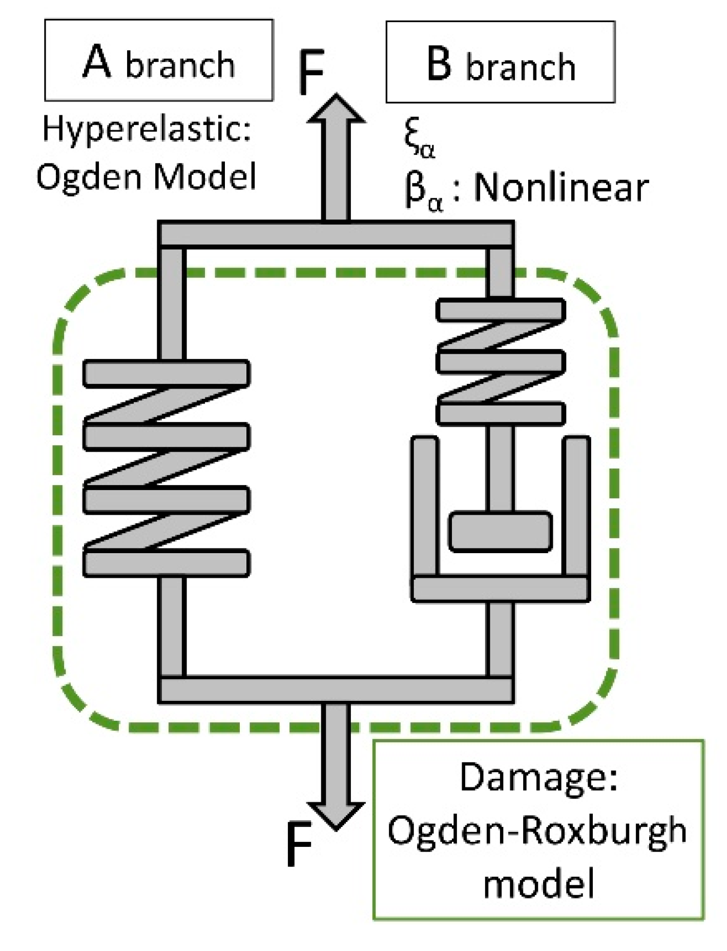
3. Proposed Visco-Hyperelastic Model with Damage

In Section 1, a brief introduction about mechanical behavior of elastomers has been exposed. As it has been said, the complex response of this kind of materials depends mainly on the strain history, the strain rate and the internal damage effect experimented by the material. To take into account all these variables a new visco-hyperelastic material model is proposed.

The parameters τ_α and β_α of the viscoelastic model described in Section 2.3 exhibit constant values. In this section, a model is presented in which only a viscoelastic branch (α = 1) is considered. The “A” branch consists of a hyperelastic spring following the Ogden model whereas the “B” branch consists of a spring and a damper in series where the β_α parameter is nonlinear. In the model described in Section 2.3 the β_α parameter has a constant value. When the model was applied to the experimental trials it became clear that there was no precise fit. It was interpreted that there could be a dependence on the actual stiffness of the material for each level of load. It was therefore decided to include this dependency in the formulation of the model. Additionally, the Ogden-Roxburgh damage model is applied to both branches, according to Figure 1.

The second Piola-Kirchhoff stress tensor is computed by Equations (9) and (13).

$${\beta }_{\alpha }=\frac{\kappa {\delta }_{\alpha } \eta }{\left(\frac{\partial \sigma }{\partial \epsilon }\right)}$$

(13)

where:

∂σ/∂ε: Tangent moduli of the hyperelastic model without damage.

η: Damage scalar parameter in Ogden-Roxburgh model.

κ: Viscoelasticity coefficient to be fitted.

δ_α: Viscoelasticity coefficient to be fitted.

The value of ∂σ/∂ε can be computed, for uniaxial tensile stress, by:

$$\frac{\partial \sigma }{\partial \epsilon }=\frac{\partial {\sigma }_1}{\partial {\lambda }_1}$$

(14)

where:

σ₁: Computed by Equation (7)

λ₁: Maximum principal stretch.

This model combines all inelastic effects that have been observed in the material experiments. The hyperelastic branch considers the non-linear behavior while the viscoelastic branch considers the strain rate. The reformulation of βα parameter allows the material behavior to be influenced by strain history and finally, all these effects are conditioned by the damage of the material during the strain cycles and that is characterized by the Mullins effect. In this work, a first experimental approach of the model is presented according to uniaxial experimental tests that are detailed below, and that are usually used in the industry to characterize these materials.

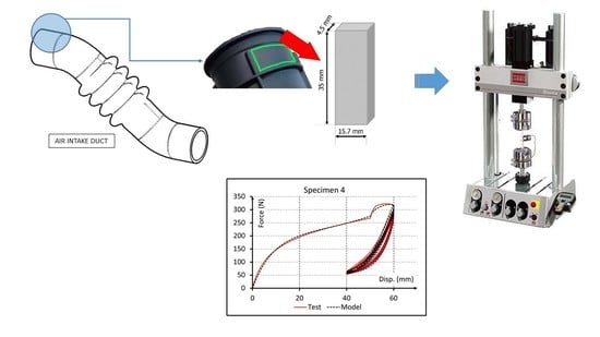
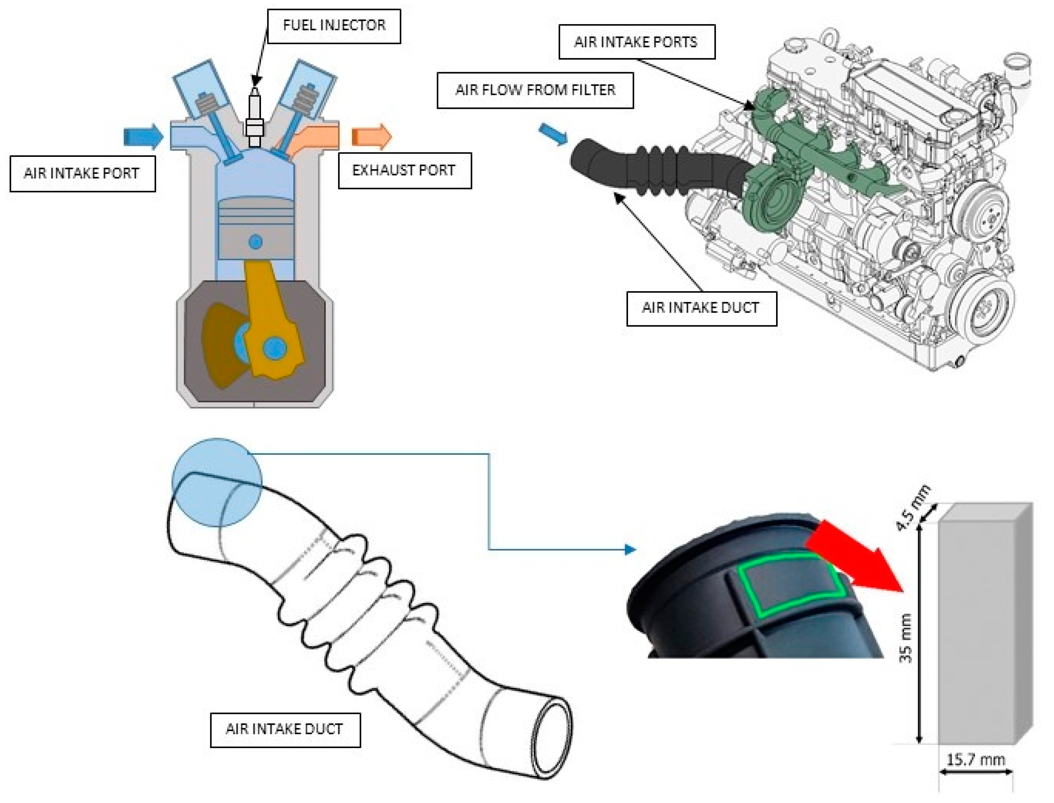
4. Experimental Tests

4.1. Material

The material used in this work is Santoprene 101-73, manufactured by Exxon Mobil. This material is used to manufacture air intake ducts for a wide range of engines assembled in well-known brands of the automotive sector (Figure 2). According to the material manufacturer, it consists of a black and versatile thermoplastic vulcanizated (TPV) and a soft thermoplastic elastomer vulcanized (TPE) [55]. The material combines good physical properties and chemical resistance for its use in a wide range of applications.

Traditional TPEs are known as two-phase composites. Essentially, a hard thermoplastic phase is chemically or mechanically coupled with a soft elastomer phase resulting in a TPE with intermediate properties between the two phases [56].

This grade of Santoprene TPV can be processed by conventional thermoplastic equipment for injection molding, extrusion, or blow molding. Based on polyolefin, it is completely recyclable [55].

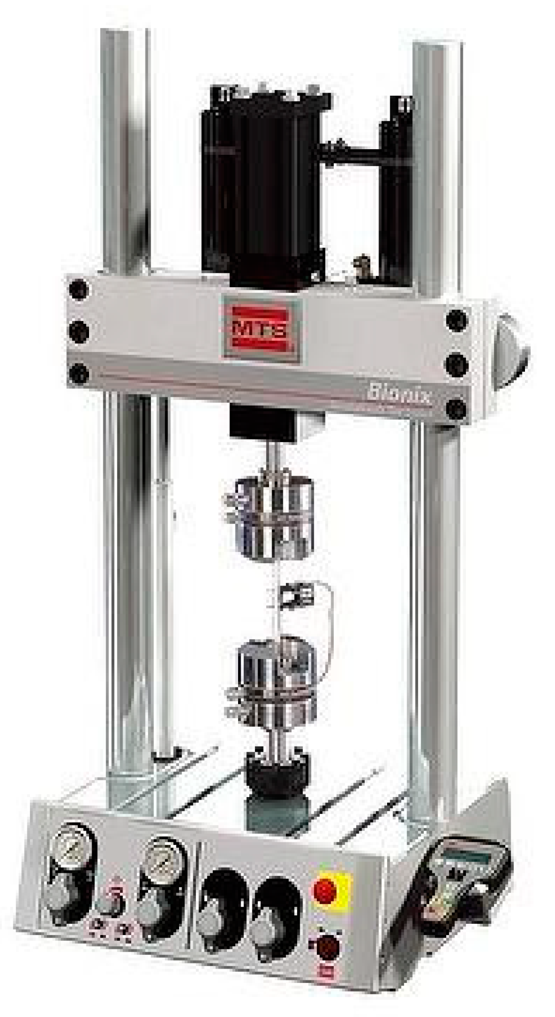
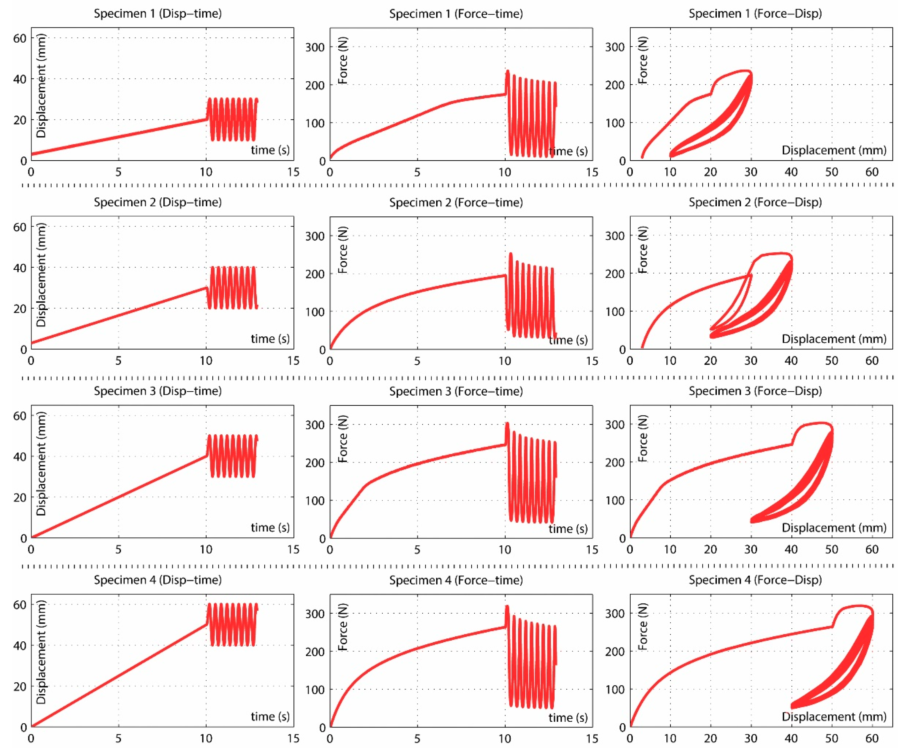
4.2. Experiments

To illustrate the visco-hyperelastic behavior and softening phenomenon of the Santoprene TPV, four cyclic uniaxial tensile tests were carried out on specimens extracted from an air duct automotive engine component. Such data are relevant because the mechanical behavior of the manufactured material, to be reproduced in this study, differs markedly from that exhibited by the virgin material as delivered by the manufacturer. This can be attributed to the manufacturing process implying notable temperature and pressure changes.

Taking into account the complex geometry of the duct component that impedes more suitable, conventional specimen shapes as “dumbbell” or “dogbone” ones [57,58,59], rectangular shaped specimens were used. The thickness, width, and length of the four specimens were 4.5 mm, 15.7 mm, and 35 mm, respectively, as shown in Figure 2.

The uniaxial tests were performed in a dynamic testing machine “Bionix Servohydraulic Test System” manufactured by MTS [60] operating in displacement control mode (Figure 3). The specimens were subjected to uniaxial cyclic tests with maximum and minimum displacements according to

Table 1. Displacements given to specimens in the experimental tests.

Samples	Displacements
	Min. Displacement	Max. Displacement
Sample 1	10 (mm)	30 (mm)
Sample 2	20 (mm)	40 (mm)
Sample 3	30 (mm)	50 (mm)
Sample 4	40 (mm)	60 (mm)

at a constant temperature of 23 °C up to 20,000 cycles (test frequency: 3 Hz).

The force and displacement were measured from data directly recorded by the testing machine. The force-displacement curves for the four specimens are presented in Figure 4, from which the following observations are drawn:

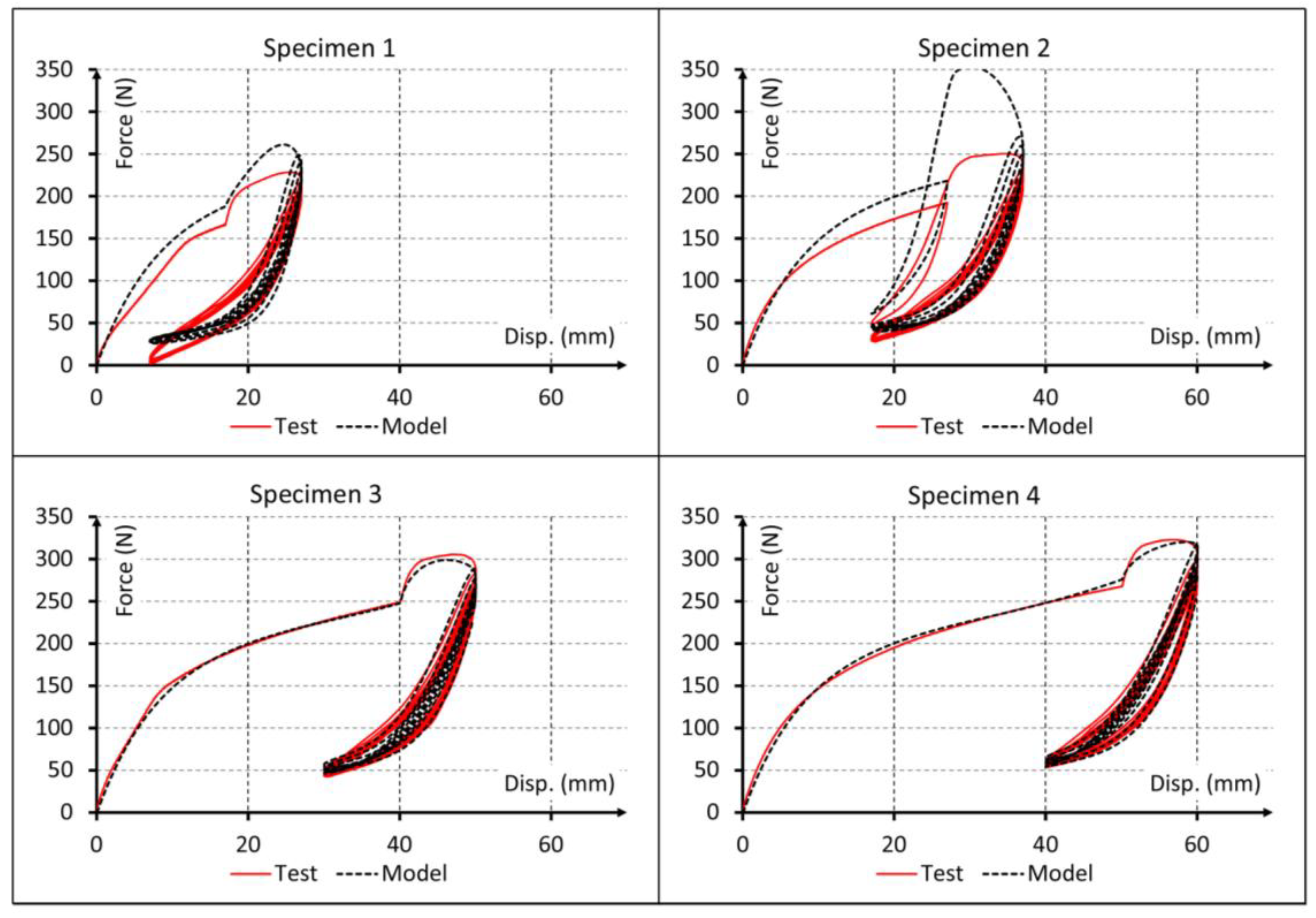
• The relation between stress and strain of the specimens in the first deformation cycle is non-linear.
• Before the maximum deformation is reached an abrupt change in the slope of the force-displacement curve is observed.
• The behavior is non-linear in subsequent cycles after the first deformation cycle.
• After the first deformation cycle, the force requested to induce the previous deformation happens to diminish notably.
• With increasing number of cycles, the applied force steadily reduces showing an asymptotic trend to a fixed value for a high number of applied cycles. Supposedly, this phenomenon can be attributed to the viscoelastic character of the material.
• Independently of the specimen tested, the force-displacement curve practically stabilizes after about 10,000 cycles.
• It follows that residual strains may induce specimens entering the plastic deformation regime.

In view of the above observations, we are able to state that the response of the Santoprene 101-73 is nonlinear and it depends on time, stress and strain history. Thus, the material behavior is driven by the hyperelastic behavior, viscoelastic behavior and Mullins effect. To reproduce the material response, the proposed numerical model, must accurately reproduce these three phenomena.

5. Fitting of Model Parameters from Experimental Data

Once the material has been characterized, all models explained in Section 2 have to be fitted with the experimental data to obtain the behavior parameters of this material [61]. The least-squares (LS) minimization method was used to identify the hyperelastic parameters in the present work. This minimization method is widely used to analyze and visualize data [62,63,64] and aims to find the minimum value of p minimizing the sum of squared errors (Equation (15)). The LS minimization method was programmed and solved in MATLAB [65].

$$p={\displaystyle \sum }_{i=1}^N{\left({\mathrm{Y}}_{\mathrm{experimental}}-{\mathrm{Y}}_{\mathrm{predicted}}\right)}_i^2$$

(15)

where N is the number of points on the chart provided by the tests.

To generalize the proposed model, it is considered that the fitting parameters process could be done in a more general way by means of metaheuristic optimization algorithms, which are adequate for solving highly non-convex and nonlinear problems [66].

5.1. Elastic Model

The Young modulus for this model is fitted by using linear least squares minimization method. The value obtained is E = 3.27 MPa.

5.2. Hyperelastic Model

To set the hyperelastic model, the Ogden N = 3 formulation was chosen. After fitting the experimental data, the resulting non-dimensional model parameters are listed in

Table 2. Ogden hyperelastic model parameter values fitted from experimental data.

Parameter	Value
μ1	11.515 (MPa)
α1	−1.979 (-)
μ2	19.930 (MPa)
α2	0.062 (-)
μ3	−27.425 (MPa)
α3	0.173 (-)

.

5.3. Visco-Hyperelastic Model

After fitting the visco-hyperelastic model to the experimental data, the model parameters listed in

Table 3. Visco-hyperelastic model parameter values fitted from experimental data.

Parameter	Value
τα	0.01 (s)
βα	−50 (-)

were obtained. They are obtained according to the fitting the model with the experimental results. However, they can be calibrated based on relaxation tests [67,68].

5.4. Ogden-Roxburgh Damage Model

To fit the damage model to the experimental data, the Roxburgh-Ogden formulation was adopted leading to the model parameters listed in

Table 4. Damage model parameter values fitted from experimental data.

Parameter	Value
r	1.338 (-)
m	0.236 (MPa)
β	0.116 (-)

.

To reproduce the force-displacement curves, Equations (1)–(12) were used by means of a numerical scheme based on displacement control as in the experimental tests for the same time step (0.01 s). The numerical scheme includes the following steps: calculation of principal stretches from test displacements values, calculation of strain energy density, parameters fitting for the hyperelastic model, calculation of stress tensor, calculation of Mullins parameter for damage and, finally, calculation of the resultant forces according to the specimen deformed dimensions. As the displacements are known at every time step, no prediction of displacements is needed, being possible to obtain all other quantities from the above equations. No problems of snapback or snapthrough were detected.

5.5. New proposed Model

As explained in Section 3, the proposed model includes a hyperelastic branch and a viscoelastic branch. The parameters used for hyperelastic branch are those specified in Table 2. It should be noted that for the viscoelastic branch the βα parameter depends on the strain history by the parameter $\raisebox{1ex}{$\partial \sigma $}\!\left/ \!\raisebox{-1ex}{$\partial \epsilon $}\right.$. The rest of viscoelastic branch parameter values are shown in

Table 5. Proposed model parameter values fitted from experimental data.

Parameter	Value
τα	0.01 (s)
δα	−50 (-)
κ	0.7 (MPa)
$\frac{\partial \sigma }{\partial \epsilon }$	Computed by Equation (14) (MPa)
η	Computed by Equation (12) (-)

. Finally, both branches of the model experience the Mullins effect by the same model and parameters specified in Section 5.4.

6. Results

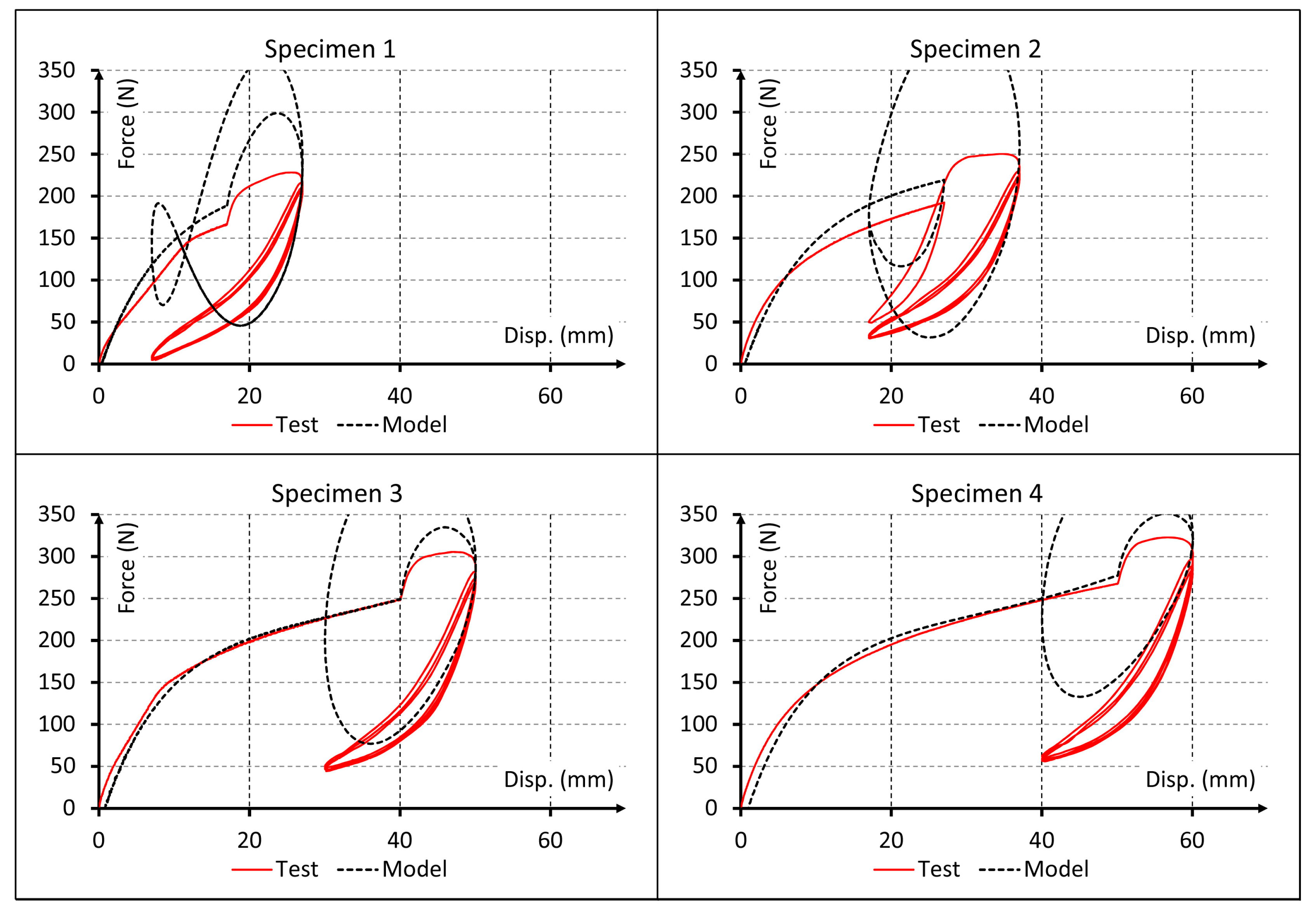
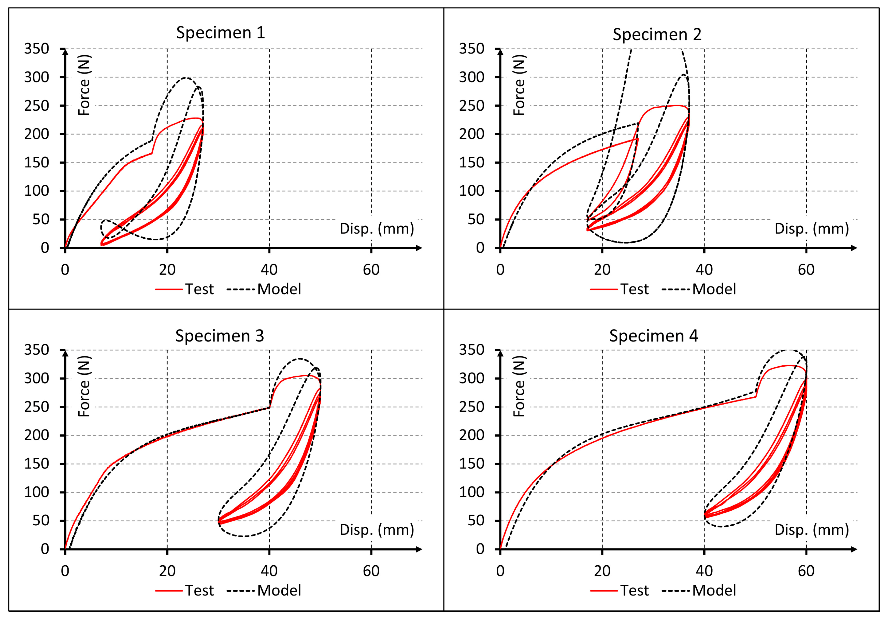
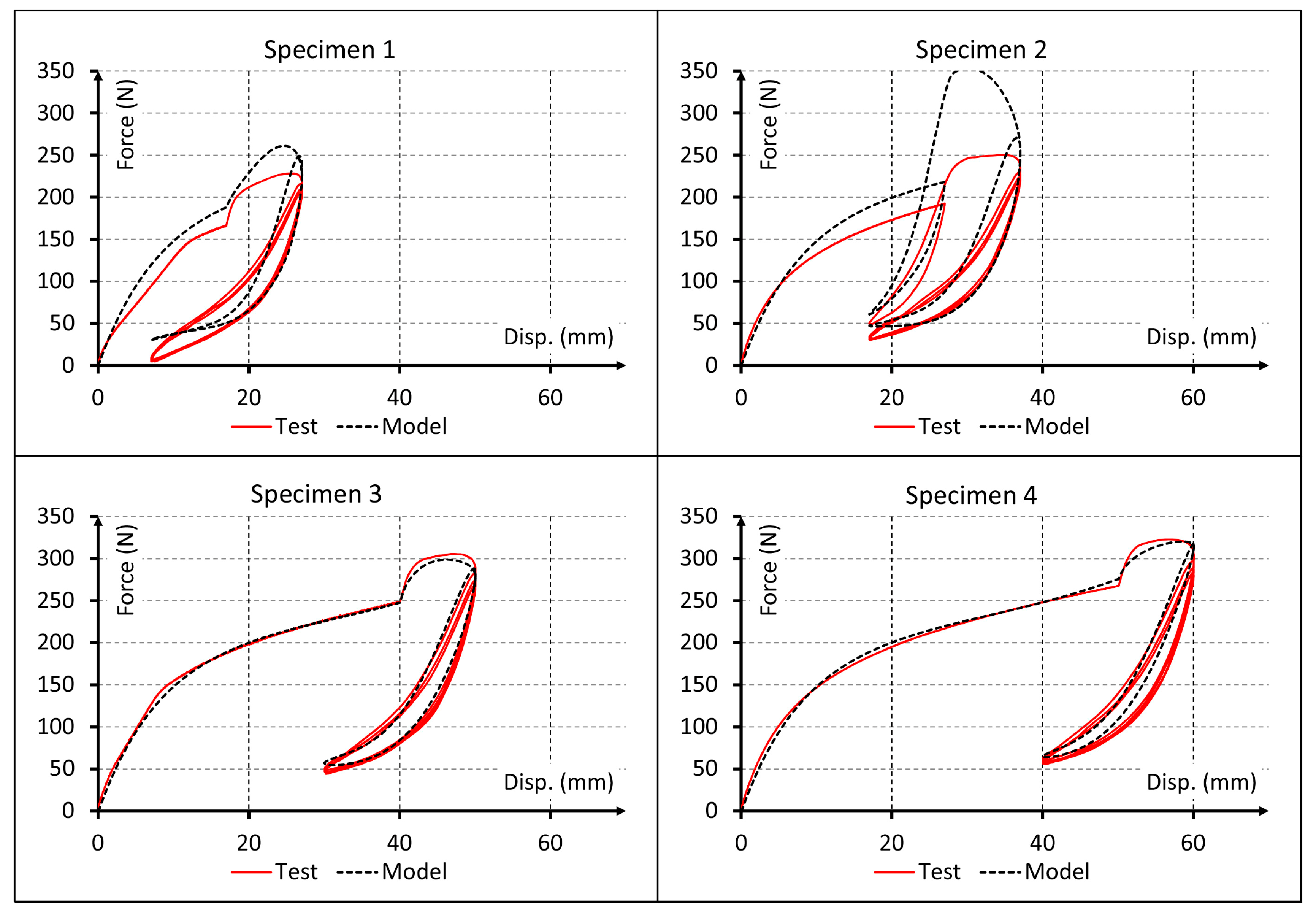
Experimental tests shown in Figure 4 were simulated according to the previously presented models:

• Linear elastic model as described in Section 2.1.
• Hyperelastic behavior, applying the Ogden model as described in Section 2.2.
• Visco-hyperelastic model as described in Section 2.2 and Section 2.3.
• Visco-hyperelastic model with Ogden-Roxburgh damage model as described in Section 2.4.
• Proposed visco-hyperelastic model with damage as described in Section 3.

Since the material behavior has clearly viscous effects, results for linear elastic and pure hyperelastic models are not plotted. Only the first cycles are represented into the plot results of Figure 5, Figure 6 and Figure 7 to obtain a proper comparison between experiments and simulations. In addition, a plot result for the proposed model and all cycles is shown in Figure 8.

Results for the visco-hyperelastic model are shown in Figure 5. In these plots the influence of viscous effects of the material can be observed but the rest of predictions are not as accurate as they could. Figure 6 shows the plot results for the visco-hyperelastic with Ogden-Roxburgh damage model explained in Section 2.4. The damage effect can be appreciated, and this improves the numerical results. These results are achieved applying models referenced in the literature, but they can be improved applying the new proposed model.

Finally, the results for the proposed model are shown in Figure 7 and Figure 8 and, visually, the numerical predictions are the best fit with test results. This is going to be checked in Section 7 using the coefficient of determination R² for all the models.

7. Discussion

To be able to analyze better the results, the coefficient of determination R² for all cases are obtained. In particular,

Table 6. Values of R² coefficient determined for each constitutive model and experimental test.

Models	Sample 1	Sample 2	Sample 3	Sample 4	Average
Elastic model	0.498	0.291	0.206	0.202	0.299
Hyperelastic model	0.539	0.371	0.331	0.316	0.389
Visco-hyperelastic model	0.548	0.400	0.347	0.348	0.411
Visco-hyperelastic with Ogden-Roxburgh damage model	0.889	0.860	0.876	0.915	0.885
Proposed model	0.972	0.979	0.986	0.976	0.978

shows the values of this coefficient calculated for each model and experimental test, as well as the average values determined for each model.

A more detailed analysis of the simulation results indicates that Model 2 reproduces the nonlinear behavior of the material and Model 3 considers the viscous behavior of the material. Both can reproduce experimental data fairly well only for the first test cycle (Figure 5). While these models could capture the start point of subsequent cyclic loading rather precisely, they completely failed to reproduce the cyclic behavior of the material. Conversely, Model 4 could capture also the early stages of the cyclic behavior of material. This improvement in results can be visually observed in Figure 7 and Figure 8 and the data of Table 6 indicate that this model provides adequate results to simulate the mechanical behavior of elastomeric materials. Finally, Model 5 captured the whole cyclic behavior better than Model 4, especially for specimens 3 and 4 (Figure 7 and Figure 8), and the R² values confirm that this model is the best of all.

The proposed visco-hyperelastic model with damage as described in Section 3 (i.e., Model 5 used in numerical simulations) allowed a satisfactory agreement to be achieved between theoretical predictions and experimental data. This is confirmed by Table 6. Since the R² coefficient computed for Model 5 was by a large extent the nearest to 1, such a model must be considered the most suited for simulating the uniaxial behavior of the tested material.

8. Conclusions

In this work, a nonlinear phenomenological visco-hyperelastic model including damage was developed to simulate the uniaxial behavior of manufactured Santoprene 101-73. The main objective pursued in this investigation was to separate the different inelastic components (hyperelasticity, viscoelasticity and damage) influencing the material behavior, thus modifying/improving relevant former models of the literature. For that purpose, a nonlinear visco-hyperelastic model was derived based on the Ogden model with damage or softening (Mullins effect).

The formulation described above was utilized to simulate cyclic uniaxial loading. Specimens were extracted from an automotive duct component made of Santoprene 101-73 and submitted to cycling loading for different displacement ranges. Optimization algorithms were used to determine the model parameter values that allow the plotting of best fit force-displacement curves resulting from experimental tests. The proposed model fitted properly the whole loading history for specimens 3 and 4, showing better results that the models found in the literature.

It must be emphasized that the fitting of force-displacement curves was done only for available uniaxial tests data. Further, thermodynamic consistency of the model has not been considered. In future work, more experimental tests are necessary, both in configuration (i.e., biaxial, volumetric, and planar) and considering different strain rates, for the complete material characterization in case of complex stress states. Moreover, a more detailed damage formulation could be incorporated in future developments to predict the material stiffness loss at high number of load cycles.

9. Future Lines of Work

This study described the first stage in the development of a new constitutive model for rubber-like materials. Authors are working on the next steps for this model and its implementation in commercial finite element software. The complete model will be a huge advance in the design of this kind of materials because models such as the proposed one allow the studying of other effects of the material from the point of view of stresses. For example, fatigue phenomena are widely studied in metallic components from this point of view, but in rubber-like materials, these phenomena must be studied focusing on strains or energies. If a good constitutive material model is developed for this kind of material, maybe, the knowledge of metal fatigue can be used to improve the current elastomer fatigue models.

References

- Dufton, P.W. Thermoplastic Elastomers; iSmithers Rapra Publishing: Akron, OH, USA, 2001. [Google Scholar]
- Delogu, M.; Del Pero, F.; Pierini, M. Lightweight design solutions in the automotive field: Environmental modelling based on fuel reduction value applied to diesel turbocharged vehicles. Sustainability 2016, 8. [Google Scholar] [CrossRef]
- Koltzenburg, S.; Maskos, M.; Nuyken, O. Elastomers. In Polymer Chemistry; Springer: Berlin, Germany, 2017; pp. 477–491. ISBN 978-3-662-49279-6. [Google Scholar]
- Rodgers, B. Rubber Compounding: Chemistry and Applications; CRC Press: Boca Raton, FL, USA, 2015. [Google Scholar]
- Yoon, S.H.; Winters, M.; Siviour, C.R. High strain-rate tensile characterization of EPDM rubber using non-equilibrium loading and the virtual fields method. Exp. Mech. 2016, 56, 25–35. [Google Scholar] [CrossRef]
- Feng, X.; Li, Z.; Wei, Y.; Chen, Y.; Kaliske, M.; Zopf, C.; Behnke, R. A novel method for constitutive characterization of the mechanical properties of uncured rubber. J. Elastom. Plast. 2016, 48, 523–534. [Google Scholar] [CrossRef]
- Bergström, J.S.; Boyce, M.C. Large strain time-dependent behaviour of filled elastomers. Mech. Mater. 2000, 32, 627–644. [Google Scholar] [CrossRef]
- Charlton, D.J.; Yang, J.; Teh, K.K. A Review of methods to characterize rubber elastic behaviour for use in finite element analysis. Rubber Chem. Technol. 1994, 67, 481–503. [Google Scholar] [CrossRef]
- Cho, H.; Mayer, S.; Pöselt, E.; Susoff, M.; in’t Veld, P.J.; Rutledge, G.C.; Boyce, M.C. Deformation mechanisms of thermoplastic elastomers: Stress-strain behaviour and constitutive modeling. Polymer 2017, 128, 87–99. [Google Scholar] [CrossRef]
- Carbary, L.D.; Kimberlain, J.H.; Oliva, J.C. Hyperelastic material model selection of structural silicone sealants for use in finite element modeling. In Proceedings of the ASME 2017 International Design Engineering Technical Conferences and Computers and Information in Engineering Conference, Cleveland, OH, USA, 6–9 August 2017; p. V001T02A001. [Google Scholar]
- Diani, J.; Fayolle, B.; Gilormini, P. A review on the Mullins effect. Eur. Polym. J. 2009, 45, 601–612. [Google Scholar] [CrossRef]
- Gil-Negrete, N.; Alonso, A. Constitutive Models for Rubber VIII; CRC Press: Boca Raton, FL, USA, 2013. [Google Scholar]
- Simulia, D. ABAQUS 6.11 Analysis User’s Manual; SIMULIA: Johnston, RI, USA, 2011; Volume 6, p. 22. [Google Scholar]
- Ogden, R.W.; Roxburgh, D.G. A pseudo-elastic model for the Mullins effect in filled rubber. Proc. R. Soc. A Math. Phys. Eng. Sci. 1999, 455, 2861–2877. [Google Scholar] [CrossRef]
- De Tommasi, D.; Ferri, D.; Marano, G.C.; Puglisi, G. Material parameters identification and experimental validation of damage models for rubberlike materials. Eur. Polym. J. 2016, 78, 302–313. [Google Scholar] [CrossRef]
- Areias, P.; Matouš, K.; Matous, K. Finite element formulation for modeling nonlinear viscoelastic elastomers. Comput. Methods Appl. Mech. Eng. 2008, 197, 4702–4717. [Google Scholar] [CrossRef]
- Arruda, E.M.; Boyce, M.C. A three-dimensional constitutive model for the large stretch behaviour of rubber elastic materials. J. Mech. Phys. Solids 1993, 41, 389–412. [Google Scholar] [CrossRef]
- Fu, Y.B.; Ogden, R.W. Nonlinear Elasticity: Theory and Applications; Cambridge University Press: Cambridge, UK, 2001; Volume 283. [Google Scholar]
- Holzapfel, G.A.; Gasser, T.C. A viscoelastic model for fiber-reinforced composites at finite strains: Continuum basis, computational aspects and applications. Comput. Methods Appl. Mech. Eng. 2001, 190, 4379–4403. [Google Scholar] [CrossRef]
- Lin, R.C. On a nonlinear viscoelastic material law at finite strain for polymers. Mech. Res. Commun. 2001, 28, 363–372. [Google Scholar] [CrossRef]
- Mooney, M. A theory of large elastic deformation. J. Appl. Phys. 1940, 11, 582–592. [Google Scholar] [CrossRef]
- Ogden, R.W. Large deformation isotropic elasticity—On the correlation of theory and experiment for incompressible rubberlike solids. Proc. R. Soc. A Math. Phys. Eng. Sci. 1972, 326, 565–584. [Google Scholar] [CrossRef]
- Rivlin, R.S. Large elastic deformations of isotropic materials. IV. Further developments of the general theory. Philos. Trans. R. Soc. A Math. Phys. Eng. Sci. 1948, 241, 379–397. [Google Scholar] [CrossRef]
- Treloar, L.R.G. The Physics of Rubber Elasticity; Oxford University Press: Cary, NC, USA, 1975. [Google Scholar]
- Yeoh, O.H. Some forms of the strain energy function for rubber. Rubber Chem. Technol. 1993, 66, 754–771. [Google Scholar] [CrossRef]
- Palacios-Pineda, L.M.; Perales-Martinez, I.A.; Lozano-Sanchez, L.M.; Martínez-Romero, O.; Puente-Córdova, J.; Segura-Cárdenas, E.; Elías-Zúñiga, A. Experimental investigation of the magnetorheological behaviour of PDMS elastomer reinforced with iron micro/nanoparticles. Polymers 2017, 9. [Google Scholar] [CrossRef]
- Tobajas, R.; Ibartz, E.; Gracia, L. A comparative study of hyperelastic constitutive models to characterize the behavior of a polymer used in automotive engines. In Proceedings of the 2nd International Electronic Conference on Materials, 2–16 May 2016; Volume 2, p. A002. [Google Scholar]
- Anani, Y.; Rahimi, G. Modeling of visco-hyperelastic behaviour of transversely isotropic functionally graded rubbers. Polym. Eng. Sci. 2016, 56, 342–347. [Google Scholar] [CrossRef]
- Jung, J.; Hwang, I.; Lee, D. Contact pressure and strain energy density of hyperelastic U-shaped monolithic seals under axial and radial compressions in an insulating joint: A numerical study. Appl. Sci. 2017, 7, 792. [Google Scholar] [CrossRef]
- Breche, Q.; Chagnon, G.; Machado, G.; Nottelet, B.; Garric, X.; Girard, E.; Favier, D. A non-linear viscoelastic model to describe the mechanical behaviour’s evolution of biodegradable polymers during hydrolytic degradation. Polym. Degrad. Stab. 2016, 131, 145–156. [Google Scholar] [CrossRef]
- Wu, Y.; Wang, H.; Li, A. Parameter identification methods for hyperelastic and hyper-viscoelastic models. Appl. Sci. 2016, 6, 386. [Google Scholar] [CrossRef]
- Nguyen, V.D.; Lani, F.; Pardoen, T.; Morelle, X.P.; Noels, L. A large strain hyperelastic viscoelastic-viscoplastic-damage constitutive model based on a multi-mechanism non-local damage continuum for amorphous glassy polymers. Int. J. Solids Struct. 2016, 96, 192–216. [Google Scholar] [CrossRef]
- Ward, I.; Sweeney, J. Mechanical Properties of Solid Polymers; John Wiley & Sons: Hoboken, NJ, USA, 2012; Volume 13, ISBN 9038628064. [Google Scholar]
- Bai, Y.; Liu, C.; Huang, G.; Li, W.; Feng, S. A hyper-viscoelastic constitutive model for polyurea under uniaxial compressive loading. Polymers 2016, 8, 133. [Google Scholar] [CrossRef]
- Bonfitto, A.; Tonoli, A.; Amati, N. Viscoelastic dampers for rotors: Modeling and validation at component and system level. Appl. Sci. 2017, 7, 1181. [Google Scholar] [CrossRef]
- Aboudi, J. The effect of evolving damage on the finite strain response of inelastic and viscoelastic composites. Materials 2009, 2, 1858–1894. [Google Scholar] [CrossRef]
- Bolotin, V.V. Prediction of Service Life for Machines and Structures; American Society of Mechanical Engineers: New York, NY, USA, 1988. [Google Scholar]
- Grandcoin, J.; Boukamel, A.; Lejeunes, S. A micro-mechanically based continuum damage model for fatigue life prediction of filled rubbers. Int. J. Solids Struct. 2014, 51, 1274–1286. [Google Scholar] [CrossRef]
- De Tommasi, D.; Puglisi, G.; Saccomandi, G. A micromechanics-based model for the Mullins effect. J. Rheol. 2006, 50, 495–512. [Google Scholar] [CrossRef]
- Schapery, R.A. A micromechanical model for non-linear viscoelastic behaviour of particle-reinforced rubber with distributed damage. Eng. Fract. Mech. 1986, 25, 845–867. [Google Scholar] [CrossRef]
- Drozdov, A.D.; Dorfmann, A. A micro-mechanical model for the response of filled elastomers at finite strains. Int. J. Plast. 2003, 19, 1037–1067. [Google Scholar] [CrossRef]
- Mullins, L. Softening of rubber by deformation. Rubber Chem. Technol. 1969, 42, 339–362. [Google Scholar] [CrossRef]
- Miñano, M.; Montáns, F.J. A new approach to modeling isotropic damage for Mullins effect in hyperelastic materials. Int. J. Solids Struct. 2015, 67–68, 272–282. [Google Scholar] [CrossRef]
- Andriyana, A.; Loo, M.S.; Chagnon, G.; Verron, E.; Ch’ng, S.Y. Modeling the Mullins effect in elastomers swollen by palm biodiesel. Int. J. Eng. Sci. 2015, 95, 1–22. [Google Scholar] [CrossRef]
- Setiyana, B.; Wicahyo, F.D.; Ismail, R.; Jamari, J.; Schipper, D.J. Investigation on the elastic modulus of rubber-like materials by straight blade indentation using numerical analysis. Adv. Mater. Res. 2015, 1123, 55–58. [Google Scholar] [CrossRef]
- Li, Z.; Zhou, Z.; Li, Y.; Tang, S. Effect of cyclic loading on surface instability of silicone rubber under compression. Polymers 2017, 9, 148. [Google Scholar] [CrossRef]
- Safshekan, F.; Tafazzoli-Shadpour, M.; Abdouss, M.; Shadmehr, M.B. Mechanical characterization and constitutive modeling of human trachea: Age and gender dependency. Materials 2016, 9, 456. [Google Scholar] [CrossRef] [PubMed]
- Liao, B.; Sun, B.; Yan, M.; Ren, Y.; Zhang, W.; Zhou, K. Time-variant reliability analysis for rubber O-ring seal considering both material degradation and random load. Materials 2017, 10, 1211. [Google Scholar] [CrossRef] [PubMed]
- Felipe-Sesé, L.; López-Alba, E.; Hannemann, B.; Schmeer, S.; Diaz, F.A. A validation approach for quasistatic numerical/experimental indentation analysis in soft materials using 3D digital image correlation. Materials 2017, 10, 722. [Google Scholar] [CrossRef] [PubMed]
- Uriarte, I.; Zulueta, E.; Guraya, T.; Arsuaga, M.; Garitaonandia, I.; Arriaga, A. Characterization of recycled rubber using particle swarm optimization techniques. Rubber Chem. Technol. 2015, 88, 343–358. [Google Scholar] [CrossRef]
- Liu, C.; Cady, C.M.; Lovato, M.L.; Orler, E.B. Uniaxial tension of thin rubber liner sheets and hyperelastic model investigation. J. Mater. Sci. 2015, 50, 1401–1411. [Google Scholar] [CrossRef]
- Horgan, C.O. The remarkable Gent constitutive model for hyperelastic materials. Int. J. Non Linear Mech. 2015, 68, 9–16. [Google Scholar] [CrossRef]
- Hariharaputhiran, H.; Saravanan, U. A new set of biaxial and uniaxial experiments on vulcanized rubber and attempts at modeling it using classical hyperelastic models. Mech. Mater. 2016, 92, 211–222. [Google Scholar] [CrossRef]
- Fahimi, S.; Baghani, M.; Zakerzadeh, M.-R.; Eskandari, A. Developing a visco-hyperelastic material model for 3D finite deformation of elastomers. Finite Elem. Anal. Des. 2018, 140, 1–10. [Google Scholar] [CrossRef]
- Exxon Mobil Technical Datasheet: Santoprene 101-73 Thermoplastic Vulcanizate 2014; Mobil: Irving, TX, USA, 2014.
- Whelan, A. Polymer Technology Dictionary; Springer Science & Business Media: Berlin, Germany, 2012. [Google Scholar]
- Chandima Chathuranga Somarathna, H.M.; Raman, S.N.; Badri, K.H.; Mutalib, A.A.; Mohotti, D.; Ravana, S.D. Quasi-static behaviour of palm-based elastomeric polyurethane: For strengthening application of structures under impulsive loadings. Polymers 2016, 8, 202. [Google Scholar] [CrossRef]
- Piesowicz, E.; Paszkiewicz, S.; Szymczyk, A. Phase separation and elastic properties of poly(trimethylene terephthalate)-blockpoly(ethylene oxide) copolymers. Polymers 2016, 8, 237. [Google Scholar] [CrossRef]
- Luo, R.K.; Zhou, X.; Tang, J. Numerical prediction and experiment on rubber creep and stress relaxation using time-dependent hyperelastic approach. Polym. Test. 2016, 52, 246–253. [Google Scholar] [CrossRef]
- MTS System Corporation. Available online: http://www.mts.com/en/index.htm (accessed on 19 March 2018).
- Beda, T. An approach for hyperelastic model-building and parameters estimation a review of constitutive models. Eur. Polym. J. 2014, 50, 97–108. [Google Scholar] [CrossRef]
- Mihai, L.A.; Budday, S.; Holzapfel, G.A.; Kuhl, E.; Goriely, A. A family of hyperelastic models for human brain tissue. J. Mech. Phys. Solids 2017, 106, 60–79. [Google Scholar] [CrossRef]
- Stumpf, F.T.; Marczak, R.J. Characterization of constitutive parameters for hyperelastic models considering the Baker-Ericksen inequalities. In Advanced Structured Materials; CRC Press: Boca Raton, FL, USA, 2016; Volume 49, pp. 375–393. [Google Scholar]
- Balaban, G.; Alnæs, M.S.; Sundnes, J.; Rognes, M.E. Adjoint multi-start-based estimation of cardiac hyperelastic material parameters using shear data. Biomech. Model. Mechanobiol. 2016, 15, 1509–1521. [Google Scholar] [CrossRef] [PubMed]
- MATLAB and Statistics Toolbox; The MathWorks Inc.: Natick, MA, USA, 2010; ISBN 0885-7458.
- Pelteret, J.P.; Walter, B.; Steinmann, P. Application of metaheuristic algorithms to the identification of nonlinear magneto-viscoelastic constitutive parameters. J. Magn. Magn. Mater. 2018, 464, 116–131. [Google Scholar] [CrossRef]
- Pawlikowski, M. Non-linear constitutive model for the oligocarbonate polyurethane material. Chin. J. Polym. Sci. (Engl. Ed.) 2014, 32, 1666–1677. [Google Scholar] [CrossRef]
- Goh, S.M.; Charalambides, M.N.; Williams, J.G. Determination of the constitutive constants of non-linear viscoelastic materials. Mech. Time-Depend. Mater. 2004, 8, 255–268. [Google Scholar] [CrossRef]