Accurate Estimation of Brittle Fracture Toughness Deterioration in Steel Structures Subjected to Large Complicated Prestrains

Abstract

Studies have suggested that brittle fractures occur in steel because microcracks in the brittle layer at grain boundaries propagate as a result of the increase in piled-up dislocations. Therefore, prestraining can approach the limits of a material, which could lead to a decrease in fracture toughness. However, strains are tensors comprising multiple components, so the effect of prestrain on fracture toughness is not simple. Additionally, the mechanism of change in critical stress due to prestrain has not been thoroughly investigated. For the lifetime evaluation of steel structures with a complicated load history, it is important to generalize the effect of complicated prestrain on the decrease in fracture toughness. In this paper, a single prestrain was applied in a direction different from the crack opening direction. A general three-point bending test was employed for fracture evaluation. Numerical analyses using the strain gradient plasticity (SGP) theory, which is a method based on the finite element method (FEM) are carried out; conventional macroscopic material damage rules are considered as well. Using these FEM analyses, the critical stress is calculated. Finally, the change in critical stress can be expressed by the yield point increase and dislocation density and formulated based on the identified micromechanisms.

1. Introduction

Iron is the most abundant element on earth and is used in many applications, including high-rise buildings, large structures, infrastructure (e.g., pipelines for transporting natural gas and storage tanks for natural gas), and ships. As the size of these structures continues to increase, the risk of brittle fractures steadily increases. However, brittle fractures are intrinsically inevitable in carbon steel material due to its lattice structure. To ensure the safety of steel structures by preventing brittle fractures, a deeper understanding of brittle fractures is required.

To begin this study, the historical aspects of the mechanisms of brittle fracture in steel are introduced. Brittle fractures are considered to originate from a microcrack in a heterogeneous microstructure. The most famous governing formula that combines microcracks and fractures is Griffith’s equation, which is shown in Equation (1) [1]:

$${\sigma }_{\mathrm{f}}=\sqrt{\frac{2E\gamma }{\pi c}}$$

(1)

where ${\sigma }_{\mathrm{f}}$is the critical stress, $E$ is the Young’s modulus, $\gamma$ is the surface energy per unit area, and $c$ is the crack length. Equation (1) is derived based on the second law of thermodynamics and Inglis’s solution [2] and indicates that a cleavage fracture occurs due to crack propagation when the stress exceeds ${\sigma }_{\mathrm{f}}$. However, this critical stress observed in practice is much lower than the theoretical fracture strength. Therefore, different influential mechanisms on the actual fracture in steel have been investigated. Stroh [3] suggested that piled-up dislocations from plastic deformation affected the fracture. Later, this theory was applied to Smith’s [4] and Petch’s equation [5,6]. Smith [4] suggested that the critical stress is greatly affected by the thickness of carbide particles at the grain boundaries and formulated the critical condition as follows:

$${\sigma }_{\mathrm{f}}=\sqrt{\frac{4E{\gamma }_{\mathrm{p}}}{\pi t}-{\left\{{\tau }_{\mathrm{eff}}\sqrt{\frac{d}{t}}+\frac{4{\tau }_i}{\pi }\right\}}^2}$$

(2)

where ${\gamma }_{\mathrm{p}}$ is the plastic work required to create a unit area of fracture surface, ${\tau }_{\mathrm{eff}}$ is the effective shear stress, $d$ is the grain diameter, $t$ is the thickness of the carbide layer, and ${\tau }_i$ is the frictional stress. This equation is based on experimental results, which showed that brittle cracks always initiated by the occurrence of microcracks in the brittle layer, such as carbide particles located in grain boundaries, as shown in Figure 1.

As shown in Figure 1, the dislocation motion is generated by plastic deformation, and the dislocations pile up to the carbide layer as a result of shear stress when tensile stress is applied at a distance. The piled-up dislocations create a stress concentration at the carbide layer, which induces the nucleation of a microcrack. The mechanism of brittle fracture is the nucleation and propagation of the brittle crack, which initiates in the carbide layer.

Petch [5,6] improved this concept using major microstructural parameters, yield stress and grain diameter and proposed a practical formula that is dominated by the nucleation of microcracks. On the basis of dislocation theory, Cottrell [7] suggested that the critical conditions for cleavage fracture are determined not only by the nucleation of microcracks but also by the growth of the microcracks.

Using these models, a number of application studies of critical stress have been carried out over many years. Based on the knowledge that brittle fractures occur according to the weakest link model [8], the Weibull stress model was proposed by Beremin [9]. This theory states that the critical condition can be accurately estimated by using the probability of microcrack existence, which is determined with Griffith’s equation. A number of studies have been carried out based on the Beremin model. Bordet [10,11] postulated that the nucleation and growth of microcracks can be treated independently. In recent studies, Lei [12,13] suggested that an improvement in accuracy can be made by reconsidering the Weibull stress model based on the experience that brittle cracks never occur without yielding. However, there are some mandatory parameters that are difficult to determine in this improved model, which makes it difficult to apply this model in actual engineering applications.

In addition to these approaches purely regarding the critical stress condition of the material itself, a number of studies of critical stress after prestraining have been investigated. Based on Smith’s model, plastic deformation leads to an increase in piled-up dislocations and directly results in an increase in the risk of brittle fracture. Actually, microcrack nucleation induced by plastic deformation was recognized in experimental observations [14,15]. Therefore, subjecting a material to plastic prestrain means getting close to the limit of the material and leading to a decrease in fracture toughness. Some previous works have focused on the effect of prestrain on fracture toughness. Sukedai et al. [16] showed that the fracture toughness of Charpy impact test samples decreased when the samples were subjected to a tensile prestrain. Miki et al. [17] showed that critical crack tip opening displacement (CTOD) decreased when a sample was subjected to either tensile or compressive prestrains. From their experimental results, they verified that a single prestrain led to a decrease in fracture toughness. However, strain is a tensor comprising multiple components, which makes it difficult to understand the effects of prestrain. The generalized effects of prestrain, including cyclic or directional prestrain, have not been quantitatively elaborated. Although many structural members are subjected to complicated strain cycles, such as simple uniaxial tensile-compressive strain cycles and multidirectional strain cycles, where the crack opening direction is different, a sufficient mechanism of toughness deterioration has not been discovered. Recently, Kosuge et al. [18] revealed the effects of random tensile-compressive uniaxial prestrain on the ductile–brittle transition temperature (DBTT) through experiments and finite element method (FEM) analyses, which included the effects of piled-up dislocations. They showed that the relationship between the number of piled-up dislocations and the amount of shift in the DBTT of a fracture toughness test sample has a one-to-one correspondence. Hence, it is clear that, regarding toughness degradation under plastic prestrains, the number of piled-up dislocations is the main factor that controls brittle fracture performance. However, this relationship is effective only for one fracture toughness specimen configuration, so generalization to actual steel structures is necessary.

Different practical studies combining experiments and numerical analyses reported that the critical stress increased [19], decreased [20], or remained constant [21] after prestraining. Therefore, it is reasonable to assume that the critical stress is affected by prestrain in some way, but the mechanism by which the critical stress is affected under different prestraining conditions has not been clarified because sufficient knowledge has not been obtained. Critical stress is very important for determining the occurrence of brittle fractures because the stress distribution at the crack tip can be easily calculated with commercial FEM software. To predict and prevent catastrophic brittle fractures, the effect of prestrain on the change in critical stress must be thoroughly understood because most structures are subjected to complicated strain histories (e.g., earthquakes for on-land structures and heavy wave impacts for offshore structures).

In this paper, based on the abovementioned background, the change in critical stress under various prestraining conditions was investigated by combining experiments and numerical analyses. The effect of the prestrain direction was investigated by applying the prestrain in a different direction than the crack opening direction. The critical stress was determined using FEM analysis, and the results were compared according to the prestrain direction. Additionally, FEM analysis based on crystal plasticity was conducted to examine the mechanism in more detail and to formulate the generalized effect of prestrain on critical stress.

2. Experiment

In this section, the methods used in this study for prestraining and fracture testing are presented and the results from these tests are explained. The effect of the prestrain direction was evaluated by implementing four different prestrain directions.

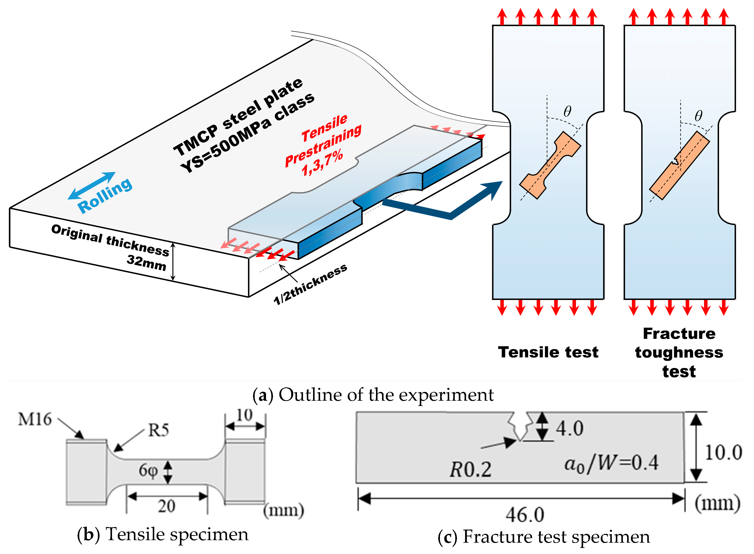
2.1. Preparation of Testing and Prestraining

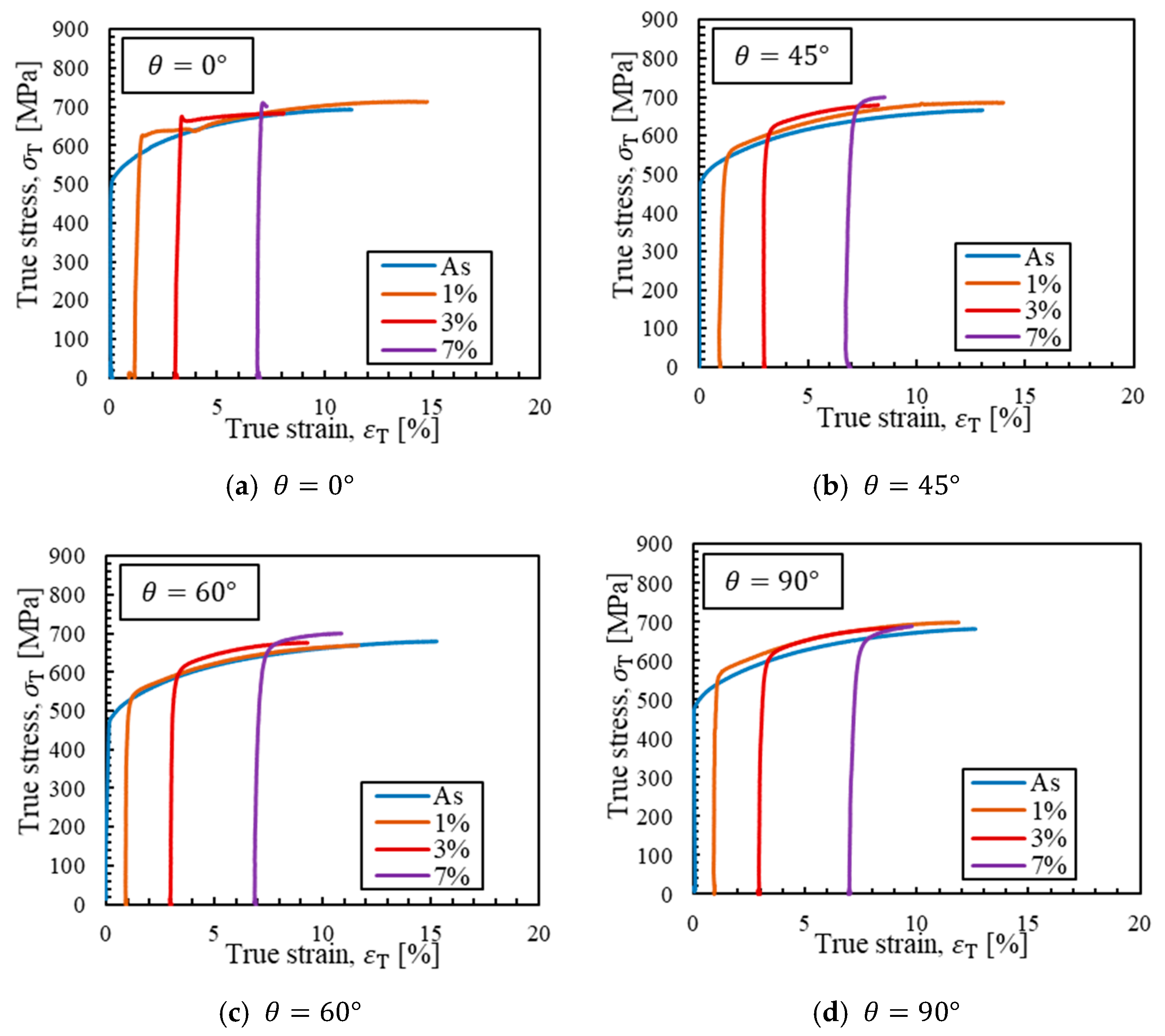
In this research, a thermomechanical control process (TMCP) steel plate [22] with a thickness of 32 mm was used. TMCP steel is applied in various fields, such as natural gas pipelines [23], offshore structures [24], tanks [25], ships [26], buildings [27], and bridges [28]. The yield strength and tensile strength of the TMCP steel in this study are about 500 MPa and 600 MPa, respectively. The test specimens subjected to prestraining were machined from the mid-thickness position so that the longitudinal direction was vertical to the rolling direction, as shown in Figure 2a. The selected amounts of prestrain were 1%, 3%, and 7%, which were measured as the change in the gage length distance. To investigate the effect of the prestrain on the yield stress or uniform elongation, a tensile test was carried out using round bar test specimens after applying the prestrain depicted in Figure 2b. Additionally, the main mode of evaluation in this study, the fracture toughness test, was performed using three-point bending specimens, as shown in Figure 2c. There were no fatigue precracks at the tip of the notch, and only a sharp notch shape remained. Regarding both specimens, the important parameter, $\theta$, is defined as the angle between the prestrain direction and the longitudinal direction of the specimen, and $\theta$ was changed to $0°, 45°, 60° \mathrm{and} 90°$.

2.2. Tensile Tests

True stress-true strain curves calculated from the experiment are shown in Figure 3. After applying the prestrain, the curves shifted to the right according to the amount of prestrain. As shown in Figure 3, strain hardening by prestraining was observed at all angles, wherein the yield stress increased and uniform elongation decreased. Additionally, the shape of the curve did not change significantly, indicating that the aging had little effect on the samples.

2.3. Fracture Test

Three specimens were prepared for each prestrain condition, and a general three-point bending test was carried out at −160 °C. To observe the effect of prestrain on fracture toughness, fracture test specimens with no prestrain were also prepared. Additionally, the TMCP steel plate generally has strong anisotropy due to the growth of texture created during the unrecrystallization temperature range, so the fracture toughness is considered to be different in each direction. Thus, specimens without prestrain were prepared in four directions ($\theta =0°, 45°, 60° \mathrm{and} 90°,$and especially $\theta =0°$ is vertical and $\theta =90°$ is parallel to rolling direction). As mentioned in Section 2.1, this specimen does not have fatigue cracks, so this test cannot be regarded as a CTOD test, which is specified in the International Organization for Standardization (ISO) standard [29]. Therefore, the CTOD obtained from this experiment is denoted as “quasi-CTOD” hereinafter and is distinguished from the standardized CTOD. However, quasi-CTOD was calculated by Equations (3)–(9) [30,31].

$${\delta }_{\mathrm{quasi}.\mathrm{cr}}=\frac{K^2}{m{\sigma }_{\mathrm{y}}E}+f_{\mathrm{p}}\frac{r_{\mathrm{p}}\left(W-a_0\right)}{r_{\mathrm{p}}\left(W-a_0\right)+a_0+z}{V}_{\mathrm{p}}$$

(3)

$$m=4.9-3.5YR$$

(4)

$$r_{\mathrm{p}}=0.43$$

(5)

$$f_p=F\left(B\right)·f_{\mathrm{p}@\mathrm{B}=25 mm}\left(YR\right)$$

(6)

$$f\left(\frac{a_0}{W}\right)=\frac{3{\left(\frac{a_0}{W}\right)}^{\frac{1}{2}}[1.99-\left(\frac{a_0}{W}\right)\left(1-\frac{a_0}{W}\right)\left(2.15-3.93\frac{a_0}{W}+2.7{\left(\frac{a_0}{W}\right)}^2\right]}{2\left(1+2\frac{a_0}{W}\right){\left(1-\frac{a_0}{W}\right)}^{\frac{3}{2}}}$$

(7)

$$F\left(B\right)=0.8+0.2\exp \left\{-0.019\left(B-25\right)\right\}$$

(8)

$$f_{\mathrm{p}@\mathrm{B}=25 \mathrm{mm}}\left(YR\right)=-1.4{\left(YR\right)}^2+2.8\left(YR\right)-0.35$$

(9)

where $m$ is the constraint factor, $K$ is the stress intensity factor, $f_p$ is the plasticity correction factor, $a_0$ is the initial crack length, $W$ is the width, $B$ is the thickness, ${\sigma }_{\mathrm{y}}$ is the yield stress, $YR$ is the yield ratio, $V_{\mathrm{p}}$ is the plastic displacement of the clip gage, and ${\delta }_{\mathrm{quasi}.\mathrm{cr}}$ is the “quasi-CTOD”. In this test, material constants were given as shown in

Table 1. Value of each parameter in the equations used for crack tip opening displacement (CTOD) calculations.

Parameter	Value	Units
${\sigma }_{\mathrm{y}}$	500	MPa
E	206	GPa
YR	0.806	-
B	10	mm
W	10	mm
$a_0$	4	mm
S	80	mm
z	−1.5	mm

.

According to the experimental data, ${\delta }_{\mathrm{quasi}.\mathrm{cr}}$ was calculated using these equations and was compared for each prestrain condition, as shown in Figure 4. The vertical axis of Figure 4 shows the nondimensional toughness variation index ${\delta }_{\mathrm{quasi}.\mathrm{cr}}$ (after prestraining) divided by ${\delta }_{\mathrm{quasi}.\mathrm{cr}\_\mathrm{As}}$ (with no prestrain) for each direction. As shown in Figure 4, the samples exhibit remarkable embrittlement in all prestrain conditions, although there was a difference depending on the angle.

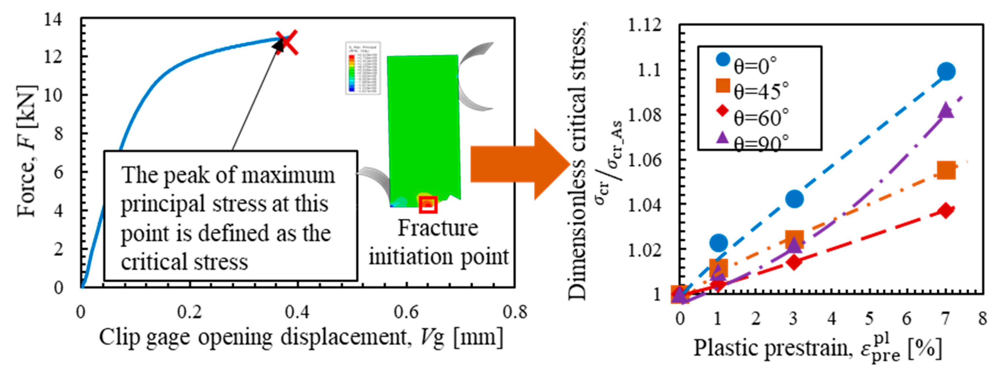
3. Calculation of Critical Stress

In this section, the critical stress was calculated based on the experimental results shown in the previous section. FEM analysis was carried out as a continuous simulation covering all processes, including prestraining and fracture tests. Finally, the critical stress was obtained for each experiment, and the results were compared among the different prestrain conditions.

3.1. Simulation of the Prestraining Process

In this analysis, a combined hardening rule, which combines isotropic and kinematic hardening rules, was used for the simulation. The steel material undergoes strain hardening with plastic deformation and yield surface changes. The isotropic hardening rule defines the magnitude of the yield surface, and the kinematic hardening rule represents the movement of the yield surface. In this study, because the prestrain direction was different from the crack opening direction, the Bauschinger effect was considered to be undergoing load reversal. In the case where load reversal occurs, the yield surface moves while changing its magnitude, so the combined hardening rule is considered to be appropriate. The combined hardening rule is defined in Equations (10) and (11).

$${\sigma }^0=\sigma {|}_0+Q_{\infty }\left(1-e^{-\beta {\overline{\epsilon }}^{\mathrm{pl}}}\right)$$

(10)

$${\dot{\alpha }}_{ij}=C\frac{1}{{\sigma }^0}\left({\sigma }_{ij}-{\alpha }_{ij}\right){\dot{\overline{\epsilon }}}^{\mathrm{pl}}-\gamma {\alpha }_{ij}{\dot{\overline{\epsilon }}}^{\mathrm{pl}}$$

(11)

Isotropic hardening is expressed by Equation (10) [32], whereas kinematic hardening is expressed by Equation (11) [33]. In these equations, ${\sigma }^0$ is the equivalent stress that decides the magnitude of the yield surface, $\sigma {|}_0$ is the yield stress with no plastic strain, $Q_{\infty } \mathrm{and} \beta$ are intrinsic material parameters, $C$ is the initial kinematic hardening coefficient, and $\gamma$ is the parameter that expresses the damping factor of the kinematic hardening coefficient. In this analysis, each parameter was determined by trial-and-error, as shown in

Table 2. Determination of the parameters in the combined hardening rule.

Parameter	Value	Units
$\sigma {|}_0$	500	MPa
$Q_{\infty }$	200	MPa
$\beta$	4.5	-
C	10,000	MPa
$\mathsf{\gamma }$	81	-

.

3.2. Simulation of the Fracture Test

A three-point bending test for evaluating fracture toughness was simulated with an FEM model. Similar to the simulation of the prestraining process, the combined hardening rule was applied in this step. In this analysis, the “Map Solution” technique [34] was used to transfer all analysis results, including the back stress tensor and plastic strain from the prestraining simulation, to the initial conditions of the fracture test model, which has completely different mesh divisions. Then, the fracture test can be simulated, including the parameters of plastic strain and back stress from the prestraining simulation. The prestrain direction can be arbitrarily reproduced by rotating the model during mapping from the prestraining process to the fracture test simulation. In the fracture test process, the combined hardening parameters were optimized for each angle condition, as shown in

Table 3. Determination of the parameters for the fracture test.

Parameter	$\mathit{\theta }=0°$	$\mathit{\theta }=45°$	$\mathit{\theta }=60°$	$\mathit{\theta }=90°$	Units
$\sigma {|}_0$	750	750	750	750	MPa
$Q_{\infty }$	500	600	500	550	MPa
$\beta$	3	3	3	3	-
C	5000	5000	5000	5000	MPa
$\mathsf{\gamma }$	81	81	81	81	-

, to accurately estimate the stress–strain relationship after prestraining. Using these parameters, a full process analysis including the prestraining process and the subsequent fracture test was carried out.

Next, the critical stress was calculated based on the analysis mentioned above. As shown in Figure 5, the representative fracture initiation point was regarded as the point with the largest value of maximum principal stress at the time when the bending test specimen fractured. Under this assumption, the maximum principal stress at the fracture point was regarded as the critical stress. The largest value of maximum principal stress appeared near the notch root on the mid-thickness plane. The critical stress was calculated under all prestrain conditions, including the “As” condition (without prestraining). Figure 5 shows the change in the critical stress under each prestrain condition. The critical stress without prestrain, ${\sigma }_{\mathrm{cr}\_\mathrm{As}}$, was different from the critical stress with prestrain in different directions. Therefore, the critical stress after prestrain, ${\sigma }_{\mathrm{cr}}$, was made dimensionless through a comparison with ${\sigma }_{\mathrm{cr}\_\mathrm{As}}$. As shown in Figure 5, the critical stress tended to increase with the increase in prestrain under all prestrain directions, and the ratio of the increase varies with respect to the prestrain direction. Based on these results, the mechanism of the increase in the critical stress was investigated from the viewpoint of both the continuum macroscopic model and the crystal plasticity model in the next section.

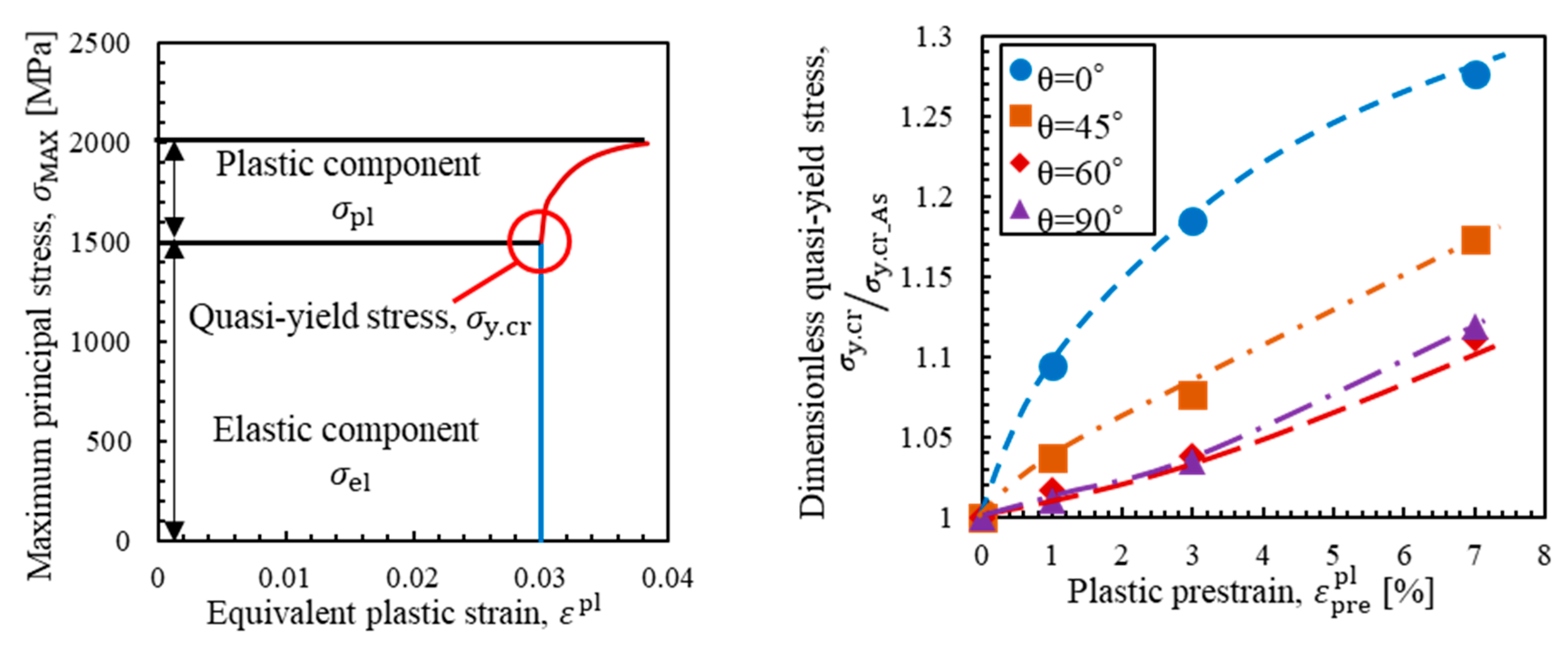
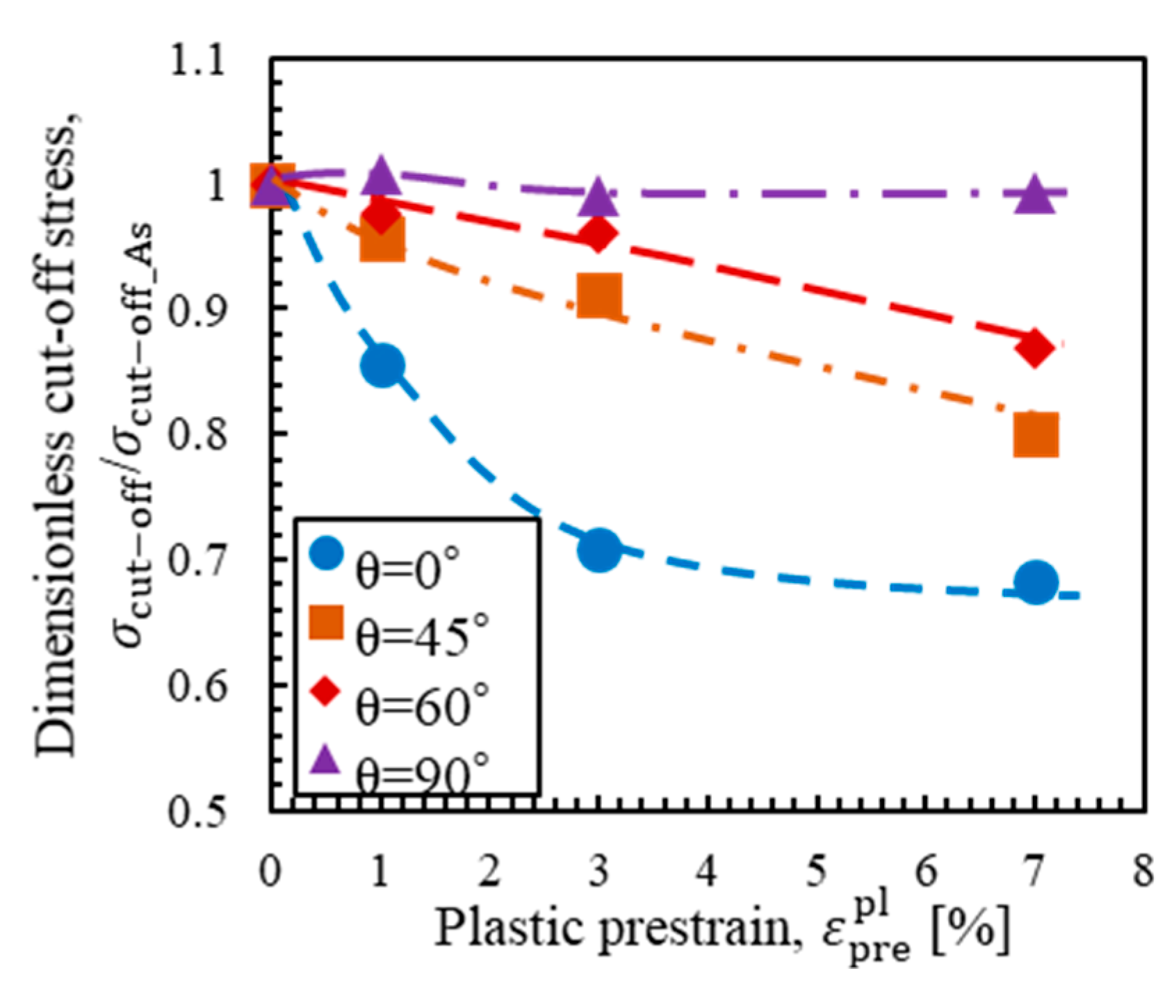
4. Mechanism of Change in Critical Stress

In the previous section, it was revealed that the critical stress clearly increased with respect to the amount of prestrain. The increase ratio varied with respect to the prestrain direction. Hence, to evaluate the safety of structures, it is important to understand how the critical conditions change when a complicated prestrain is applied, and the mechanism that can explain the experimental results should be investigated in detail. In this section, the critical stress change mechanism is clarified based on both the continuum macroscopic model and the crystal plasticity model.

4.1. Analysis of the Macroscopic Model

In this subsection, the candidate mechanism is investigated based on a macroscopic model. It is reasonable that material damage progresses by plastic deformation and does not occur during elastic deformation [12,13]. Thus, the critical stress was divided into elastic and plastic components, as shown in Equation (12).

$${\sigma }_{\mathrm{cr}}={\sigma }_{\mathrm{el}}+{\sigma }_{\mathrm{pl}}$$

(12)

where ${\sigma }_{\mathrm{el}}$ is the elastic component and ${\sigma }_{\mathrm{pl}}$ is the plastic component of critical stress. The critical stress is considered to change by changing these values through different mechanisms.

First, the mechanism of the elastic component is discussed. The elastic component is considered to change through yield surface evolution. The yield condition with the combined hardening rule is defined in Equation (13).

$$\overline{\sigma }={\sigma }^0+\omega \left(\theta \right)\overline{\alpha }$$

(13)

where $\overline{\sigma }$ is the von Mises stress, $\overline{\alpha }$ is the equivalent back stress, and ${\sigma }^0$ is the magnitude of the yield surface calculated in Equation (10). Additionally, $\omega \left(\theta \right)$ is a function for $\theta$ that has the largest value at $\theta =0°$ and the smallest value at $\theta =90°$. This is because the Bauschinger effect occurs during load reversal. In this study, while the largest value of the maximum principal stress at the fracture point is defined as the critical stress, the yield stress component is not explicitly defined inside of the maximum principal stress, so the “quasi-yield” stress is defined for convenience, as shown in Figure 6a. The maximum principal stress exhibits a step increase at a constant value of equivalent plastic strain, after which it increases monotonically with respect to the equivalent plastic strain. The quasi-yield stress (${\sigma }_{\mathrm{y},\mathrm{cr}}$) is defined as the maximum principal stress at this inflection point. Figure 6b shows the change in ${\sigma }_{\mathrm{y},\mathrm{cr}}$ due to prestrain in the different directions. Similar to Figure 5, the quasi-yield stress after prestrain was made dimensionless through comparison with ${\sigma }_{\mathrm{y},\mathrm{cr}\_\mathrm{As}}$. As shown in Figure 6b, the change in the dimensionless quasi-yield stress, ${\sigma }_{\mathrm{y},\mathrm{cr}}/{\sigma }_{\mathrm{y},\mathrm{cr}\_\mathrm{As}}$, exhibited large variations depending on the prestrain direction. This may be because of the Bauschinger effect. The extent of the Bauschinger effect should vary with respect to the prestrain direction, and its effects are strongest at $\theta =90°$ and weakest at $\theta =0°$. Thus, the ratio of decrease in the dimensionless quasi-yield stress due to the Bauschinger effect is considered to be largest at $\theta =90°$.

However, the ratio of increase in ${\sigma }_{\mathrm{y},\mathrm{cr}}$ at $\theta =90°$ is larger than that at $\theta =60°$, as shown in Figure 6b. This is because $Q_{\infty }$ is larger at $\theta =90°$ than at $\theta =60°$, as shown in Table 3. This may be related to the strong texture due to the strong TMCP.

At this point, the plastic component of the critical stress must be discussed. Lei [12,13] showed that elastic deformation did not contribute to brittle fracture, i.e., only plastic deformation contributed to brittle fracture. Lei [12,13] defined plastic stress as the cut-off stress (${\sigma }_{\mathrm{cut}-\mathrm{off}}$), and in this study, the critical stress change mechanism is discussed based on the assumption that only ${\sigma }_{\mathrm{cut}-\mathrm{off}}$ contributes to brittle fracture. Figure 7 shows the change in ${\sigma }_{\mathrm{cut}-\mathrm{off}}$ for each prestrain direction. Similar to Figure 5 and Figure 6, ${\sigma }_{\mathrm{cut}-\mathrm{off}}$ after prestrain was made dimensionless through comparison with ${\sigma }_{\mathrm{cut}-\mathrm{off}\_\mathrm{As}}$. As shown in Figure 7, the dimensionless cut-off stress, ${\sigma }_{\mathrm{cut}-\mathrm{off}}/{\sigma }_{\mathrm{cut}-\mathrm{off}\_\mathrm{As}}$, decreases with increasing prestrain at $\theta =0°, 45°$ and $60°$. This indicates that the plastic deformability before brittle crack initiation was reduced by the prestrain, which made the material brittle. However, the ratio of decrease in the dimensionless cut-off stress exhibits substantial variations with respect to the prestrain direction; the dimensionless cut-off stress even increases at $\theta =90°$.

As described above, the discussion was advanced by dividing the critical fracture stress into the yield stress term and the stress term that occurs during plastic deformation. However, the latter term cannot be understood by using continuum mechanics alone. In particular, the mechanism of decrease in ${\sigma }_{\mathrm{cut}-\mathrm{off}}$ should be discussed in detail to accurately estimate the critical stress. In the next subsection, the detailed mechanism of the change in ${\sigma }_{\mathrm{cut}-\mathrm{off}}$ is discussed using an FEM analysis based on the crystal plasticity model.

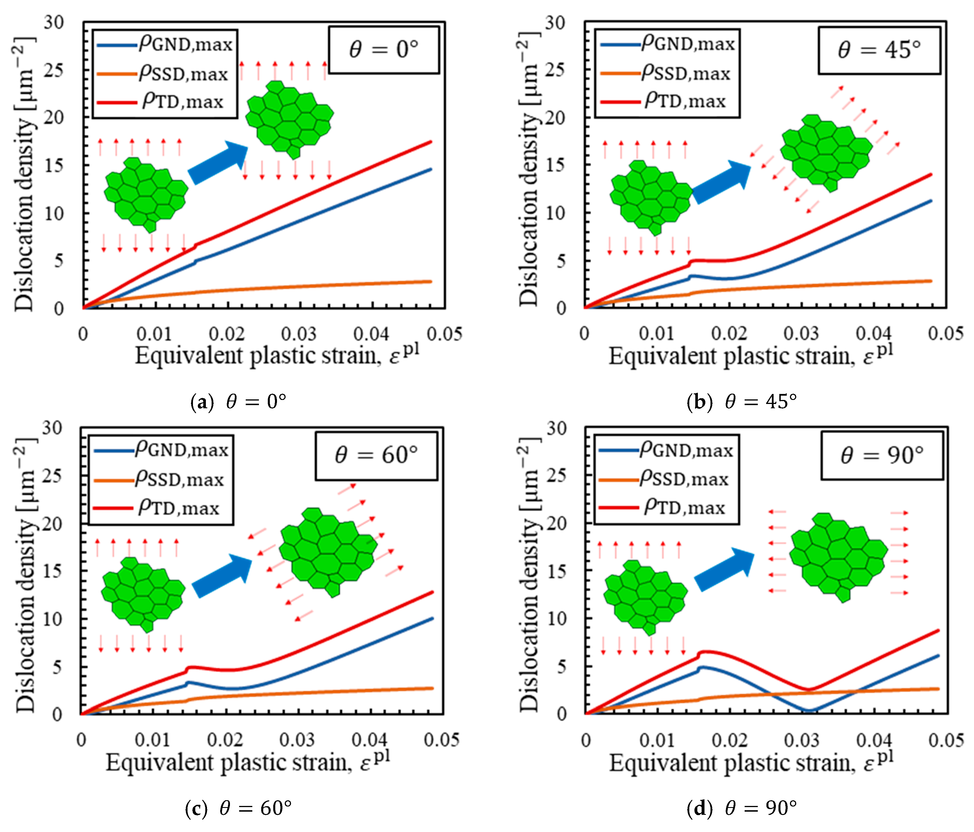
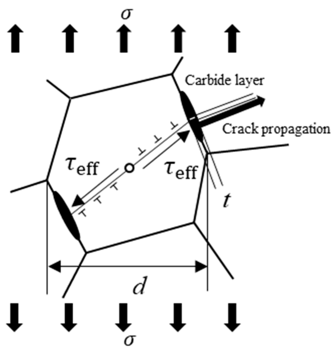
4.2. Analysis of the Crystal Plasticity Model

In this subsection, the strain gradient plasticity (SGP) theory was used based on the crystal plasticity model. First, the theory of SGP is introduced. The SGP theory was proposed in 1970 by Ashby [35], and to date, many studies pertaining to SGP formulation have been carried out [36,37,38,39]. The SGP theory is based on the assumption that not only the plastic strain but also the plastic strain gradient should contribute to the work of deformation in a body. Additionally, one of the advantages of this approach is that the events that occur during plastic deformation at the grain boundary can be explained using the polycrystalline model and SGP theory. The steel material is polycrystalline and has stress and strain gradients in each grain even under macroscopically homogeneous strain conditions. However, in the conventional continuum macroscopic model, the stress and strain cannot be calculated for every grain; only the average value is calculated. To understand the phenomenon of polycrystallinity, it is important to apply a polycrystalline model. Additionally, the computational cost associated with the use of the SGP theory is much lower than that of the conventional crystal plasticity finite element method (CPFEM) because the SGP theory simplifies the average crystal orientation of each grain. Additionally, the SGP theory can calculate the dislocation density expressed by the plastic strain gradient and equivalent plastic strain. As mentioned in Section 1, brittle fracture of steel occurs when a microcrack is generated due to piled-up dislocations in the brittle phase, so it is important to deepen the understanding of dislocation distributions to discuss the embrittlement mechanism. There are two types of dislocations: geometrically necessary dislocations (GNDs) and statistically stored dislocations (SSDs). GNDs depend on the plastic strain gradient, whereas SSDs depend on the equivalent plastic strain. Martínez et al. [40] showed that the densities of these dislocations can be calculated with Equations (14) and (15).

$${\rho }_{\mathrm{GND}}=\overline{r}\frac{{\eta }^{\mathrm{p}}}{b}$$

(14)

$${\rho }_{\mathrm{SSD}}={\left[{\sigma }_{\mathrm{ref}}f\left({\epsilon }^{\mathrm{p}}\right)/\left(M\alpha \mu b\right)\right]}^2$$

(15)

where $b$ is the magnitude of the Burgers vector, $\overline{r}$, $M$ and $\alpha$ are intrinsic material parameters, $\mu$ is the shear modulus, and ${\eta }^{\mathrm{p}}$ is the equivalent plastic strain gradient. Note that ${\eta }^{\mathrm{p}}$ and ${\sigma }_{\mathrm{ref}}f\left({\epsilon }^{\mathrm{p}}\right)$ can be calculated with Equations (16)–(18).

$${\eta }^{\mathrm{p}}=\sqrt{\frac{1}{4}{\displaystyle \sum }_{i,j,k}{\epsilon }_{ij,k}^{\mathrm{p}}{\epsilon }_{ij,k}^{\mathrm{p}}}$$

(16)

$${\epsilon }_{ij,k}^{\mathrm{p}}=\frac{\partial {\epsilon }_{ij}^{\mathrm{p}}}{\partial x_k}$$

(17)

$${\sigma }_{\mathrm{ref}}f\left({\epsilon }^{\mathrm{p}}\right)={\sigma }_{\mathrm{yield}}{\left(\frac{E}{{\sigma }_{\mathrm{yield}}}\right)}^N{\left({\epsilon }^{\mathrm{p}}+{\sigma }_{\mathrm{yield}}/E\right)}^2$$

(18)

where $N$ is the strain hardening coefficient and ${\sigma }_{\mathrm{yield}}$ is the yield stress. Additionally, Gudmundson [39] showed that the principle of virtual work can be calculated with Equation (19).

$$\underset{\mathsf{\Omega }}{\overset{}{{\displaystyle \int }}}\left[{\sigma }_e{}_{ij}\delta {\epsilon }_{ij}+q_{ij}\delta {\epsilon }_{ij}^{\mathrm{p}}+m_{ijk}\delta {\epsilon }_{ij,k}^{\mathrm{p}}\right]dV+\underset{S^{\mathsf{\Gamma }}}{\overset{}{{\displaystyle \int }}}\left[{\check{M}}_{ij}\delta {\widehat{\epsilon }}_{ij}+{\widehat{M}}_{ij}\delta {\check{\epsilon }}_{ij}\right]dS=\underset{S^{\mathrm{ext}}}{\overset{}{{\displaystyle \int }}}\left[{\sigma }_{ij}{n}_j\delta u_i+m_{ijk}{n}_k\delta {\epsilon }_{ij}^p\right]dS$$

(19)

where ${\sigma }_e{}_{ij}$ is the elastic stress, $q_{ij}$ is the plastic stress, $m_{ijk}$ is the moment stress, $M_{ij}$ is the moment traction, ${\widehat{\epsilon }}_{ij}$ is the average strain, and ${\check{\epsilon }}_{ij}$ is the difference in strain between two grains. In Equation (19), the first term on the left side represents the work in the grain, the second term on the left side represents the work in the grain boundary, and the term on the right side represents the work by external force.

In this analysis, a polycrystalline microstructure was simulated so that the average grain diameter was approximately 30$\mathsf{\mu }\mathrm{m}$, and a prestrain test was simulated. It is well known that TMCP steel plates for actual applications have ausformed bainite microstructures, which contain many secondary phases inside prior austenite grains [22]. Kitade et al. [41] carried out a series of sophisticated experiments and reported that the brittle fracture initiation site for this type of steel is located at martensite–austenite (MA) constituents formed at high angle grain boundaries and that there are scarcely high value areas of kernel average misorientation (KAM). The KAM is an index obtained from electron backscatter diffraction (EBSD) analysis corresponding to the dislocation density inside of prior austenite grains just before brittle crack initiation. Through these experimental findings, the authors believe that this assumption of grain size is appropriate.

First, the model was loaded with a 1% prestrain in the vertical direction, and then the fracture test was simulated so that the model was loaded with tensile strain in the direction of $\theta$ rotation. As mentioned above, SGP theory can calculate the individual dislocation densities, ${\rho }_{\mathrm{GND}}$ and ${\rho }_{\mathrm{SSD}}$. The total dislocation density (${\rho }_{\mathrm{TD}}$), which is a sum of ${\rho }_{\mathrm{GND}}$ and ${\rho }_{\mathrm{SSD}}$, was defined as the evaluation value of material damage. Figure 8 shows the history of ${\rho }_{\mathrm{TD},\max }$ for each condition. Here, ${\rho }_{\mathrm{TD},\max }$ is denoted as the value at the center of the element in which ${\rho }_{\mathrm{TD}}$ exhibited the maximum value. Similarly, ${\rho }_{\mathrm{GND},\max }$ and ${\rho }_{\mathrm{SSD},\max }$ are the values of ${\rho }_{\mathrm{GND}}$ and ${\rho }_{\mathrm{SSD}}$ from the element that exhibited ${\rho }_{\mathrm{TD},\max }$. In all cases, the elements that exhibited the maximum ${\rho }_{\mathrm{TD}}$ were always located close to the grain boundary. Additionally, equivalent plastic strain in the horizonal axis denoted the global value and calculated as the average value of all element. As shown in Figure 8, the history of ${\rho }_{\mathrm{TD},\max }$ varies greatly depending on the prestrain direction. When the changes in ${\rho }_{\mathrm{GND},\max }$ and ${\rho }_{\mathrm{SSD},\max }$ are compared, it is clear that ${\rho }_{\mathrm{GND},\max }$ is largely changed for each prestrain direction, whereas ${\rho }_{\mathrm{SSD},\max }$ shows a constant change that is approximately independent of the prestrain direction. This is because ${\rho }_{\mathrm{SSD},\max }$ depends on the equivalent plastic strain, as shown in Equation (15). Focusing on the change in the history of ${\rho }_{\mathrm{GND},\max }$ evolution, ${\rho }_{\mathrm{TD},\max }$ and ${\rho }_{\mathrm{GND},\max }$ continuously increase only when $\theta =0°$, whereas when θ $\ne$ 0°, these values decrease and then increase again. This may reflect the fact that piled-up dislocations move in the opposite direction after load reversal. When $\theta =45$° and 60°, it is understood that load reversal did not occur in the completely opposite direction, but partial load reversal occurred; hence, ${\rho }_{\mathrm{TD},\max }$ slightly decreased just after the beginning of the secondary load. It can be regarded that material damage does not progress while ${\rho }_{\mathrm{TD},\max }$ decreases. Therefore, during some range just after load reversal when $\theta =45°$, $60°$, and $90°$, it is supposed that the damage did not progress. According to Figure 8, the range was the largest in the condition of $\theta =90°$, which can be the reason why the amount of decrease in ${\sigma }_{\mathrm{cut}-\mathrm{off}}$ is quite small in the case of $\theta =90°$, as shown in Figure 7. In this range where the material damage did not progress, the amount of equivalent plastic strain increased, so the equivalent stress increased, as shown in Equation (10). This mechanism made ${\sigma }_{\mathrm{cut}-\mathrm{off}}$ larger at $\theta =90°$.

Based on the abovementioned assumption, a quantitative discussion was carried out. As shown in Figure 9a, the plastic strain required to reach a certain ${\rho }_{\mathrm{TD},\mathrm{cr}}$ is considered. In this analysis, the plastic strain required to reach ${\rho }_{\mathrm{TD},\mathrm{cr}}$, $17.5{ \mathsf{\mu }\mathrm{m}}^{-2}$, after applying the prestrain was denoted as ${\epsilon }_{\mathrm{fract}}^{\mathrm{pl}}\left(\theta \right)$. Material damage progresses continuously in the condition of $\theta =0°$; therefore, ${\epsilon }_{\mathrm{fract}}^{\mathrm{pl}}\left(\theta \right)$ is smallest in the condition of $\theta =0°$. In contrast, the range where the damage did not progress was largest at $\theta =90°$; therefore, ${\epsilon }_{\mathrm{fract}}^{\mathrm{pl}}\left(\theta \right)$ was largest at $\theta =90°$. Brittle fracture occurred in the originating microcrack due to the density of piled-up dislocations; thus, the criterion of the brittle fracture can be simplified as the critical value of ${\rho }_{\mathrm{TD},\max }$. Here, the assumption that brittle fracture occurred when ${\rho }_{\mathrm{TD}}$ reached $17.5{ \mathsf{\mu }\mathrm{m}}^{-2}$ was tentatively made. Based on this assumption, ${\epsilon }_{\mathrm{fract}}^{\mathrm{pl}}\left(\theta \right)$ describes the amount of plastic strain applied after finishing the prestrain until fracture. As mentioned above, because the equivalent stress is determined by the equivalent plastic strain, the increase in ${\epsilon }_{\mathrm{fract}}^{\mathrm{pl}}\left(\theta \right)$ directly corresponds to the increase in ${\sigma }_{\mathrm{cut}-\mathrm{off}}$. Figure 9b shows the relationship between ${\epsilon }_{\mathrm{fract}}^{\mathrm{pl}}\left(\theta \right)$ and dimensionless ${\sigma }_{\mathrm{cut}-\mathrm{off}}$ when 1% prestrain was applied. As shown in Figure 9b, there is a strong correlation between ${\epsilon }_{\mathrm{fract}}^{\mathrm{pl}}\left(\theta \right)$ and ${\sigma }_{\mathrm{cut}-\mathrm{off}}$; hence, ${\sigma }_{\mathrm{cut}-\mathrm{off}}$ increases with increasing ${\epsilon }_{\mathrm{fract}}^{\mathrm{pl}}\left(\theta \right)$. Furthermore, when the amount of prestrain increased, ${\rho }_{\mathrm{TD},\max }$ increased and ${\epsilon }_{\mathrm{fract}}^{\mathrm{pl}}\left(\theta \right)$ decreased. As a result, ${\sigma }_{\mathrm{cut}-\mathrm{off}}$ is considered to decrease, and this result matches Figure 7.

Thus, it is understood that the change in ${\sigma }_{\mathrm{cut}-\mathrm{off}}$ can be explained by the change in ${\epsilon }_{\mathrm{fract}}^{\mathrm{pl}}\left(\theta \right)$, i.e., the way material damage progresses due to piled-up dislocations. In the next section, based on these mechanisms, a formulation is presented for the change in critical stress after prestrain application.

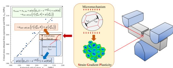
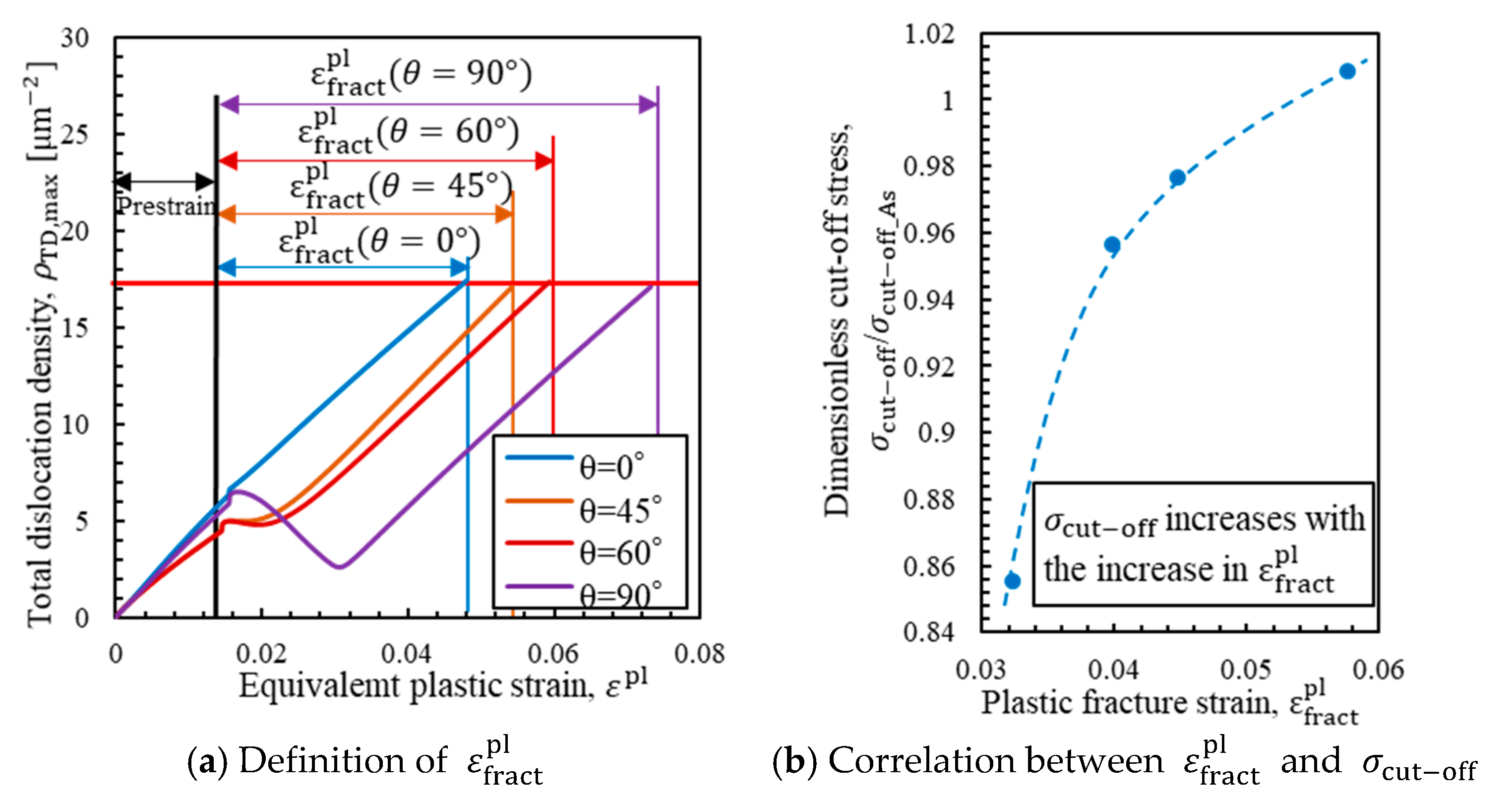
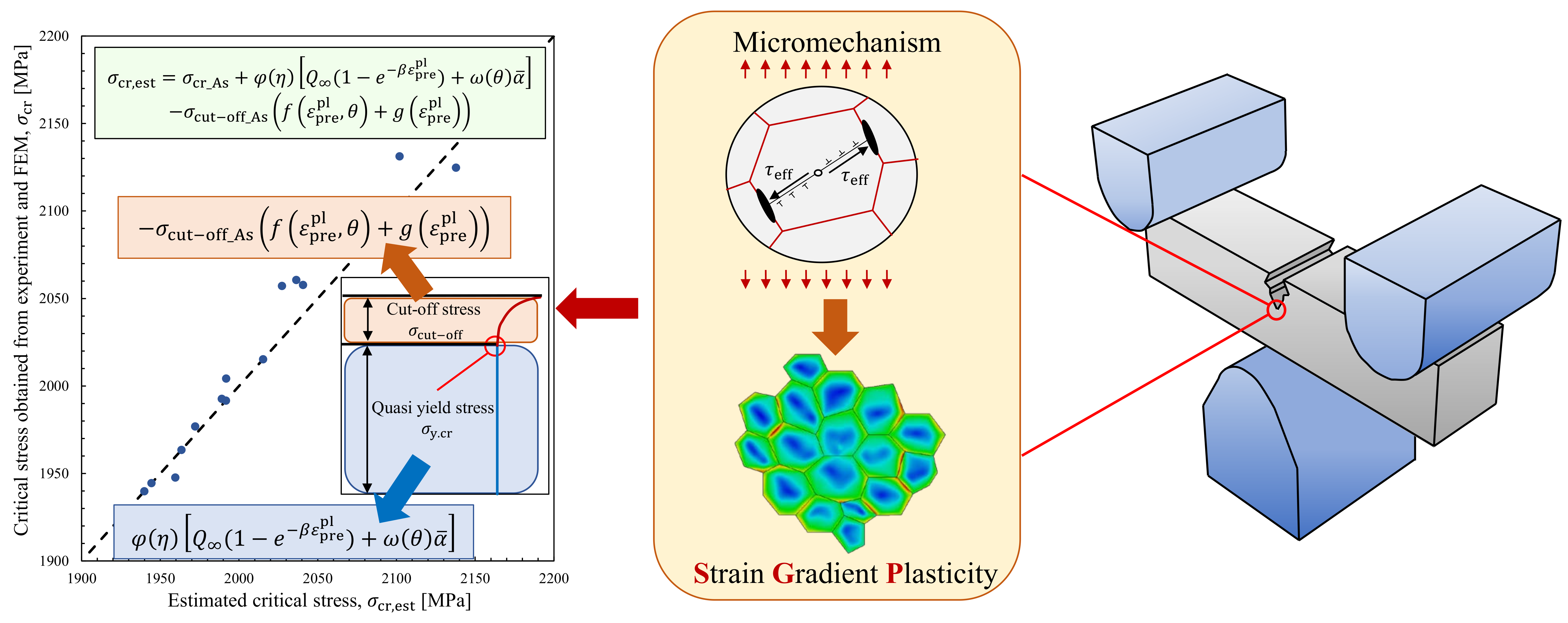
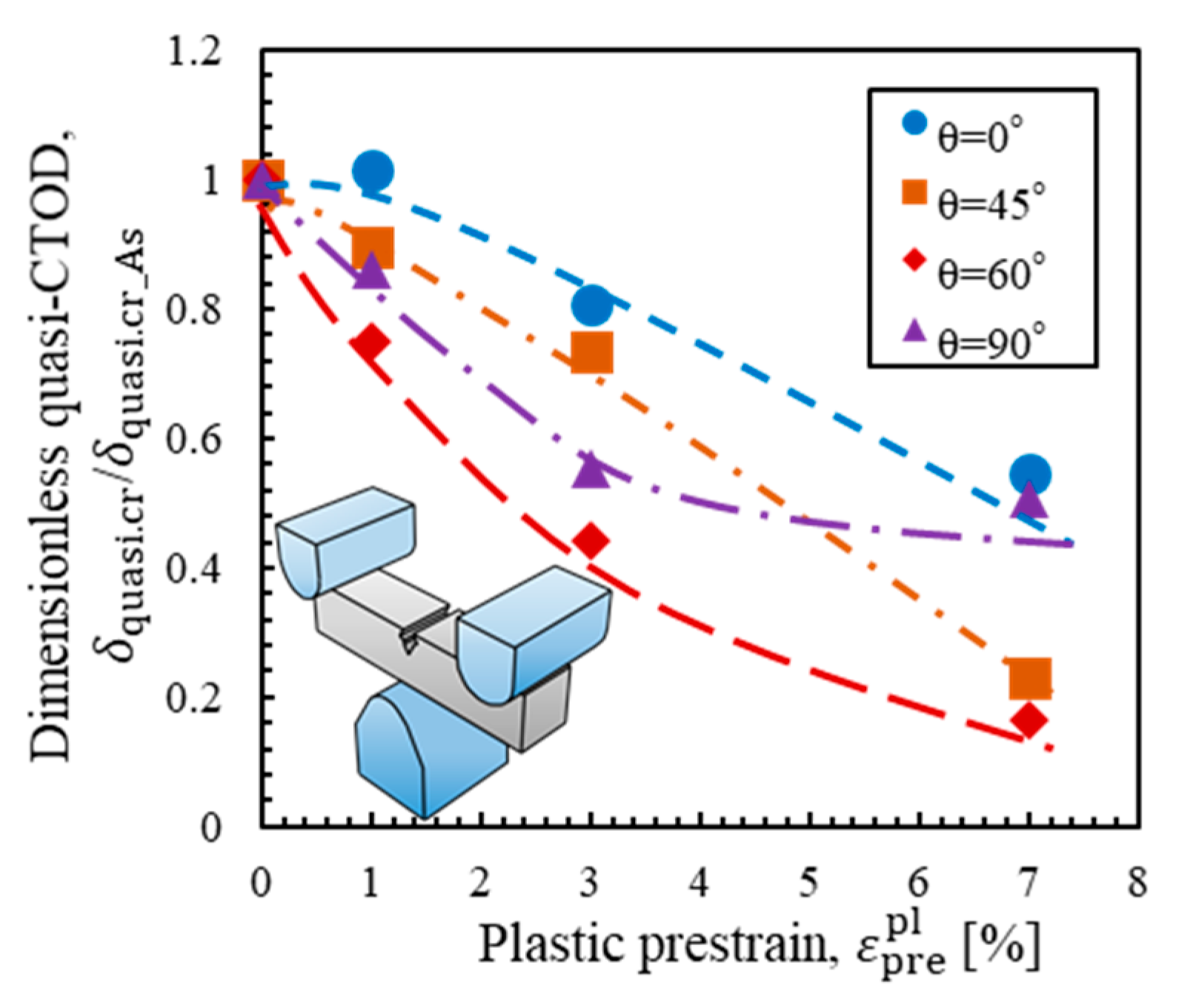
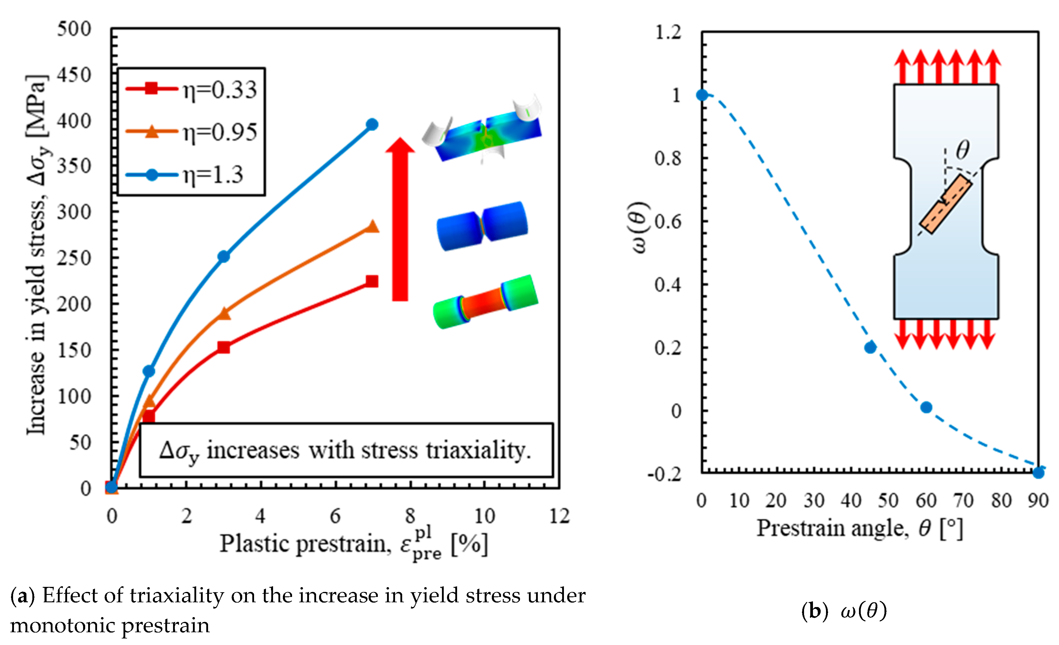
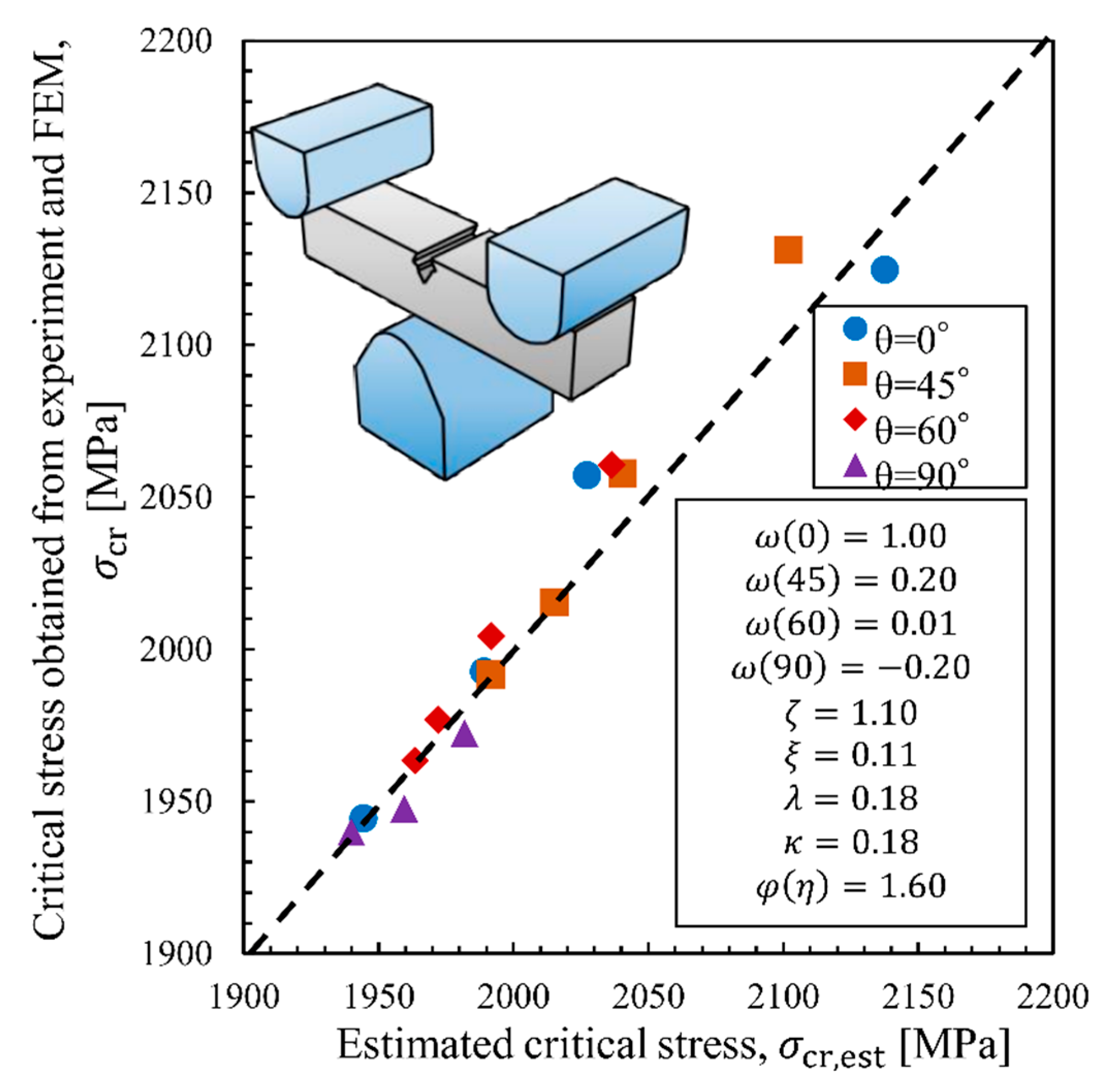
5. Formulation of Critical Stress Change from Various Prestrains

In the previous section, the change in critical stress can be expressed by the increase in yield stress and the decrease in ${\sigma }_{\mathrm{cut}-\mathrm{off}}$. Based on this theory, the formulation of critical stress is carried out. First, the general form for the elastic component of the critical stress in the fracture test is proposed in Equation (20).

$${\sigma }_{\mathrm{el}}={\sigma }_{\mathrm{el}\_\mathrm{As}}+\phi \left(\eta \right)\left[Q_{\infty }\left(1-e^{-\beta {\epsilon }_{\mathrm{pre}}^{\mathrm{pl}}}\right)+\omega \left(\theta \right)\overline{\alpha }\right]$$

(20)

where ${\sigma }_{\mathrm{el}\_\mathrm{As}}$ is the elastic component of critical stress without prestraining, $\phi \left(\eta \right)$ is a function of $\eta$ that is set equal to one for uniaxial stress conditions, ${\epsilon }_{\mathrm{pre}}^{\mathrm{pl}}$ is the plastic prestrain, $\omega \left(\theta \right)$ is a function of $\theta$, and $Q_{\infty }\left(1-e^{-\beta {\epsilon }_{\mathrm{pre}}^{\mathrm{pl}}}\right)+\omega \left(\theta \right)\overline{\alpha }$ represents the combined hardening rule. As shown in Figure 10a, the amount of increase in yield stress is larger with high stress triaxiality. Therefore, because the sharp-notched bending specimen used in this study has high triaxiality, the amount of increase in yield stress increases. Here, it was assumed that the increase in yield stress rises linearly with respect to triaxiality, and $\phi \left(\eta \right)$ was set to 1.60 for this specimen in this paper. It should be noted, however, that in order to determine this value accurately, it must be determined experimentally using specimens with different multiaxiality. Additionally, $\omega \left(\theta \right)$ is the function that expresses the degree of the Bauschinger effect, which is a function of the period. As shown in Figure 10b, $\omega \left(\theta \right)$ is largest at $\theta =0°$ and smallest at $\theta =90°$. In this study, $\omega \left(\theta \right)$ was set to 1.0 at $\theta =0°$ and −0.20 at $\theta =90°$.

Hereafter, ${\sigma }_{\mathrm{cut}-\mathrm{off}}$ is discussed. As mentioned above, ${\sigma }_{\mathrm{cut}-\mathrm{off}}$ is considered to be greatly affected by the difference in piled-up dislocations. When load reversal occurs, dislocations pile up in the opposite direction, and there is some range where material damage does not progress, which restrains the decrease in ${\sigma }_{\mathrm{cut}-\mathrm{off}}$. However, when load reversal occurs, dislocations not only pile up like GNDs but are also simply stored like SSDs. Therefore, the effect of material damage due to both piled-up dislocations and stored dislocations should be considered.

First, the effect of piled-up dislocations is considered. This effect strongly depends on the prestrain direction. Here, the damage due to piled-up dislocations is defined in Equation (21).

$$f\left({\epsilon }_{\mathrm{pre}}^{\mathrm{pl}}, \theta \right)=\lambda \omega \left(\theta \right)\left\{1-\exp \left(-\zeta {\epsilon }_{\mathrm{pre}}^{\mathrm{pl}}\right)\right\}$$

(21)

Equation (21) is a monotonically increasing function with respect to ${\epsilon }_{\mathrm{pre}}^{\mathrm{pl}}$ and expresses the material damage due to piled-up dislocations. Additionally, this function is designed to converge to $\lambda \omega \left(\theta \right)$ in the case of a sufficiently high value of ${\epsilon }_{\mathrm{pre}}^{\mathrm{pl}}$, which corresponds to the phenomenon that the parameter of brittle fracture toughness, such as the critical CTOD, converges to a certain low value even if there is a sufficiently high amount of prestrain. $\omega \left(\theta \right)$ is the same function used in Equation (20), which corresponds to how dislocations are moved in the opposite direction. The range where material damage does not progress increases with increasing $\theta$. Therefore, Equation (21) shows that material damage decreases with a high value of $\theta$.

Hereafter, the effect of stored dislocations is considered. This damage is considered to be independent of the prestrain direction and depends only on the amount of prestrain because the stored dislocations are considered to increase monotonically with respect to the equivalent plastic strain, whereas piled-up dislocations strongly depend on the prestrain direction. The damage due to stored dislocations is defined in Equation (22).

$$g\left({\epsilon }_{\mathrm{pre}}^{\mathrm{pl}}\right)=\kappa \left\{1-\exp \left(-\xi {\epsilon }_{\mathrm{pre}}^{\mathrm{pl}}\right)\right\}$$

(22)

Equation (22) is a monotonically increasing function with respect to ${\epsilon }_{\mathrm{pre}}^{\mathrm{pl}}$ and converges to $\kappa$ in the case of a sufficiently high value of ${\epsilon }_{\mathrm{pre}}^{\mathrm{pl}}$, similar to Equation (21). Combining Equation (21) and Equation (22), the decrease in ${\sigma }_{\mathrm{cut}-\mathrm{off}}$ is defined in Equation (23).

$$\mathsf{\Delta }{\sigma }_{\mathrm{cut}-\mathrm{off}}=-{\sigma }_{\mathrm{cut}-\mathrm{off}\_\mathrm{As}}\left[\lambda \omega \left(\theta \right)\left\{1-\exp \left(-\zeta {\epsilon }_{\mathrm{pre}}^{\mathrm{pl}}\right)\right\}+\kappa \left\{1-\exp \left(-\xi {\epsilon }_{\mathrm{pre}}^{\mathrm{pl}}\right)\right\}\right]$$

(23)

Finally, the change in critical stress is calculated by combining Equation (20) and Equation (23). The critical stress after prestraining can be determined with Equation (24).

$${\sigma }_{\mathrm{cr},\mathrm{est}}={\sigma }_{\mathrm{cr}\_\mathrm{As}}+\phi \left(\eta \right)\left[Q_{\infty }\left(1-e^{-\beta {\epsilon }_{\mathrm{pre}}^{\mathrm{pl}}}\right)+\omega \left(\theta \right)\overline{\alpha }\right]-{\sigma }_{\mathrm{cut}-\mathrm{off}\_\mathrm{As}}\left(f\left({\epsilon }_{\mathrm{pre}}^{\mathrm{pl}}, \theta \right)+g\left({\epsilon }_{\mathrm{pre}}^{\mathrm{pl}}\right)\right)$$

(24)

Figure 11 shows a comparison between the critical stress calculated from Equation (24) and that calculated from FEM analysis. As shown in Figure 11, the critical stress can be estimated with high precision using Equation (24). The parameters shown in Figure 11 were determined based on SGP theory. Additionally, except $\phi \left(\eta \right)$, these are considered to depend on microstructure, so these values can be used in different test specimen if the same material is used. Thus, the critical stress can be estimated for specimens with various levels of prestrain in different directions subjected to fracture tests with different levels of triaxiality.

6. Conclusions

In this study, the effect of the prestraining direction and its amount on the critical stress of brittle fracture was investigated. Additionally, a new formula for accurately estimating critical stress was proposed based on the micromechanism obtained from the SGP theory, from which the following findings were obtained:

• It was verified that the critical stress increased due to the application of prestrain at any angle, and the ratio of this increase varied strongly with respect to the prestrain direction. This finding is different from Griffith’s equation or Smith’s model, in which the critical stress is determined only by the length of the microcrack or the thickness of the carbide particles and the remote stress.
• It was shown that the increase in critical stress can be separately explained by the increase in yield stress and the decrease in ${\sigma }_{\mathrm{cut}-\mathrm{off}}$. Additionally, the decrease in ${\sigma }_{\mathrm{cut}-\mathrm{off}}$ represented the effect of embrittlement and strongly depended on the way dislocations were piled up. Using analysis based on the SGP theory, the change in ${\sigma }_{\mathrm{cut}-\mathrm{off}}$ was shown to be affected by piled-up dislocations that moved in the opposite direction during load reversal.
• The change in critical stress can be formulated based on the micromechanisms. The critical stress was calculated by the triaxiality of the fracture test and the amount and direction of prestrain. It was shown that critical stress can be estimated with high accuracy by giving appropriate parameters.

In this study, many new findings on the critical stress that have not been previously discussed were presented. However, there are still many problems to be solved in this study. First, the present prestrain was introduced in a uniaxial state, whereas the strain in an actual structure is always loaded in a multiaxial state. In addition, in the critical stress formulation, there are many material-dependent parameters, and it is desirable to construct a universal model that can be applied to any material. Additionally, this model has been developed on the assumption that dislocations dominate the damage, but the mechanism may differ in a material in which the brittle crack initiation position is located at large and hard particles, such as MA or cementite, inside of grains. The effect of the microstructure on the critical stress after prestrain should be investigated in future studies.

References

1. Griffith, A.A. The phenomena of rupture and flow in solid. Philos. Trans. Ser. A 1920, 221, 163–198. [Google Scholar]
2. Inglis, C.E. Stresses in a Plate Due to the Presence of Cracks and Sharp Corners. Trans. Inst. Nav. Archit. 1913, 55, 219–241. [Google Scholar]
3. Stroh, A. A theory of the fracture of metals. Adv. Phys. 1957, 6, 418–465. [Google Scholar] [CrossRef]
4. Smith, E. The nucleation and growth of cleavage microcracks in mild steel. Phys. Basis Yield Fract. Conf. Proc. 1966, 1966, 36–46. [Google Scholar]
5. Hall, E.O. The deformation and aging of mild steel. Proc. Phys. Soc. Sect. B 1951, 64, 747–753. [Google Scholar] [CrossRef]
6. Petch, N.J. The Cleavage Strength of Polycrystals. J. Iron Steel Inst. 1953, 174, 25–28. [Google Scholar]
7. Cottrell, A.H. Theory of brittle fracture in steel and similar metals. Trans. Metall. Soc. AIME 1959, 212, 192–201. [Google Scholar]
8. Epstein, B. Statistical approach to brittle fracture. J. Appl. Phys. 1948, 19, 140–147. [Google Scholar] [CrossRef]
9. Beremin, F.M. A local criterion for cleavage fracture of a nuclear pressure vessel steel. Metall. Trans. A 1983, 14, 2277–2287. [Google Scholar] [CrossRef]
10. Bordet, S.R.; Karstensen, A.D.; Knowles, D.M.; Wiesner, C.S. A new statistical local criterion for cleavage fracture in steel. Part I: Model presentation. Eng. Fract. Mech. 2005, 72, 435–452. [Google Scholar] [CrossRef]
11. Bordet, S.; Karstensen, A.; Knowles, D.; Wiesner, C. A new statistical local criterion for cleavage fracture in steel. Part II: Application to an offshore structural steel. Eng. Fract. Mech. 2005, 72, 453–474. [Google Scholar] [CrossRef]
12. Lei, W.-S. A cumulative failure probability model for cleavage fracture in ferritic steels. Mech. Mater. 2016, 93, 184–198. [Google Scholar]
13. Lei, W.-S. A discussion of “An engineering methodology for constraint corrections of elastic–plastic fracture toughness—Part II: Effects of specimen geometry and plastic strain on cleavage fracture predictions” by C. Ruggieri, R.G. Savioli, R.H. Dodds [Eng. Fract. Mech. 146 (2015) 185–209]. Eng. Fract. Mech. 2017, 178, 527–534. [Google Scholar] [CrossRef]
14. McMahon, C.; Cohen, M. Initiation of cleavage in polycrystalline iron. Acta Met. 1965, 13, 591–604. [Google Scholar] [CrossRef]
15. Gurland, J. Observations on the fracture of cementite particles in a spheroidized 1.05% c steel deformed at room temperature. Acta Met. 1972, 20, 735–741. [Google Scholar]
16. Sukedai, E.; Hid, M. Effect of Tensile Pestrain on Ductile-Brittle Transition Temperture of Low Carbon Steel. Mater. Sci. Monogr. 1982, 15, 112–118. [Google Scholar]
17. Miki, C.; Sasaki, E.; Kyuba, H.; Takenoi, I. Deterioration of Fracture Toughness of Steel by Effect of Tensile and Compressive Prestrain. J. JSCE 2000, 640, 165–175. [Google Scholar]
18. Kosuge, H.; Kawabata, T.; Okita, T.; Murayama, H.; Takagi, S. Establishment of damage estimation rules for brittle fracture after cyclic plastic prestrain in steel. Mater. Des. 2020, 185, 108222. [Google Scholar] [CrossRef]
19. Yoshinari, H.; Enami, K.; Koseki, T.; Shimanuki, H.; Aihara, S. Ductile and brittle fracture initiation behavior for compressively prestrained steel. J. Soc. Nav. Arch. Jpn. 2001, 2001, 559–567. [Google Scholar] [CrossRef]
20. Bordet, S.R.; Tanguy, B.; Bugat, S.; Moinereau, D.; Pineau, A. Cleavage Fracture Micromechanisms Related to WPS Effect in RPV Steel. Fract. Nano Eng. Mater. Struct. 2008, 16, 835–836. [Google Scholar]
21. Tagawa, T.; Itoh, A.; Miyata, T. Ouantitative prediction of embrittlement due to pre-strain for low carbon steels. Q. J. Jpn. Weld. Soc. 1996, 2, 429–434. [Google Scholar] [CrossRef]
22. Nishioka, K.; Ichikawa, K. Progress in thermomechanical control of steel plates and their commercialization. Sci. Technol. Adv. Mater. 2012, 13, 023001. [Google Scholar] [CrossRef] [PubMed]
23. International Organization for Standardization. Petroleum and Natural Gas Industries—Steel Pipe for Pipeline Transportation Systems; ISO 3183:2019; ISO: Geneva, Switzerland, 2019. [Google Scholar]
24. The American Petroleum Institute (API). Steel Plates Produced by Thermo Mechanically Controlled Processing for Offshore Structures. In API Specification 2W, 6th ed.; API: Washington, DC, USA, 2019. [Google Scholar]
25. ASTM International. Standard Specification for Steel Plates for Pressure Vessels, Produced by Thermo-Mechanical Control Process (TMCP); ASTM A841/A841M-17; ASTM International: West Conshohocken, PA, USA, 2017. [Google Scholar]
26. International Association of Classification Societies. Normal and Higher Strength Hull Structural Steels; IACS W11, Rev.9; IACS: London, UK, 2017. [Google Scholar]
27. The Japanese Iron and Steel Federation (JISF). TMCP Steel for Building (TMCP325, TMCP355); MDCR 0016-2016; JISF: Tokyo, Japan, 2016. [Google Scholar]
28. The Japanese Iron and Steel Federation. Rolled Steel with 500N/mm2 Yield Strangth and 700N/mm2 Yield Strength for Welded Structure; MDCR 0014-2004; JISF: Tokyo, Japan, 2005. [Google Scholar]
29. International Organization for Standardization. Metallic Materials—Unified Method of Test for the Determination of Quasistatic Fracture Toughness; ISO12135:2016; ISO: Geneva, Switzerland, 2016. [Google Scholar]
30. Kawabata, T.; Tagawa, T.; Sakimoto, T.; Kayamori, Y.; Ohata, M.; Yamashita, Y.; Tamura, E.-I.; Yoshinari, H.; Aihara, S.; Minami, F.; et al. Proposal for a new CTOD calculation formula. Eng. Fract. Mech. 2016, 159, 16–34. [Google Scholar] [CrossRef]
31. International Organization for Standardization. Metallic Materials—Method of Test for the Determination of Quasistatic Fracture Toughness of Welds; ISO15653:2018; ISO: Geneva, Switzerland, 2018. [Google Scholar]
32. Chaboche, J.L. Constitutive equations for cyclic plasticity and cyclic viscoplasticity. Int. J. Plast. 1989, 5, 247–302. [Google Scholar] [CrossRef]
33. Lemaitre, J.; Chaboche, J.L. Mechanics of Solid Materials; Cambridge University Press: Cambridge, UK, 1994; 584p, ISBN 0521477581/9780521477581. [Google Scholar]
34. Abaqus, version 2018; Dassault Systèmes®: Vélizy-Villacoublay, France, 2018.
35. Ashby, M.F. The deformation of plastically non-homogeneous materials. Philos. Mag. 1970, 21, 399–424. [Google Scholar] [CrossRef]
36. Fleck, N.; Hutchinson, J. A phenomenological theory for strain gradient effects in plasticity. J. Mech. Phys. Solids 1993, 41, 1825–1857. [Google Scholar] [CrossRef]
37. Fleck, N.; Muller, G.; Ashby, M.; Hutchinson, J. Strain gradient plasticity: Theory and experiment. Acta Met. Mater. 1994, 42, 475–487. [Google Scholar] [CrossRef]
38. Fleck, N.A.; Hutchinson, J.W. A reformulation of strain gradient plasticity. J. Mech. Phys. Solids 2001, 49, 2245–2271. [Google Scholar] [CrossRef] [Green Version]
39. Gudmundson, P. A unified treatment of strain gradient plasticity. J. Mech. Phys. Solids 2004, 52, 1379–1406. [Google Scholar] [CrossRef]
40. Martínez-Pañeda, E.; Betegón, C. Modeling damage and fracture within strain-gradient plasticity. Int. J. Solids Struct. 2015, 59, 208–215. [Google Scholar] [CrossRef]
41. Kitade, A.; Kawabata, T.; Kimura, S.; Takatani, H.; Kagehira, K.; Mitsuzumi, T. Clarification of micromechanism on Brittle Fracture Initiation Condition of TMCP Steel with MA as the trigger point. Procedia Struct. Integr. 2018, 13, 1845–1854. [Google Scholar] [CrossRef]
Figure 1. Brittle fracture micromechanism.
Crystals 10 00867 g001
Figure 2. Schematic illustration of the experiment and configuration of the tensile and fracture test specimens. TMCP: thermomechanical control process. (a) Outline of the experiment, (b) Tensile specimen, (c) Fracture test specimen.
Crystals 10 00867 g002
Figure 3. True stress-true strain curves before/after prestraining. (a) θ = 0 ° , (b) θ = 45 ° , (c) θ = 60 ° , (d) θ = 90 ° .
Crystals 10 00867 g003
Figure 4. Toughness degradation in critical CTOD due to prestrain in different directions.
Crystals 10 00867 g004
Figure 5. Change in the critical stress due to prestrain in different directions.
Crystals 10 00867 g005
Figure 6. Change in quasi-yield stress due to prestrain in different directions. (a) Definition of σ y , cr , (b) Change in the dimensionless quasi-yield stress.
Crystals 10 00867 g006
Figure 7. Change in the dimensionless cut-off stress due to prestrain in different directions.
Crystals 10 00867 g007
Figure 8. Change in peak dislocation density for each prestrain condition. (a) θ = 0 ° , (b) θ = 45 ° , (c) θ = 60 ° , (d) θ = 90 ° .
Crystals 10 00867 g008
Figure 9. Mechanism of change in σ cut off during loading with different prestrain directions. (a) Definition of ε fract pl , (b) Correlation between ε fract pl and σ cut off .
Crystals 10 00867 g009
Figure 10. Introduction of coefficients of the proposed elastic component. (a) Effect of triaxiality on the increase in yield stress under monotonic prestrain, (b) ω ( θ ) .
Crystals 10 00867 g010
Figure 11. Accuracy of the proposed formula established to estimate critical stress.
Crystals 10 00867 g011