Characteristics of Water and Urea–Water Solution Sprays


Abstract
:1. Introduction
2. Results and Discussion
2.1. Experimental Study
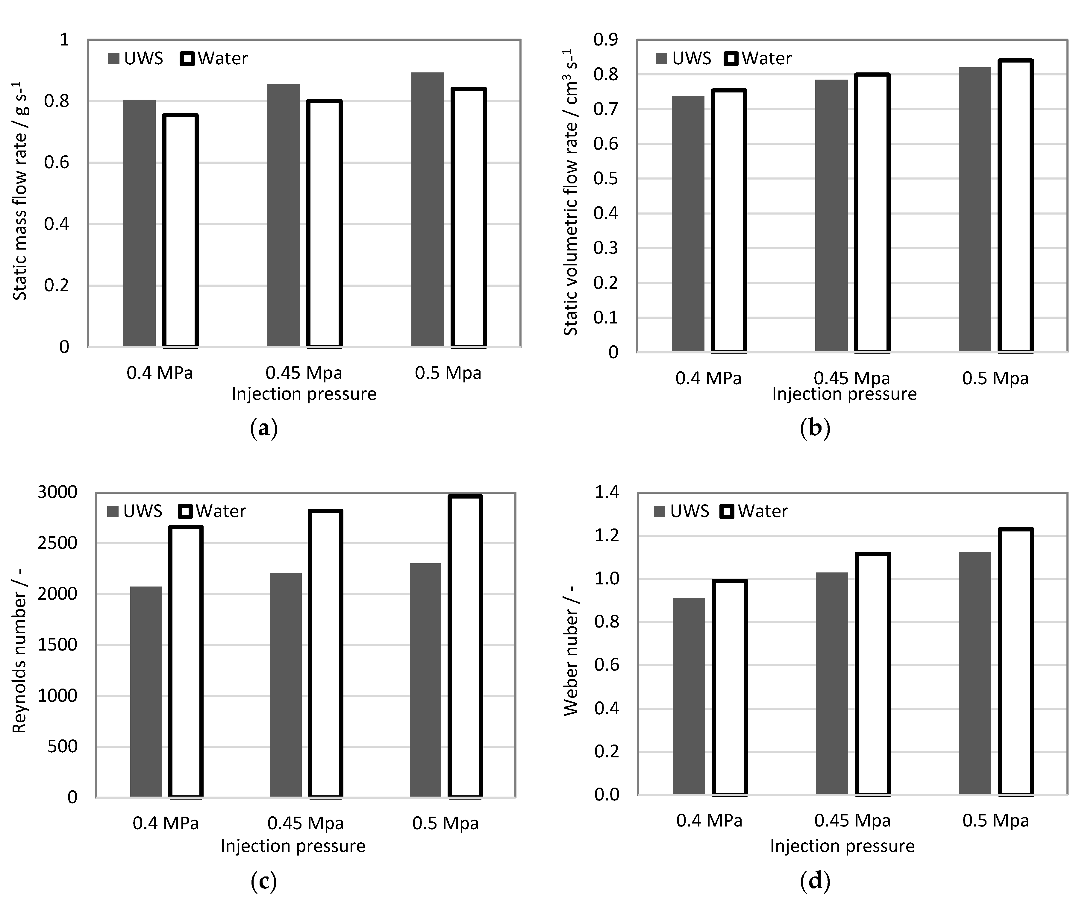
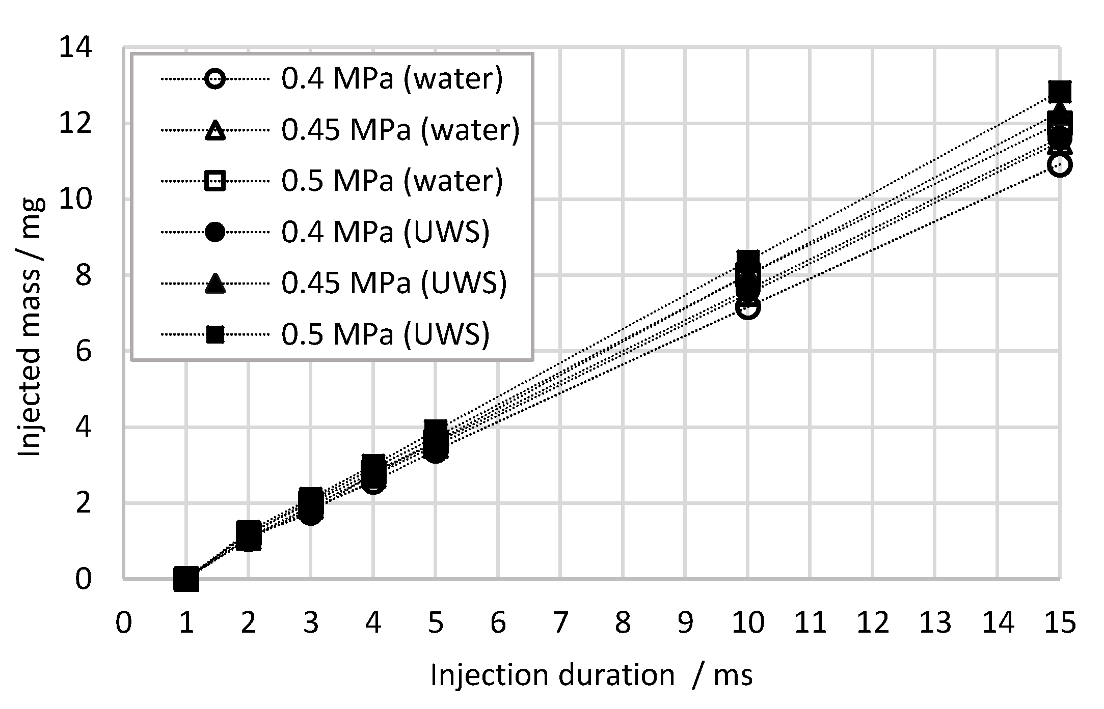
2.1.1. Flow Characteristics
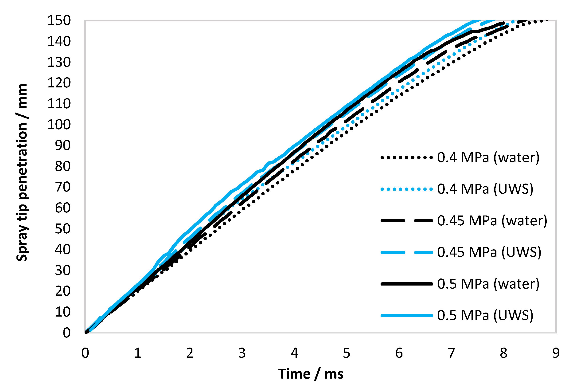
2.1.2. Spray Tip Penetration
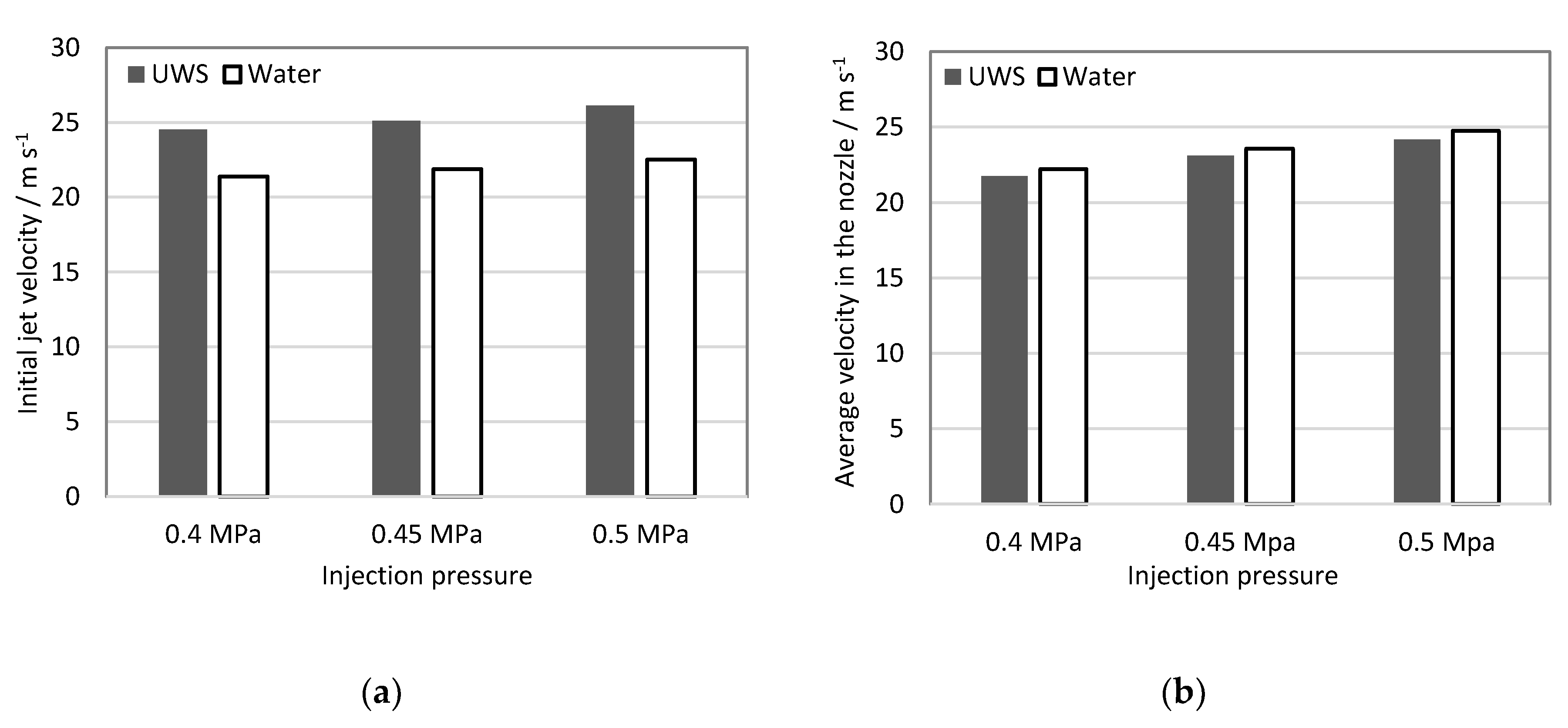
2.1.3. Initial Jet Velocity
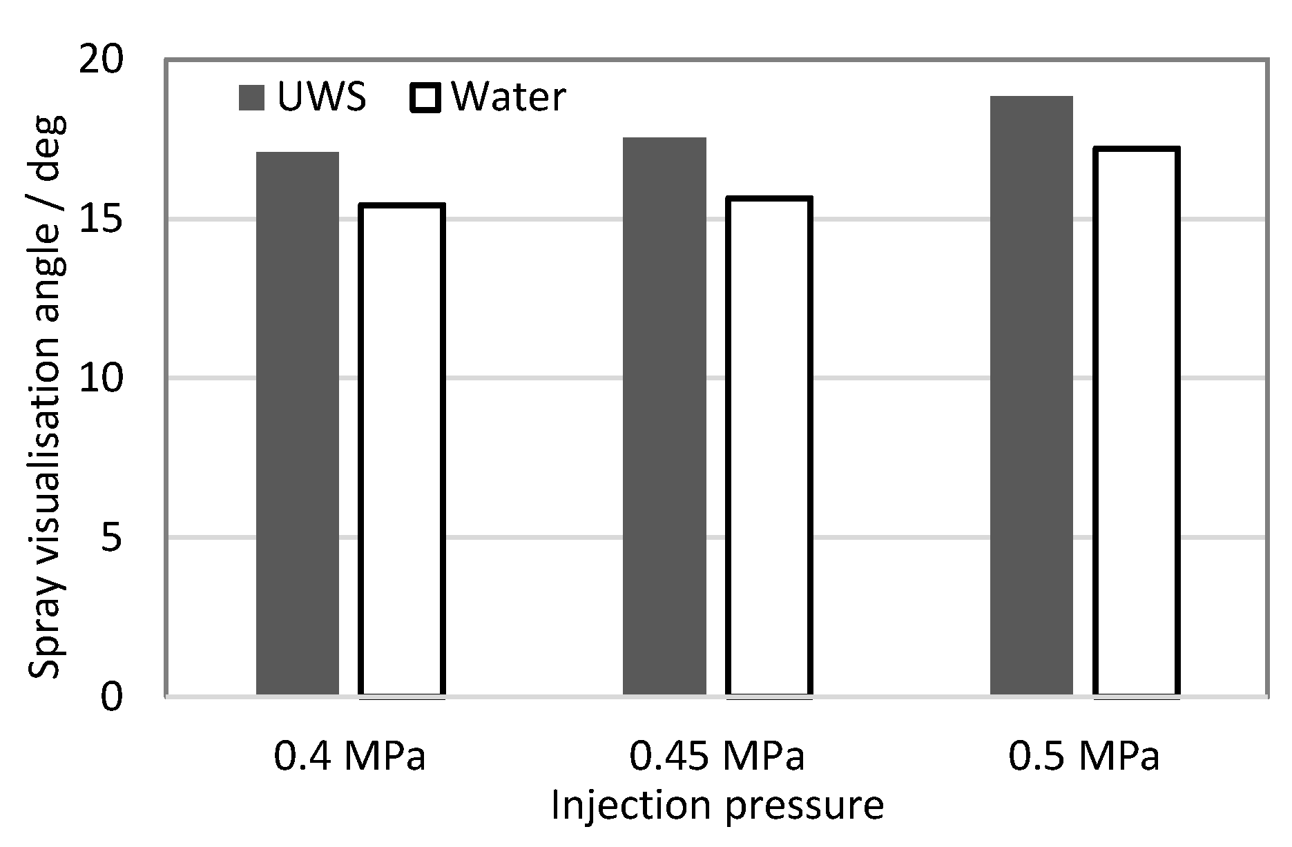
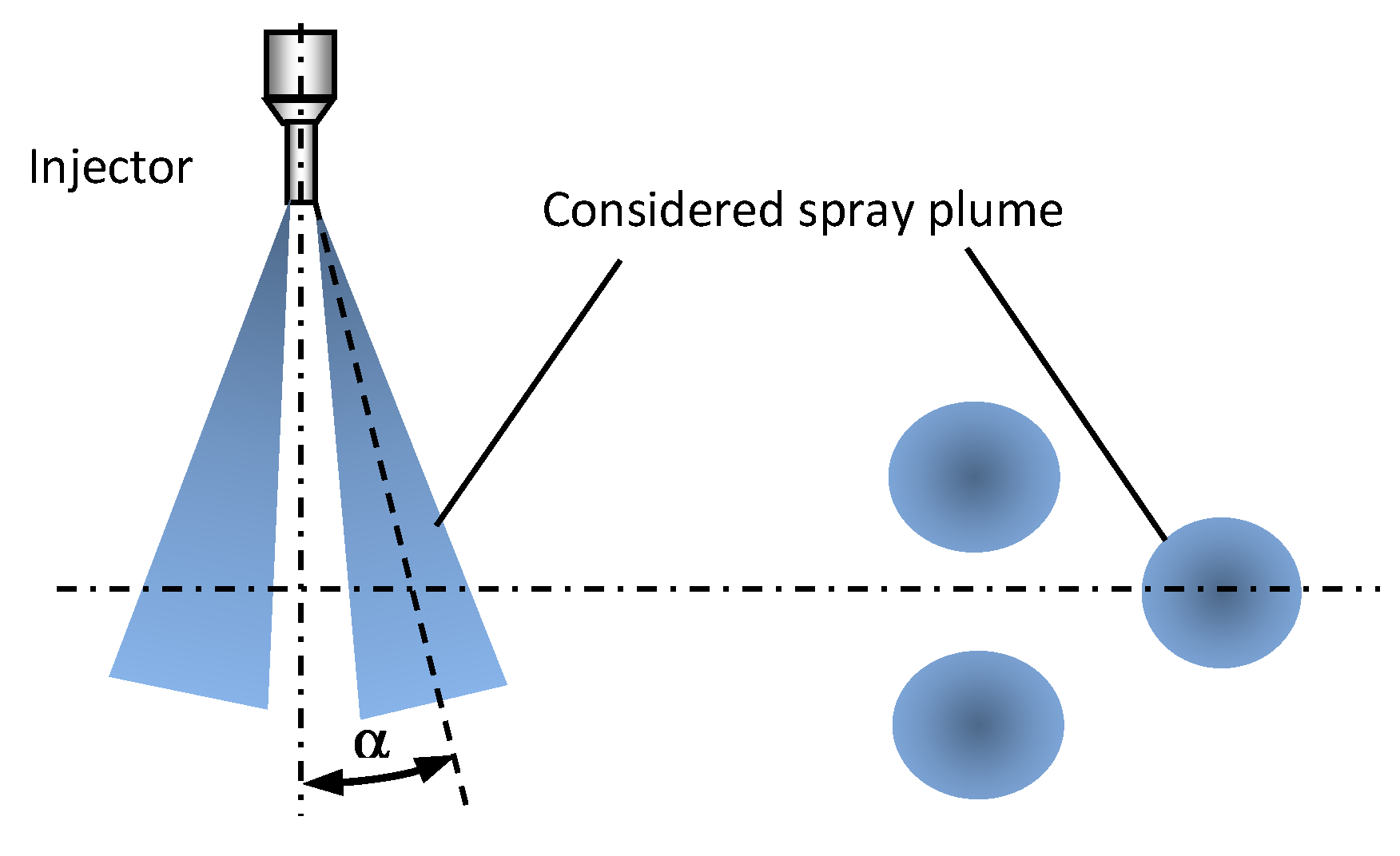
2.1.4. Spray Visualization Angle
2.1.5. Jet Inclination Angle
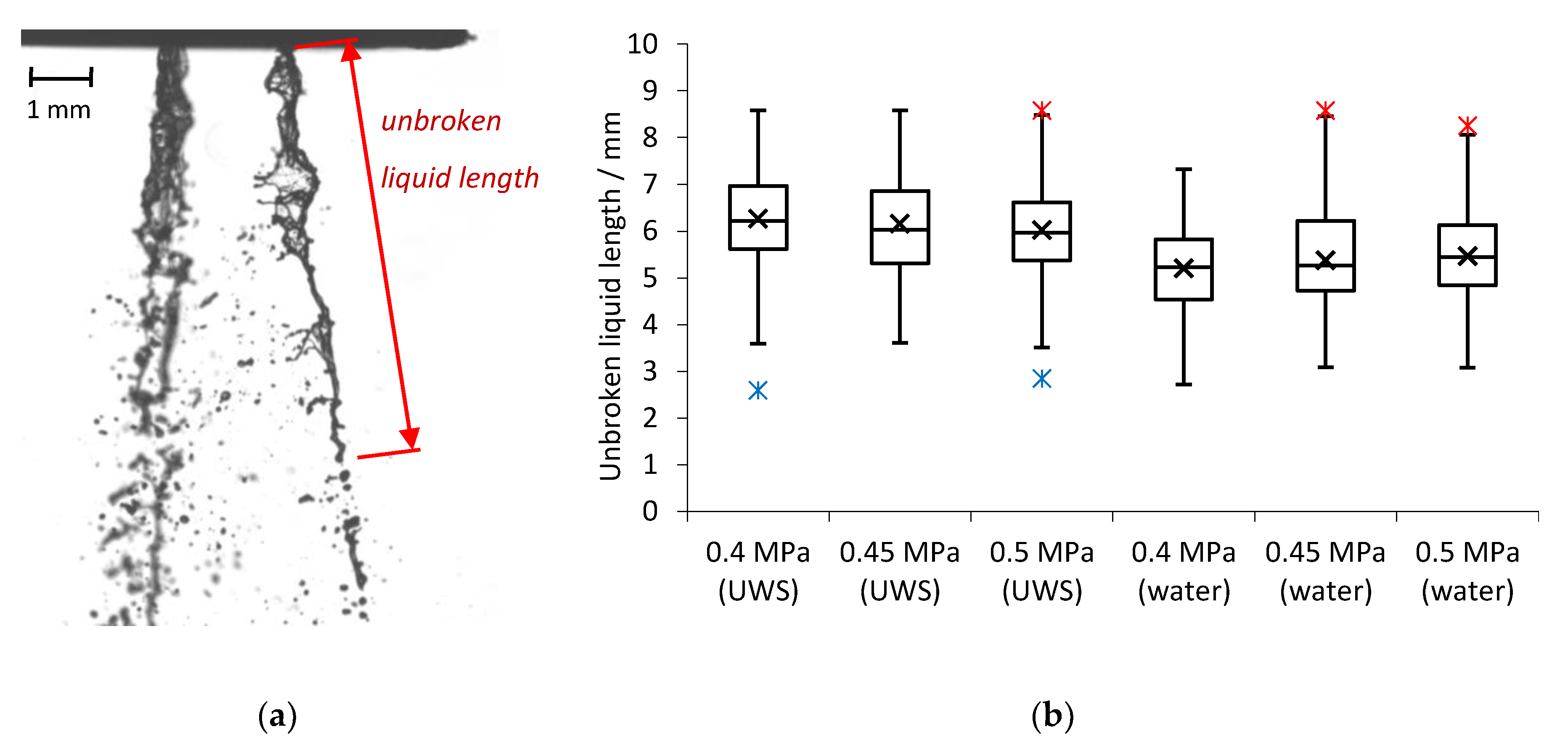
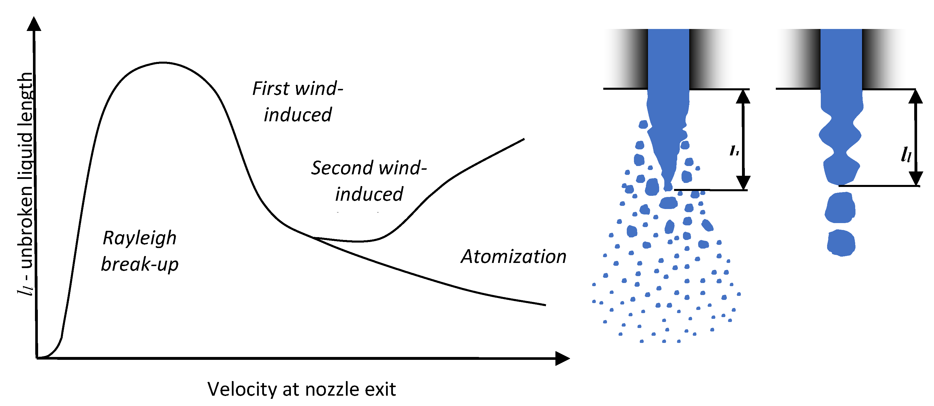
2.1.6. Unbroken Liquid Length
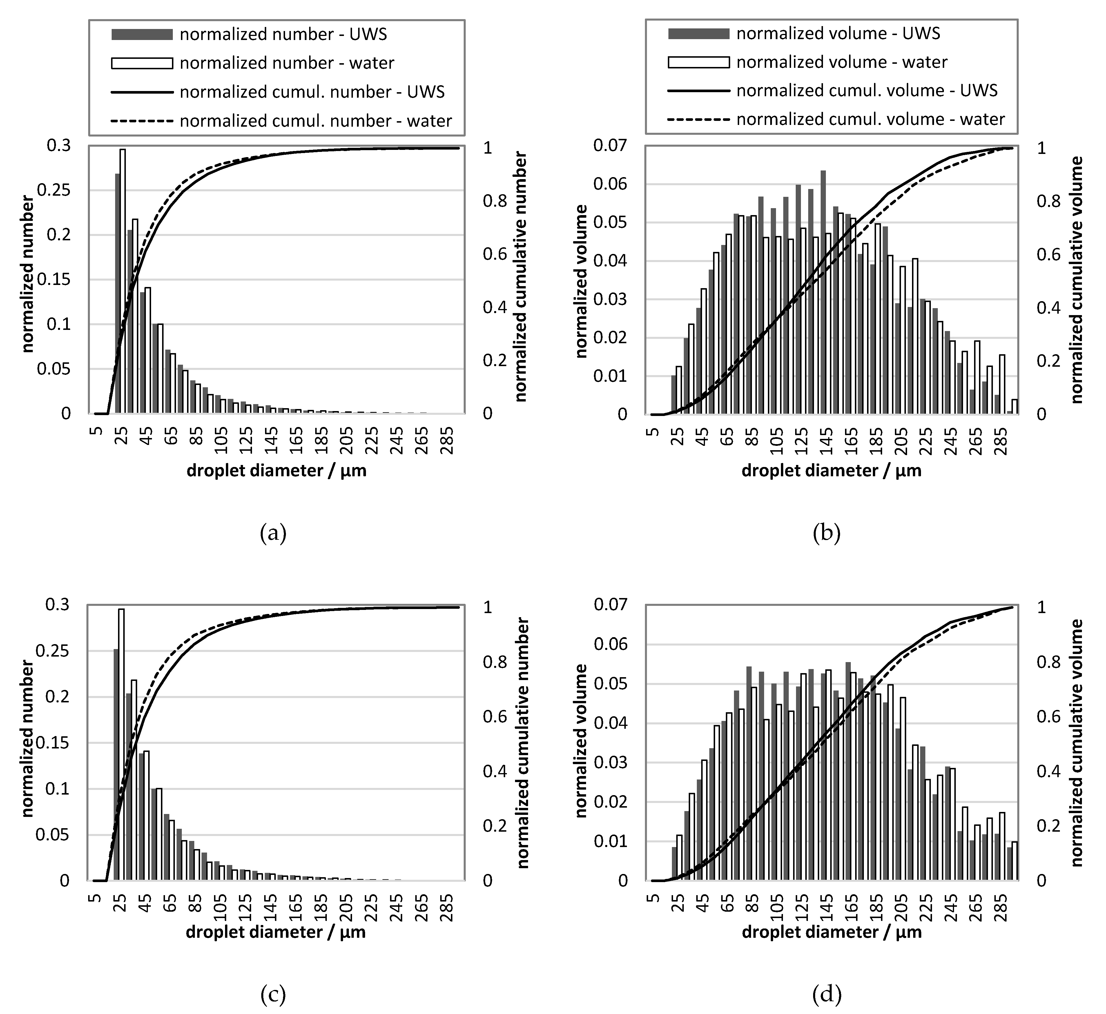
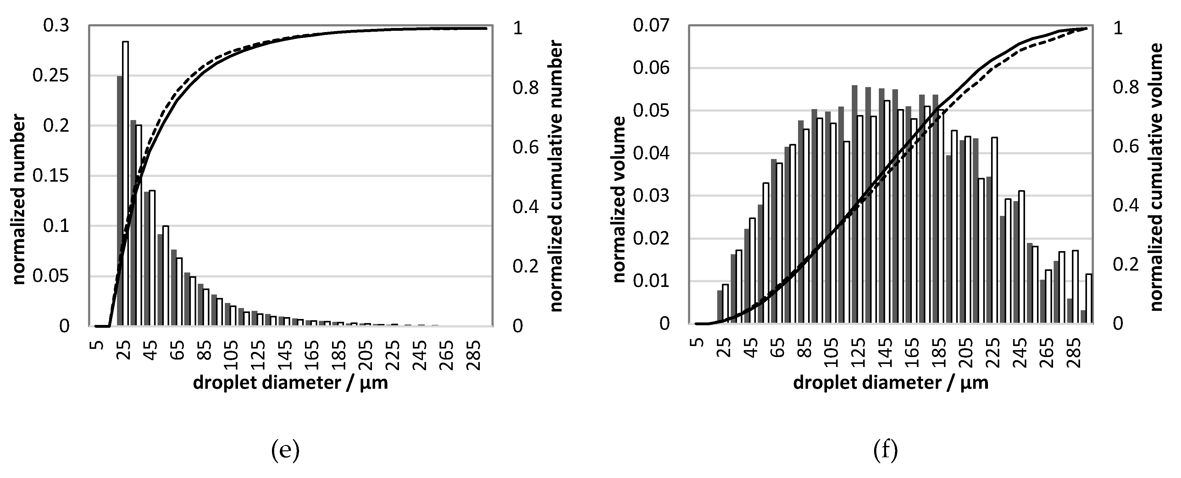
2.1.7. Droplet Size Distribution
2.2. Numerical Simulations
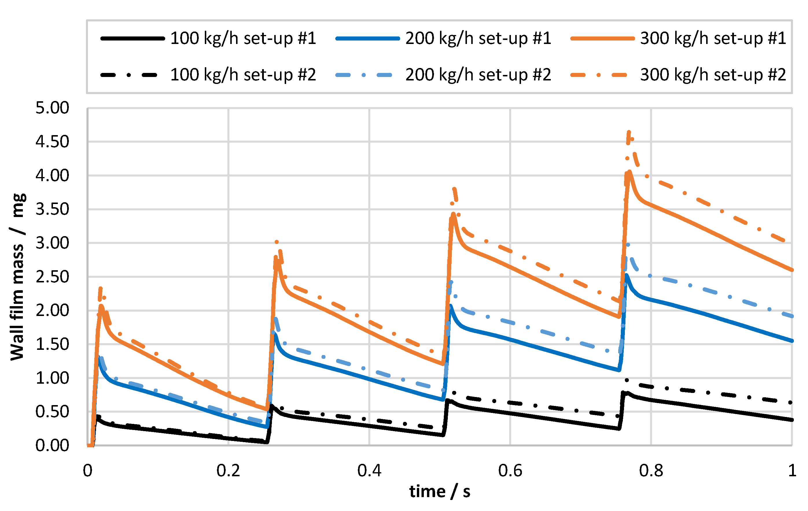
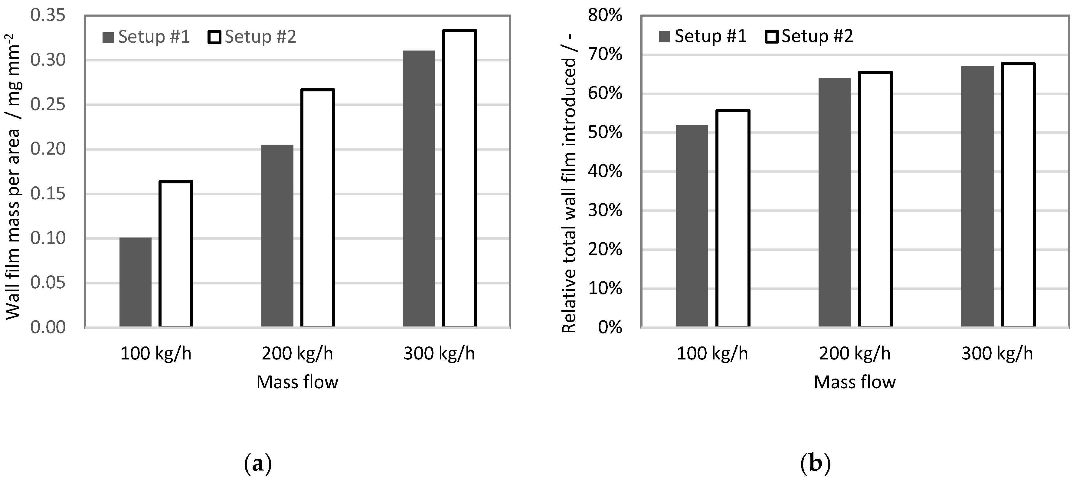
2.2.1. Wall Film Formation
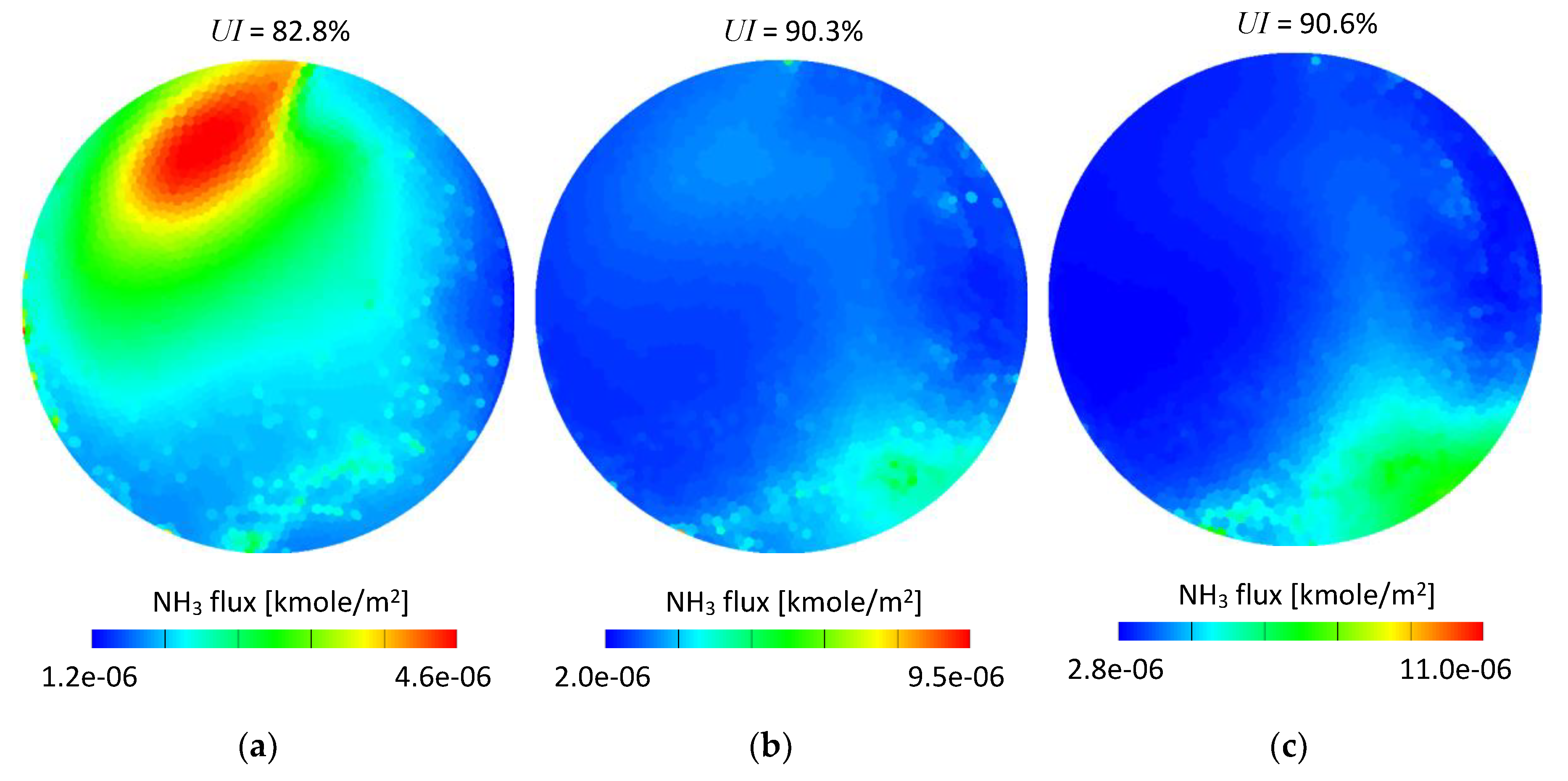
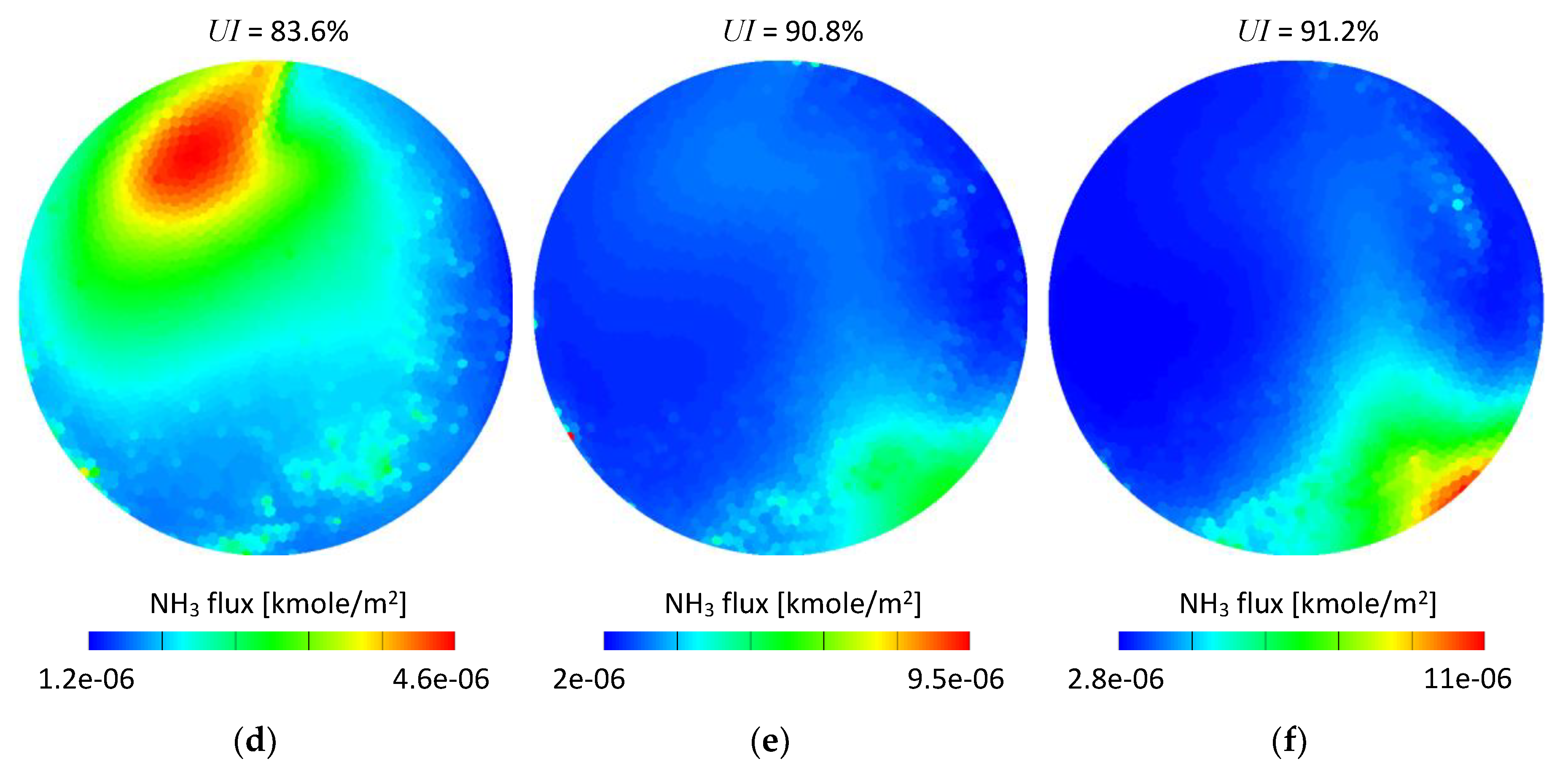
2.2.2. Ammonia Distribution
3. Materials and Methods
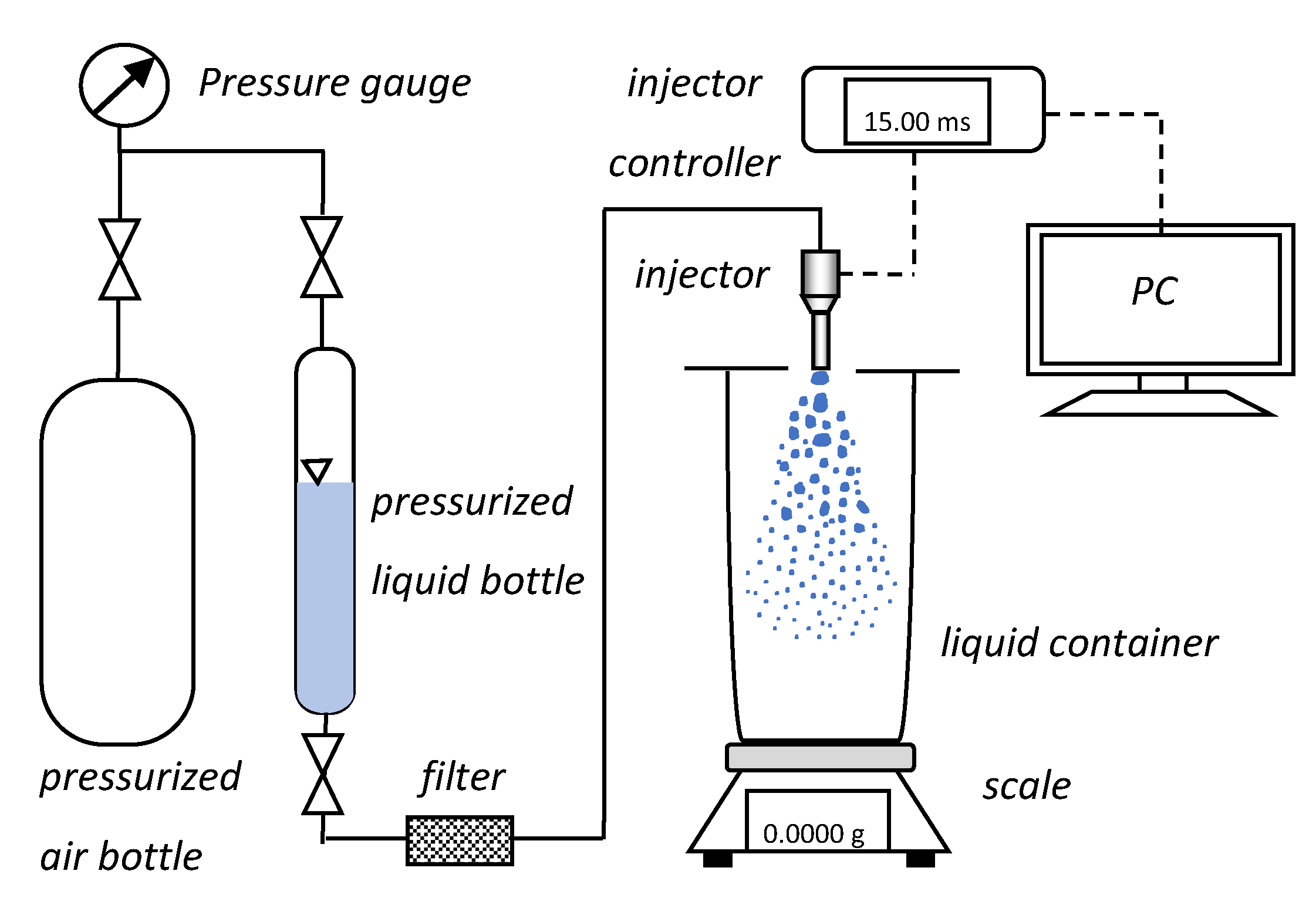
3.1. Experimental Set-Up
3.1.1. Flow Rate Measurement Set-Up
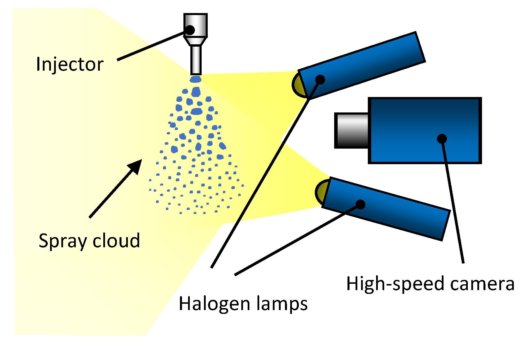
3.1.2. High-Speed Imaging
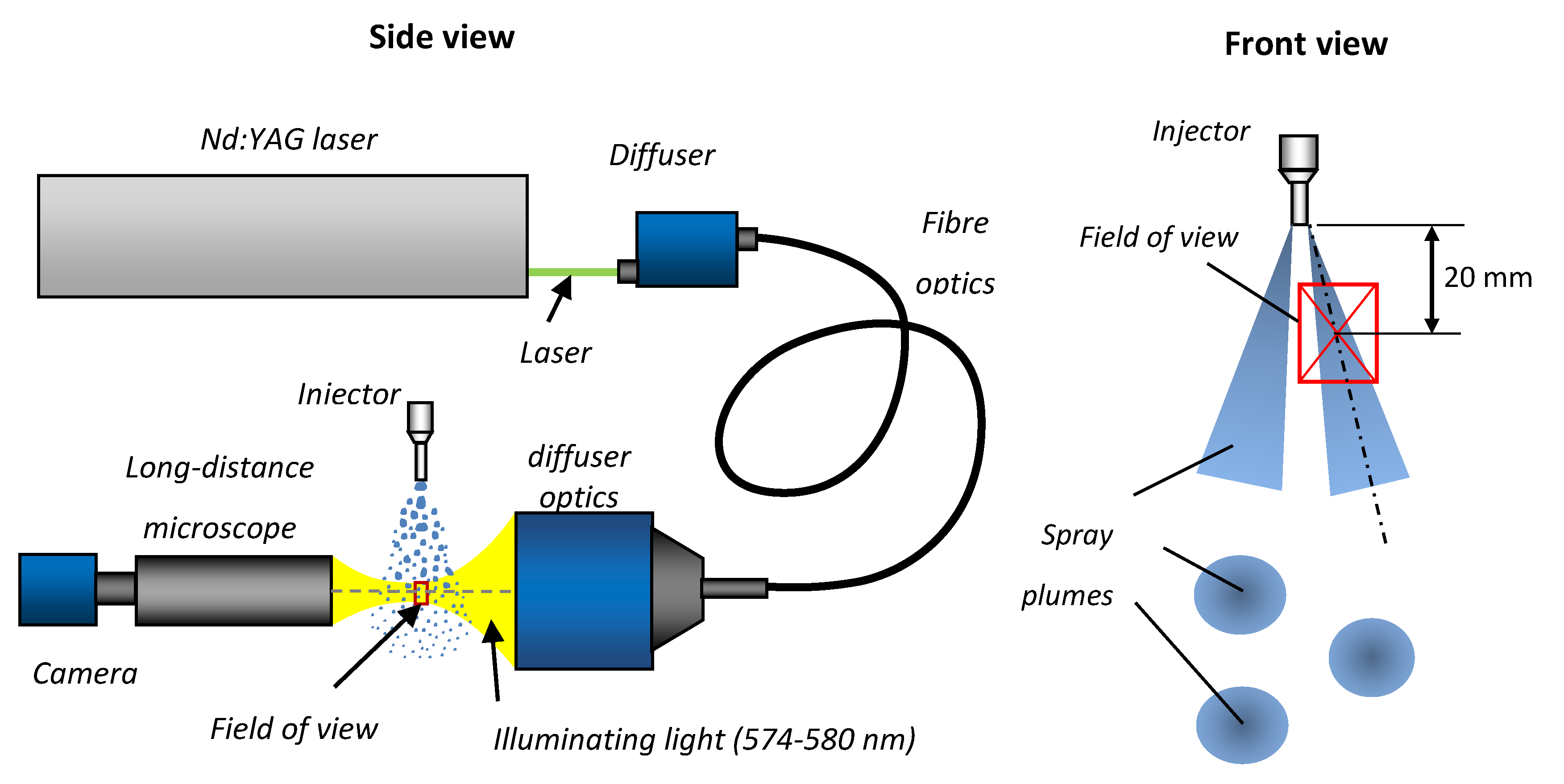
3.1.3. Shadowgraphy with a Long-Distance Microscope
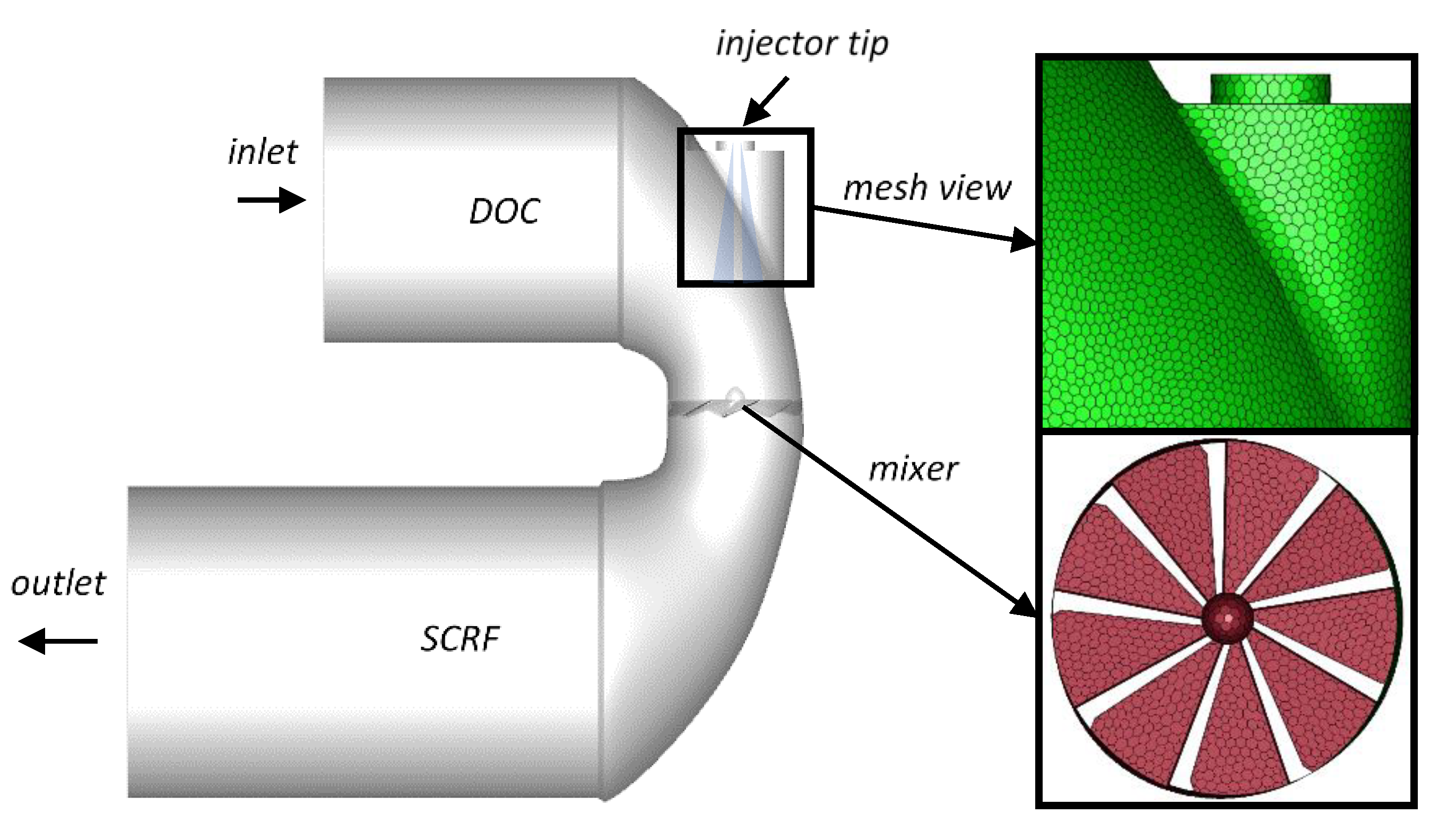
3.2. Numerical Simulations
4. Conclusions
Author Contributions
Funding
Acknowledgments
Conflicts of Interest
References
- Kojima, H.; Fischer, M.; Haga, H.; Ohya, N.; Nishi, K.; Mito, T.; Fukushi, N. Next Generation All in One Close-Coupled Urea-SCR System; SAE Technical Paper 2015-01-0994; SAE International: Warrendale, PA, USA, 2015. [Google Scholar]
- Sala, R.; Bielaczyc, P.; Brzezanski, M. Concept of vaporized urea dosing in selective catalytic reduction. Catalysts 2017, 7, 307. [Google Scholar] [CrossRef]
- Spiteri, A.; Eggenschwiler, P.D. Experimental fluid dynamic investigation of urea—Water sprays for diesel selective catalytic reduction—DeNOx applications. Ind. Eng. Chem. Res. 2014, 53, 3047–3055. [Google Scholar] [CrossRef]
- Baleta, J.; Vujanović, M.; Pachler, K.; Duić, N. Numerical modeling of urea water based selective catalytic reduction for mitigation of NOx from transport sector. J. Clean. Prod. 2014, 88, 280–288. [Google Scholar] [CrossRef]
- Varna, A.; Spiteri, A.C.; Wright, Y.M.; Dimopoulos, P. Experimental and numerical assessment of impingement and mixing of urea—Water sprays for nitric oxide reduction in diesel exhaust Q. Appl. Energy 2015, 157, 824–837. [Google Scholar] [CrossRef]
- Nocivelli, L.; Montenegro, G.; Liao, Y.; Dimopoulos, P. Modeling of aqueous urea solution injection with characterization of spray-wall cooling effect and risk of onset of wall wetting. Energy Procedia 2015, 82, 38–44. [Google Scholar] [CrossRef]
- Kapusta, Ł.J. LIF/Mie droplet sizing of water sprays from SCR system injector using structured illumination. In Proceedings of the ILASS2017–28th European Conference on Liquid Atomization and Spray Systems, Valencia, Spain, 6–8 September 2017. [Google Scholar]
- Kapusta, Ł.J.; Teodorczyk, A. Laser diagnostics for urea-water solution spray characterization. MATEC Web Conf. 2017, 118, 1–6. [Google Scholar] [CrossRef]
- Liao, Y.; Furrer, R.; Dimopoulos, P.; Boulouchos, K. Experimental investigation of the heat transfer characteristics of spray/wall interaction in diesel selective catalytic reduction systems. Fuel 2017, 190, 163–173. [Google Scholar] [CrossRef]
- CRC Handbook of Chemistry and Physics: A Ready-Reference Book of Chemical and Physical Data, 93rd ed.; Haynes, W.M. (Ed.) CRC Press: Boca Raton, FL, USA, 2012. [Google Scholar]
- International Organization for Standardization. Technical Report No. 22241-1:2019 Standard; ISO: Geneva, Switzerland, 2019. [Google Scholar]
- Halonen, S.; Kangas, T.; Haataja, M.; Lassi, U. Urea-water-solution properties: Density, viscosity, and surface tension in an under-saturated solution. Emiss. Control Sci. Technol. 2017, 3, 161–170. [Google Scholar] [CrossRef]
- Birkhold, F.; Meingast, U.; Wassermann, P.; Deutschmann, O. Analysis of the Injection of Urea-Water-Solution for Automotive SCR DeNOx-Systems: Modeling of Two-Phase Flow and Spray/Wall-Interaction; SAE Technical Paper 2006-01-0643; SAE International: Warrendale, PA, USA, 2006. [Google Scholar]
- Der Wiesche, S. Numerical heat transfer and thermal engineering of AdBlue (SCR) tanks for combustion engine emission reduction. Appl. Therm. Eng. 2007, 27, 1790–1798. [Google Scholar] [CrossRef]
- Ramires, M.L.V.; Nieto de Castro, C.A.; Nagasaka, Y.; Nagashima, A.; Assael, M.J.; Wakeham, W.A. Standard reference data for the thermal conductivity of water. J. Phys. Chem. Ref. Data 1995, 24, 1377–1381. [Google Scholar] [CrossRef]
- Bridgeman, O.C.; Aldrich, E.W. Vapor pressure tables for water. J. Heat Transfer 1964, 86, 279–286. [Google Scholar] [CrossRef]
- Ebrahimian, V.; Nicolle, A.; Habchi, C. Detailed modeling of the evaporation and thermal decomposition of urea-water solution in SCR systems. AIChE J. 2012, 58, 1998–2009. [Google Scholar] [CrossRef]
- Hale, G.M.; Querry, M.R. Optical constants of water in the 200-Nm to 200-μm wavelength region. Appl. Opt. 1973, 12, 555–563. [Google Scholar] [CrossRef]
- Polcar, A.; Čupera, J.; Kumbár, V.; Dostál, P.; Votava, I. Influence of urea concentration on refractive index of ad blue fluid evaluated by regression analysis. Acta Univ. Agric. Silvic. Mendelianae Brun. 2016, 64, 509–516. [Google Scholar] [CrossRef]
- Spiteri, A.; Srna, A.; Eggenschwiler, P.D. Characterization of sprays of water and urea-water solution from a commercial injector for SCR DeNOx applications. In Proceedings of the 13 Internationales Stuttgarter Symposium 2013 Automobil-und Motorentechnik, Stuttgart, Germany, 26–27 February 2013. [Google Scholar]
- Birkhold, F.; Meingast, U.; Wassermann, P.; Deutschmann, O. Modeling and simulation of the injection of urea-water-solution for automotive SCR DeNOx-systems. Appl. Catal. B Environ. 2007, 70, 119–127. [Google Scholar] [CrossRef]
- Grout, S.; Blaisot, J.-B.; Pajot, K.; Osbat, G. Experimental investigation on the injection of an urea–Water solution in hot air stream for the SCR application: Evaporation and spray/wall interaction. Fuel 2013, 106, 166–177. [Google Scholar] [CrossRef]
- Postrioti, L.; Brizi, G.; Ungaro, C.; Mosser, M.; Bianconi, F. A Methodology to investigate the behaviour of urea-water sprays in high temperature air flow for SCR de-NOx applications. Fuel 2015, 150, 548–557. [Google Scholar] [CrossRef]
- Payri, R.; Bracho, G.; Gimeno, J.; Moreno, A. Investigation of the urea-water solution atomization process in engine exhaust-like conditions. Exp. Therm. Fluid Sci. 2019, 108, 75–84. [Google Scholar] [CrossRef]
- Mie Simulator GUI; Virtual Photonics Technology Initiative: Irvine, CA, USA, 2019.
- Payri, R.; Bracho, G.; Gimeno, J.; Moreno, A. Spray characterization of the urea-water solution (UWS) injected in a hot air stream analogous to SCR system operating conditions. In WCX SAE World Congress Experience; SAE International: Detroit, MI, USA, 2019. [Google Scholar]
- Leroux, S.; Dumouchel, C.; Ledoux, M. The stability curve of newtonian liquid jets. Atom. Sprays 1996, 6, 623–647. [Google Scholar] [CrossRef]
- Dumouchel, C. On the experimental investigation on primary atomization of liquid streams. Exp. Fluids 2008, 45, 371–422. [Google Scholar] [CrossRef]
- Lin, S.P.; Reitz, R.D. Drop and spray formation from a liquid jet. Ann. Rev. Fluid Mech. 1998, 30, 85–105. [Google Scholar] [CrossRef]
- Ranz, W.E. On Sprays and Spraying; Department of Engineering Research, Pennsylvania State University: State College, PA, USA, 1956; Volume 65. [Google Scholar]
- Reitz, R.D.; Bracco, F.V. Mechanisms of breakup of round liquid jets. In Encyclopedia of Fluid Mechanics; Cheremisinoff, N.P., Ed.; Gulf Publishing Company: Houston, TX, USA, 1986; pp. 233–249. [Google Scholar]
- Baumgarten, C. Mixture Formation in Internal Combustion Engines, 1st ed.; Mewes, D., Mayinger, F., Eds.; Springer: Berlin/Heidelberg, Germany, 2006. [Google Scholar]
- Jaworski, P.; Kapusta, Ł.J.; Jarosiński, S.; Ziółkowski, A.; Capetillo, A.C.; Grzywnowicz, R. SCR systems FOR NOx reduction in heavy duty vehicles. J. KONES 2015, 22, 139–146. [Google Scholar] [CrossRef]
- Jaworski, P.; Jarosiński, S.; Kapusta, Ł.J.; Ziółkowski, A. SCR systems for NOx reduction in heavy and light duty vehicles. Combust. Engines 2016, 164, 32–36. [Google Scholar]
- Capetillo, A.; Ibarra, F. Multiphase injector modelling for automotive SCR systems: A full factorial design of experiment and optimization. Comput. Math. Appl. 2017, 74, 188–200. [Google Scholar] [CrossRef]
- Sala, R.; Dzida, J.; Krasowski, J. Ammonia concentration distribution measurements on selective catalytic reduction catalysts. Catalysts 2018, 8, 231. [Google Scholar] [CrossRef]
- Hanjalić, K.; Popovac, M.; Hadžiabdić, M. A robust near-wall elliptic-relaxation eddy-viscosity turbulence model for CFD. Int. J. Heat Fluid Flow 2004, 25, 1047–1051. [Google Scholar] [CrossRef]
- AVL FIRETM User Manual, Version 2014.2; AVL List GmbH: Graz, Austria, 2014.
- Gapin, A.; Demoulin, F.-X.; Dumouchel, C.; Pajot, K.; Patte-Rouland, B.; Reveillon, J. Development of an initial drop-size distribution model and introduction in a CFD code to predict spray evolution. In Proceedings of the 7th International Conferrence Multiph, Flow ICMF, Tampa, FL, USA, 30 May–4 June 2010. [Google Scholar]
- Kuhnke, D. Spray/Wall-Interaction Modelling by Dimensionless Data Analysis; Shaker Verlag: Herzogenrath, Germany, 2004. [Google Scholar]


| Parameter | Unit | Water | UWS |
|---|---|---|---|
| Density at 20 °C | g cm−3 | 0.9982 [10] | 1.0870–1.0930 [11] |
| Kinematic viscosity at 20 °C | mm2 s−1 | 1.0034 [12] | 1.2592 [12] |
| Kinematic viscosity at 30 °C | mm2 s−1 | 0.8007 [12] | 1.0127 [12] |
| Surface tension at 30 °C | N m−1 | 0.072 [13] | 0.075 [13] |
| Specific heat | kJ kg−1 K−1 | 4.2 [10] | 3.4 [14] |
| Thermal conductivity | W m−1 K−1 | 0.6 [15] | 0.57 [14] |
| Vapour pressure at 20 °C | kPa | 2.34 [16] | 2.05 [17] * |
| Refractive index | - | ~1.33 [18] | ~1.38 [19] |
| Injection Pressure (Gauge) MPa | Fluid Type | Static Mass Flow Rate g s−1 | Static Volumetric Flow Rate cm3 s−1 | Average Velocity in the Nozzle m s−1 | Re | Weg | Oh |
|---|---|---|---|---|---|---|---|
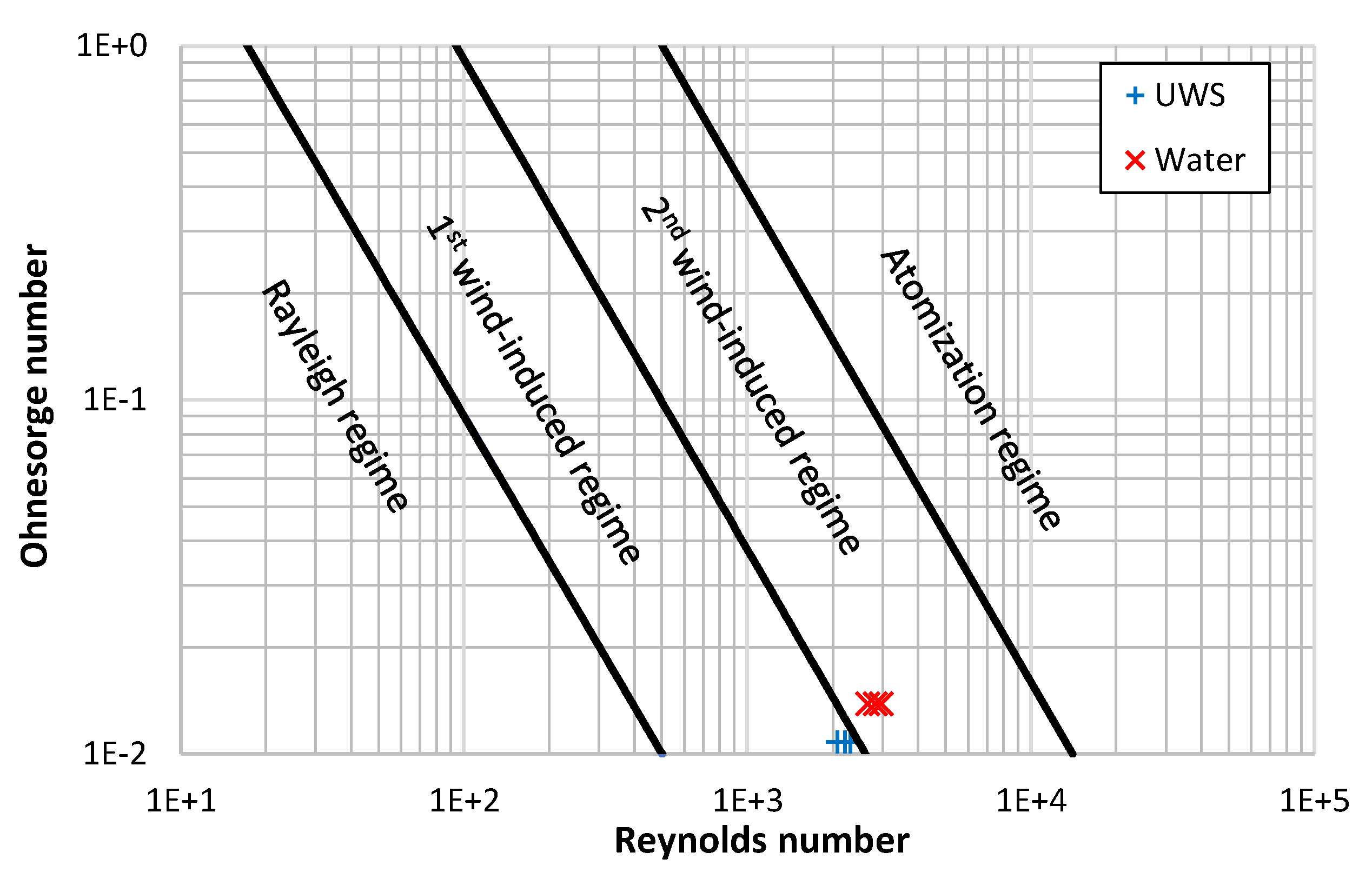
| 0.4 | UWS | 0.80 | 0.74 | 21.75 | 2073 | 0.91 | 0.0108 |
| 0.4 | Water | 0.75 | 0.75 | 22.22 | 2658 | 0.99 | 0.0139 |
| 0.45 | UWS | 0.85 | 0.78 | 23.12 | 2203 | 1.03 | 0.0108 |
| 0.45 | Water | 0.80 | 0.80 | 23.58 | 2820 | 1.12 | 0.0139 |
| 0.5 | UWS | 0.89 | 0.82 | 24.17 | 2303 | 1.13 | 0.0108 |
| 0.5 | Water | 0.84 | 0.84 | 24.76 | 2961 | 1.23 | 0.0139 |
| 0.4 MPa | 0.45 MPa | 0.5 MPa | |
|---|---|---|---|
| UWS | 24.5 | 25.1 | 26.1 |
| Water | 21.4 | 21.9 | 22.5 |
| Injection Pressure (Gauge) MPa | Fluid Type | Number of Droplets | DV10 µm | DV50 µm | DV90 µm | D32 µm |
|---|---|---|---|---|---|---|
| 0.4 | UWS | 8976 | 66.8 | 146.5 | 232.5 | 116.1 |
| 0.4 | Water | 10099 | 64.3 | 150.7 | 240.9 | 116 |
| 0.45 | UWS | 9606 | 63.8 | 142.5 | 233.2 | 112.2 |
| 0.45 | Water | 11381 | 59.2 | 146.5 | 240.9 | 110.4 |
| 0.5 | UWS | 12198 | 61 | 135.1 | 224.1 | 107.4 |
| 0.5 | Water | 12110 | 57.4 | 140.8 | 233.8 | 106.6 |
| Parameter | Unit | Set-up #1 | Set-up #2 |
|---|---|---|---|
| Inclination angle | deg | 6 | 6 |
| Single plume angle | deg | 7.3 | 5.4 |
| Static volumetric flow | cm3 s−1 | 0.82 | 0.84 |
| Initial jet velocity | m s−1 | 26.1 | 22.5 |
| Exhaust Gas Mass Flow | Exhaust Gas Temperature | NOx | UWS Dosage | Injector Opening Time Set-Up #1 (for UWS Flow Data) | Injector Opening Time Set-Up #2 (for Water Flow Data) |
|---|---|---|---|---|---|
| kg h−1 | °C | ppm | mg s−1 | ms | ms |
| 100 | 250 | 150 | 13.31 | 3.7 | 3.6 |
| 200 | 26.62 | 7.5 | 7.3 | ||
| 300 | 39.93 | 11.2 | 10.9 |
© 2019 by the authors. Licensee MDPI, Basel, Switzerland. This article is an open access article distributed under the terms and conditions of the Creative Commons Attribution (CC BY) license (http://creativecommons.org/licenses/by/4.0/).
Share and Cite
Kapusta, Ł.J.; Sutkowski, M.; Rogóż, R.; Zommara, M.; Teodorczyk, A. Characteristics of Water and Urea–Water Solution Sprays. Catalysts 2019, 9, 750. https://doi.org/10.3390/catal9090750
Kapusta ŁJ, Sutkowski M, Rogóż R, Zommara M, Teodorczyk A. Characteristics of Water and Urea–Water Solution Sprays. Catalysts. 2019; 9(9):750. https://doi.org/10.3390/catal9090750
Chicago/Turabian StyleKapusta, Łukasz Jan, Marek Sutkowski, Rafał Rogóż, Mohamed Zommara, and Andrzej Teodorczyk. 2019. "Characteristics of Water and Urea–Water Solution Sprays" Catalysts 9, no. 9: 750. https://doi.org/10.3390/catal9090750
APA StyleKapusta, Ł. J., Sutkowski, M., Rogóż, R., Zommara, M., & Teodorczyk, A. (2019). Characteristics of Water and Urea–Water Solution Sprays. Catalysts, 9(9), 750. https://doi.org/10.3390/catal9090750