Innovative Soft Computing Techniques for Analyzing Rate Constants in Artificial UV-Driven Photocatalysis Within Tubular Reactors

Abstract

Accurate prediction of photocatalytic degradation in TiO₂ reactors remains challenging due to the time-consuming, labor-intensive, and costly nature of experimental investigations, as well as the limited ability of conventional models. The degradation of benzoic acid was investigated in TiO₂-immobilized tubular plug-flow reactors under artificial UV radiation. The effects of reactor diameter and flow rate on the reaction rate constant were experimentally investigated. The results showed a constant reaction rate under artificial UV irradiation, which is attributed to higher electron photoactivation resulting in high photocatalytic activity. Three machine learning models, namely kernel extreme learning machine (KELM), Crested Porcupine Optimizer–Support Vector Regression (CPO-SVR), and Harris Hawks Optimizer (HHO)–SVR, were designed and compared for accurate prediction of reaction rates. The Pearson correlation coefficient (PCC), Willmott index (WI), Nash–Sutcliffe efficiency (NSE), and Legates–McCabe index (LM) were used to evaluate model performance. The highest predictive accuracy, resulting in the best PCC, WI, NSE, and LM values, was obtained from the HHO-SVR model, with PCC values of 0.990 and 0.990, WI values of 0.999 and 0.999, NSE values of 0.999 and 0.998, and LM values of 0.982 and 0.971 during training and testing, respectively. The CPO-SVR model also demonstrated good predictive performance and outperformed the KELM model on its own. A five-fold cross-validation ensured the stability and uncertainty of the HHO-SVR model. Shapley Additive Explanations (SHAP) analysis was used to determine the relative importance of operating parameters that affect the reaction rate over time, thereby enhancing model interpretability. The results showed the predominant factors controlling photocatalytic degradation and how these factors influenced the model predictions.

1. Introduction

The contamination of water with organic pollutants has emerged as a major environmental problem, mainly due to rapid industrialization, urbanization, and the high volume of hazardous chemicals released into water bodies. Some conventional treatment technologies are not very effective at removing persistent organic compounds, so advanced oxidation processes (AOPs) are considered sustainable solutions. Xia et al. studied organic wastewater treatment using a microwave-assisted UV/TiO₂ photocatalytic system, and examined the impact of operating parameters on the wastewater treatment efficiency. They showed an increase in degradation efficiency, but they did not address predictive modeling of reaction kinetics or predict and optimize the degradation process kinetics [1]. Walsem et al. designed a high-efficiency multi-tube UV photoreactor and used CFD modeling to simulate the adsorption and photocatalytic degradation of acetaldehyde. The model was well-matched with experimental data and could predict reactor behavior reasonably well, but was only valid for the reactor configuration and the experimental operating conditions [2]. Amakiri and Khan examined the latest developments in photocatalytic wastewater treatment, particularly regarding reactor design, process optimization, and the integration of photocatalysts to enhance wastewater treatment efficiency. They noted that photocatalytic processes were scalable, but raised concerns about catalyst recovery, operational stability, and scale-up [3]. Likewise, Fang et al. conducted degradation experiments and CFD simulations to understand the effects of flow-field configuration and hydrodynamic parameters on photocatalytic degradation in a reactor with TiO₂-coated tube walls. Their findings showed that the improved reactor geometry and flow conditions had a very positive effect on degradation efficiency, though predictive machine learning kinetic modeling was not explored [4].

Photocatalytic oxidation technology has attracted considerable interest due to its ability to mineralize organic contaminants into innocuous end products, such as carbon dioxide and water [5]. Titanium dioxide (TiO₂) is one of the most used photocatalysts due to its high chemical stability, low toxicity, strong oxidizing ability, and low cost. Numerous studies have been conducted on the usage of photocatalytic reactors for wastewater treatment with UV radiation [6].

Alhamdan et al. [7] compared different lamp configurations and operating conditions for 185 nm VUV irradiation of PFBA degradation to overcome the drawbacks of conventional oxidation processes. Three different LED-based UV photoreactors of varying irradiation configurations (direct, internal, and external) were constructed and used to test the degradation of phenol with TiO₂ under the same conditions, with the results showing that significant differences existed in energy efficiency due to design and temperature effects, and standard radiometric measurements did not accurately predict the actual performance of the real photoreactors. The internal radiation was the most efficient at 97.79%, suggesting the importance of reactor design, though it was limited to a single type of contaminant under batch conditions [8]. Blou developed a multidimensional approach to modeling the kinetics of photocatalytic reactions, accounting for interactions among multiple operating parameters. They have developed a framework that enhances kinetic analysis but does not use predictive modeling with machine learning [9]. Savage et al. created a machine learning-assisted CFD- and Bayesian-optimization-based framework with the help of additive manufacturing to investigate high-dimensional reactor geometries, and successfully arrived at 60% improved plug-flow design with an optimized vortex-enhanced coiled reactor design, albeit one constrained by CFD cost, simplified reactor scope, and surrogate-model dependency [10]. Solout and Ghasemi built GCN, GAT, and GAT–GCN models using the molecular structure and features of the photocatalysis process to predict the degradation rates of TiO₂, with GAT being the best model (R² = 0.90), though it was limited by dataset size and applicability to TiO₂ [11]. Na et al. applied RF, XGB, and LGB models to 618 data points from 89 studies, arriving at pseudo-first-order chemical degradation rate constants from the features of operating conditions and pollutants, and showed that XGB was the most accurate, with power density and frequency being the most important features; however, the data were highly heterogeneous and relied on literature-based values [12].

Several operating parameters, such as irradiation intensity, flow rate, reactor geometry, catalyst loading, and hydraulic conditions, significantly affect the efficiency of the photocatalytic process [13]. Thus, accurate prediction of reaction rate constants is key to reactor design, process optimization, scale-up, and operational control. The relationships between the transport phenomena, light distribution, mass transfer processes, and photocatalytic reactions.

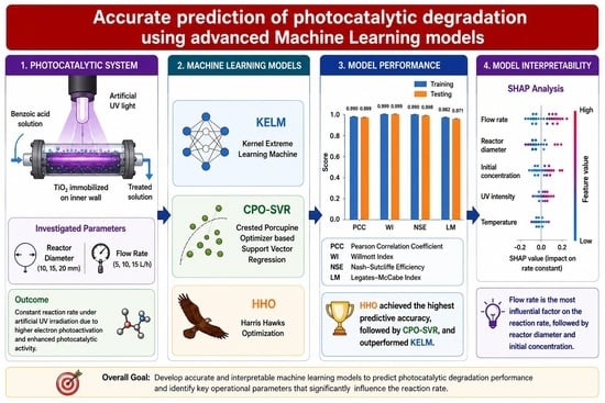
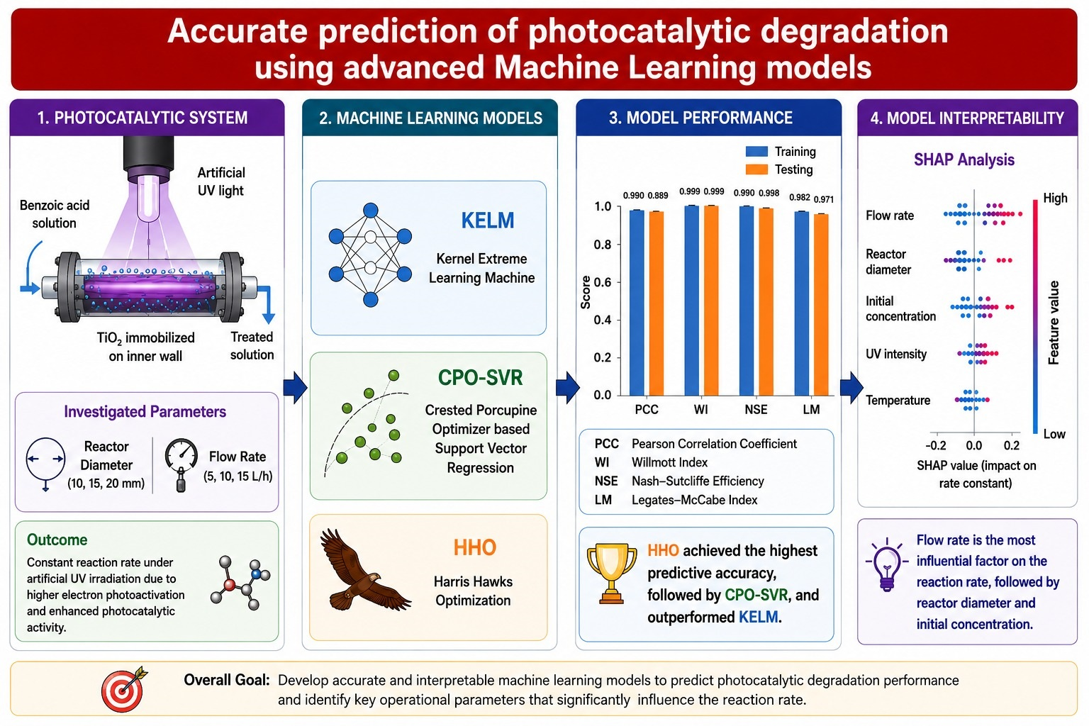
This study aims to develop and compare the soft computing models KELM, CPO-SVR, and HHO-SVR for predicting the reaction rate constant for the degradation of benzoic acid in photocatalytic tubular reactors with immobilized TiO₂, with the reactor irradiated using a UV source. Multiple statistical performance measures were employed to train and test the various models with experimental data under different operating conditions. Moreover, the most influential process variables for controlling photocatalytic degradation were identified using SHAP analysis. The proposed framework integrates advanced machine learning and metaheuristic optimization, enabling the creation of an accurate and interpretable tool for analyzing, optimizing, and applying photocatalytic reactors to improve water treatment processes, specifically for sustainable water treatment.

2. Research Gap and Novelty Study

Photocatalytic oxidation has been extensively studied for wastewater treatment applications; many previous studies have focused primarily on degradation performance, the efficiency of the catalyst, and the design of the reactor, with little attention to exact and accurate prediction of the photocatalytic reaction rate constants using advanced ML techniques. Most of the models developed so far have been unable to capture the complex nonlinear interactions among irradiation conditions, flow rate, reactor geometry, and photocatalytic activity. Only a limited number of studies have combined modern optimization algorithms from the fields of metaheuristics and machine learning with photocatalytic analysis.

The selection of ML architecture heavily depends on the model’s convergence property. Traditional ML models, e.g., random forest and XGBoost, rely on locally greedy tree-based splitting criteria. Initially, these models converge quickly during training. However, these models struggle to model continuous physical parameters. These models use stepwise decision planes and lack an explicit mechanism to optimize using continuous, smooth parameters. Therefore, they struggle to generalize to continuous data and are prone to overfitting. A recent graph convolutional network (GCN) can generate a topological graph structure within data points. However, backpropagation convergence might be unstable when applied to tabular continuous data, making it computationally complex and susceptible to over-parameterization.

In contrast, this study uses an SVR model. SVR is superior at handling noisy data because it uses the structural mean across the data distribution. But SVR needs to find global minima within its hyperparameter space, i.e., regularization (C), tube width (ε), and kernel radius (γ). Adjustment of these parameters can determine a nonlinear boundary for prediction. Most traditional frameworks, e.g., grid search or random search, are limited in their applicability due to quantization errors and computational complexity. An alternative approach is a probabilistic-based approach, i.e., Bayesian optimization. However, it may easily get stuck in local minima with complex nonlinear data and converge prematurely if the data are noisy. In addition, the interpretability of machine learning predictions has not been well-explored in photocatalytic reactor studies.

Thus, the novelty of the present work lies in the development of an integrated soft computing framework comprising a kernel extreme learning machine (KELM) and metaheuristic-optimized SVR models. Metaheuristic optimization avoids a derivative-free search space mechanism. This approach dynamically balances global exploration and exploitation. We proposed Crested Porcupine Optimizer–Support Vector Regression (CPO-SVR) and Harris Hawks Optimizer–Support Vector Regression (HHO-SVR) for accurate prediction of the reaction rate constants in UV-driven TiO₂-immobilized tubular reactors.

Furthermore, SHAP analysis quantifies the contribution of each operating variable, thereby making the model more transparent and providing physical insight into the factors governing the photocatalytic degradation process. This comprehensive solution provides a novel, accurate, and interpretable design tool for reactors, process optimization, and intelligent water treatment applications.

3. Results and Discussion

3.1. Normal Distribution Analysis for the Input and Output Variables

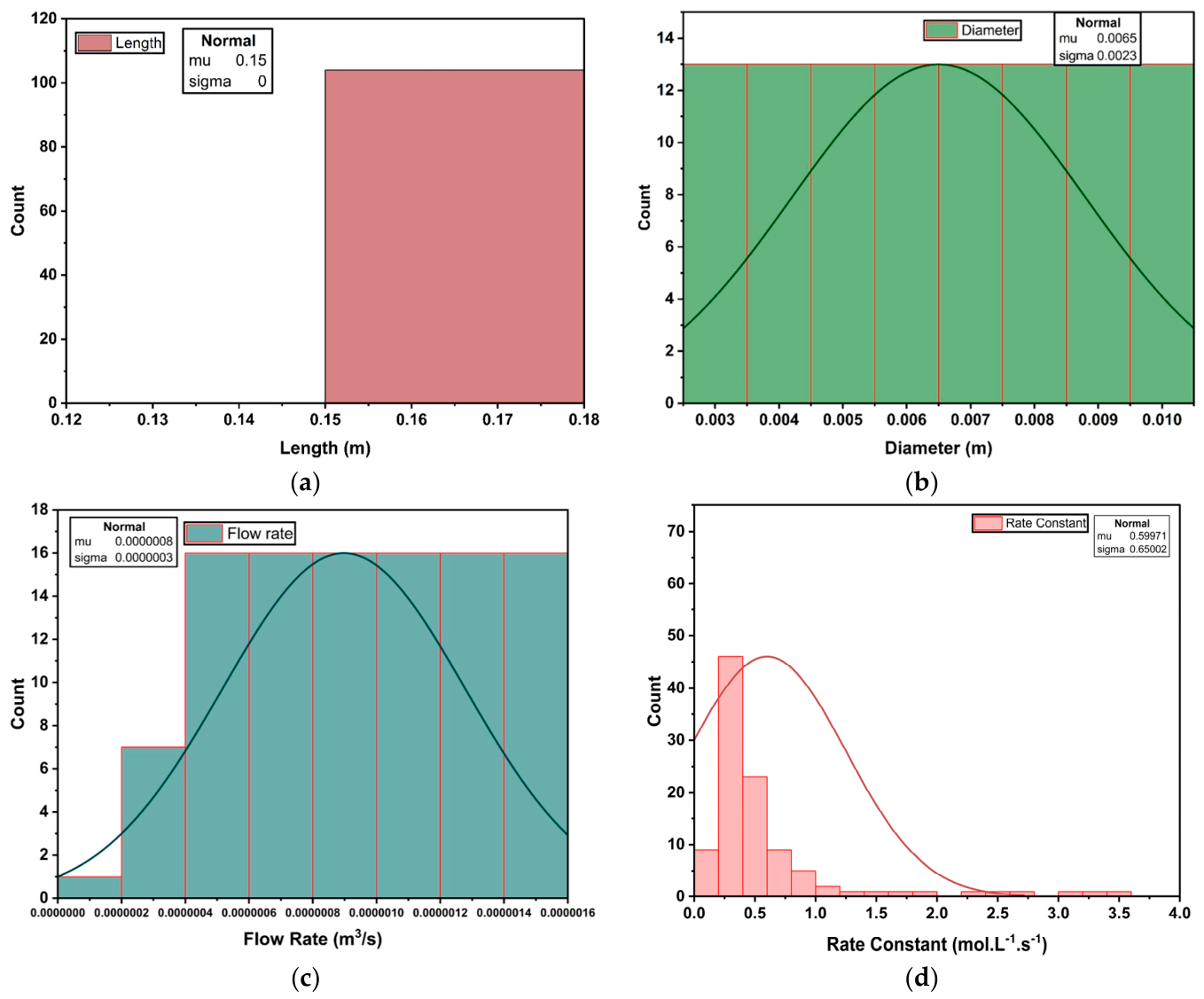
Figure 1 shows the normal distribution for the input and output values. The length measurements are concentrated at 0.15 m. The diameter varies from 0.003 m to 0.010 m in eight discrete scales, as shown in the histogram of Figure 1b. Each bin represents the sample frequency, i.e., 13 counts or experiment trials for each diameter. It shows a Gaussian-like distribution with a peak at 0.0065 m and a low standard deviation of 0.0023 m, indicating high precision in the measurement process. Figure 1c shows the flow rate count distribution across designated volumetric velocity intervals. It has 16 experimental trials per bin across the higher operational spectrum ranging to 1.6 × 10⁻⁶ m³/s. The flow rate distribution shows a similar Gaussian trend, as the data are concentrated around a single peak at 8.974 × 10⁻⁷ m³/s, with a standard deviation of 3.810 × 10⁻⁷ m³/s, providing useful information about the flow rate under the experimental conditions. The rate constant has a right-skewed profile, with 65 observations residing between 0 and 0.5 m/s, with a peak at velocities around 0.5 m/s and a standard deviation of 0.650 m/s, reflecting the range of parameters observed during experimentation. These numbers together help clarify the complex nature of the measured physical properties and provide a sound statistical basis for future analysis.

3.2. Performance of KELM

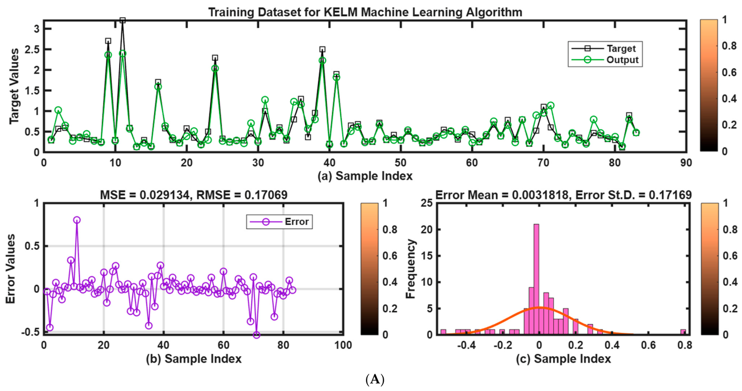
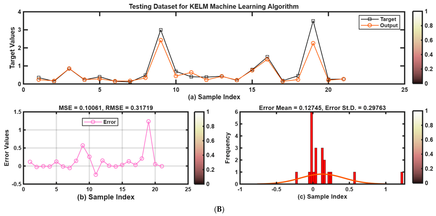
KELM is used as a base model. The KELM is configured with a radial basis function (RBF) kernel, which is the best-performing kernel for handling nonlinear data. A regularization coefficient (C) and a kernel bandwidth (γ) determine KELM’s predictive stability. As noted, we used a five-fold cross-validation strategy, and C = 10 and γ = 5 for the first fold yielded the best results. Figure 2 shows the prediction results for both training and test datasets.

3.3. Performance of Metaheuristic-Optimized SVR (CPO-SVR and HHO-SVR)

Both CPO and HHO optimized the three hyperparameters of SVR. These include the regularization parameter C, the kernel parameter γ, and the insensitive loss parameter ϵ. Each combination was verified, and the one that yielded the lowest MSE was used as the optimal value.

Table 1. Hyperparameter ranges of SVR and their optimized values using CPO and HHO models.

Hyperparameter	Lower Bound (lb)	Upper Bound (ub)	Optimized Value
			CPO	HHO
C	0.1000	1000.0000	894.8165	396.7348
γ	0.0001	10.0000	2.54	1.4517
ε	0.0010	1.0000	0.0010	0.0146

lists the initial ranges of these parameters and their corresponding optimal values.

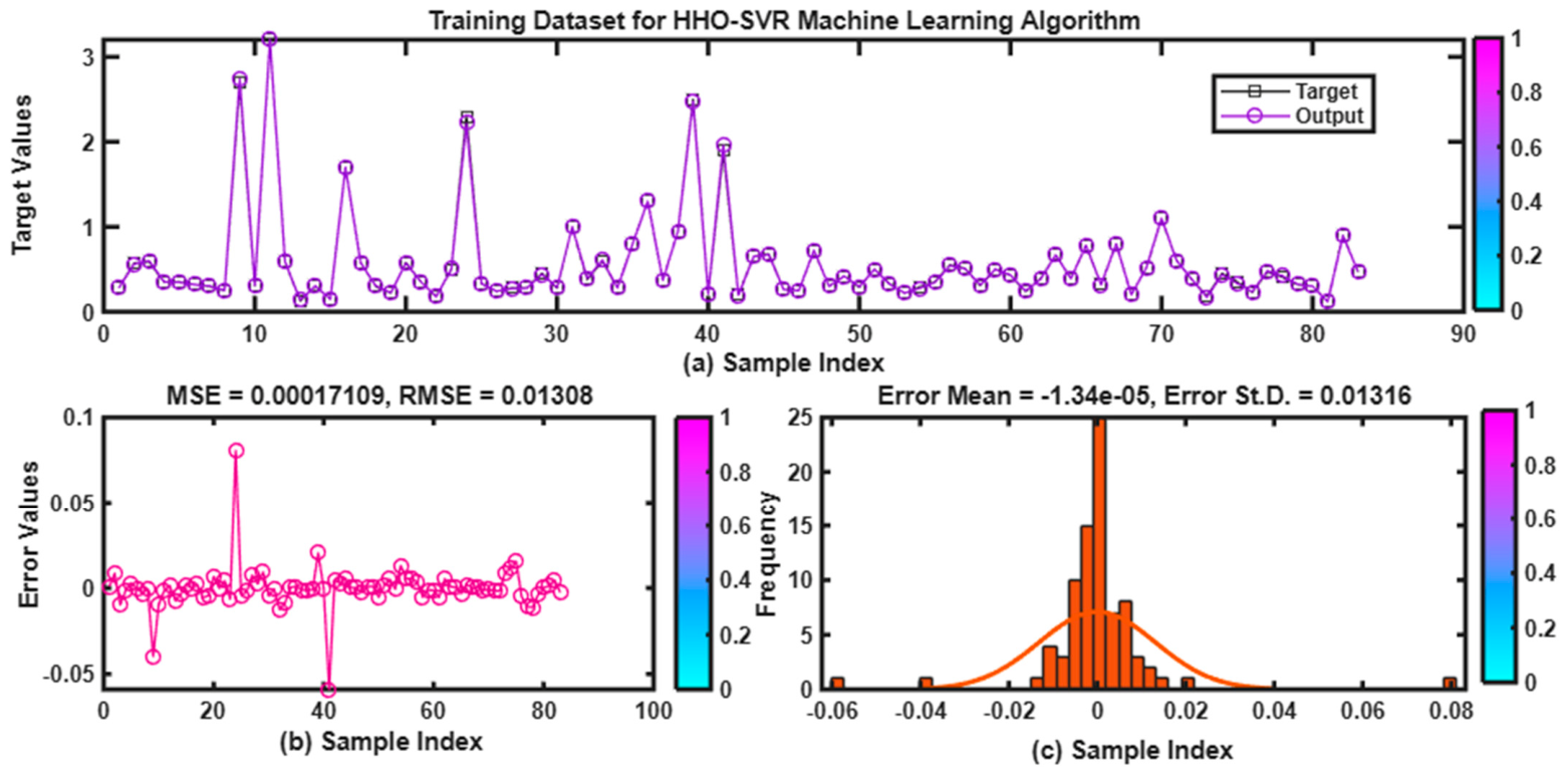
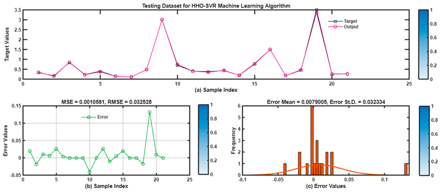
Figure 3 and Figure 4 illustrate the performance of the HHO-SVR on the training and test datasets, showing the model’s target values. For the range of sample indices, the predicted values and their degree of agreement with the target values are displayed in Figure 3a. It is evident that the model is not overfitting to a small number of sample values and has successfully learned the underlying relationship across the range of index values. The error metrics reported in Figure 3b are quantitative measures of the accuracy of the model’s predictions, such as MSE = 0.00017109 and RMSE = 0.01308, which are small, indicating that deviations between the model’s predictions and the targets are small on the training set. The residual errors in Figure 3c are randomly distributed around zero, with no obvious long-range systematic trend, suggesting good overall stability in the general fit of the samples. The overall bias, with an error mean = −1.34 × 10⁻⁵, is negligible, as the model slightly underestimates on average. The histogram shows the distribution of prediction errors, which has a relatively small spread error (St. D. = 0.01316) and is clustered around zero. This error distribution indicates that the model is quite accurate, as most predictions fall within a relatively small range of the actual values. This indicates that the model is suitable for prediction tasks and that its predictions do not deviate significantly from the actual values.

Figure 4a prediction shows that the model learned well from the training data and exhibits no overfitting. The deviations are within a limited range, as indicated by the testing error metrics: MSE = 0.0010581 and RMSE = 0.032528. The error vs. sample index in Figure 4b also reveals that prediction errors cluster around a small mean value rather than systematically increasing or decreasing across all test set samples, indicating no predominant error pattern throughout the test set. This is verified quantitatively by the error statistics, where the mean error was 0.0079005, indicating a slight positive bias. And the error standard deviation of 0.032334 indicates that the errors are not widely spread. Finally, the error histogram in Figure 4c shows that errors cluster around zero with a single dominant frequency, indicating that errors were within a relatively small range.

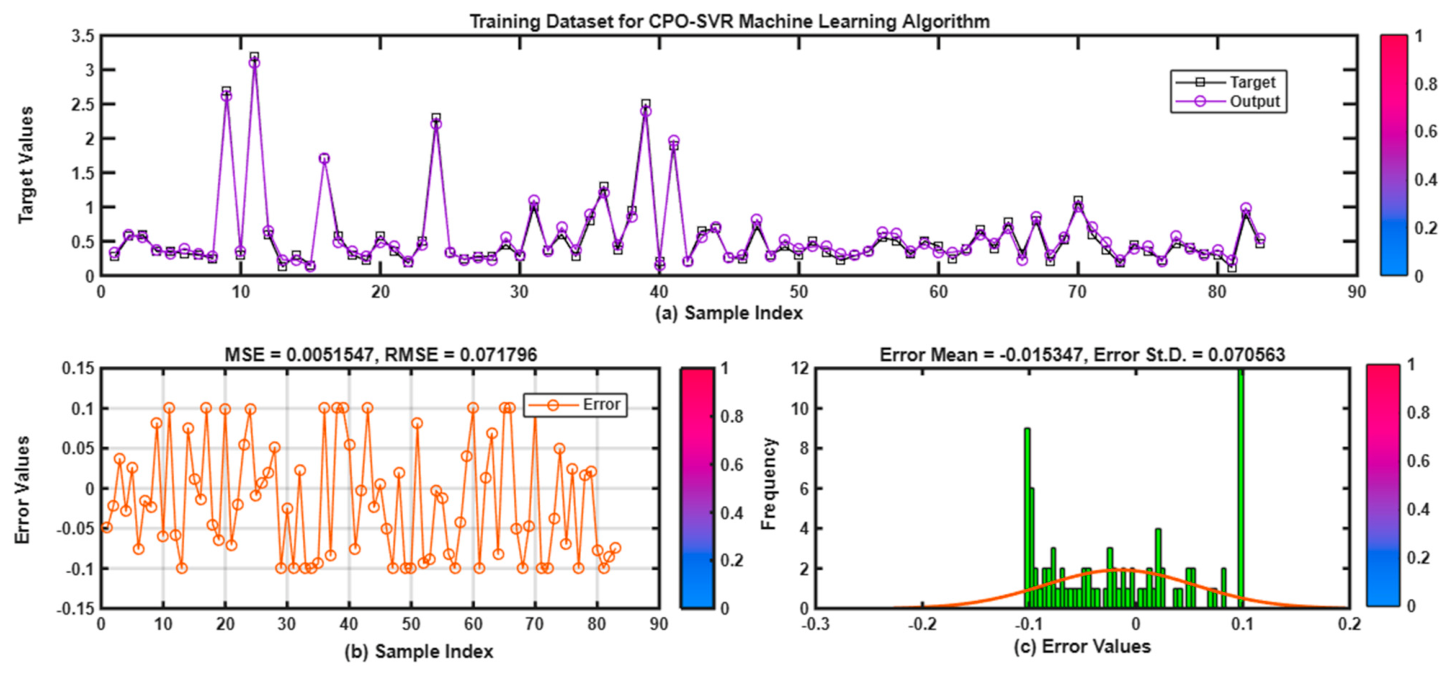
Figure 5a illustrates the performance evaluation of the CPO-SVR machine learning algorithm model on the training dataset. The predicted values closely overlap with the target values across all training samples, indicating that the model accurately captures the nonlinear relationship between the input and output. Figure 5b illustrates the prediction errors for each sample, with residuals randomly distributed around zero without any noticeable systematic pattern, indicating the absence of significant bias. The low MSE (0.00515) and RMSE (0.07180) further confirm the model’s high predictive accuracy. Moreover, the error histogram in Figure 5c exhibits an approximately normal distribution centered near zero, with a mean of −0.01535 and a standard deviation of 0.07056, indicating minimal prediction bias and low variability. It demonstrates that the CPO-SVR model is robust, reliable, and capable of accurately learning the underlying patterns in the training dataset.

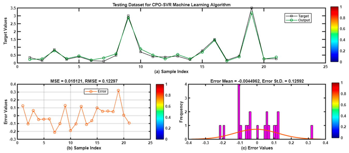
Figure 6 presents the predictive performance of the CPO-SVR model on the testing dataset. The predicted values closely match the corresponding target values for all test samples, demonstrating the model’s excellent generalization capability and its ability to accurately predict unseen data, as shown in Figure 6a. Although slight deviations are observed for a few samples, particularly near the higher output values, the overall agreement remains strong. Figure 6b shows that the prediction errors are randomly distributed around zero with no systematic trend, indicating that the model does not exhibit significant bias. The low MSE (0.01512) and RMSE (0.12297) further confirm the model’s satisfactory predictive accuracy on the test dataset. Moreover, the error histogram shown in Figure 6c exhibits an approximately normal distribution, with a mean error of −0.00450 and a standard deviation of 0.12592, suggesting negligible prediction bias and acceptable error variability.

3.4. Evaluation of Metric Analysis for the Machine Learning Models

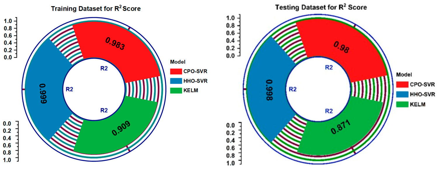
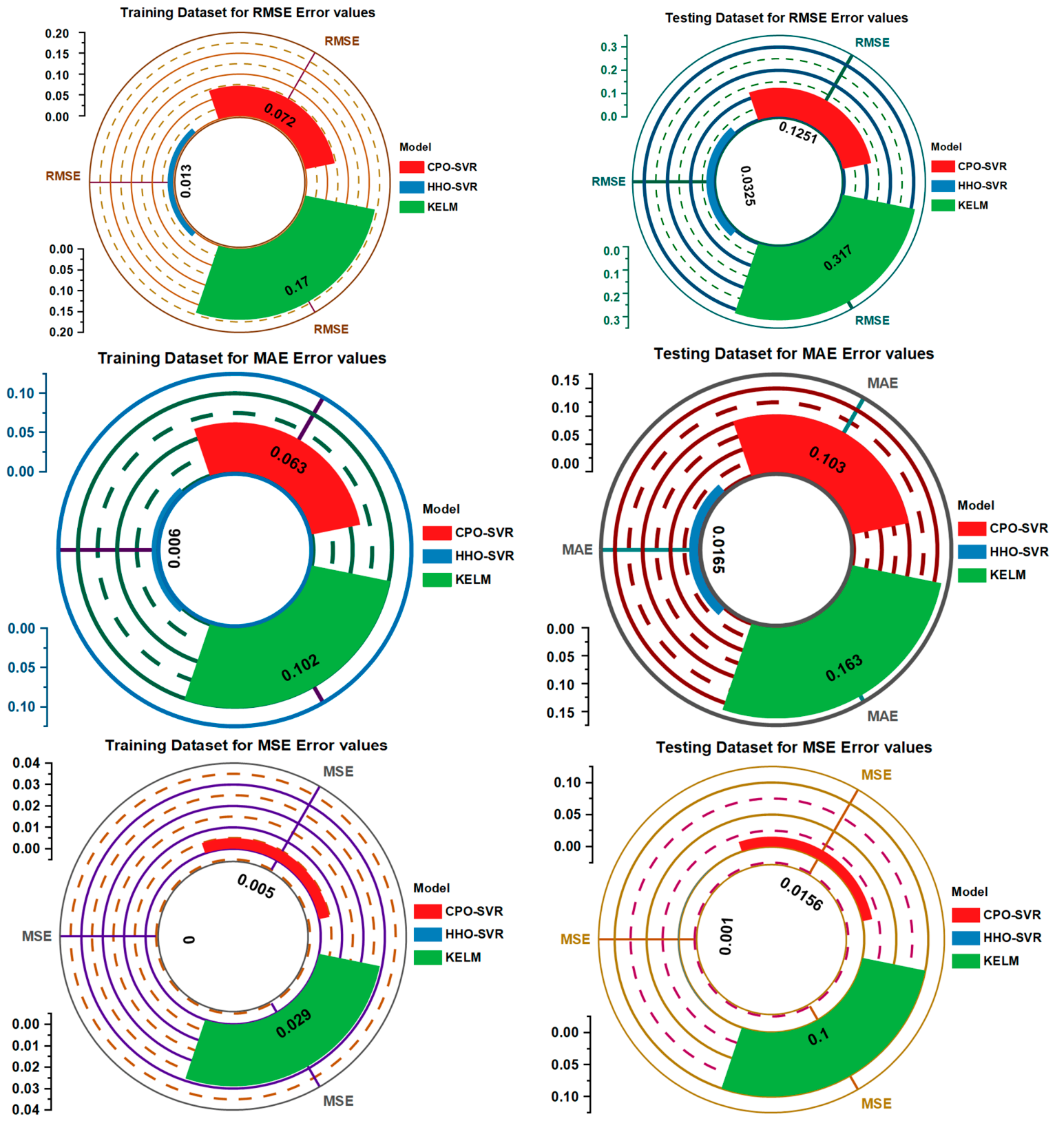
Figure 7 displays the performance parameters of the models CPO-SVR, HHO-SVR, and KELM, which provide insight into their predictive ability. The R² scores for SVR with CPO and HHO are consistent across the training and test datasets. In contrast, KELM has the lowest R² values, indicating that it might not be as effective as in fitting the data. Prediction error statistics using MAE, RMSE, and MSE indicate that both CPO-SVR and HHO-SVR have lower prediction errors than KELM. Furthermore, HHO-SVR received the lowest error score among all methods.

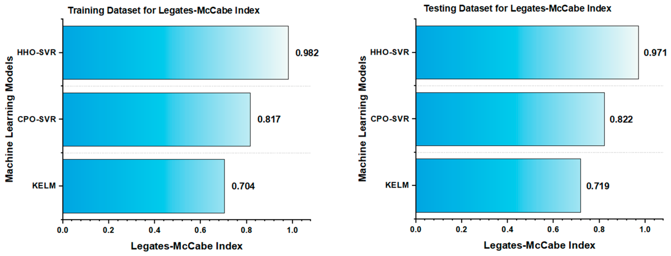
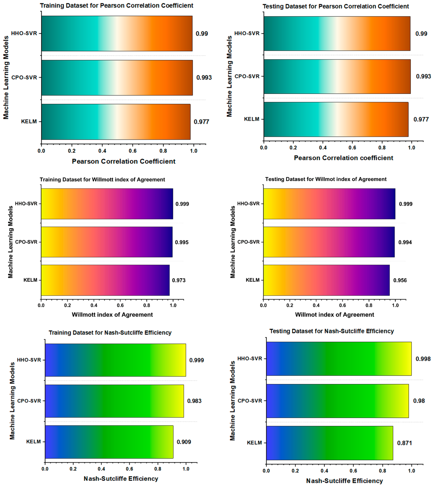
Figure 8 comprehensively compares the three machine learning models—HHO-SVR, CPO-SVR, and KELM—using performance metrics, including the Pearson correlation coefficient, Willmott index of agreement, Nash–Sutcliffe efficiency, and Legates–McCabe index. The Pearson correlation coefficient for HHO-SVR is consistently higher than for the other models, indicating that it identifies relationships in the data better than the others, with CPO-SVR being the next best. KELM tends to perform worse. The Willmott index of agreement shows the same pattern, with HHO-SVR having near-perfect scores, indicating a high degree of agreement between the predicted and observed values. CPO-SVR is competitive but slightly lower and KELM is significantly lower. These observations are confirmed by the Nash–Sutcliffe efficiency metrics, with HHO-SVR once again as the top performer (close to one), and KELM having the lowest values for all metrics. Lastly, in the Legates–McCabe index analysis, HHO-SVR is the most reliable, while CPO-SVR and KELM are less reliable, especially on the test set. In general, these results confirm that the HHO-SVR model is the best, followed by the CPO-SVR model, while the KELM model consistently performs worse across the evaluated metrics.

3.5. Regression Plots for the Machine Learning Models

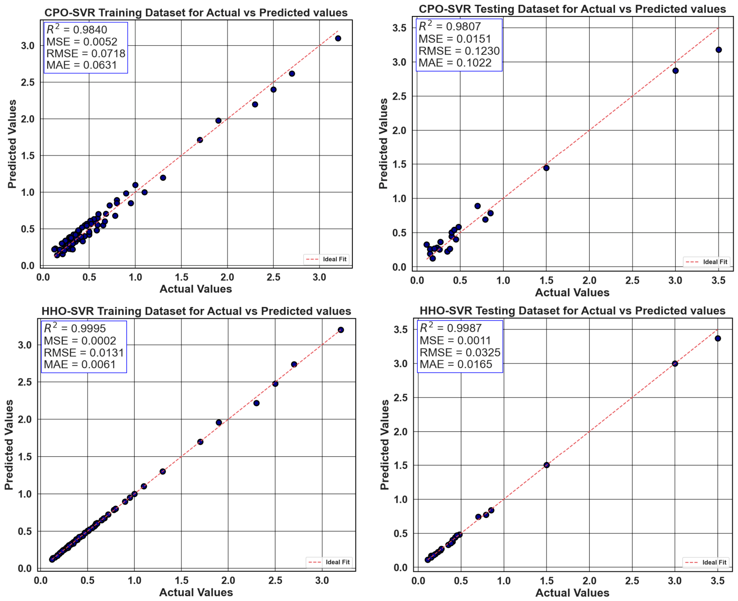
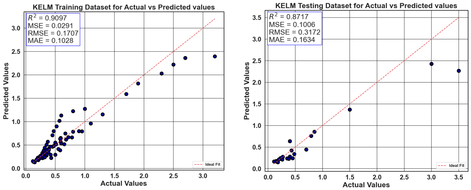
Figure 9 shows the regression scatter plots of actual vs. predicted values for both the training and testing sets of KELM, CPO-SVR, and HHO-SVR. Among the three models, the HHO-SVR machine learning algorithm shows very good predictive performance. The R² score for the training set is 0.9995, which is very close to the perfect 1, with a very low mean square error (MSE) of 0.0002, a root mean square error (RMSE) of 0.0131, and a mean absolute error (MAE) of 0.0061. These statistics indicate that HHO-SVR is a good model of the underlying relations in the training set and is very close to the truth. The model has a high R² of 0.9987, with a close correspondence between the actual and predicted values in the test set. MSE rises slightly to 0.0011, while RMSE is 0.0325 and MAE is 0.0165, indicating that although there is a slight increase in error compared to the training phase, the model continues to demonstrate high accuracy. In general, the values predicted on both plots are close to the ideal fit line, supporting the HHO-SVR model’s ability to make accurate predictions across various datasets.

3.6. Comparison of Machine Learning Models

A single split of the data into training and test sets with a random partition may lead to varying performance. Therefore, the models’ generalization and reliability are validated using a five-fold cross-validation.

Table 2. Model reliability tests using five-fold cross-validation.

		KELM				CPO-SVR				HHO-SVR
Fold	Dataset	R2	MSE	RMSE	MAE	R2	MSE	RMSE	MAE	R2	MSE	RMSE	MAE
1	Train	0.909	0.029	0.170	0.102	1.00	0.00	0.000	0.0006	0.996	0.001	0.031	0.028
	Test	0.871	0.100	0.317	0.163	0.950	0.038	0.191	0.077	0.988	0.008	0.093	0.053
2	Train	0.904	0.034	0.180	0.10	1.000	0.000	0.000	0.0006	0.999	0.000	0.013	0.006
	Test	0.844	0.126	0.354	0.120	0.959	0.026	0.161	0.125	0.998	0.001	0.032	0.016
3	Train	0.942	0.022	0.151	0.086	1.000	0.000	0.000	0.0006	0.992	0.003	0.054	0.045
	Test	0.704	0.139	0.372	0.233	0.536	0.217	0.466	0.248	0.954	0.021	0.146	0.090
4	Train	0.930	0.035	0.187	0.120	0.983	0.005	0.072	0.063	0.999	0.000	0.007	0.006
	Test	0.641	0.008	0.093	0.071	0.980	0.015	0.125	0.103	0.974	0.0006	0.025	0.020
5	Train	0.944	0.027	0.166	0.095	1.000	0.000	0.000	0.0007	1.000	0.000	0.0007	0.0007
	Test	0.019	0.061	0.247	0.142	0.942	0.003	0.060	0.041	0.953	0.022	0.148	0.102

shows the models’ performance for each fold for both the training and test datasets. KELM shows consistent performance on the training set but low performance on the test set, suggesting overfitting. Fold 1 showed the best results among all folds. CPO-SVM outperformed KELM across all folds, achieving a competitive error rate. But the performance (R² score) on the test set could not improve beyond 0.96. In contrast, HHO-SVR showed consistent and robust performance among all folds. For fold 5, both KELM and CPO-SVM performance deviate significantly on the test set, but HHO-SVR maintained its baseline performance, with an R² score of 0.95. This clearly shows that HHO-SVR performed better than CPO.

Table 3. Training and testing datasets for R², RMSE, MAE, and MSE.

Model	Dataset	R2	RMSE	MAE	MSE
KELM	Training	0.909	0.170	0.102	0.029
	Testing	0.871	0.317	0.163	0.100
CPO-SVR	Training	0.983	0.072	0.063	0.005
	Testing	0.980	0.1251	0.103	0.0156
HHO-SVR	Training	0.999	0.013	0.006	0.000
	Testing	0.998	0.0325	0.0165	0.001

illustrates the best performance of all models on the training and test datasets. The KELM model has moderate performance, with R² = 0.90 in training and R² = 0.871 in testing, indicating its efficacy is not as high as that of the other models. The error in its predictions is high, as shown by RMSE values of 0.170 and 0.317 for training and testing, respectively. MAEs for the training and testing sets were 0.102 and 0.163, respectively. MSEs for the training and testing data were 0.029 and 0.100, respectively. However, CPO-SVR performed better compared to KELM, with R² values of 0.983 for training and 0.980 for testing, demonstrating its ability to model the data pattern, which is desirable for this task. It has a low RMSE of 0.072 for training and 0.1251 for testing, indicating that the predicted values are closer to the actual values. Overall, the MAE and MSE were also lower, i.e., (0.063, 0.103) and (0.005, 0.0156), for the training and testing data.

HHO-SVR was the best-performing model among KELM and CPO-SVR, with a training R² of 0.999 and a testing R² of 0.998. The RMSE values for the test and training sets were very low, at 0.0325 and 0.013, respectively, and the smallest MAE (0.0165 and 0.006) and MSE (0.001 and 0.000) were achieved. Such measures all highlight the superiority of HHO-SVR over KELM and CPO-SVR.

Table 4. Performance metrics PCC, WI, NSE, and LM for training and testing dataset.

Model	Dataset	PCC	WI	NSE	LM
KELM	Training	0.957	0.973	0.909	0.704
	Testing	0.977	0.956	0.871	0.719
CPO-SVR	Training	0.992	0.995	0.983	0.817
	Testing	0.993	0.994	0.980	0.822
HHO-SVR	Training	0.990	0.999	0.999	0.982
	Testing	0.990	0.999	0.998	0.971

presents the performance metrics for KELM, CPO-SVR, and HHO-SVR across the training and testing datasets, providing significant insights into their predictive capabilities. The Pearson correlation coefficient (PCC) for KELM is 0.957 during training and 0.977 during testing, indicating a strong linear relationship between the predicted and true values. The Willmott index (WI) is also strong, with training scores of 0.973 and testing scores of 0.956. The Nash–Sutcliffe efficiency (NSE) drops from 0.909 during the training phase to 0.871 during the testing phase, indicating less precise predictions in the latter stage. Finally, the Legates–McCabe index (LM) shows an average performance, with scores of 0.704 and 0.719 on training and test data, respectively. The performance of CPO-SVR is better than KELM. The PCC on the training set is 0.992 and, on the test, set is 0.993. The WI is excellent, 0.995 for training, 0.994 for testing, and the model is consistent. The NSE values are also high, at 0.983 and 0.980 in the training and testing sets, respectively, indicating good predictive accuracy. However, the LM score is limited to 0.817 and 0.822, respectively, though it showed improved performance over KELM. HHO-SVR showed exceptional performance on training and test datasets with PCC, WI, and NSE scores around 0.99. The LM for HHO-SVR increased to 0.982 on the training data and 0.971 on the testing data, further bolstering the model’s forecasting prowess. Overall, HHO-SVR performs very consistently and accurately in all metrics when compared to KELM and CPO-SVR.

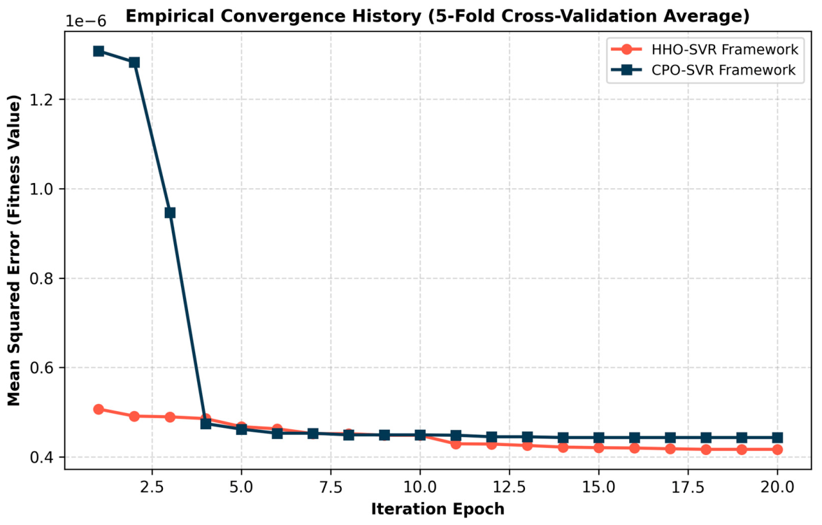
The two optimization algorithms are further evaluated by analyzing their convergence speed and optimization efficacy. Figure 10 shows the five-fold MSE as a function of the number of training epochs. It shows that CPO-SVR has a steep exploration descent from iterations 2 to 4, and later remains stable with no further progress. In contrast, HHO-SVR begins with a more promising search space and continuously refines it. It achieved a drop in MSE from iteration 11 onwards. Thus, it converged to a lower MSE of 0.41 × 10⁻⁶ compared to CPO-SVR and demonstrated better exploitation capacity.

HHO’s superior performance over CPO lies in its global search exploration capability for nnonlineardatasets. Photocatalytic data is highly nonlinear and noisy. HHO calculates the escaping energy of the prey ($E=2E_0\left(1-{\displaystyle \frac{t}{T}}\right)$), which is a decreasing function over the iteration; where E0 fluctuates between −1 and 1 for each step, and E switches between. This random fluctuation prevents HHO from converging on local minima and shifts it toward a global search during the optimization cycle. Thus, E switches the population between exploratory and exploitative states throughout the runtime. During the hunting phase, E is paired with the Levy flight distribution function. It provides short-step movement followed by a sudden long jump. Thus, it allows easy, fast escape from the trap of fitting within the local valley. CPO’s structural behavior relies on the transition from the localized neighbor-bound reflection matrix. These localized transitions may lose population diversity in a high-variance search space, leading to premature convergence due to noisy data. Therefore, HHO succeeded in capturing the true optimal values of the hyperparameters, while retaining the flexibility to explore the global space. This is also validated in Figure 10.

3.7. SHAP Analysis for the Experimental Input and Output Variables

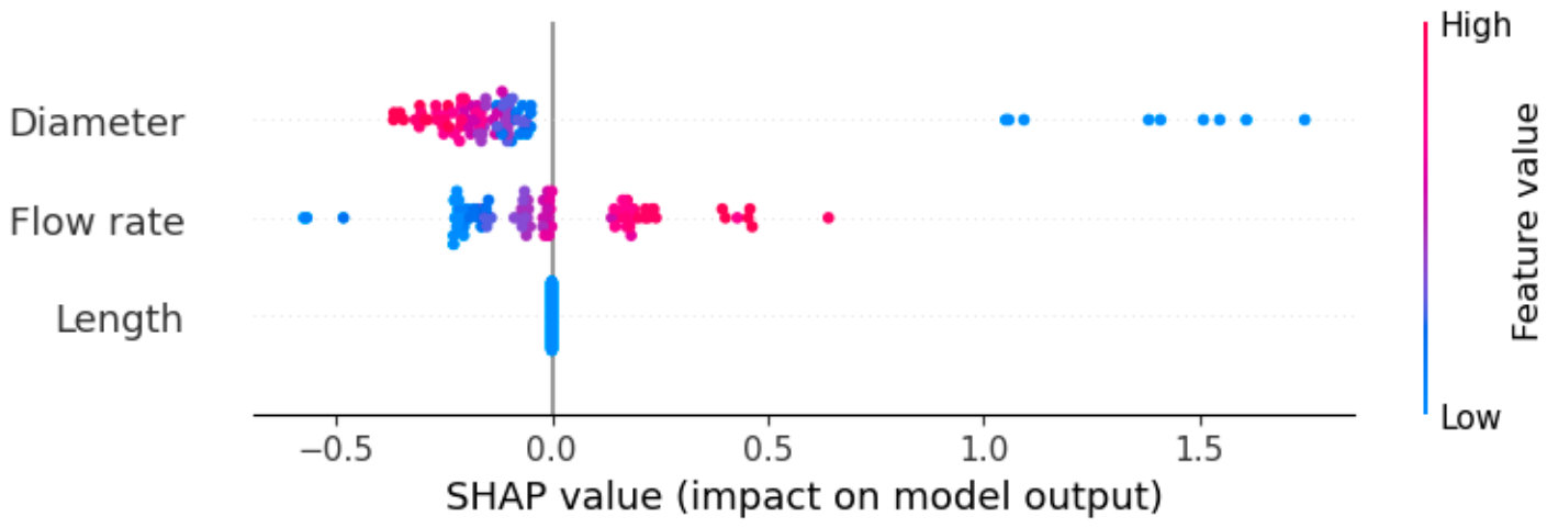
Figure 11 shows the SHAP summary plot, which graphically represents each feature’s impact on the model’s output, the direction of its effect on the prediction, and its magnitude. The points represent SHAP values for individual samples; those to the right of zero indicate that higher values of the corresponding feature tend to lead to higher predictions, whereas a higher value of the corresponding feature tends to lead to a lower prediction for points with SHAP values on the left side of zero.

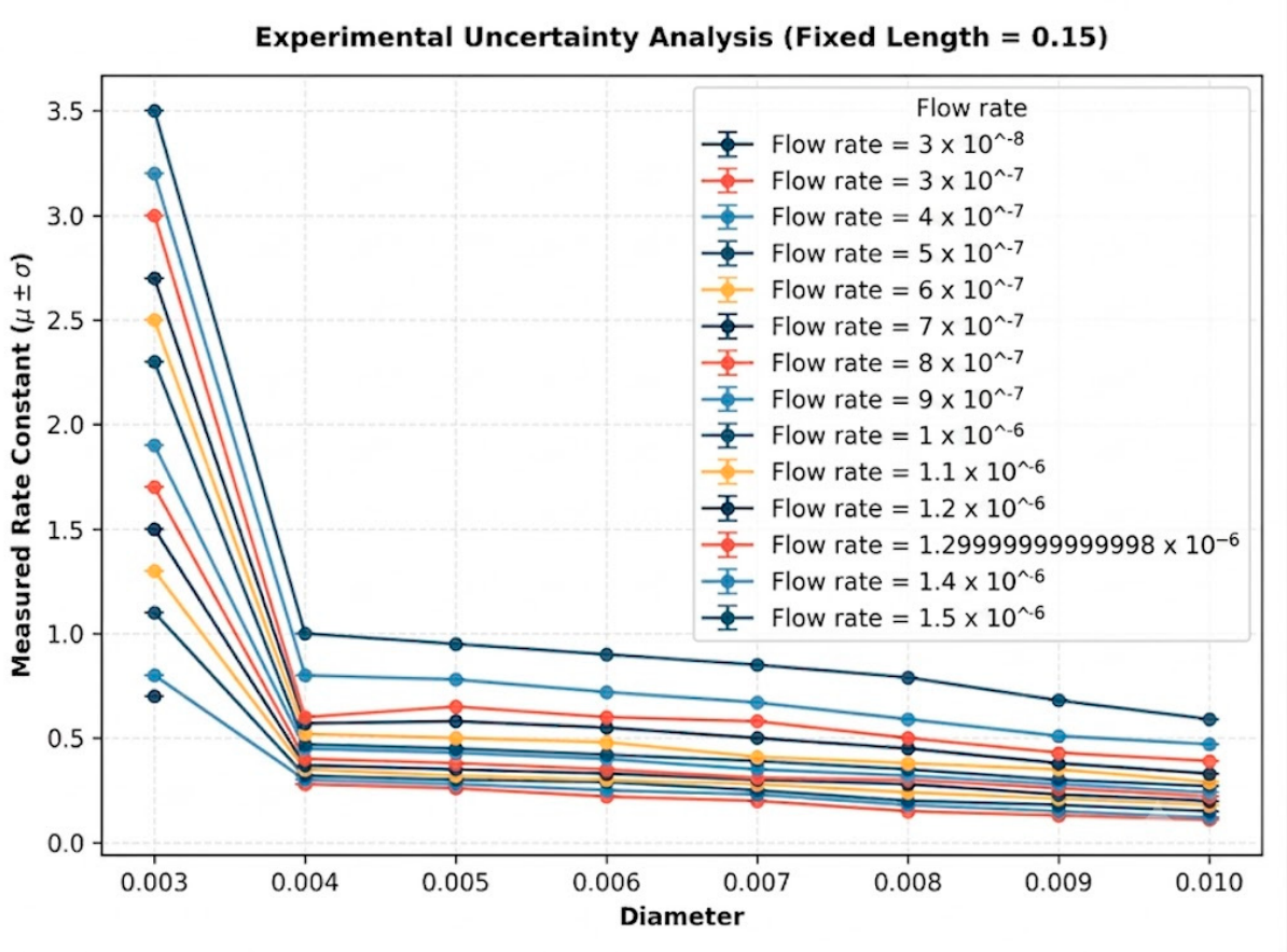
Diameter is the most widely used of the three, serving as the dominant parameter for predicting the rate constant. The large values are tightly coupled to the left and negatively correlated with the target. In contrast, the low diameter values yielded positive SHAP values up to +1.75. UV light penetration depth and internal mass transfer constraints are the main causes of this behavior. The Beer–Lambert Law suggests that the exponential decay of UV photon intensity occurs from the outer surface to the central region. Due to the large diameter, the center zone remains unilluminated, and the catalyst remains inactive. Narrowing the diameter to a small scale allows UV light to fully penetrate the entire fluid cross-section. This full penetration maximizes the volumetric photon absorption rate. A small diameter increases the surface-area-to-volume ratio of the reactor. Thus, it drastically increases the probability of the physical contact between the liquid-phase reactants and the wall-immobilized photocatalyst. Additionally, it reduces the internal diffusion path length that a reactant molecule in the bulk fluid must traverse to reach an active catalytic site. This transition reduces the internal mass resistance and drastically increases the rate constant, as shown in Figure 12, at a fixed length of 0.15. Figure 12 shows that for a diameter greater than 0.4, the dark zone is dominant, and the rate constant is low; however, lowering the diameter to 0.003 causes a sudden increment in the rate constant from 0.75 to 3.5. The flow rate shows a bidirectional relationship. It shows the competitive mechanics between residence time and external mass transfer dynamics. The low flow rate, or alternatively, slow fluid movement, creates a thick hydrodynamic boundary layer along the reactor wall. This layer creates a physical diffusion barrier and strangles the reaction rate.

Table 5. Comparison of machine learning models from past literature with those in the current study.

ML Models Used	Sources	Metric Scores	Ref.
SVM, ANN, tree-based models, RF, XGB, LGB	Photocatalysis wastewater treatment datasets, using TiO2, ZnO, CdS, Zr, WO2, and CeO2 catalysts	R2 > 0.95, RMSE = 0.02	[14]
XGB, DT, LR2, SVR, AB, VR, CB, KNN, GB, RF, ANN, RR, LR	Literature-based TiO2 photocatalytic air pollutant degradation	R2 = 0.94 for XGB, DT, LR2; R2 = 0.63 for LR, RR, ANN; best RMSE = 0.49, MAE = 0.29	[15]
Hybrid metaheuristic–RF models (TSA-RF, HFA-RF, HHA-RF, NRO-RF, DEA-RF, LSA-RF)	TiO2 photocatalytic degradation dataset for air contaminants (UV-assisted, 200 data points from experiments)	TSA-RF—R2 = 0.90, RMSE = 0.25; HFA-RF/HHA-RF/NRO-RF—R2 = 0.88, RMSE = 0.32; lowest was DEA-RF/LSA-RF—R2 = 0.85, RMSE = 0.45	[16]
ANN, Gaussian process (GP), Support Vector Machine (SVM)	rGO–SnS2 photocatalyst wastewater degradation dataset	ANN—R2 = 0.97, error = 0.002; GP & SVM showed lower accuracy compared to ANN	[17]
KELM, CPO-SVR, HHO-SVR, optimization-based ML models	TiO2-immobilized tubular plug-flow reactor dataset for benzoic acid degradation under artificial UV Lamp (60 W)	Best: HHO-SVR (PCC = 0.990, WI = 0.99, NSE = 0.99, LM = 0.982); CPO-SVR showed strong performance	Present study

compares details from the previous literature with the current study’s investigation using machine learning models.

4. Materials and Methods

4.1. Materials

Benzoic acid, sodium hydroxide, and TiO₂ photocatalyst were procured from Merck, Germany.

4.2. Experimental Facility

The tank is installed on top of the stand, and a 60 W artificial ultraviolet lamp is connected to the frame in this test installation. The capacity of the tank is 0.10 × 0.15 × 0.10 m. A UV lamp is mounted on a frame, with adjustable positioning via a nut, bolt, and bush, which facilitates downward and upward movement. Small tubes are installed at a slight slope to keep the flow moving by gravity. An elbow fitter was used to connect a 0.5″ copper tube to the outlet of the tank. Gate valves are installed at the inlets of the glass tubes, which are connected to the copper tube. The different tube lengths correspond to different tube diameters of tubes coated with an immobilized photocatalyst [18]. To create the desired flow network, ½ inch T-connectors were used to join the copper tube. There were two ½″ elbow connectors, one from the outlet of the tank to the inlet of the copper pipe, and another from the end of the copper pipe to the fifth glass pipe’s gate valve. Additionally, four ½ inch T-connectors were used to join the copper pipes with the gate valves of the glass pipes. Five gate valves were inserted to control the water movement in each glass pipe. In addition, five pipe reducers were placed to reduce the size of the connection from ½ to ¼ inch for the glass pipes to be properly attached between the gate valves and the glass inlets. The tank outlet with a copper tube and the photocatalytic reactor tubes with various dimensions are connected to the main copper tube with slight inclination (same angle for all tubes) for smooth gravity flow. Once the flow rate was fixed by using gate valve in the main copper tube, same flow passes through all the photocatalytic reactor tubes. The UV intensity and pollutant concentration is kept constant for a particular flow rate. This study is fixed on the degradation of model pollutant component, that being benzoic acid. The experimental dataset consists of 3 independent and 1 dependent variable: length (m), diameter (m), flow rate (m³/s), and rate constant (mol·L⁻¹·s⁻¹). A total of 104 experimental datasets were employed to design the machine learning model. In this model, 80% of the datasets were used for training, and the remaining 20% for testing to predict the target value. To prevent overfitting in robust optimization, a 5-fold cross-validation strategy is employed within the optimization loops of both CPO and HHO. The 80% training dataset is divided into five equal subsets, and four of these subsets are used to train the SVR. The MSE across all five validation datasets is used as the fitness function. To ensure that the parameters’ extreme values were uniformly distributed and to avoid localized data skewing, a random shuffle with a fixed random seed (42) was used.

4.3. Machine Learning Application

4.3.1. Kernel Extreme Learning Machine (KELM)

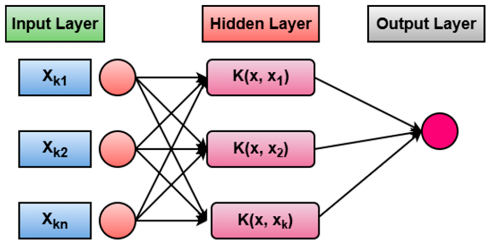
KELM is a novel machine learning method that combines extreme learning machines (ELM) with kernel methods. KELM is designed with only one hidden layer rather than many in a conventional neural network, and uses randomly assigned fixed input weights, making training much shorter [19]. The kernel function is a crucial part of the model that transforms the data into a higher-dimensional space, enabling KELM to learn complex patterns and relationships. This makes KELM a valuable tool for nonlinear regression and classification applications, such as photocatalysis, where it can be used to model and predict rate constants under different conditions. The network architecture of the kernel extreme learning machine is shown in Figure 13.

Equation (1) presents the best ELM single-hidden-layer feed-forward neural network architecture [20].

$$\mathrm{F}\left({\mathrm{x}}_{\mathrm{i}}\right)={\sum }_{\mathrm{i}=1}^{\mathrm{m}}{\mathsf{\beta }}_{\mathrm{i}}\mathrm{g}\left({\mathrm{w}}_{\mathrm{i}}\cdot {\mathrm{x}}_{\mathrm{i}}+{\mathrm{b}}_{\mathrm{i}}\right)={\mathrm{o}}_{\mathrm{i}}\hspace{1em}\left(\mathrm{i}=\mathrm{1,2},3,\dots ,\mathrm{N}\right)$$

(1)

where F(x_i) is the ith target value of the extreme learning machine, ${\beta }_i$ and w_i are the target weight vector and input weight vector of the ith neuron in the hidden and input layers, b_i is the bias, N is the number of samples, and m is the number of neurons in the hidden layer. Equation (2) represents the best ELM training phase.

$$||\mathrm{H}\left({\mathrm{w}}_1,\dots ,{\mathrm{w}}_{\mathrm{m}},{\mathrm{b}}_1,\dots ,{\mathrm{b}}_{\mathrm{m}}\right)\widehat{\mathrm{B}}-\mathrm{T}||=\underset{{\mathsf{\beta }}_{\mathrm{i}}}{\min }\left|\right|\mathrm{H}\left({\mathrm{w}}_1,\dots ,{\mathrm{w}}_{\mathrm{m}},{\mathrm{b}}_1,\dots ,{\mathrm{b}}_{\mathrm{m}}\right)\mathrm{B}-\mathrm{T}||$$

(2)

where T, H, and B are the target values, t_i is the ith output vector, h(x) is the feature mapping in the hidden layer, and n is the number of neurons in the output layer. Equation (3) represents the least squares solution of the output weight.

$$\widehat{\mathrm{B}}={\mathrm{H}}^{\mathrm{T}}{\left(\mathrm{H}{\mathrm{H}}^{\mathrm{T}}+\mathrm{C}\mathrm{I}\right)}^{-1}\mathrm{T}$$

(3)

where C and I are the penalty term and unit matrix. Equation (4) is the kernel function, and Equation (5) is a kernel function that influences the KELM model’s performance.

$${\mathsf{\Omega }}_{\mathrm{E}}=\mathrm{h}\left({\mathrm{x}}_{\mathrm{i}}\right)\hspace{0.17em}\mathrm{h}\left({\mathrm{x}}_{\mathrm{j}}\right)=\mathrm{K}\left({\mathrm{x}}_{\mathrm{i}},{\mathrm{x}}_{\mathrm{j}}\right)$$

(4)

$$\mathrm{K}\left(\mathrm{x},\mathrm{y}\right)\mathrm{ }=\mathrm{ }\exp \left(-\mathsf{\nu }|\mathrm{x}\mathrm{ }-\mathrm{ }\mathrm{y}{|}^2\right)$$

(5)

where v is the kernel width of radial basis function [21].

4.3.2. Crested Porcupine Optimizer–Support Vector Regression (CPO-SVR)

CPO–SVR is a hybrid machine learning method that combines the strengths of a powerful regression model with a metaheuristic optimization algorithm to achieve better predictive performance. SVR is commonly employed for nonlinear regression problems because of its strong generalization and ability to model complex relationships between input and output variables. The effectiveness of SVR, however, still largely depends on proper tuning of the hyperparameters, including the regularization parameter C, the kernel parameter γ, and the insensitive loss parameter ϵ [22]. To overcome this problem, the Crested Porcupine Optimizer (CPO), a nature-inspired metaheuristic optimization algorithm, is used to automatically find optimal parameter values. The CPO–SVR model can improve prediction accuracy and stability on complex engineering and environmental datasets, while reducing training error through the SVR regression function, retaining the advantages of CPO’s exploration and exploitation capabilities [23]. 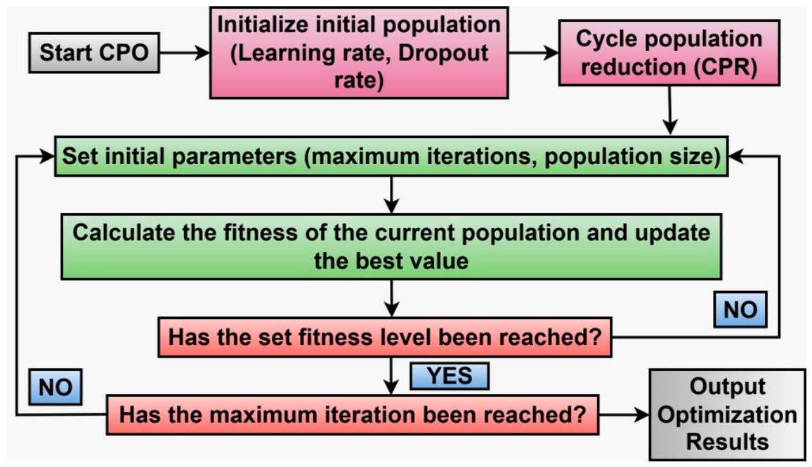Figure 14 presents the step-by-step presentation of CPO–SVR.

Equation (6) presents the standard notation for the SVR optimization problem [24].

$${\displaystyle \frac{1}{2}}|w{|}^2+C{\sum }_{i=1}^n\left({\mathsf{\xi }}_i+{\mathsf{\xi }}_i^{*}\right)$$

(6)

Equation (7) shows the SVR function.

$$\mathrm{f}\left(\mathrm{x}\right)={\sum }_{\mathrm{i}=1}^{\mathrm{n}}\left({\mathsf{\alpha }}_{\mathrm{i}}-{\mathsf{\alpha }}_{\mathrm{i}}^{\mathrm{*}}\right)\mathrm{K}\left({\mathrm{x}}_{\mathrm{i}},\mathrm{x}\right)+\mathrm{b}$$

(7)

Equation (8) displays the radial basis kernel function.

$$\mathrm{K}\left({\mathrm{x}}_{\mathrm{i}},{\mathrm{x}}_{\mathrm{j}}\right)=\exp \left(-\mathsf{\gamma }|{\mathrm{x}}_{\mathrm{i}}-{\mathrm{x}}_{\mathrm{j}}{|}^2\right)$$

(8)

The CPO position update is given by Equation (9).

$${\mathrm{X}}_{\mathrm{i}}^{\mathrm{t}+1}={\mathrm{X}}_{\mathrm{i}}^{\mathrm{t}}+{\mathrm{r}}_1\left({\mathrm{X}}_{\mathrm{b}\mathrm{e}\mathrm{s}\mathrm{t}}-{\mathrm{X}}_{\mathrm{i}}^{\mathrm{t}}\right)+{\mathrm{r}}_2\left({\mathrm{X}}_{\mathrm{j}}^{\mathrm{t}}-{\mathrm{X}}_{\mathrm{k}}^{\mathrm{t}}\right)$$

(9)

where x_i and x_j are the input feature vectors, y_i is the actual output value, f(x) is the regression function, K (x_i, x_j) is the kernel function, w is the weight vector, b is the bias term, C is the regularization parameter, $\gamma$ is the kernel parameter, ${\xi }_i+{\xi }_i^{*}$ are the slack variables, ${\alpha }_i-{\alpha }_i^{\mathrm{*}}$ are the Lagrange multipliers, $X_i^t$ is the candidate solution at iteration t, X_best is the best solution found so far, and r₁ and r₂ are the random numbers in [0, 1].

4.3.3. Harris Hawks Optimizer–Support Vector Regression (HHO-SVR)

HHO-SVR is a new nature-inspired metaheuristic algorithm inspired by the cooperative hunting strategy of Harris’s hawks. The algorithm mimics the dynamic combination of exploration and exploitation that these birds use to obtain their food, including surprise pounces and sleek chases, and can search the complex solution space efficiently [25]. HHO-SVR has been proven to be a very efficient algorithm for various optimization problems, such as parameter tuning in machine learning, feature selection, and engineering designs, owing to its high convergence, strong global search capability, and avoidance of local optima. It is a combination of exploration and exploitation, making it well-suited to solving nonlinear, high-dimensional, and constrained optimization problems. 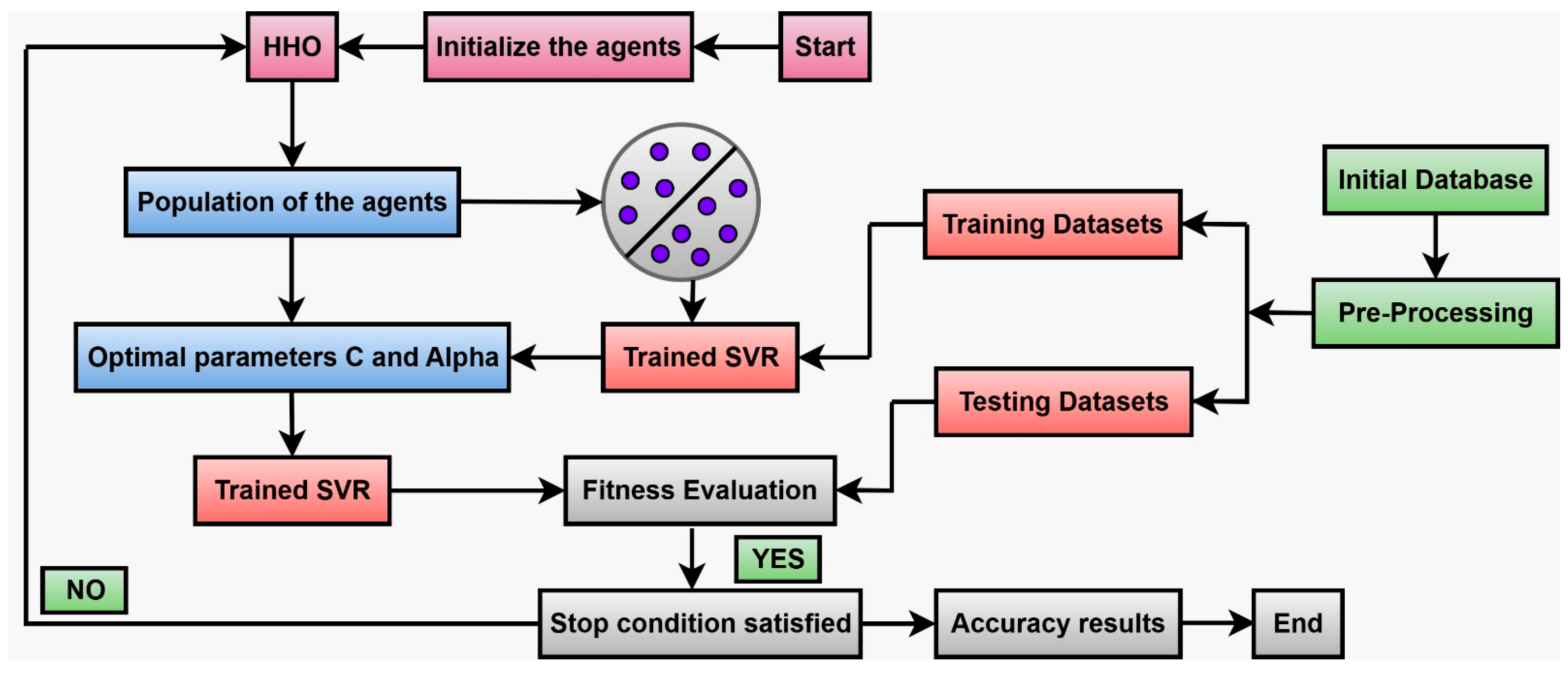Figure 15 presents the workflow details for the HHO-SVR metaheuristic algorithm [26].

Equations (10) and (11) are utilized for normal notation and optimal hyperparameter selections [27].

$$\mathrm{N}\mathrm{o}\mathrm{r}\mathrm{m}\mathrm{a}\mathrm{l} \mathrm{n}\mathrm{o}\mathrm{t}\mathrm{a}\mathrm{t}\mathrm{i}\mathrm{o}\mathrm{n} (\mathrm{A}\mathrm{t}\mathrm{t}\mathrm{a}\mathrm{c}\mathrm{k} \mathrm{P}\mathrm{h}\mathrm{a}\mathrm{s}\mathrm{e}) {\mathrm{X}}_{\mathrm{i}}^{\mathrm{t}+1}={\mathrm{X}}_{\mathrm{i}}^{\mathrm{t}}+{\mathrm{r}}_1\left({\mathrm{X}}_{\mathrm{b}\mathrm{e}\mathrm{s}\mathrm{t}}-{\mathrm{X}}_{\mathrm{i}}^{\mathrm{t}}\right)+{\mathrm{r}}_2\left({\mathrm{X}}_{\mathrm{j}}^{\mathrm{t}}-{\mathrm{X}}_{\mathrm{k}}^{\mathrm{t}}\right)$$

(10)

$$\mathrm{O}\mathrm{p}\mathrm{t}\mathrm{i}\mathrm{m}\mathrm{a}\mathrm{l} \mathrm{H}\mathrm{y}\mathrm{p}\mathrm{e}\mathrm{r}\mathrm{p}\mathrm{a}\mathrm{r}\mathrm{a}\mathrm{m}\mathrm{e}\mathrm{t}\mathrm{e}\mathrm{r}\mathrm{s} \mathrm{s}\mathrm{e}\mathrm{l}\mathrm{e}\mathrm{c}\mathrm{t}\mathrm{i}\mathrm{o}\mathrm{n} {\left(\mathrm{C},\mathsf{\gamma },\mathsf{ϵ}\right)}_{\mathrm{o}\mathrm{p}\mathrm{t}\mathrm{i}\mathrm{m}\mathrm{a}\mathrm{l}}=\arg \_\min \left(\mathrm{M}\mathrm{S}\mathrm{E}\right)$$

(11)

where $X_i^t$ = candidate solution at iteration t, X_best = best solution found by HHO, C = regularization parameter, and $ϵ$ = insensitive loss parameter in SVR.

4.3.4. Statistical Parameters for ML Model Analysis

Several widely accepted statistical validation indicators were used to validate the soft computing models developed, such as the coefficient of determination (R²), root mean square error (RMSE), mean absolute error (MAE), mean square error (MSE), Pearson correlation coefficient (PCC), Willmott index (WI), Nash–Sutcliffe efficiency (NSE), and Legates–McCabe index (LM). The coefficient of determination (R²) indicates the percentage of variance accounted for by the model, while RMSE, MAE, and MSE refer to the number of errors that occur in making predictions from the model—the lower the value, the better the model performs. PCC assesses the strength of the linear relationship between predicted and observed values. The Willmott index (WI) is a technique that improves the precision of relative RMSE and MSE by mitigating their insensitivity to outliers. It uses a refined version of MSE to minimize biasing errors. LM is another outlier-resistant alternative that uses absolute difference instead of squaring errors. NSE normalizes the error and is therefore a scale-independent statistical parameter. NSE ranges from 0 to 1, and the closer it is to 1, the more skillful the model is at predicting the data mean. The model’s absolute prediction errors and the spread of the observed data can be compared using the LM index, which provides an additional measure of the model’s accuracy. The statistical parameters provide a comprehensive assessment of the reliability, accuracy, robustness, and generalization performance of the models for predicting rate constant values for the photocatalytic reactions, and presented in Equations (12)–(18).

Coefficient of determination	${\mathrm{R}}^2=1-{\displaystyle \frac{{\sum }_{\mathrm{i}=1}^{\mathrm{n}}{\left({\mathrm{y}}_{\mathrm{i}}-\widehat{{\mathrm{y}}_{\mathrm{i}}}\right)}^2}{{\sum }_{\mathrm{i}=1}^{\mathrm{n}}{\left({\mathrm{y}}_{\mathrm{i}}-\overline{\mathrm{y}}\right)}^2}}$	(12)
Root mean square error	$\mathrm{R}\mathrm{M}\mathrm{S}\mathrm{E}=\sqrt{{\displaystyle \frac{1}{\mathrm{n}}}{\displaystyle \sum _{\mathrm{i}=1}^{\mathrm{n}}}{\left({\mathrm{y}}_{\mathrm{i}}-\widehat{{\mathrm{y}}_{\mathrm{i}}}\right)}^2}$	(13)
Mean absolute error	$\mathrm{M}\mathrm{A}\mathrm{E}={\displaystyle \frac{1}{\mathrm{n}}}{\displaystyle \sum _{\mathrm{i}=1}^{\mathrm{n}}}\left|{\mathrm{y}}_{\mathrm{i}}-\widehat{{\mathrm{y}}_{\mathrm{i}}}\right|$	(14)
Mean square error	$\mathrm{M}\mathrm{S}\mathrm{E}={\displaystyle \frac{1}{\mathrm{n}}}{\displaystyle \sum _{\mathrm{i}=1}^{\mathrm{n}}}{\left({\mathrm{y}}_{\mathrm{i}}-\widehat{{\mathrm{y}}_{\mathrm{i}}}\right)}^2$	(15)
Pearson coefficient correlation	$\mathrm{P}\mathrm{C}\mathrm{C}={\displaystyle \frac{{\sum }_{\mathrm{i}=1}^{\mathrm{n}}\left({\mathrm{y}}_{\mathrm{i}}-\overline{\mathrm{y}}\right)\left(\widehat{{\mathrm{y}}_{\mathrm{i}}}-\overline{\widehat{\mathrm{y}}}\right)}{\sqrt{{\sum }_{\mathrm{i}=1}^{\mathrm{n}}{\left({\mathrm{y}}_{\mathrm{i}}-\overline{\mathrm{y}}\right)}^2\sqrt{{\sum }_{\mathrm{i}=1}^{\mathrm{n}}{\left(\widehat{{\mathrm{y}}_{\mathrm{i}}}-\overline{\widehat{\mathrm{y}}}\right)}^2}}}}$	(16)
Willmott index	$\mathrm{W}\mathrm{I}=1-{\displaystyle \frac{{\sum }_{\mathrm{i}=1}^{\mathrm{n}}{\left({\mathrm{y}}_{\mathrm{i}}-\widehat{{\mathrm{y}}_{\mathrm{i}}}\right)}^2}{{\sum }_{\mathrm{i}=1}^{\mathrm{n}}{\left(\left|\widehat{{\mathrm{y}}_{\mathrm{i}}}-\overline{\mathrm{y}}\right|+\left|{\mathrm{y}}_{\mathrm{i}}-\overline{\mathrm{y}}\right|\right)}^2}}$	(17)
Legates–McCabe index	$\mathrm{L}\mathrm{M}=1-{\displaystyle \frac{{\sum }_{\mathrm{i}=1}^{\mathrm{n}}\left|{\mathrm{y}}_{\mathrm{i}}-\widehat{{\mathrm{y}}_{\mathrm{i}}}\right|}{{\sum }_{\mathrm{i}=1}^{\mathrm{n}}\left|{\mathrm{y}}_{\mathrm{i}}-\overline{\mathrm{y}}\right|}}$	(18)

where y_i = observed value, $\widehat{y_i}$ = predicted value, $\overline{y}$ = mean of observed value, and n = number of data samples.

5. Conclusions

Advanced soft computing techniques were successfully applied to predict the reaction rate constant for the degradation of benzoic acid in artificial UV-driven photocatalytic tubular reactors. Experimental results indicated that the flow rate, reactor diameter, and artificial UV rays were the most significant factors on photocatalytic performance. The rate constant obtained from the artificial UV rays and flow rates increased the degradation efficiency. However, smaller reactor diameters yielded better photocatalytic performance, whereas larger diameters were limited by the extent of light penetration and mass transfer. The developed models showed excellent predictive ability; among them, the model developed using HHO-SVR achieved the highest PCC values for the training and testing datasets, near-unity WI values, and the highest LM values, indicating the best fit between the predicted and experimental reaction rate constants. The CPO-SVR model also showed better predictive performance than the KELM model. The results suggest that optimization-assisted machine learning can successfully recover the complex nonlinear relationships involved in photocatalytic reactions.

The model interpretability was further improved by SHAP analysis, which highlighted the most important operating parameters that influence the reaction rate constant and quantified each parameter’s contribution to the model prediction. This explainable artificial intelligence framework yielded significant physical insights into the photocatalytic process and boosted trust in the developed models. The proposed methodology is, from a practical point of view, a reliable and computationally efficient design tool for photocatalytic treatment systems for reactors, process optimization, and operational control. The combination of soft computing, metaheuristics, and explainability offers a promising strategy for enhancing the design of intelligent photocatalytic reactors and sustainable water treatment technologies.

6. Future Recommendations

Future research should expand the experimental database to encompass a wider range of operating conditions, including different types of pollutants, photocatalysts, reactor geometries, light intensities, pH levels, and temperatures, to enhance model generalization and robustness. Additionally, the implementation of newer deep learning architectures, such as Long Short-Term Memory (LSTM), Gated Recurrent Unit (GRU), Transformer-based models, and hybrid physics-informed machine learning models, should be explored to improve prediction accuracy. In addition, coupling computational fluid dynamics (CFD) with artificial intelligence might also yield a better understanding of the coupled effects of hydrodynamics, mass transfer, and photon distribution on photocatalysis. Multi-objective optimization algorithms for degrading and minimizing energy consumption should also be explored for future studies. Furthermore, the combination of real-time monitoring systems, digital twins, and explainable artificial intelligence techniques would enable intelligent process control and industrial-scale deployment of photocatalytic reactors. Finally, validating the developed models in pilot- and full-scale treatment systems will be crucial for evaluating their applicability and scalability in sustainable water treatment operations.

References

- Xia, H.; Ahmad, M.A.; Guo, J.; Yang, Y. Unraveling the Roles of MW/UV/TiO2 Photocatalysis Technologies for Organic Wastewater Treatment. Catalysts 2023, 13, 754. [Google Scholar] [CrossRef]
- van Walsem, J.; Verbruggen, S.W.; Modde, B.; Lenaerts, S.; Denys, S. CFD investigation of a multi-tube photocatalytic reactor in non-steady-state conditions. Chem. Eng. J. 2016, 304, 808–816. [Google Scholar] [CrossRef]
- Amakiri, K.; Khan, M.M. Recent Advances in Photocatalytic Reactor Design and Process Optimization for Effluent Treatment. In Sustainable Effluent Treatment and Resource Recovery, Volume 2; ACS Symposium Series; American Chemical Society: Washington, DC, USA, 2025; Volume 1518, pp. 141–180. [Google Scholar] [CrossRef]
- Fang, Z.; Ma, L.; Duan, J.; Zhu, K.; Zhang, X.; Yang, Z. Flow Field Structure Optimization and Inlet Parameters in Tubular Photocatalytic Reactors: A CFD-Based Study. Catalysts 2025, 15, 798. [Google Scholar] [CrossRef]
- Bekele, T.; Alamnie, G. The photocatalytic degradation of organic pollutants-a comprehensive overview. Results Chem. 2025, 18, 102758. [Google Scholar] [CrossRef]
- Abdelfattah, I.; El-Shamy, A.M. A comparative study for optimizing photocatalytic activity of TiO2-based composites with ZrO2, ZnO, Ta2O5, SnO, Fe2O3, and CuO additives. Sci. Rep. 2024, 14, 27175. [Google Scholar] [CrossRef] [PubMed]
- Alhamdan, E.Z.; Spicer, D.; Cates, E.L. Factors affecting vacuum ultraviolet (185 nm) emission intensities in low-pressure mercury lamp photoreactors for photolytic destruction of water contaminants. J. Water Process Eng. 2025, 75, 107909. [Google Scholar] [CrossRef]
- Ildefonso-Ojeda, B.; Hernández-Chávez, M.; Álvarez-Lemus, M.A.; López-González, R.; Contreras-Bárbara, J.R.; Roa-Tort, K.; Rivera-Fernández, J.D.; Fabila-Bustos, D.A. Analysis and Application of UV-LED Photoreactors for Phenol Removal. Catalysts 2025, 15, 748. [Google Scholar] [CrossRef]
- Bloh, J.Z. A Holistic Approach to Model the Kinetics of Photocatalytic Reactions. Front. Chem. 2019, 7, 128. [Google Scholar] [CrossRef] [PubMed]
- Savage, T.; Basha, N.; McDonough, J.; Krassowski, J.; Matar, O.; del Rio Chanona, E.A. Machine learning-assisted discovery of flow reactor designs. Nat. Chem. Eng. 2024, 1, 522–531. [Google Scholar] [CrossRef]
- Solout, M.V.; Ghasemi, J.B. Predicting photodegradation rate constants of water pollutants on TiO2 using graph neural network and combined experimental-graph features. Sci. Rep. 2025, 15, 19156. [Google Scholar] [CrossRef] [PubMed]
- Na, I.; Kim, T.; Qiu, P.; Son, Y. Machine learning model to predict rate constants for sonochemical degradation of organic pollutants. Ultrason. Sonochemistry 2024, 110, 107032. [Google Scholar] [CrossRef] [PubMed]
- Xochihua Juan, J.L.; Solis Maldonado, C.; Luna Sánchez, R.A.; Enciso Díaz, O.J.; Rojas Ronquillo, M.R.; Sandoval-Rangel, L.; Pineda Aguilar, N.; Ramos Delgado, N.A.; Martínez-Vargas, D.X. TiO2 doped with europium (Eu): Synthesis, characterization and catalytic performance on pesticide degradation under solar irradiation. Catal. Today 2022, 394–396, 304–313. [Google Scholar] [CrossRef]
- Rehman, A.; Iqbal, M.A.; Haider, M.T.; Majeed, A. Artificial Intelligence-Guided Supervised Learning Models for Photocatalysis in Wastewater Treatment. AI 2025, 6, 258. [Google Scholar] [CrossRef]
- Javed, M.F.; Shahab, M.Z.; Asif, U.; Najeh, T.; Aslam, F.; Ali, M.; Khan, I. Evaluation of machine learning models for predicting TiO2 photocatalytic degradation of air contaminants. Sci. Rep. 2024, 14, 13688. [Google Scholar] [CrossRef] [PubMed]
- Javed, M.F.; Siddiq, B.; Onyelowe, K.; Khan, W.A.; Khan, M. Metaheuristic optimization algorithms-based prediction modeling for titanium dioxide-Assisted photocatalytic degradation of air contaminants. Results Eng. 2024, 23, 102637. [Google Scholar] [CrossRef]
- Patel, J.; Parmar, M.; Shahabuddin, S.; Tyagi, I.; Suhas; Gaur, R. Designing a Z-scheme rGO–SnS2 synergistic photocatalyst for photocatalytic mineralization of atrazine and 2,4-dichlorophenoxyacetic acid and applying machine learning for predictive modelling of photocatalytic performance. Nanoscale Adv. 2025, 7, 3485–3507. [Google Scholar] [CrossRef] [PubMed]
- Feroz, S.; Raut, N.; Al-Maimani, R. Utilization of solar energy in degrading organic pollutant-A case study. Int. J. Cond. Monit. Diagn. Eng. Manag. 2011, 14, 33–37. [Google Scholar]
- Li, C.; Zhou, J.; Dias, D.; Gui, Y. A Kernel Extreme Learning Machine-Grey Wolf Optimizer (KELM-GWO) Model to Predict Uniaxial Compressive Strength of Rock. Appl. Sci. 2022, 12, 8468. [Google Scholar] [CrossRef]
- Jamei, M.; Hasanipanah, M.; Karbasi, M.; Ahmadianfar, I.; Taherifar, S. Prediction of flyrock induced by mine blasting using a novel kernel-based extreme learning machine. J. Rock Mech. Geotech. Eng. 2021, 13, 1438–1451. [Google Scholar] [CrossRef]
- Roushangar, K.; Aghajani, N.; Ghasempour, R.; Alizadeh, F. The potential of ensemble WT-EEMD-kernel extreme learning machine techniques for prediction suspended sediment concentration in successive points of a river. J. Hydroinformatics 2021, 23, 655–670. [Google Scholar] [CrossRef]
- Chen, B.; Chen, Y.; Cao, L.; Chen, C.; Yue, Y. An Improved Crested Porcupine Optimization Algorithm Incorporating Butterfly Search and Triangular Walk Strategies. Biomimetics 2025, 10, 766. [Google Scholar] [CrossRef] [PubMed]
- Gao, Y.; Wang, J.; Yu, W.; Yi, L.; Guo, F. Crested Porcupine Optimizer-Optimized CNN-BiLSTM-Attention Model for Predicting Main Girder Temperature in Bridges. Appl. Sci. 2024, 14, 7356. [Google Scholar] [CrossRef]
- Su, X.; He, X.; Zhang, G.; Chen, Y.; Li, K. Research on SVR Water Quality Prediction Model Based on Improved Sparrow Search Algorithm. Comput. Intell. Neurosci. 2022, 2022, 7327072. [Google Scholar] [CrossRef] [PubMed]
- Qiao, H.; Zhang, M.; Bano, M. Harris Hawks Optimization for Soil Water Content Estimation in Ground-Penetrating Radar Waveform Inversion. Remote Sens. 2025, 17, 1436. [Google Scholar] [CrossRef]
- Houssein, E.H.; Mohamed, M.; Younis, E.M.G.; Mohamed, W.M. A hybrid Harris Hawks Optimization with Support Vector Regression for air quality forecasting. Sci. Rep. 2025, 15, 2275. [Google Scholar] [CrossRef] [PubMed]
- Khalifeh, S.; Akbarifard, S.; Khalifeh, V.; Zallaghi, E. Optimization of water distribution of network systems using the Harris Hawks optimization algorithm (Case study: Homashahr city). MethodsX 2020, 7, 100948. [Google Scholar] [CrossRef] [PubMed]
Figure 1.
Frequency distribution and sample density histogram of the dependent target variable (a) Length (b) Diameter (c) Flow rate, and (d) Rate Constant (the Y-axis (‘Count’) is the absolute number of experimental trials, and the X-axis is the absolute experimental value of the evaluated independent parameter).
Figure 2.
Prediction using KELM on training and test data set (Aa,Ba) comparison between predicted and actual target value (Ab,Bb) Absolute prediction error and (Ac,Bc) Error distribution. (‘Target’ represents the true, experimentally measured reaction rate values, ‘Output’ represents the predicted rate values mapped by the models).
Figure 3.
Prediction on the training dataset using HHO-SVR (a) comparison between predicted and actual target value (b) Absolute prediction error and (c) Error distribution. (‘Target’ represents the true experimentally measured reaction rate values, ‘Output’ represents the predicted rate values mapped by the model).
Figure 4.
Prediction on the testing dataset using HHO-SVR (a) comparison between predicted and actual target value (b) Absolute prediction error and (c) Error distribution. (‘Target’ represents the true, experimentally measured reaction rate values, ‘Output’ represents the predicted rate values mapped by the model).
Figure 5.
Prediction on the training dataset using CPO-SVR (a) comparison between predicted and actual target value (b) Absolute prediction error and (c) Error distribution. (‘Target’ represents the true, experimentally measured reaction rate values, ‘Output’ represents the predicted rate values mapped by the models).
Figure 6.
Prediction on the testing dataset using CPO-SVR (a) comparison between predicted and actual target value (b) Absolute prediction error and (c) Error distribution. (‘Target’ represents the true, experimentally measured reaction rate values, Output’ represents the predicted rate values mapped by the models).
Figure 7.
R2, RMSE, MAE, and MSE metric analyses.
Figure 8.
Comparison of PCC, WI, NSE, and LM for training and testing dataset.
Figure 9.
Training and testing dataset for actual vs predicted values.
Figure 10.
Convergence of SVR using HHO and CPO.
Figure 11.
SHAP analysis for the input and output variables.
Figure 12.
Experimental uncertainty analysis of the measured rate constant vs. diameter for different flow rates.
Figure 13.
Kernel extreme learning machine network architecture.
Figure 14.
The procedure workflow of CPO-SVR.
Figure 15.
Workflow for the HHO-SVR algorithm.