1. Introduction
How to reduce nitrogen oxide (NO
x) emissions from coal-fired power plants has become an important task of environmental treatment. Selective catalytic reduction denitration (SCR de-NO
x) technology is one of the mature flue gas denitration technologies [
1]. Many efforts have been made to optimize the SCR system, such as superior catalyst technology, enhanced de-NO
x control strategy, and byproduct limitation [
2]. However, it is very difficult to control the amount of NH
3 injection accurately. First, new energy is integrated into the power grid on a large scale in recent years. The boiler load needs to be changed to stabilize the fluctuation from the output power of new energy frequently. Therefore, the wide range of operating states poses certain difficulties in NH
3 injection control. Second, the upper limitation of NO
x emission is decreased to 50 mg/m
3 in China. In order to meet the national environmental standard, excessive NH
3 injection occurs easily. Hence, it is required to control NO
x emissions within the upper limitation and to avoid NH
3 escape. Third, the SCR de-NO
x system has large inertia, and it also has a large delay in NO
x analysis. When the operating state changes, the SCR system cannot adjust NH
3 injection in time based on the sampling inlet NO
x concentration, which can make the outlet NO
x emission deviate from the set value. Furthermore, the SCR de-NO
x process, which has the feature of nonlinear and multivariable coupling, is complex. When boiler load is stable, outlet NO
x emission can fluctuate widely for the reasons of flue gas temperature, flue gas flow rate, NH
3 injection and oxygen content. If boiler load changes, outlet NO
x emission changes dramatically. The proportion integration differentiation (PID) cascade control cannot achieve optimal control, which ensures high de-NO
x efficiency and low NH
3 escape. Therefore, the establishment of an accurate SCR model and the research of optimal control strategies are significant.
The current control strategy mainly uses a transfer function to control NH
3 injection. Considering the strong coupling between boiler parameter and SCR process parameter, the transfer function is difficult to reflect SCR de-NO
x process accurately. With the application of a plant-level supervisor information system, operating data can be viewed and recalled easily. Therefore, data-driven modeling and control methods are widely used. Data-driven modeling methods, such as Hammerstein–Wiener [
3], radial basis function autoregressive exogenous [
4], online support vector regression [
5], neural network, nonlinear autoregressive exogenous and polynomial fitting [
6], have been used to predict NO
x emission. Although most models are applied for diesel engines, the reaction principle is the same as the SCR de-NO
x system of a coal-fired power plant. The differences are that the boiler parameter affects outlet NO
x emissions, and the NO
x analyzer has a large lag in the coal-fired power plant. In addition, the advanced thermal management control strategies of catalysts have been developed to reduce emission concentrations [
7].
Variable selection and delay estimation are investigated to simple model structure and improve model accuracy. Mutual information (MI), which denotes statistical dependence between any two variables, is a measure of variable correlation [
8]. Therefore, it can express a linear and nonlinear correlation [
9]. In order to improve the model accuracy, Stanišić et al. [
10] used the MI method to select input variables. However, how to select an evaluation strategy and how to estimate the MI value accurately are two main difficulties in variable selection by the MI method. In their evaluation strategy, Battiti et al. proposed the mutual information feature selection (MIFS) method [
11], which got a good result. After this, Peng et al. [
12] and Fleuret [
13] proposed a different evaluation strategy. The above methods mainly use one-dimensional MI to evaluate the variable set. When there are redundant variables, the subset of the optimal variables cannot be obtained. The literature [
10] used a single evaluation function as an indicator, which often leads to an imbalance between the relevant variable and redundancy variables. Considering the large time-delay process, the effect of time-delay needs to be considered in variable selection. Ludwig et al. [
14] used the MI method to estimate the time-delay and got better results in a case. However, the method ignores the effect of variable dimension on the MI value. In general, output variable
y(
t) not only related to input variable
xi(
t) at time
t, but also related to historical input
xi(
t − 1),
xi(
t − 2), …,
xi(
t −
li) before time
t. Here,
li is defined as the historical data length of the input variable
xi. Therefore, it is necessary to determine the historical data length of each input variable when the time-delay is estimated.
Recently, adaptive nonlinear model predictive controllers, such as model-based predictive controller [
15], the generalized predictive controller [
16], dynamic matrix controller [
17], nonlinear autoregressive moving average with exogenous inputs (NARMAX) based predictive controller [
18], the neural network-based predictive controller [
19] and subspace predictive controller [
20], have been used to control the NH
3 injection and got better effect compared with the conventional PID controller. However, some models (e.g., [
15,
16]) involved high order nonlinear optimization, which is time-consuming and gets a local minimum rather than a global minimum easily. Not all of the operating states are covered in the NARMAX prediction model. The neural network prediction model is difficult to be predicted online, quickly and accurately. The input variable of the subspace predictive model only relates to NH
3 injection. Hence, it cannot reflect other variables that affect outlet NO
x emission correctly. In addition, the control effect is also affected by the constraints, such as the NH
3 valve opening and the increment of NH
3 valve opening, which are neglected in the above literature.
The objective of this paper is to model outlet NOx emissions under the different operating state, thereby to facilitate controller design. The kernel partial least squares (KPLS) model shows a good effect when it deals with the high dimensionality and colinearity data. In this paper, a dynamic KPLS model incorporated with variable selection and delay estimation is proposed. The k-nearest neighbor mutual information (KNN_MI) was used for delay estimation, and the effect of historical data lengths on KNN_MI was taken into account. Based on the results of delay estimation, a bidirectional search based on the change rate of KNN_MI (KNN_MI_CR) was used for variable selection. In order to improve model update accuracy, delay–time difference (DTD) update algorithm and feedback correction strategy are proposed. In order to take advantage of the existing controller, which has rapid response-ability to deal with disturbance signals, a parallel control structure that can identify the dynamic model online by using operation data is proposed. The existing conventional controller is used as the main controller. The NH3 injection compensator (NIC) combined with the outlet NOx emission model are used as correction controller, which can ensure the outlet NOx emission is stable near the set value. The principle of NIC is to eliminate the adverse effects of the large inertia of the SCR system and the lag of NOx analysis through feed-forward compensation to a certain extent.
The paper is organized as follows: In
Section 2, the SCR de-NO
x process and its control strategy are described. In
Section 3, the delay estimation and variable selection method are presented. The experimental results of the benchmark dataset for variable selection are presented in
Section 4. The field data experiment for the SCR de-NO
x process is investigated in
Section 5, and the predictive accuracy of the outlet NO
x emission model and the control effect of the proposed control strategy are analyzed. Finally, concluding remarks are given in
Section 6.
2. The SCR de-NOx Process and Its Control Strategy
2.1. The SCR de-NOx Process
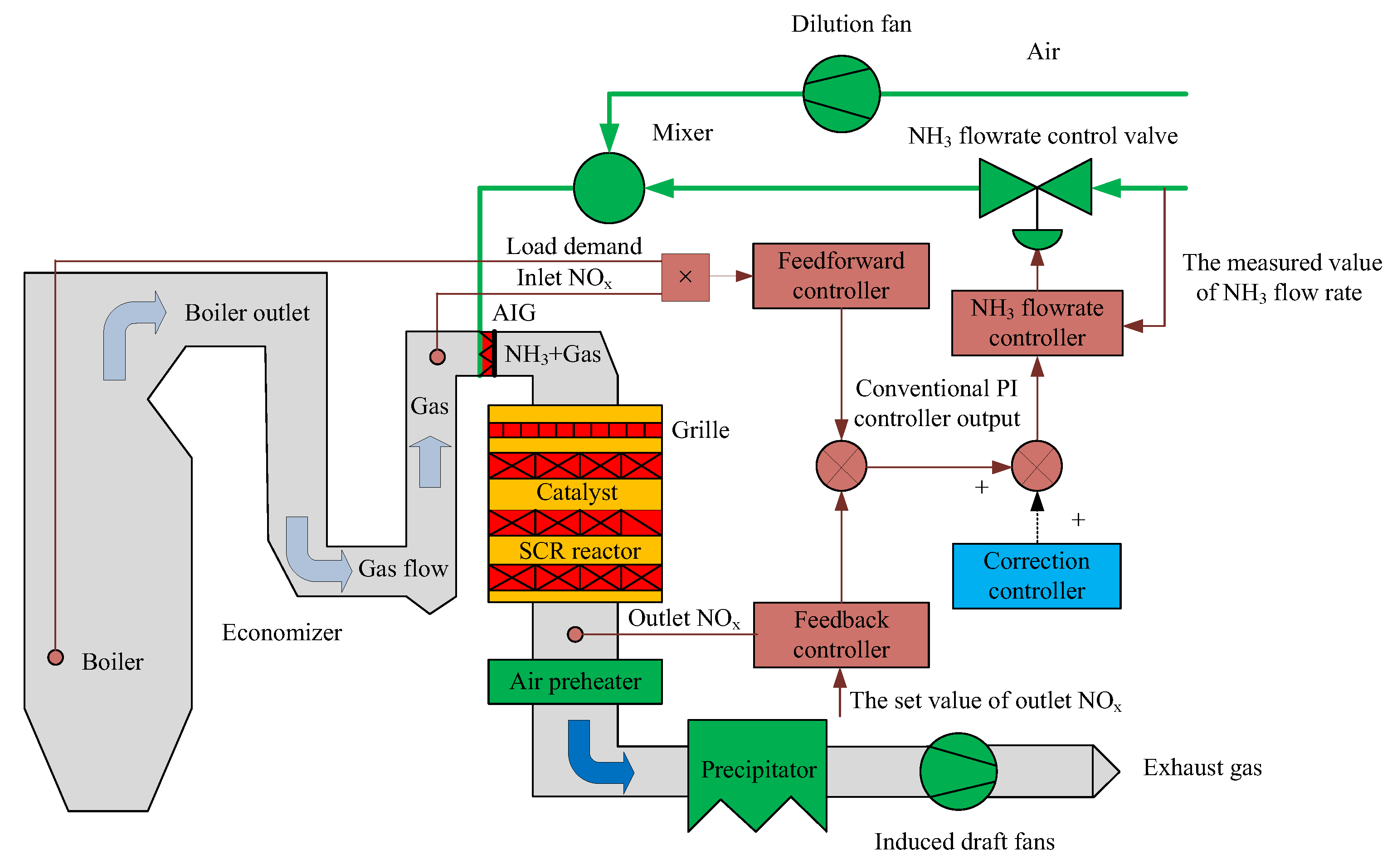
For a 1000 MW ultra-supercritical coal-fired power plant, the SCR de-NO
x system is shown in
Figure 1. The temperature of the SCR de-NO
x system is controlled by the bypass gas damper of the economizer in the upstream flue. Mixed with dilution air, the ammonia gas is sprayed by the NH
3 flow rate valve through the ammonia injection grid (AIG). In the reaction zone, the selective catalytic reaction occurs on the stainless steel plates, which are supported by the V
2O
5-WO
3-TiO
2 catalyst. Finally, the NO
x in the flue gas is converted into harmless N
2 and H
2O, and thereby the flue gas is purified. The main reaction of the SCR de-NO
x process is described as follows [
1]:
Actually, adverse side reaction will occur as follows [
1]:
It can be seen that the excessive NH3 injection leads to side reaction, and de-NOx efficiency is decreased because of the regeneration of NOx. Excess NH3 reacts with SO3 in the flue gas to form NH4HSO4 and (NH4)2SO4, which not only reduce the catalyst activity but also cause plugging and corrosion in the heated surface of the air preheater. In addition, increased NH3 escape could lead to secondary pollution. Secondary pollution refers to new pollutants, that is, unreacted ammonia gas.
2.2. The SCR de-NOx Process Control Strategy
Under the variable state of the power plant, the SCR de-NO
x process shows nonlinear, strong disturbance and large time-delay in NO
x analysis, so it is hard to achieve a good control effect by the existing PID control. Actually, except for controlling the temperature of the reaction zone by the bypass flue gas, it is necessary to design a better automatic control system which can control the NH
3 injection strictly. In order to ensure the most suitable NH
3/NO
x ratio, which is related to de-NO
x efficiency and ensure the NH
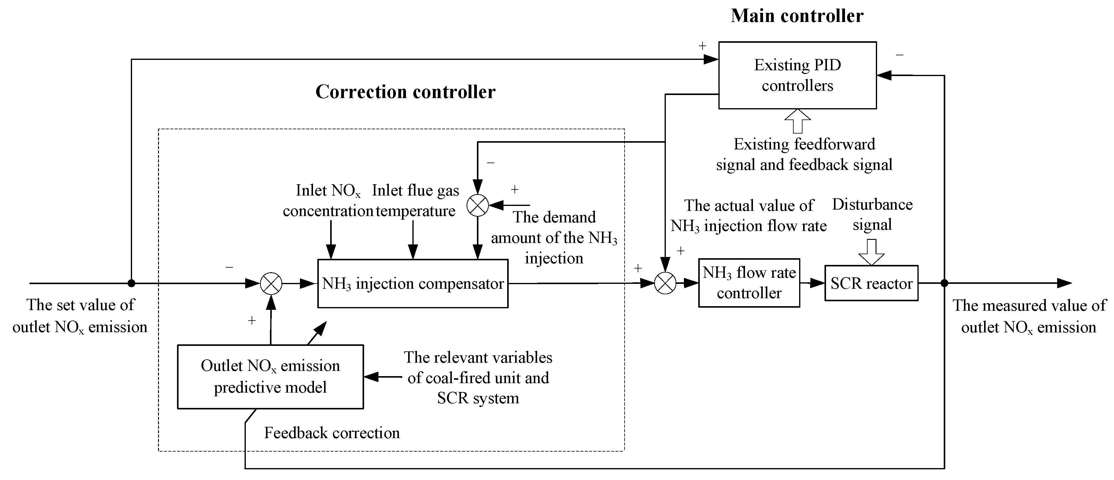
3 escape in a reasonable range, the proposed control system includes the main controller and the correction controller, which are in parallel operation. The main controller is the existing PID controller. The correction controller, which is shown in
Figure 1, is investigated in this paper. The parallel control system is shown in
Figure 2. The dynamic KPLS model is used as an outlet NO
x emission predictive model, which can be identified offline by the field data.
The correction controller includes three parts mainly: outlet NOx emission predictive model, feedback correction and NH3 injection compensator (NIC).
- (1)
Outlet NOx emission predictive model
In general, a dynamic data-driven model is constructed by adding the model input, such as the historical input data
and output data
. Therefore,
and
are selected as the new input variables in this paper. As a kind of model update method, the time difference (TD) algorithm can work out the variable drift and achieve better predictive accuracy. Moreover, the data model based on the TD algorithm does not need frequent reconstruction and parameter updating [
21]. The time-delay must be considered in the SCR deNO
x process. Hence, the delay-time difference (DTD) algorithm is proposed. Combining with the DTD method and KPLS model, the dynamic KPLS model, which is named DTD–KPLS, is proposed.
In general, the original input variable sample and output variable sample are used in the regression algorithm. However,
is calculated between the input variable
x(
t) at the time of
t and the input variable
x(
t −
i) at the time of
t − i through the TD method first. Similarly,
is calculated by the TD method:
Then, the relationship between
and
is modeled as:
If new data
is obtained, the TD of input data can be computed as:
Thus, the TD of output data can be predicted by the training model as:
Finally, the predicted output value at time
t′ is:
When the DTD method is used, the time-delay
needs to be considered in Equations (8) and (10). Hence, the training model becomes:
Hence, the actual predicted output is:
In this paper, the estimation of the DTD–KPLS model from the training set is depicted as follows [
22]:
The relevant variable samples are obtained, and the preprocessing, which contains outlier elimination and data filtering, is performed;
The input matrix Xreal and the output matrix are confirmed;
The time-delay of each input variable xi(I = 1,…,n) is estimated and the phase space reconstruction is made for Xreal. Hence, the new input variable matrix Xst is obtained;
The and of new input are calculated, and the of output is calculated;
The training set and are confirmed and and (z-score normalized) are obtained;
The kernel matrix
of the training set is calculated as:
The kernel matrix
of the training set is centered as:
Here, I is a unit matrix, 1n is a matrix whose all elements are 1 and whose dimension is n.
L is the number of latent variables, i iterates from 1 to L, and initialize the score vector of randomly.
The score vector
is calculated as:
The weight vector
is calculated as:
The score vector
is calculated as:
Step (8) to (11) is repeated until that is converged;
The matrix
and
are reduced as follows: until that
t and
u are extracted;
The regression coefficient
B is obtained, and the regression model of the training set is obtained as follows:
Here, T and U are both matrices, which are formed by score vector t and score vector u.
The prediction for the test set is similar to that for the training set, except the computation of the test kernel matrix
and the centralization of
:
Here, nt is the number of the test set. In addition, the kernel function uses the radial basis function (RBF) kernel in this paper.
- (2)
Feedback correction
In order to compensate for the prediction error, the feedback correction equation is as follows:
Here, is 0.3, is the corrected predicted value at time t, is the predicted value at time t, is the real value at time t.
Because the SCR de-NO
x process is very complicated, a complete mathematical model of the SCR process has still not been summarized. However, the compensation amount of NH
3 injection
can be calculated according to the nonlinear Equation (27):
is the demand amount of NH3 injection at the current operating state. is the NH3 injection flow rate at the time of t.
In this paper, the TD-KPLS model is used to establish the nonlinear model of the NIC, which is shown in Equation (27). The difference between the TD-KPLS model and DTD–KPLS model is that the samples of the TD-KPLS model are not reconstructed. In the model, the deviation between the corrected DTD–KPLS model output and the set value of outlet NOx mission is used as the input variables, and the compensation amount of NH3 injection is used as the output variable. In addition, input variables also include inlet flue gas temperature and inlet NOx concentration, which reflect the changing trend of the boiler load to a certain extent.
The adverse effects brought by the inertia characteristic of the SCR system are eliminated by feed-forward compensation. Hence, the NIC can compensate for the NH3 injection in time to ensure that the outlet NOx emission is stable at the set value.
In the SCR de-NOx system, the NH3 injection valve can be seen as a linear part, so the algorithm design and parameter setting are performed on the basis of that. However, the NH3 injection valve has a certain dead zone and saturation zone, which shows nonlinearity. Therefore, in this paper, the middle curve in the on and off stroke is taken as the fitting curve between the NH3 injection valve opening and the NH3 injection flow rate.
In order to avoid valve saturation and action frequently, the following constraints of the NH
3 injection valve need to be considered:
Here, UVmax and UVmin are the upper and lower limits for the NH3 valve opening. uVmax and uVmin are the upper and lower limits for the increment of the NH3 valve opening. represents the increment of the NH3 valve opening from the next time t+1 to the current time t.
5. The Field Data Experiment for SCR de-NOx Process
5.1. Field Data and Preselected Input Variables
The inlet NOx concentration and NH3 injection flow rate reflect the NH3/NOx molar ratio, which influences the de-NOx efficiency and the NH3 escape directly. The NH3 injection flow rate is controlled to match up the change of boiler load by the NH3 valve. Inlet O2 content influences outlet NOx concentration and de-NOx efficiency directly. Moreover, the change in boiler load often influences the inlet flue gas flow rate. Then, the flue gas temperature is changed through heat exchange. The inlet flue gas temperature influences the reaction rate and catalyst activity.
In a word, the outlet NO
x emission is related to many factors. In addition, the changes in boiler load, coal quality, and combustion condition could cause a large fluctuation in inlet NO
x concentration. Therefore, preselected input variables and the output variable are shown in
Table 4.
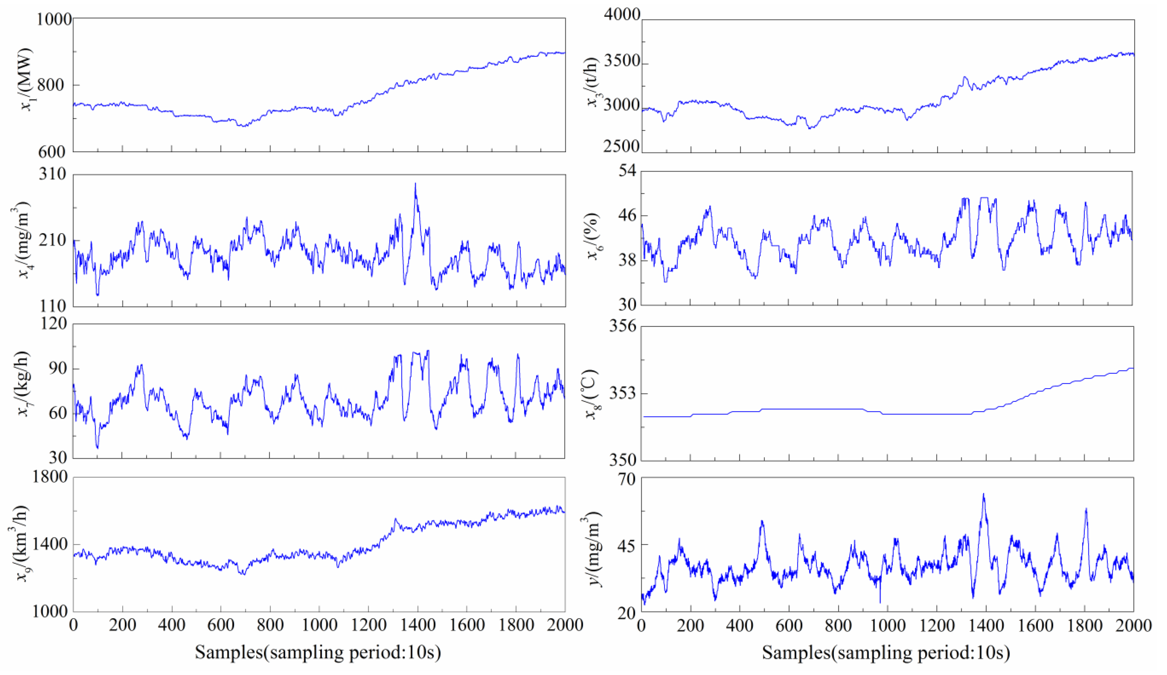
Assuming that coal quality is invariable, the selected field data cover steady state and variable state. One-dimensional linear interpolation is carried out on the measured NO
x concentration at the process of blowback. Therefore, 2000 samples were collected, and the sampling period is 10 s. Due to the length of this paper, the samples of part preselected input variables and output variables are shown in
Figure 6.
5.2. Result Analysis of Delay Estimation and Variable Selection
In general, the maximum time-delay of SCR reaction which includes NO
x analysis is 120~400 s, and the maximum time-delay of boiler load which influences inlet NO
x concentration is 600 s, so the range of τ is (20,60) from
x1 to
x3, and (1,40) from
x4 to
x9. T
max in Equation (32) is 1200 s, so the range of
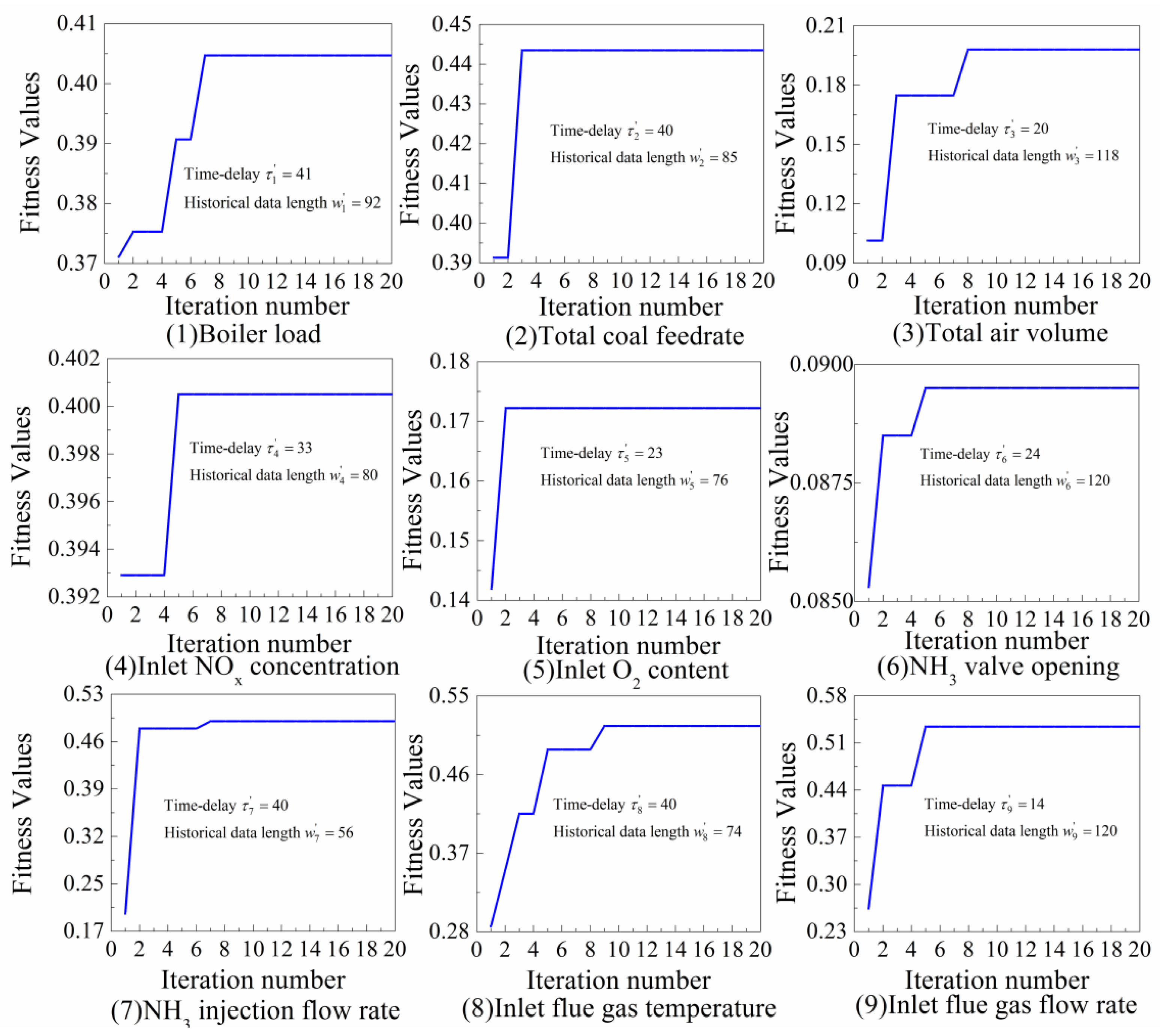
w is (1,120). The time-delay of each input variable is different-in-different operation point. The samples from 200 point to 500 point at 800 MW operating state are taken as an example to analyze the delay estimation and variable selection methods. The size of the SCR reactor is 11.67 m × 13.95 m × 12.6 m. The optimal fitness curves of the PSO algorithm for all preselected input variables are shown in
Figure 7, and the results are shown in
Table 5.
It can be seen from
Figure 7, each preselected variable reaches the optimal global solution before the 10th iteration, and the optimal parameter
and
are obtained. The optimal result multiplies the sampling period to obtain the time-delay of the preselected variable, which is shown in
Table 5.
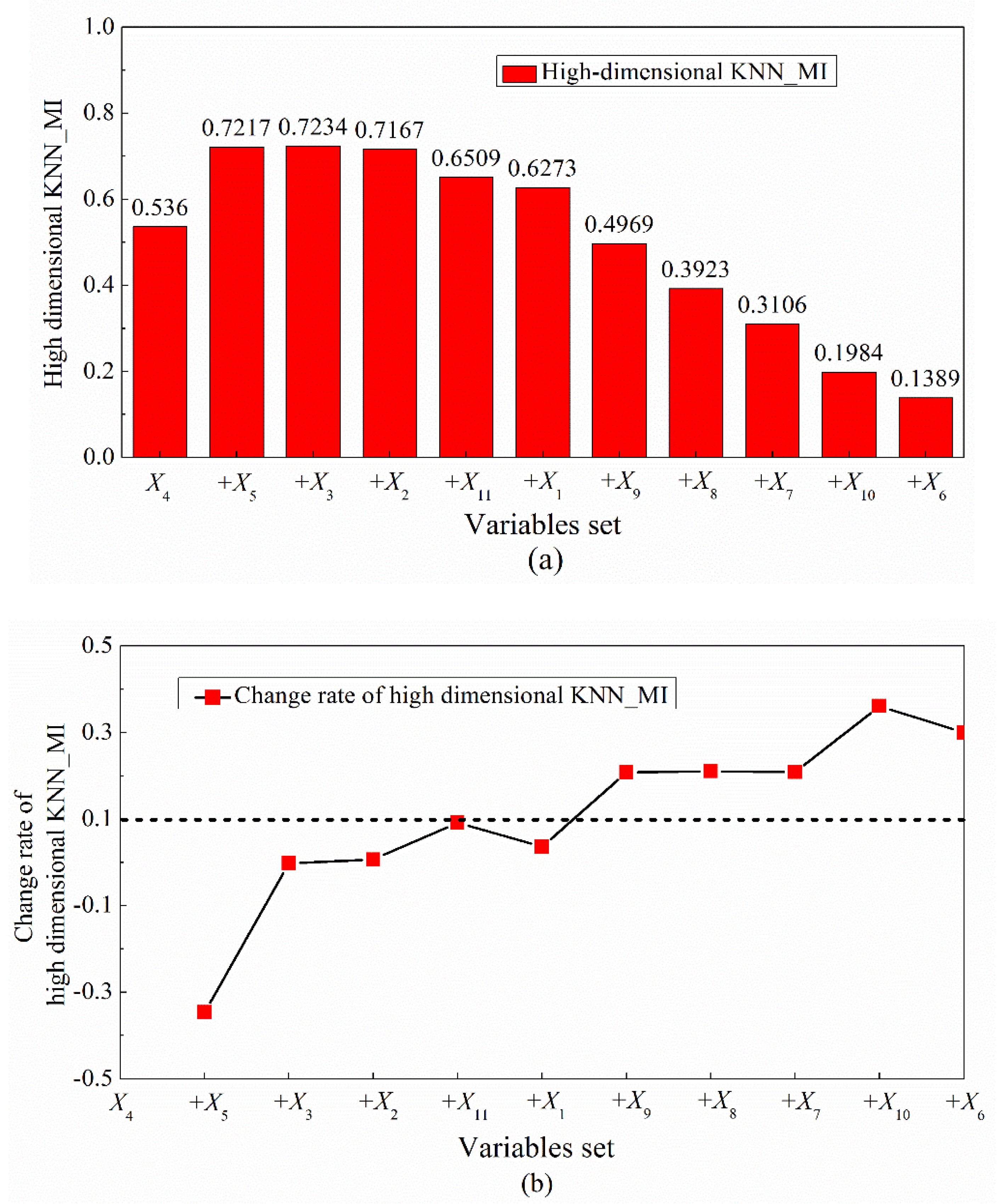
The effect of time-delay needs to be considered for the variable selection in SCR de-NOx process. Therefore, based on the delay estimation result, the phase space reconstruction on each input variable is performed first, and then the KNN_MI_CR method is used to select a suitable variable.
It can be seen from
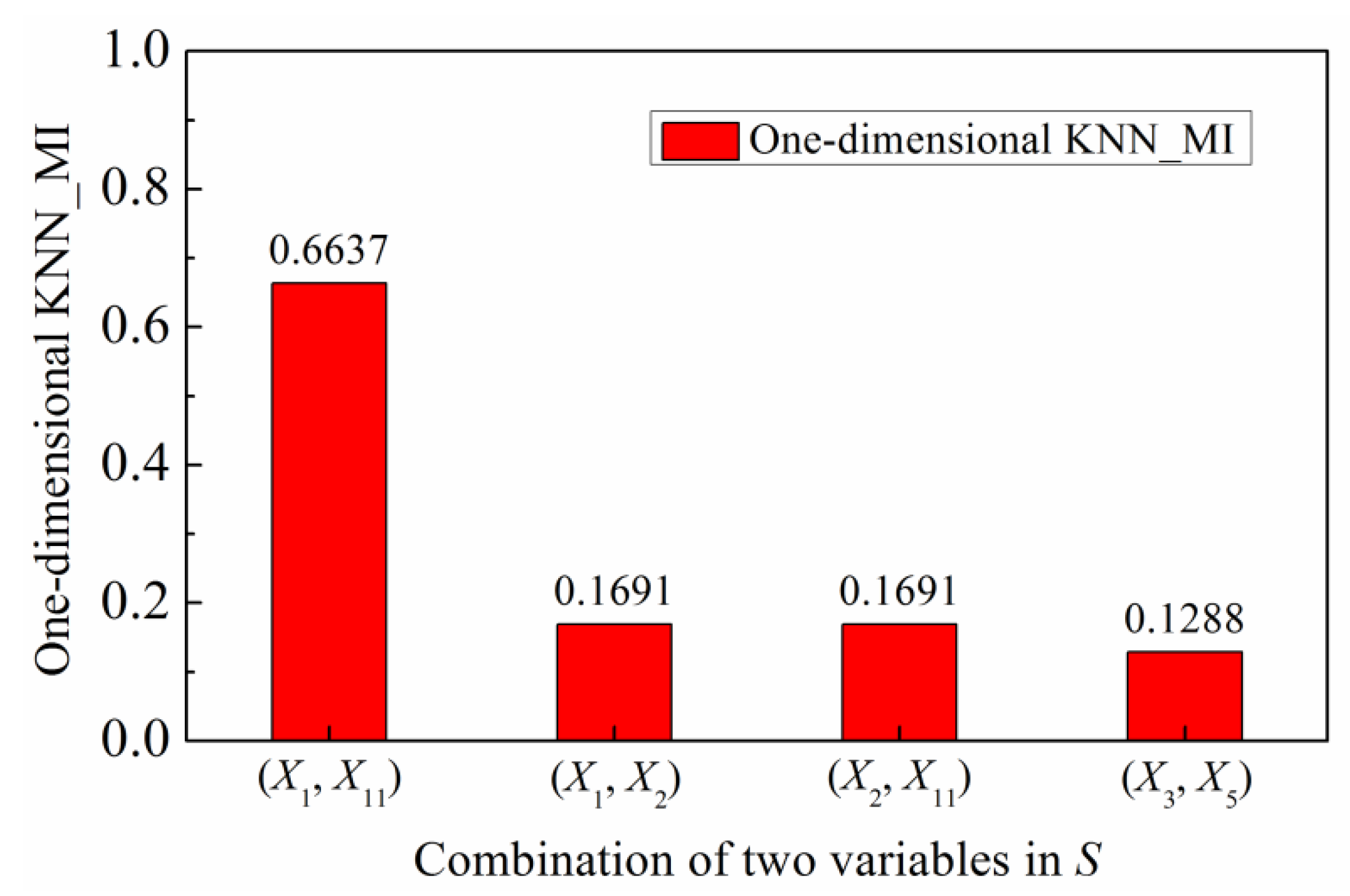
Table 6 that if the model samples are reconstructed by phase space, the result of variable selection is different. The DTD–KPLS model, whose variables are selected by the KNN_MI_CR method, has the highest predictive accuracy. Although the variable selection result is the same, the predictive accuracy of the DTD–KPLS model whose samples are reconstructed is improved in the BIF and CMIM method. In addition, the sequence of the selected input variable is different, and the model accuracy is different, which indicates that the consideration of high-dimensional KNN_MI is conducive to the selection of suitable input variables.
5.3. Analysis of Dynamic Model
In general, dynamic modeling is realized by adding the historical input data
and output data
as a new input of the model. The 2000 prediction samples are used to analyze model accuracy by using different input variables. The results are shown in
Table 7.
It can be seen from
Table 7 when input variables are
,
and
, the predictive accuracy of the model is highest. In addition, because the model input is historical input data before the current time
t, the DTD–KPLS model can predict the current value of the output variable in advance accurately.
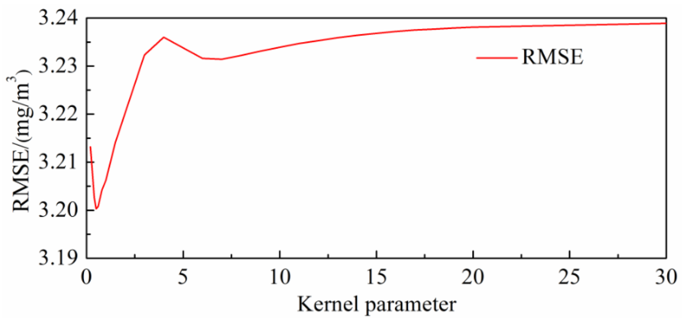
When parameter optimization is used in model control strategies, a large number of calculations need to be avoided. In this paper, the DTD–KPLS model has only one RBF kernel parameter. The predictive accuracy of the DTD–KPLS model in different kernel parameters is analyzed. The results are shown in
Figure 8.
The change rate of the RMSE value was no more than 1%, as shown in
Figure 8, which indicates that the predictive accuracy was not sensitive to the kernel parameter. Therefore, the DTD–KPLS model could adopt fixed parameters to avoid a large number of calculations in parameter optimization. In this paper, the single-step prediction time was 1 s, so it could meet the demand for control.
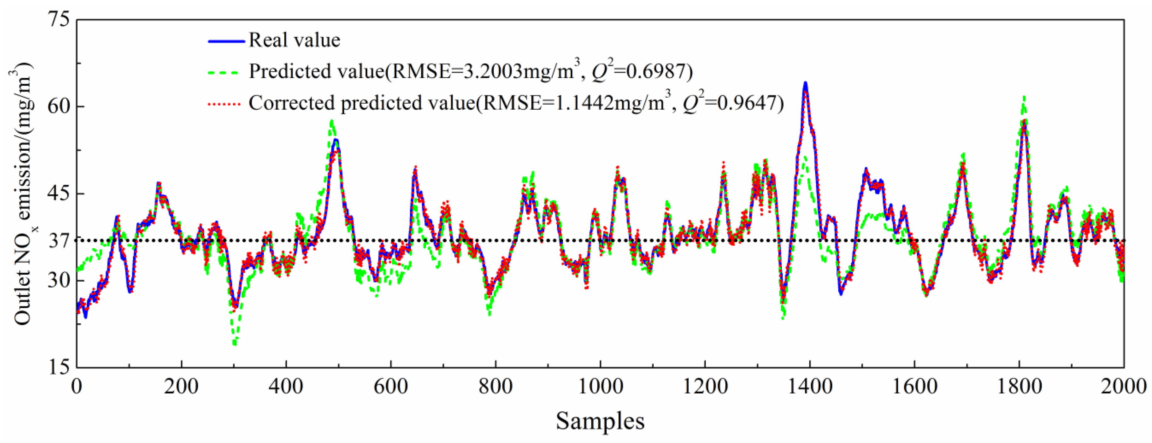
In order to compensate for the prediction error, this paper proposes a feedback correction strategy for the DTD–KPLS model. The predicted value and the corrected predicted value are shown in
Figure 9.
It can be seen from
Figure 9, and the DTD–KPLS model shows high predictive accuracy with a low RMSE of 3.2933 mg/m
3 and a high determinate coefficient (Q
2) of 0.7011 in the whole state. A large amount of NO
x was produced in a variable state. Hence the predictive accuracy was lower at the peak of the outlet NO
x emission curve. After feedback correction, the predicted values were closer to the real value. Steady state and variable state were covered in the model samples, so the DTD–KPLS model had strong self-adaptability.
5.4. Analysis of Control Effect
Two kinds of NH3 injection control modes have mainly existed in China. One is fixed NH3/NOx molar ratio control, and the other one is fixed outlet NOx value control. In this paper, the fixed outlet NOx value control was analyzed. First, the NOx flow rate was determined by the inlet NOx concentration and the flue gas flow rate, and the preset molar ratio was calculated. Then, the NH3/NOx molar ratio was corrected based on the measured value and the set value of outlet NOx emission. The amount of NH3 injection was determined by the corrected NH3/NOx molar ratio and the calculated NOx flow rate. Finally, the fixed outlet NOx emission was achieved.
In order to obtain the demand amount of NH
3 injection
at the current operating state, the transfer function from the NH
3 injection to the decreased amount of outlet NO
x emission was investigated through a dynamic characteristic test as follows:
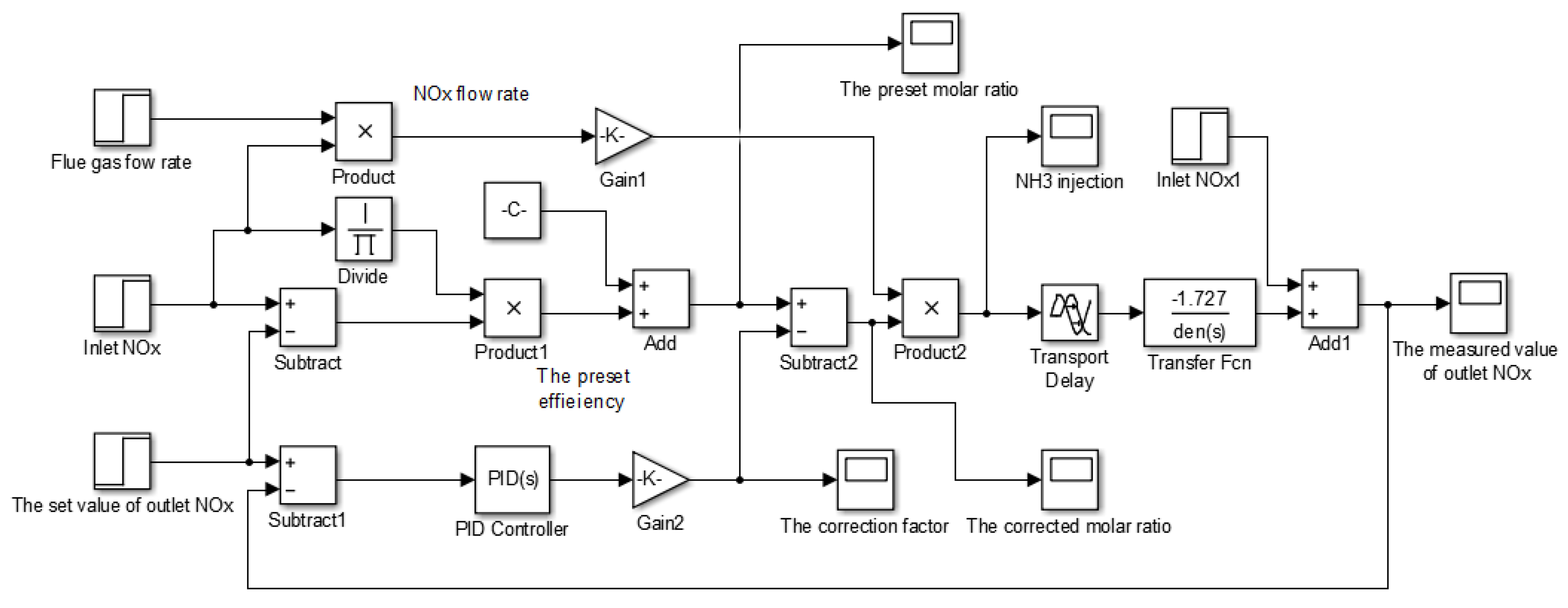
Then, the control structure diagram set up in MATLAB/SIMULINK is shown in
Figure 10.
In the field data in
Figure 6, the inlet NO
x and the flue gas flow rate fluctuated from 135~230 mg/m
3 to 120~160 km
3/h. During the simulation, the inlet NO
x, the flue gas flow rate and the set value of outlet NO
x were set to 160 mg/m
3, 1300 km
3/h and 37 mg/m
3, which were consistent with the field data. PID tuning program was used to get optimal PID parameters. The results are shown in
Figure 11,
Figure 12 and
Figure 13.
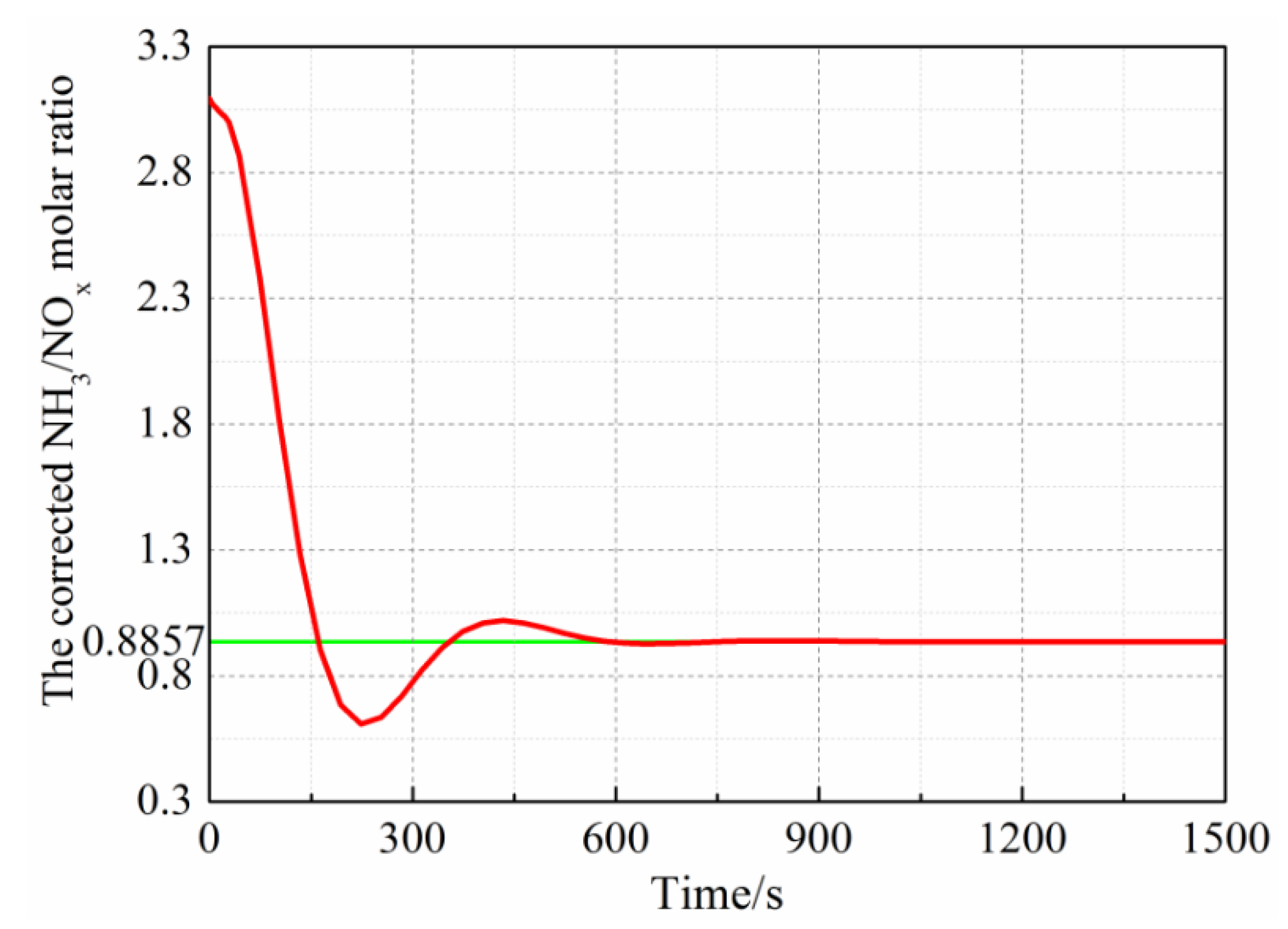
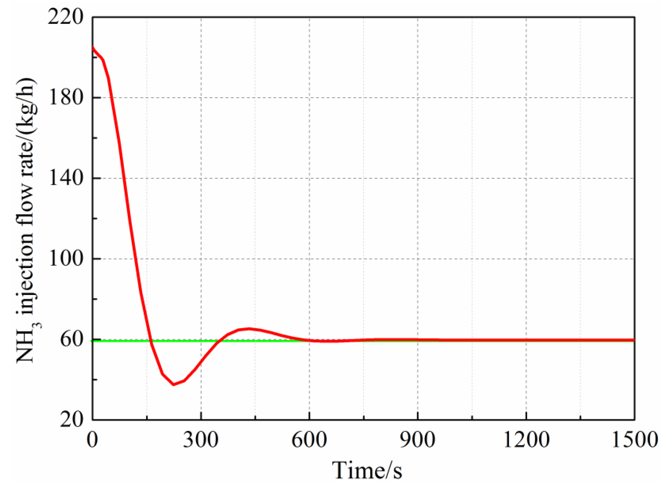
If the inlet NOx value and the set value of outlet NOx were fixed, as the deviation between them decreased, the PID controller reduced the actual NH3/NOx molar ratio; thereby, the amount of NH3 injection was reduced gradually. After the system was stabilized, the outlet NOx emission, the NH3 injection flow rate and the NH3/NOx molar ratio were stable at 37 mg/m3(set value), 60 kg/h and 0.8857, which were close to the average value of field data. So the demand amount of NH3 injection corresponding to the set value of outlet NOx emission was 59.6 kg/h, and this method could accurately simulate the fixed outlet NOx control mode. The control process lasted for nearly 1000 s before the system became stable. Hence, the existing system could not meet real-time control because of the long adjustment time.
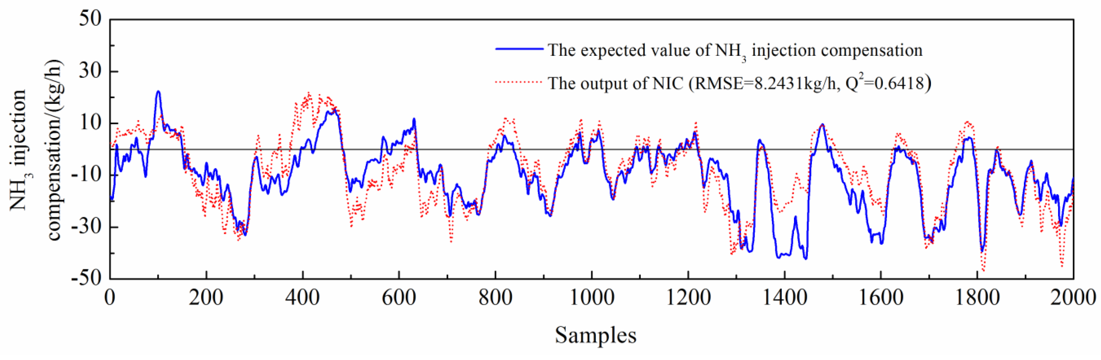
The predicted value of the TD-KPLS model was taken as the output of NIC in each model update. The input variables included the deviation between the corrected predicted NO
x emission value and the set value of outlet NO
x emission, inlet flue gas temperature and inlet NO
x concentration. The output variable was the amount of NH
3 injection compensation. The output of the NIC is shown in
Figure 14.
Figure 14 shows that the output of the NIC was consistent with the trend of the expected value of NH
3 injection compensation. Therefore, the predictive accuracy of TD-KPLS was high. In addition, the predicted value was a mostly negative value indicating that the amount of NH
3 injection was reduced by 11% after adding the NIC. Assuming that the price of NH
3 water was about 3000 RMB per ton, the data used in this paper was taken as an example. After the application of the NIC, the cost of de-NO
x could be saved by 531.2 RMB per day.
Because the SCR de-NO
x system had large inertia and had a large delay in NO
x analysis; hence, the following analysis started from the 100th point. The control effect of outlet NO
x emission is shown in
Figure 15.
Figure 15 shows the control effect of the existing controller was not ideal, and the outlet NO
x emission produced drastic fluctuation when the load changes. For example, the outlet NO
x emission exceeded the national NO
x emission standard (50 mg/m
3) at the 500, 1400 and 1800 points. In contrast, after the NIC was added, the outlet NO
x emission whose fluctuation ranged in ±5 mg/m
3 was stable near the set value. Therefore, the outlet NO
x emission was far lower than the national NO
x emission standard.
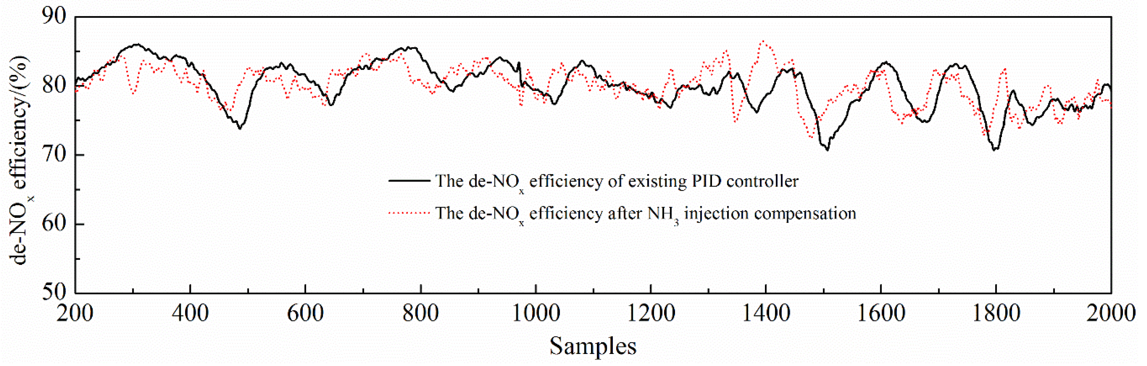
It can be seen from
Figure 16 that the minimum value of the de-NO
x efficiency after adding the NIC (76.31%) was higher than the minimum value of the de-NO
x efficiency of the existing controller (73.79%). The average de-NO
x efficiency was 80.12% by using the existing controller, and the average de-NO
x efficiency was 80.15% after adding the NIC. This indicated that the de-NO
x efficiency was basically unchanged after adding the NIC.
In order to calculate the NH
3 escape further, the following formula was introduced.
Here, t represents the sampling time; Wm is the measured NH3 injection flow rate, kg/h; Wc is the NH3 injection consumption, kg/h; Vgas is the inlet flue gas flow rate, m3/h; p is the NH3 escape, μg/m3.
Because the compensation amount of NH
3 injection in this paper was negative value mostly, the consumption of NH
3 injection was regarded unchanged basically.
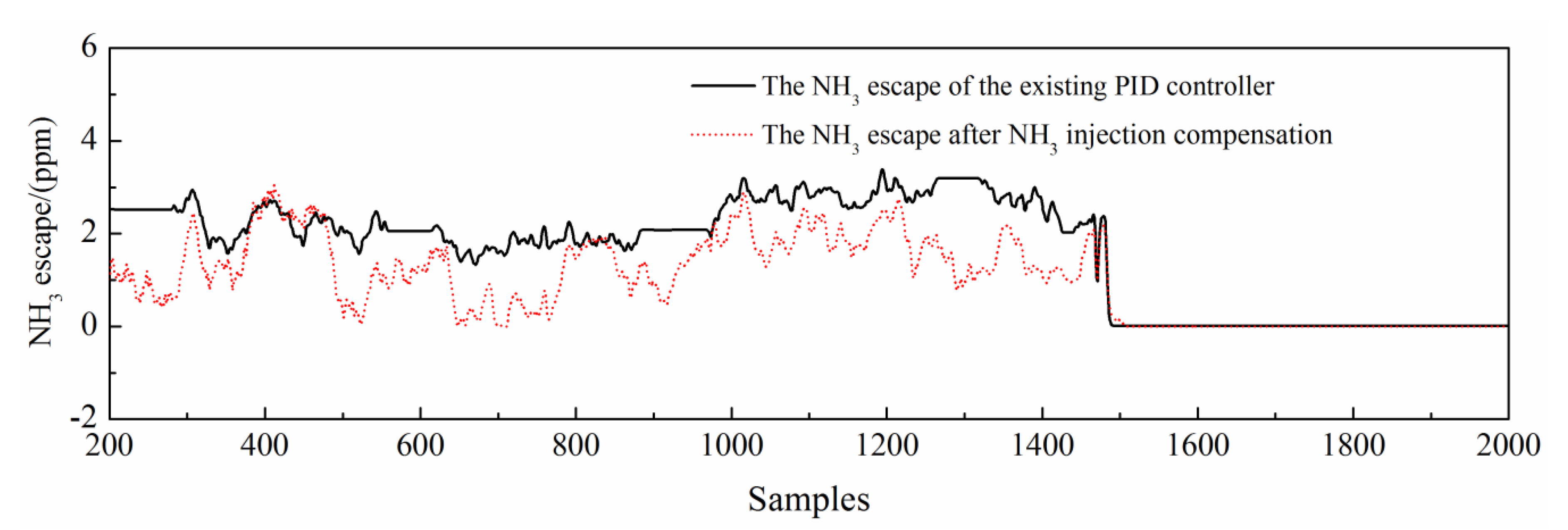
Figure 17 was the comparison between the NH
3 escape of the existing controller and the NH
3 escape after NH
3 injection compensation.
In
Figure 17, after the NIC was added, although the average of de-NO
x efficiency did not change, the NH
3 escape was reduced by 39% after NH
3 injection compensation.
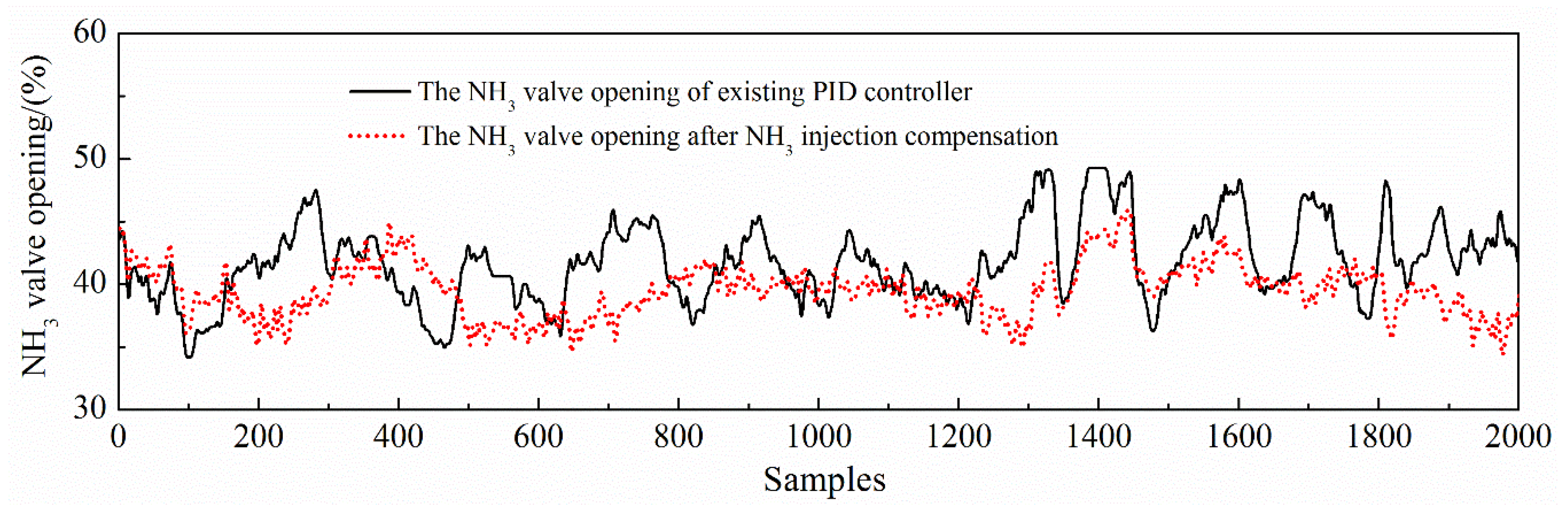
Actually, in order to avoid actuator saturation, the NH
3 injection valve opening was restrained by conditions (23) and (24) in the NH
3 injection control. The NH
3 valve opening of the existing controller and NH
3 valve opening after NH
3 injection compensation are shown in
Figure 18.
Due to the lag of NO
x analysis, the NH
3 control valve was prevented from being over-opened or over-closed. Therefore, when the NH
3 control valve was in automatic mode, the NH
3 valve opening was limited from
UVmin = 20% to
UVmax = 50%. In
Figure 18, the NH
3 valve opening of the existing controller reached 50% from 1300 points to 1500 points, which indicated that the actuator reached saturation in automatic control. When the NIC was used, the average of the NH
3 valve opening was reduced, thereby actuator saturation was avoided.
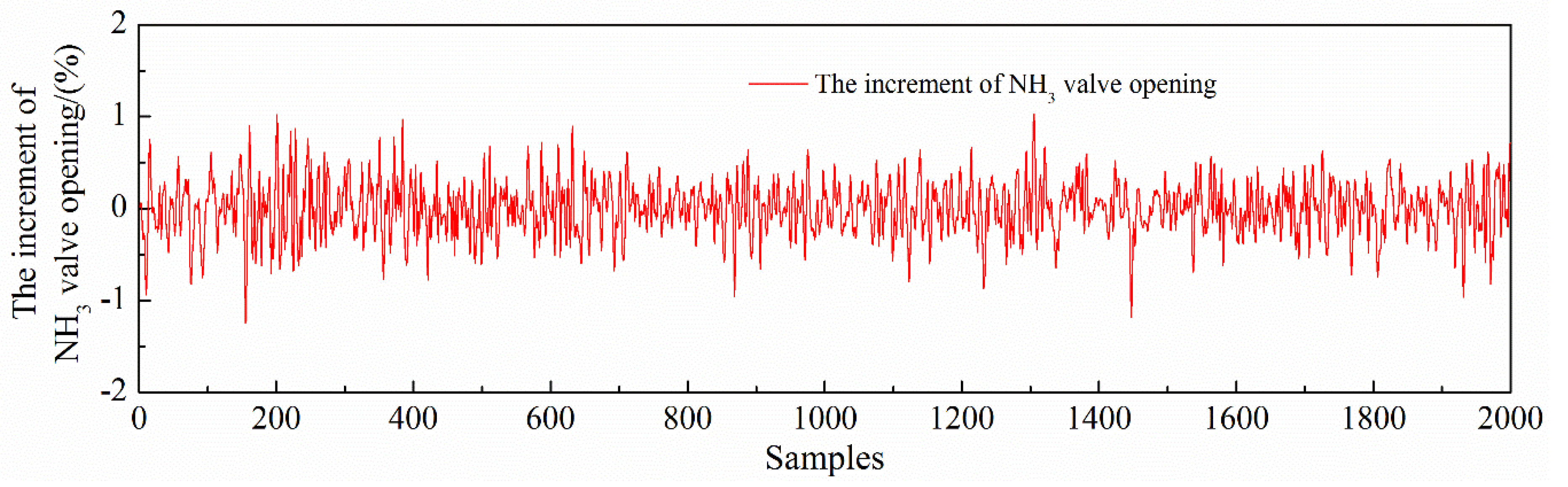
The upper limitation
uVmax and the lower limitation
uVmin of the increment of NH
3 valve opening were 2% and −2%, respectively.
Figure 19 shows that the increment of NH
3 valve opening after NH
3 injection compensation was within limitation. Therefore, the NH
3 valve was protected, and the control accuracy was improved.
In all, the proposed control strategy had a good control effect. Through the NH3 injection was adjusted by NIC continually, the controller could decrease the NH3 injection and decrease the NH3 escape as much as possible while ensuring that the high de-NOx efficiency and NOx emission meets the national NOx emission standard. Therefore, the operation cost was reduced, and secondary pollution caused by the incomplete reaction of NH3 was avoided.


