1. Introduction
The research question of this paper is whether a non-transparent distribution of power in a bargaining situation affects individuals differently depending on their gender. This is a relevant angle in view of complex real-world negotiations. Moreover, we are, to the best of our knowledge, the first to study gender effects in the multilateral bargaining game by Baron and Ferejohn [
1].
Gender differences in bargaining behavior and outcomes have, to date, almost exclusively been studied in the context of bilateral bargaining. This seems natural, as a central issue of economics, wage formation, is frequently characterized by bilateral situations, either in the form of negotiations between a labor union and an employer or as bargaining between an individual employee and his or her supervisor.
However, bargaining is also central to distributing resources in contexts where more than two agents are involved and agents have different power. For example, consider a small company with five shareholders, who have ownership shares of 26%, 23%, 20%, 17%, and 14%, and whose Articles of Association stipulate that more than 50% of the ownership interests must be behind a decision. Treating the percentage ownership shares as votes, this could be represented by the weighted voting game (51; 26,23,20,17,14), where 51 is the threshold that needs to be reached to pass a decision.
Voting weights do not always reflect individuals’ actual bargaining power in a transparent way. Due to the combinatorial nature of weighted voting, decision rules that look very different can be strategically equivalent, i.e., they result in exactly the same possibilities to form winning coalitions. In the weighted voting game presented above, the five shareholders are in fact symmetric, as any three of them can form a winning coalition. Generally, each weighted voting rule has an infinite number of representations, and we call two decision-making rules equivalent if they generate identical sets of winning and losing coalitions and thus imply the same real power. We refer to any differences between two representations that do not alter the sets of winning and losing coalitions as nominal. The voting game above is equivalent to (3; 1,1,1,1,1), which describes the distribution of power in the company in a more transparent way.
Non-transparent decision rules can have several reasons. Sometimes voting weights have been designed to conceal underlying power relations as was allegedly the case with the voting arrangements of the International Monetary Fund (see [
2]). In other cases, misalignment between voting weights and actual power seems to be rather due to negligence; the Council of the European Economic Community between 1958 and 1973 is a famous example [
3]. From a game-theoretic perspective, purely nominal differences in voting weights should not matter. If they are nevertheless found to influence behavior and outcomes, this indicates the presence of a “power illusion”, a possibility that has previously been studied in the context of structured multilateral bargaining [
4,
5,
6] and in unstructured bargaining [
7,
8]. Guerci et al. [
9] focuses on how experimental subjects learn about nominal weights, without a bargaining context.
Among the studies that considered nominal power differences in Baron–Ferejohn bargaining, evidence for power illusion is mixed. While [
5] found power illusion effects to apply only to inexperienced subjects [
4] (hereafter: MPT) reported that nominal differences can continue to influence agents’ behavior in spite of experience. In [
6], the effect of nominal weights is a secondary aspect, as main interest is to test the effect of adding a new player to a weighted voting game. Still, their experiment included a treatment with nominal power differences, which found that nominally strong players earned more than nominally weak players, but the difference was not significant. Overall, these results suggest that transparency of voting rules is desirable in the sense that the distribution of voting weights should reflect the intended distribution of actual power as much as possible. The case for transparency becomes even stronger when it turns out that the mere appearance of a bargaining situation leads to systematic differences in outcomes between women and men.
To answer our research question, we use data from the MPT experiment. In that experiment, a group of five persons divided a budget according to the rules of the multilateral bargaining game of [
1]. The decision rule in all treatments gave ex ante equal real bargaining power to all players. MPT contrasted a treatment where players’ symmetry was transparent with two ‘power illusion’ treatments that involved nominally different, non-transparent representations of the decision rule. In the present work, we first analyze whether the strategies adopted as proposer or responder differed systematically by gender in situations where influence was transparent (the
Base treatment). We then compare behavior in the transparent setting to behavior in a non-transparent situation, where all group members had nominally different weights and could be subject to ‘power illusion’ (the
Pit treatment). We document several behavioral differences between women and men in the absence of nominal differences. In particular, we find that women in the role of proposer claim less for themselves and also offer less to potential coalition partners than men. Women generally seek to form larger coalitions, whereas men more often form minimum winning coalitions. As a result, women earn less than men; this difference is basically unchanged by nominal weights.
Various empirical studies on wage negotiations such as, e.g., [
10], show that women request and receive lower salaries compared to men. Moreover, when it is unclear whether negotiations are possible, women are less likely than men to initiate salary negotiations [
11,
12]. These findings largely explain the difference in negotiation outcomes [
13] and point to the mechanisms behind the well-documented gender gap in wages [
14]. Experimental studies have looked at the factors underlying the behavioral differences in bargaining, e.g., attitudes to norm compliance [
13]. However, the existing body of experimental research has almost exclusively focused on bilateral bargaining situations, such as the ultimatum game [
15,
16] or two-player alternating offers bargaining [
17,
18].
An exception is Baranski et al. [
19] who analyze how the gender composition of a committee affects the outcomes of majoritarian bargaining. In their experiment, groups of three players split a budget according to a free-form bargaining protocol with costly delay. Their evidence shows that grand coalitions—i.e., including all group members—are more often formed in predominantly female groups, whereas minimal winning coalitions are more common the larger the proportion of male group members. With respect to bargaining behavior, [
19] found that men are more likely than women to make the initial offer and, when left out from a proto-coalition, men are more active in making offers to find partners (see [
20]).
Our findings confirm Baranski et al.’s result that female proposers are generally more inclined than male proposers to form grand coalitions. We also agree that this inclination is probably due to women’s greater prosociality. The most important difference between the two studies is that MPT was not specifically designed to investigate gender effects, but the effect of nominal power differences. In particular, subjects in MPT did not know the gender of the other agents in the bargaining situation. Therefore, the data do not allow us to analyze group composition and gender pairing effects, which are the main focus of [
19]. As a consequence, we cannot observe whether women are more likely to reject an offer if it comes from a male proposer, or whether the offers men make towards other men differ from those towards women. However, our data allow us to isolate behavioral differences between men and women when acting as proposer or responder, leaving gender pairing effects aside. Other differences between MPT and [
19] concern group size and the bargaining protocol. With regard to the latter, Tremewan and Vanberg [
21] have shown that the final divisions in structured and unstructured bargaining situations can be quite similar despite the different procedures.
The remainder of the paper is organized as follows:
Section 2 reviews our original experiment.
Section 3 presents our results regarding the interaction of gender and power illusion effects in bargaining.
Section 4 concludes. We provide additional materials in three appendices.
2. Multilateral Bargaining with Nominal Power Asymmetry
2.1. Experimental Design and Treatments
The MPT experiment implemented a closed rule Baron–Ferejohn game with five players and simple majority rule. The five group members decided how to split a fixed budget of 150 Tokens according to the following rules: At first, a proposer was selected randomly with equal recognition probabilities. Next, the proposer suggested an allocation to the other players, subject to not exceeding the total budget constraint. Then players simultaneously voted yes or no, and the proposal was accepted if at least three of the five players voted in favor; in that case, the game ended and the agreed allocation was implemented. If the proposal failed, then a new proposer was selected at random with the process being repeated until an allocation was passed. In the closed rule version of the Baron–Ferejohn game, it is not possible to amend the proposal, but a new round must be started with a new proposal.
The canonical representation of the group’s voting rule is R = (3; 1,1,1,1,1), i.e., each agent has one vote, and three votes are the threshold that needs to be met or exceeded to pass a proposal. R served as a baseline in the experiment, as it reflects the real bargaining power of the players in a particularly transparent way. As an equivalent, but non-transparent representation of the same voting rule, we focused on = (18; 9,8,7,6,5), which has the smallest integer weights such that the weights of all five players differ. Using a between-subjects design, we exposed subjects to either representation R or , referred to as the Base treatment and the Pit treatment, respectively. The latter was labeled PIT2 in MPT as the original experiment also included a third treatment condition (PIT1) using representation (7; 3,3,3,2,2). In the present paper, we aim to focus on the behavior of proposers and responders by gender with and without nominal power differences. However, the PIT1 treatment potentially involves either homophily or some kind of groupiness (social identity) between members of the same weight type (weight-2 vs. weight-3). These effects could also differ by gender and would then interact with the behavioral differences we are interested in here. We therefore chose not to use that treatment in the present study.
To avoid confounding factors, MPT considered the game without discounting, i.e., the budget to be divided did not shrink from round to round. The outcome associated with the unique subgame perfect equilibrium in stationary strategies—the common benchmark prediction—then is that the proposer allocates of the budget to herself and offers the continuation value of to each of two other agents. The two remaining agents are left out of this minimal winning coalition and receive zero payoffs. The proposal is approved without delay. Clearly, these theoretical predictions apply regardless of whether voting rules R or is presented to the players.
Each session in the MPT experiment consisted of 20 bargaining periods, which were either played consecutively or with a short break of ten minutes after the first 10 periods. The relevant experimental treatments are summarized in
Table 1; in total, 200 subjects participated. As can be seen from the sample breakdown in
Table A1 in
Appendix A, the sample was not gender-balanced, with a female share of 61%. Subjects were randomly rematched into groups between periods, but not between the rounds within a given bargaining game, and had no possibility to learn others’ gender or other characteristics. At the beginning of each period, each subject was randomly assigned her voting weight for that period (see [
8] for a methodological discussion of random vs. fixed roles).
After learning her own voting weight as well as the voting weights of the other four group members and the quota each player was prompted to enter a proposal on how to allocate the 150 Tokens. One of the five first-round proposals was randomly chosen (with equal probabilities), displayed to all group members and then voted upon. If the proposal obtained a simple majority, the proposed distribution was agreed and the period concluded. If the proposal failed, a new round of the same game was initiated, where one player—possibly the same as before—was randomly selected (with probability
) to make a proposal. This was repeated until an allocation was agreed upon, at which point subjects were informed of their individual payoff during that period. At the end of a session, one period from the first ten periods and from the last ten periods, respectively, was randomly chosen for payment. For further details regarding the experimental procedures, we refer to MPT. The instructions are provided in
Appendix B.
2.2. Results and Discussion
Comparing Base and Pit, our earlier study (MPT) demonstrated a number of power illusion effects in inexperienced players with respect to outcomes and behavior. In particular, inexperienced players’ payoffs and the proposer claims were strongly aligned with nominal weights. Similarly, the offers made to others were larger the larger the respondent’s nominal weight. Experience often but not always led to the attenuation or disappearance of these effects, making results in Pit more similar to those in Base. However, nominal weights continued to influence offering behavior for experienced players, but now larger offers were made to nominally less powerful responders. Comparing treatments with uninterrupted play over 20 bargaining situations and treatments with a break after the first 10 situations, MPT found significantly greater persistence of power illusion in the uninterrupted treatments, suggesting that the break enhanced subjects’ learning about the ‘real’ game. Overall, 63% of all coalitions were minimal; while less than predicted by theory, this share is similar to other experiments on Baron–Ferejohn bargaining. We found only very little variation across the different treatments, i.e., nominal weighting did not affect coalition size.
In our current analysis, we pool treatments with and without a short break, as also indicated in
Table 1. The reason for this is that we found the effect of the break to be independent of gender. However, we include a dummy in all regressions below to control for an observation coming from a “break” or a “no-break” condition.
Another difference of our analysis here compared to MPT concerns how we define inexperienced and experienced subjects. In MPT, we referred to observations from periods 1–5 as “inexperienced” and to those from periods 16–20 as “experienced”. By contrast, in the present analysis, we take the first ten periods to be “inexperienced” and refer to the last ten periods as “experienced”. The reason is that our experimental design had each player become a proposer twice within the first or last 10 periods. Therefore, if we chose only five periods, as in MPT, it would be possible that the same person was a proposer either zero, one or two times. This would be problematic, given that women and men behave differently.
2.3. Conjectures about Gender Effects
In the present paper, we are interested in whether the introduction of nominal voting weights affects female and male players’ behavior and payoffs differently. We first draw on the previous literature on gender effects in bilateral bargaining (e.g., [
15,
19]) to formulate hypotheses about gender specific bargaining behavior and outcomes. Second, a growing body of literature shows that there are gender differences with respect to overconfidence (e.g., [
22,
23]) and motivated reasoning (e.g., [
24]), finding specifically that men tend to be more overconfident and more prone to motivated reasoning about their performance. Our conjectures about gender effects of nominal weighting are based on the expectation that nominally greater power will increase individual tendencies toward overconfidence and motivated reasoning.
Hypothesis 1 (
H1)
. Earnings
- (a)
Men earn more than women.
- (b)
Nominal differences reinforce this.
The latter conjecture assumes the following behavior in the role as proposer:
Hypothesis 2 (
H2)
. Proposers
- (a)
The share that a male proposer allocates to himself is greater than the share that a female proposer allocates to herself.
- (b)
Nominal differences reinforce this.
The multilateral bargaining model suggests that players will base their decision on whether to accept or reject a proposal solely on the amount offered to them. In particular, they should accept any offer that at least corresponds to their continuation value. Alternatively, individuals’ minimal acceptable offer might be influenced by nominal weights.
Hypothesis 3 (
H3)
. Responders
- (a)
Women accept lower offers than men.
- (b)
A player’s acceptance threshold is higher the larger her or his weight.
- (c)
Responders’ probability to accept an offer depends negatively on the share demanded by the proposer.
The literature generally finds women to be more egalitarian than men (e.g., [
25,
26]). In our context of multilateral bargaining, egalitarianism has two elements, first the inclusiveness of the proposed coalition and second the proposed distribution of payoffs within the coalition. We thus suggest
Hypothesis 4 (
H4)
. Coalitions
- (a)
Female proposers are more inclusive than male proposers, i.e., they choose larger coalitions.
- (b)
Female proposers propose more equal distributions among the coalition members.
3. Results
We first present our experimental results regarding players’ payoffs (Hypothesis 1) and then turn to players’ behavior following the structure of Hypotheses 2–4 above. In
Section 3.5, we additionally address the question whether female proposers were motivated by risk aversion. Throughout, we focus on results from the first ten and the last ten periods, in order to distinguish clearly between inexperienced and experienced behavior.
Results in
Section 3.1 (payoffs) are based on the final round of each bargaining period.
Section 3.2 (proposer behavior) relies on players’ first round proposals in each bargaining period. Responder voting behavior is analyzed in
Section 3.3 using “yes” and “no” votes from all rounds of a bargaining period. Coalition formation (
Section 3.4) is investigated using first round proposals. Throughout the analyses, we assume that each individual first round proposal, each individual final round payoff, and each vote from all rounds of a bargaining period is an independent observation. To minimize repeated game effects, subjects were randomly rematched into groups between periods. Moreover, at the end of a session, only two periods were randomly chosen, respectively, from the first ten periods and from the last ten periods, to be paid off in private (random lottery incentive system, see [
27]). Altogether, we have
first round proposals and final round payoffs, respectively, per treatment. As bargaining took up to eight periods at maximum, we have (coincidentally) 2136 “yes” and “no” votes, both in
Base and
Pit.
1 3.1. Payoffs
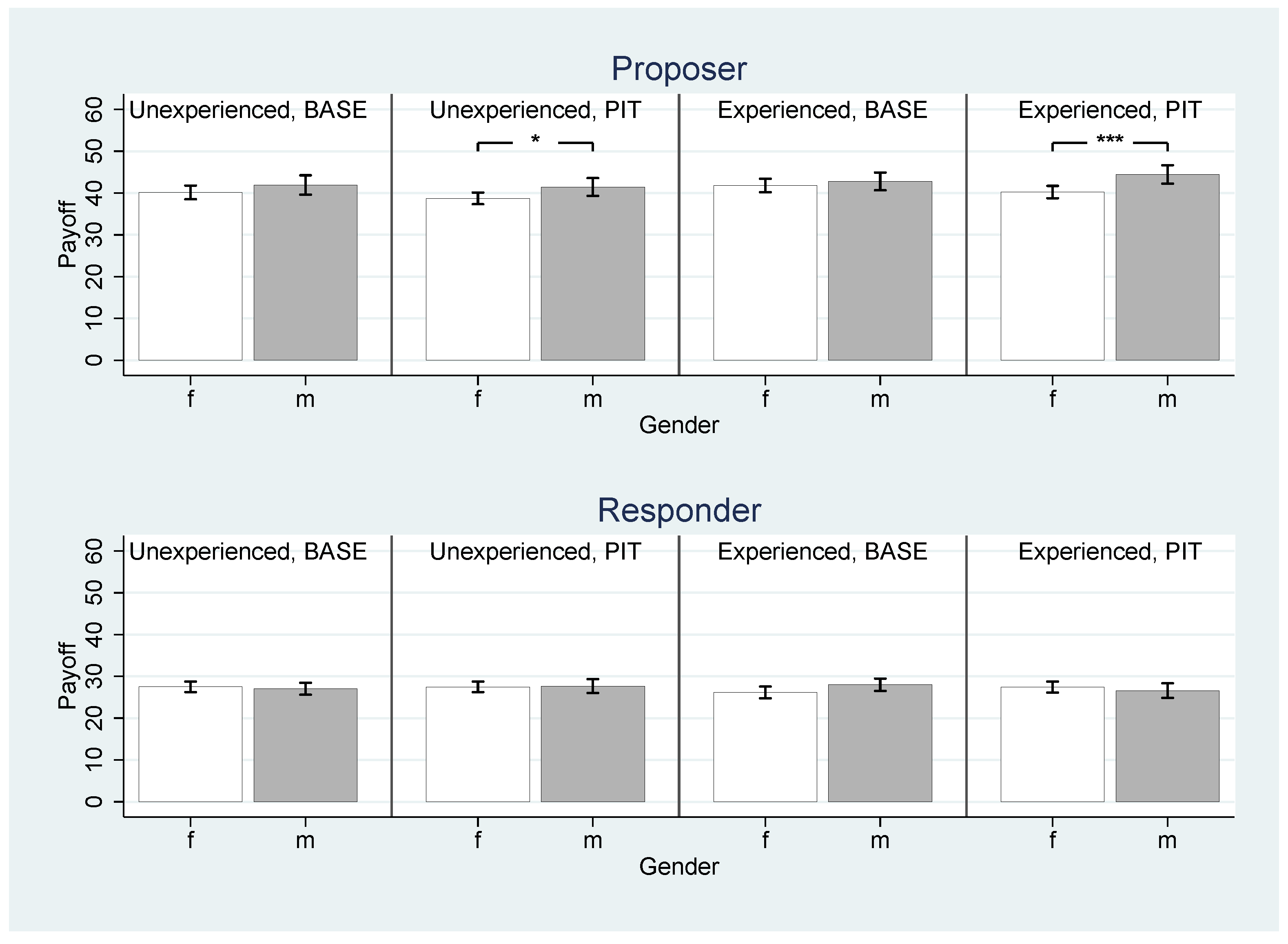
The upper panel of
Figure 1 shows that male proposers, without and with experience, earned slightly more on average than female proposers in both treatments. Inexperienced male proposers earned 41.92 tokens in
Base and 41.45 tokens in
Pit, while inexperienced female proposers earned only 40.14 tokens in
Base and 38.73 tokens in
Pit; experienced male proposers earned 42.79 tokens in
Base and 44.47 tokens in
Pit, while experienced female proposers earned only 41.81 tokens in
Base and 40.24 tokens in
Pit (see
Table A2 in
Appendix A). However, the null hypothesis of equal payoffs is rejected for the
Pit treatment only, using a two-tailed
t-test with unequal variances. In particular,
experienced male proposers earned 4.23 tokens more than experienced female proposers (
). This difference amounts to 10.5% of the experienced female proposers’ average payoffs.
By contrast, we find no noticeable gender effects for payoffs earned in the role of responder. As shown in the lower panels of
Figure 1 and
Table A2, responders earned between 26 and 28 tokens on average irrespective of gender, experience, and treatment. Inexperienced male responders in
Base and experienced male responders in
Pit even earned a bit less than female responders (0.46 and 0.85 tokens, respectively), but none of the payoff differences are statistically significant. There is also no difference on aggregate, i.e., when comparing the earnings of women and men in both roles (see the bottom panel in
Table A2).
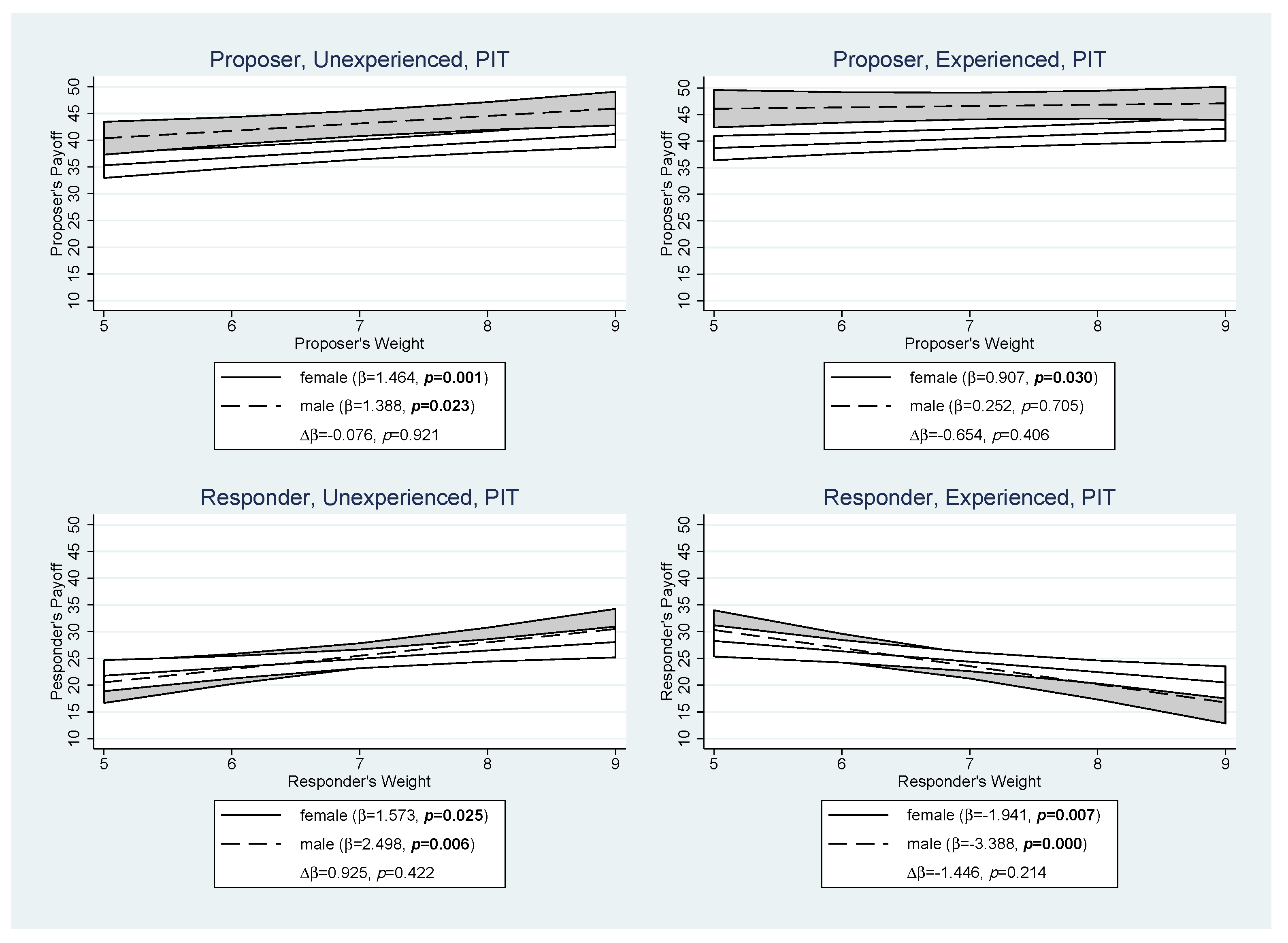
In
Pit, players’ payoffs may additionally be influenced by their nominal voting weights and “power illusion” may reinforce payoff differences (Conjecture 1b).
Figure 2 shows the marginal effect (
) of the voting weight on proposers’ (upper panels) and responders’ (lower panels) payoffs. The marginal effect is estimated by a random effects Tobit regression. There is 1 (of 400) left-censored (i.e., zero payoff) observations for proposers, and there are 374 (of 1600) left-censored observations for responders. Random effects panel regression with session clustered standard errors yields qualitatively identical results.
Figure 2 illustrates again that male proposers tend to earn more than female proposers (Conjecture 1a). For each nominal voting weight, the gender-payoff difference is statistically significant at least at the 10% level (
test at weights 5–9). The regression analysis shows that an extra nominal vote earned inexperienced female and male proposers about 1.40 tokens per nominal vote. For experienced proposers, this relationship is much weaker for both genders, and it is significant only for female proposers (0.91 tokens per extra nominal vote,
). However, with respect to Conjecture 1b, we must note that the gender difference is not significant (inexperienced,
; experienced,
), i.e., the nominal weighting does not increase the difference between female and male proposers.
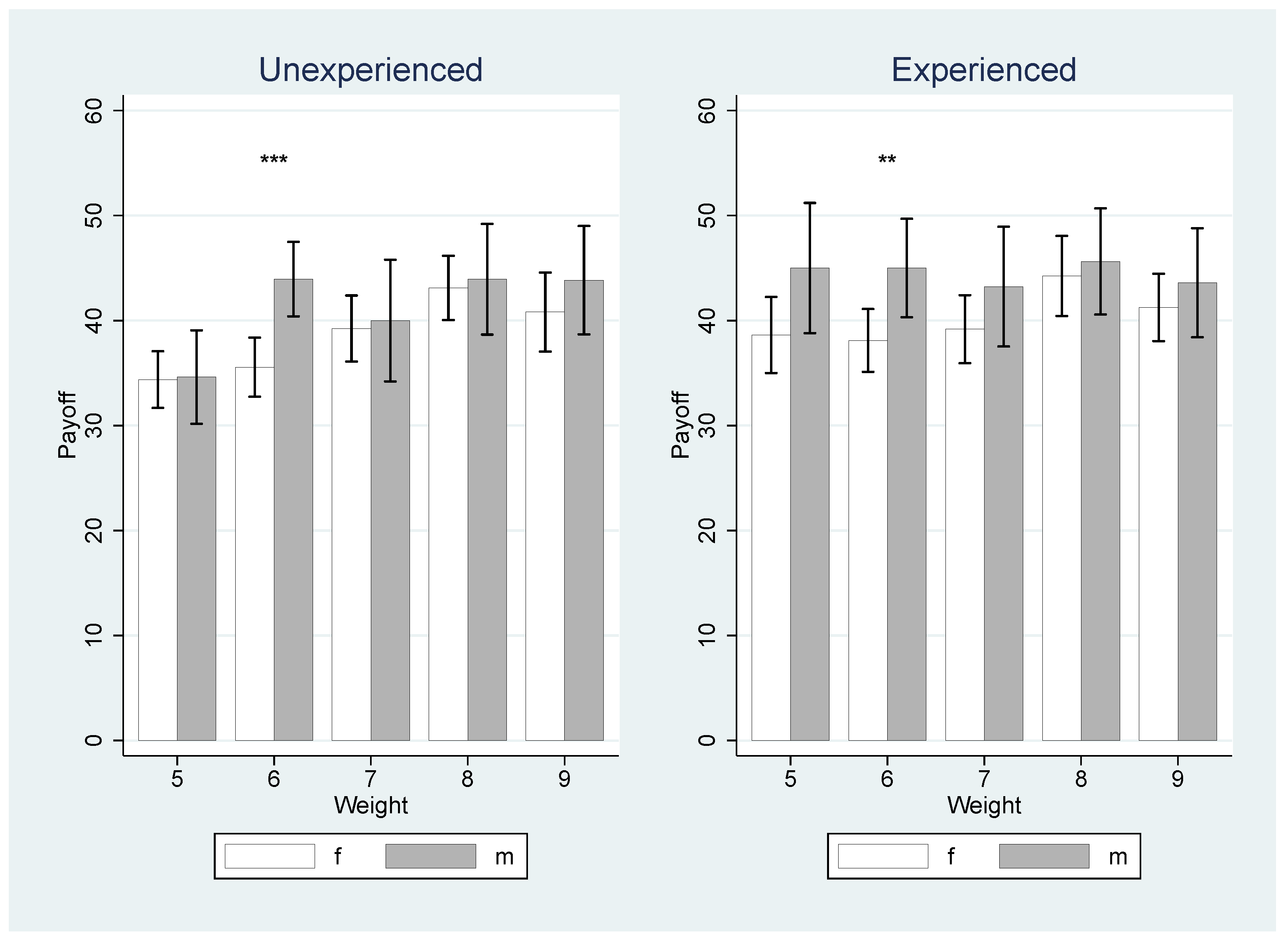
Figure A1 in
Appendix A shows proposer payoffs by gender and weight, with women’s poorer performance in
Pit attributed primarily to their low earnings in the weight-6 role.
The lower panel of
Figure 2 again confirms that women and men earned the same as responders. However, it also shows an interesting pattern in which nominal vote weights had opposite effects on the payoffs of inexperienced and experienced responders. Inexperienced responders earned significantly more when they had higher nominal vote weights (women: 1.57 tokens per nominal vote; men: 2.50 tokens). In contrast, experience made higher nominal vote weights a disadvantage (female: 1.94 tokens; male: 2.54 tokens). Although this effect appears to be more pronounced for male respondents, the gender interaction with vote weight is not significant for both inexperienced and experienced respondents and therefore does not confirm Conjecture 1b. As proposers did not know the gender of the responders in our experiment, the (insignificant) gender difference must be due to responder behavior, which we will discuss in
Section 3.3.
The above pattern regarding the effect of experience is explained by the fact that high-vote-weight responders’ likelihood to receive an offer decreased over time and, analogously, low-vote-weight responders became more likely to receive an offer (see
Table A3 in
Appendix A). The effect is especially strong in nominal-weight-9 responders, whose chance to receive an offer dropped from 85.5% to 66.7% (
). Hence, significantly less experienced than inexperienced nominal-weight-9 responders voted “yes” on the final allocation (49% vs. 67.5%,
), and significantly more experienced nominal-weight-5 and nominal-weight-6 responders voted “yes” (see
Table A4 in
Appendix A).
Result 1: Regarding Hypothesis 1, we conclude that
- (a)
Male proposers on average earn more tokens than female proposers only in the Pit treatment (with nominal voting weights). Experience does not diminish the gender-payoff gap. Higher nominal voting weights have a positive impact on the payoffs of proposers of both genders, but they do not alter the gender-payoff gap.
- (b)
Male and female responders earn equal payoffs, both in Base and in Pit. Having a higher nominal voting weight in Pit turns from an advantage to a disadvantage (in terms of tokens earned) with increasing experience. This effect seems to be stronger in male than in female responders.
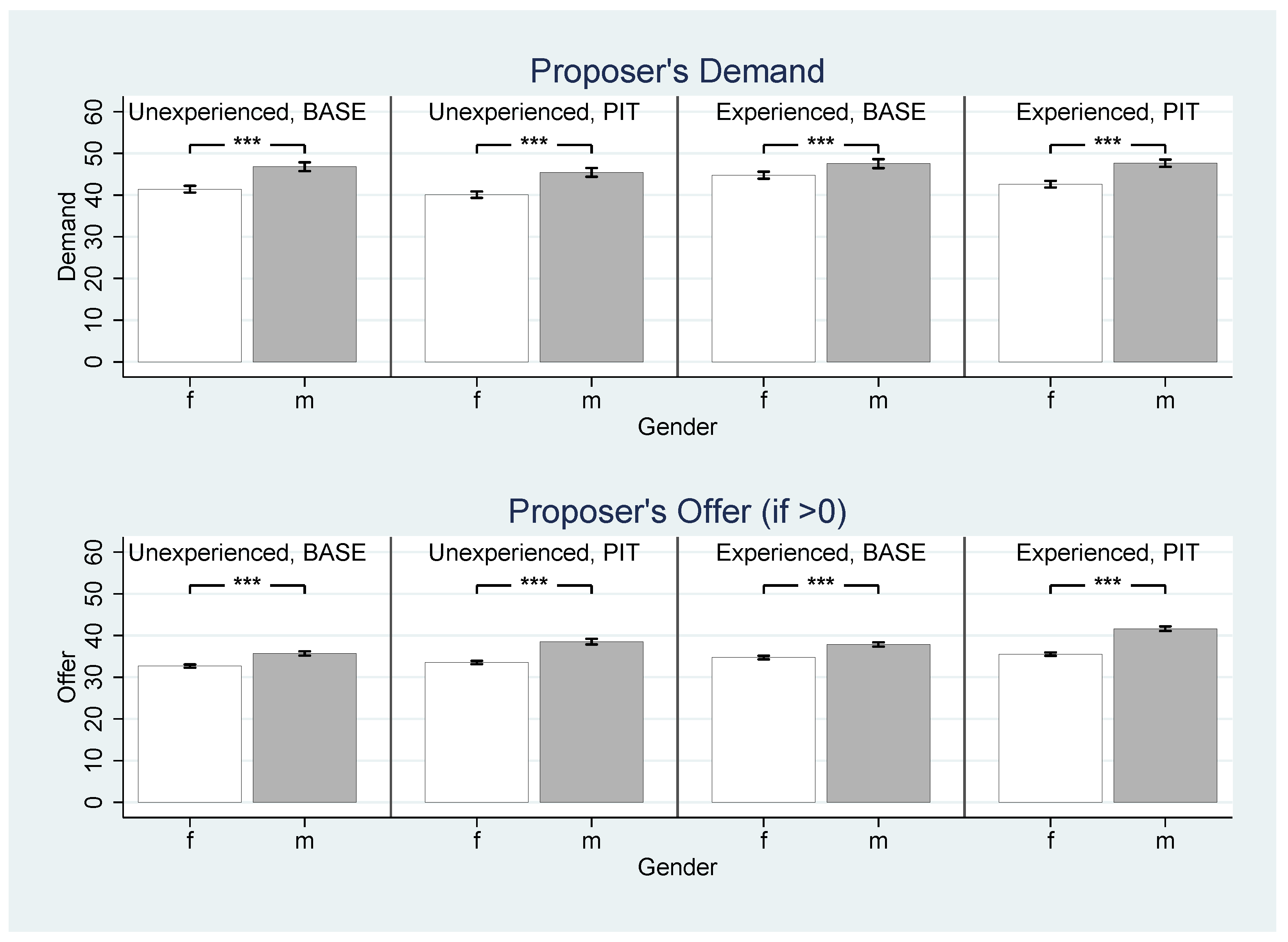
3.2. Proposer Behavior
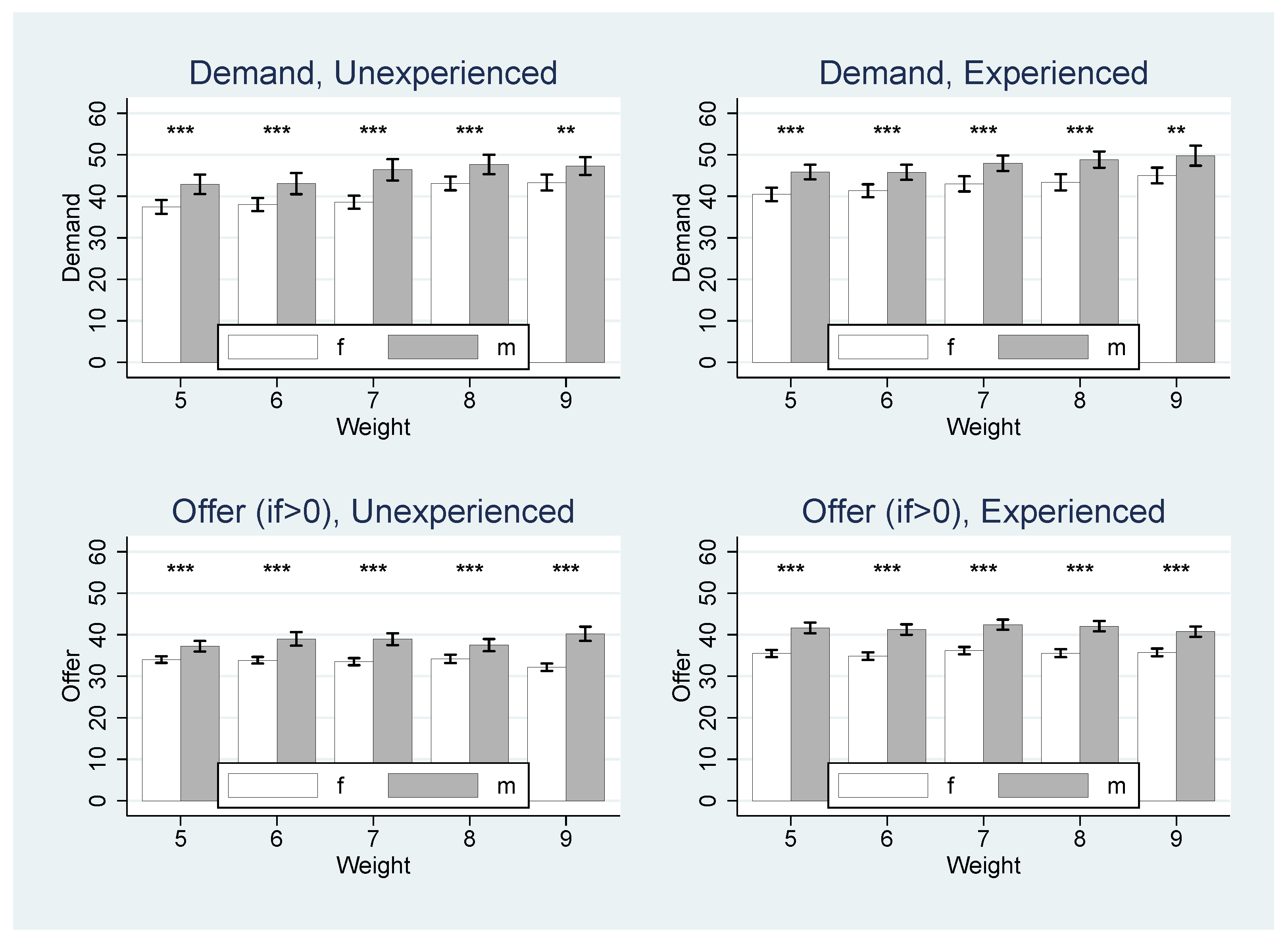
Figure 3 provides proposers’ average demand and average offer to targeted coalition members in the upper and the lower panel, respectively. In line with Conjecture 2a, we find that male proposers generally demanded significantly more for themselves than female proposers. The difference is more than 5 tokens for inexperienced proposers. In
Base, the difference shrinks to 2.76 tokens when proposers become experienced, but is still significant. In
Pit, the gap remains large (exactly 5 tokens).
Additionally, the lower panel of
Figure 3 shows that male proposers generally offered
more than female proposers to responders when that responder was included in the proposed coalition. As the total number of tokens was fixed at 150, this implies that, on average, male proposers chose
smaller coalitions than female proposers. We return to this point when we consider Conjecture 4a in
Section 3.4.
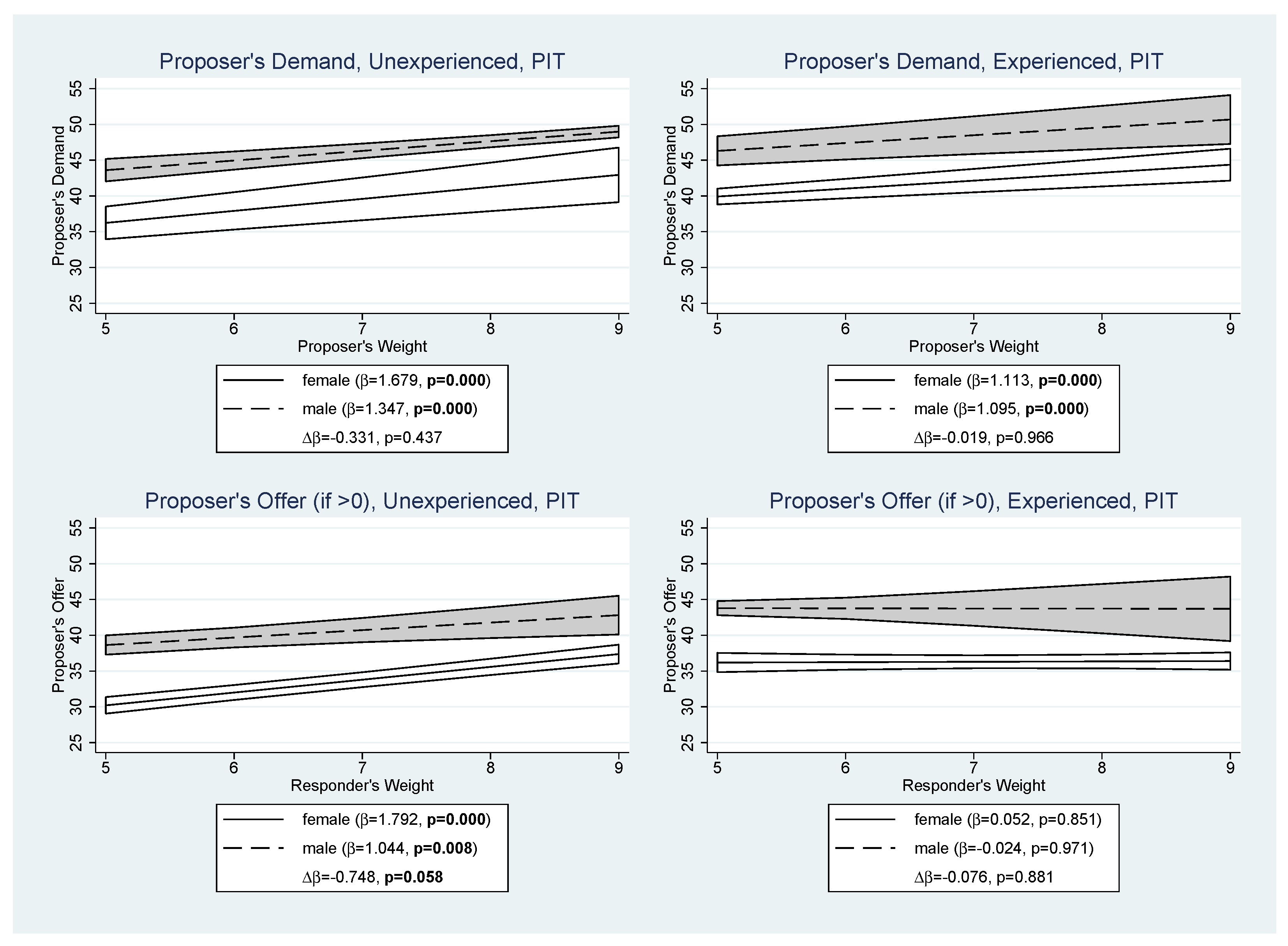
Figure 4 shows how the nominal voting weight influenced proposer behavior in the
Pit treatment. The upper panels show the marginal effect of the proposer’s nominal voting weight on her or his average demand in tokens. The lower panels show the marginal effect of the responder’s nominal weight on the proposer’s average offer in tokens. Both marginal effects are estimated by random effects panel regressions with session clustered standard errors (due to the exclusion of zeros, censoring is irrelevant).
The upper panels not only confirm that male proposers allocated more to themselves than female proposers, but also show that an extra nominal vote increased the proposer’s demand by up to 1.70 tokens. The relationship between nominal voting weight and demand became less steep for experienced proposers (
,
) but is still significant. There were no gender differences concerning the impact of the nominal voting weight on proposer demand (inexperienced:
,
; experienced:
,
). As an alternative perspective on behavior in
Pit, the upper panel of
Figure A2 in
Appendix A shows proposer’s demand by gender and weight.
The lower panels of
Figure 4 show that inexperienced proposers offer more to potential coalition members the larger their nominal voting weight (female: 1.79 tokens per vote; male 1.04 tokens per vote). The gender difference of 0.75 tokens is significant (
), but disappears for experienced players. We show proposer’s offer by gender and responder’s weight in the lower panel of
Figure A2 in
Appendix A.
Result 2: Regarding Hypothesis 2, we conclude that
- (a)
Male proposers on average allocate more tokens to themselves than female proposers. Experience diminishes this gender difference only in the Base treatment. In Pit, both genders increase their demands with increasing nominal voting weights even if they are experienced.
- (b)
Contrary to our Hypothesis 2b, nominal weighting does not affect male and female proposers differently.
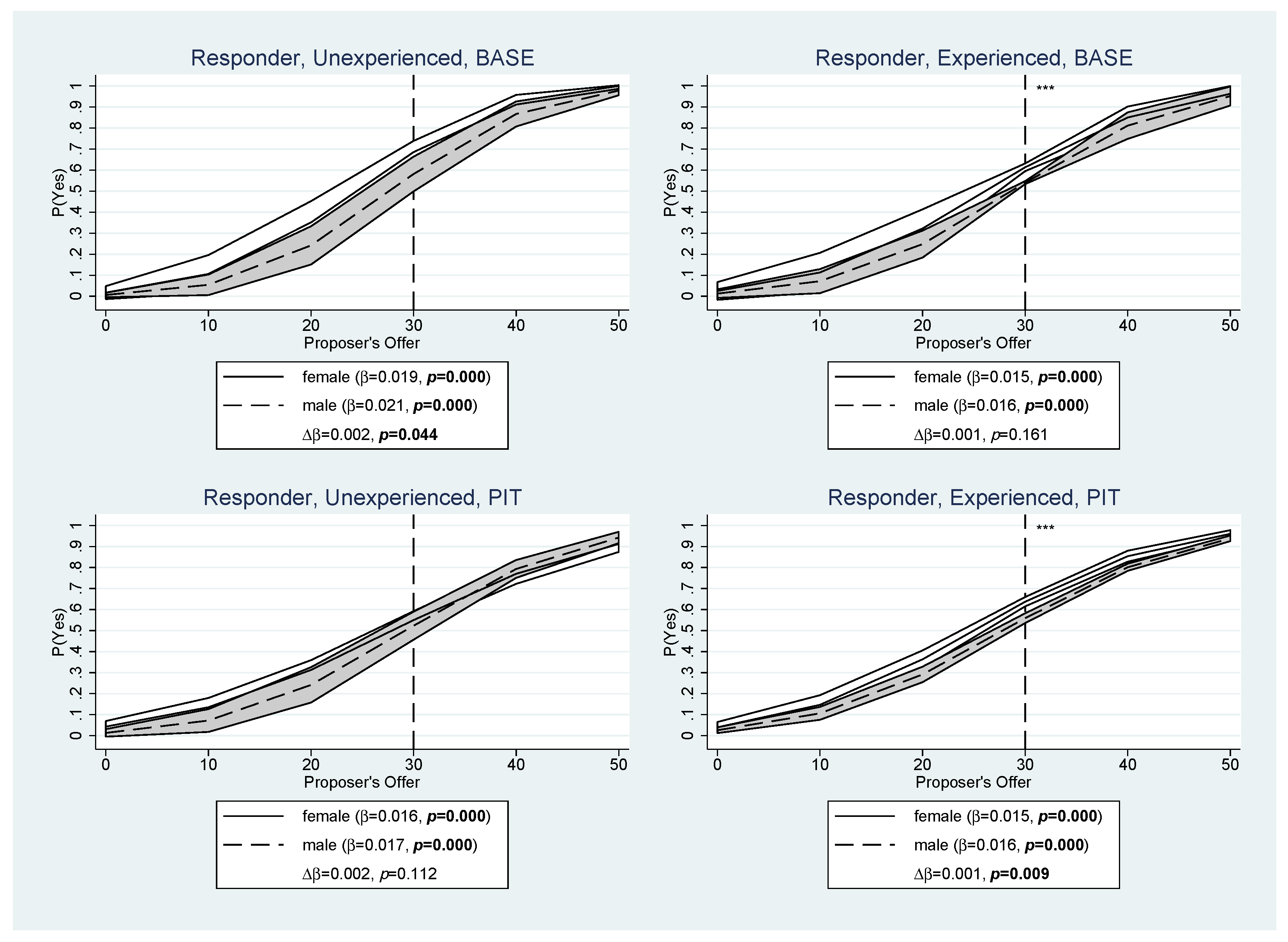
3.3. Responder Voting Behavior
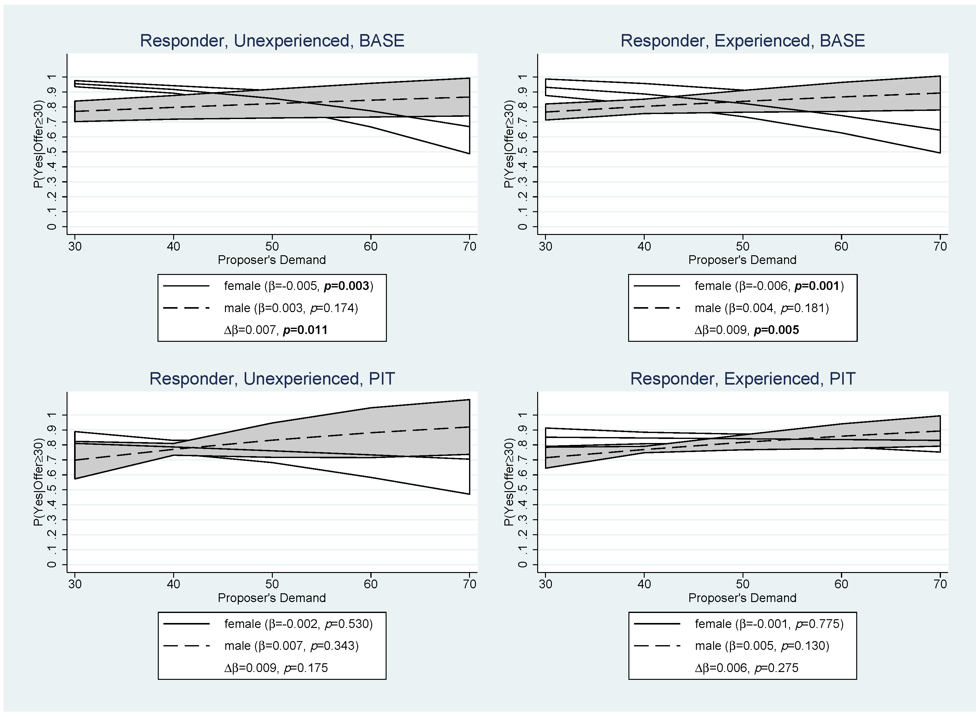
Responders could either vote “yes” in order to accept a proposal or “no“ in order to reject a proposal.
Figure 5 shows how responders reacted to the proposer’s offer in terms of the average probability to vote “yes” on a certain offer in tokens. Note that there were almost no offers exceeding 50 tokens, which is one third of the pie. Interestingly, even offers below 30 tokens had some chance to be accepted. Offers of 50 tokens were almost always accepted.
Although the 90% confidence intervals for female responders and male responders, in white and gray shade, respectively, largely overlap, the graphs indicate that female responders were inclined to accept lower offers than male responders. This finding supports our Conjecture 3a. In fact, the estimated coefficients show that male responders’ reaction function to the proposer’s offer was steeper than that of female responders in all four settings. For example, in inexperienced Base, the average marginal effect of one extra token on was 1.9% for female responders and 2.1% for male responders. Still, the gender difference is significant at the 10% level only in inexperienced Base and experienced Pit.
We also estimated the gender difference for
at an offer of 30 tokens (see the dashed line at
). The respective means, standard errors, and tests are displayed in
Table A6 in
Appendix A. The graphs and the numbers reported there clearly demonstrate that experienced females were significantly more likely to vote “yes” on a 30-token proposal than experienced males (7.3% in
Base, 7.8% in
Pit). In light of this, we consider Conjecture 3, that women accept lower offers than men, as being confirmed by the data, at least for experienced responders.
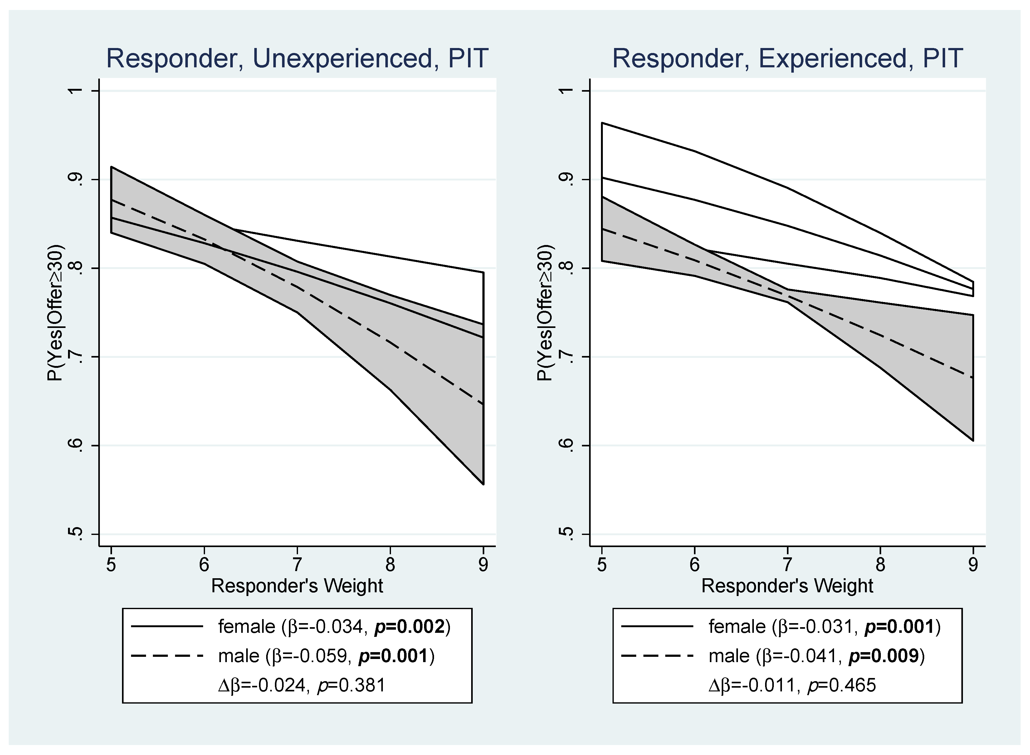
Figure 6 additionally shows how respondents reacted to offers of
at least 30 tokens (the game theoretic prediction for an acceptable offer) in
Pit given their own nominal vote weight. The plots clearly show that respondents with higher nominal vote weights were less likely to accept such an offer, even if they were experienced. For example, inexperienced male respondents decreased their likelihood of voting “yes” by almost 6% per nominal vote (marginal effect). Thus, the analysis confirms Conjecture 3b. There are no significant gender differences, although the effects of nominal vote weight were somewhat weaker for female respondents.
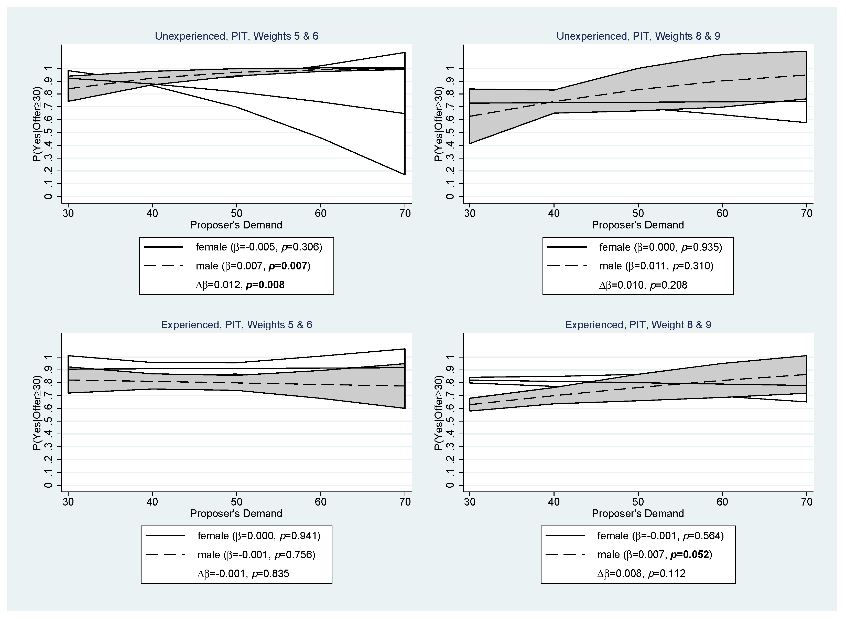
Next, we examine how responders responded to the proposer’s demand (Conjecture 3c).
Figure 7 focuses on responders who received an offer of at least 30 tokens, i.e., who were involved in a coalition and received an offer that should be accepted from a game theoretic perspective. The figure shows that inexperienced and experienced female responders in the
Base treatment reacted negatively to the proposer’s demand. For female responders, the probability of accepting an offer shrank by about −0.5% to −0.6% per token demanded by the proposer. For the
Pit treatment, the response of female responders was also negative, but much weaker and not significant. The response of male responders to the proposer’s demand was not significant in either treatment. Thus, we conclude that only female responders reacted negatively to the proposer’s demand. However, in the
Pit treatment, this effect appears to have been masked by the higher complexity of the decision task with nominal vote weights. Breaking down responder behavior in
Pit by responders’ nominal voting weights does not reveal additional insights and is therefore relegated to
Figure A3 in
Appendix A.
Result 3: Regarding Hypothesis 3, we conclude that
- (a)
Female responders accept lower offers than male responders.
- (b)
Responders’ acceptance thresholds increase with their nominal voting weights.
- (c)
In contrast to male responders, female responders, who receive an offer of at least 30 tokens, are more likely to react negatively to the proposer’s demand.
3.4. Coalition Size
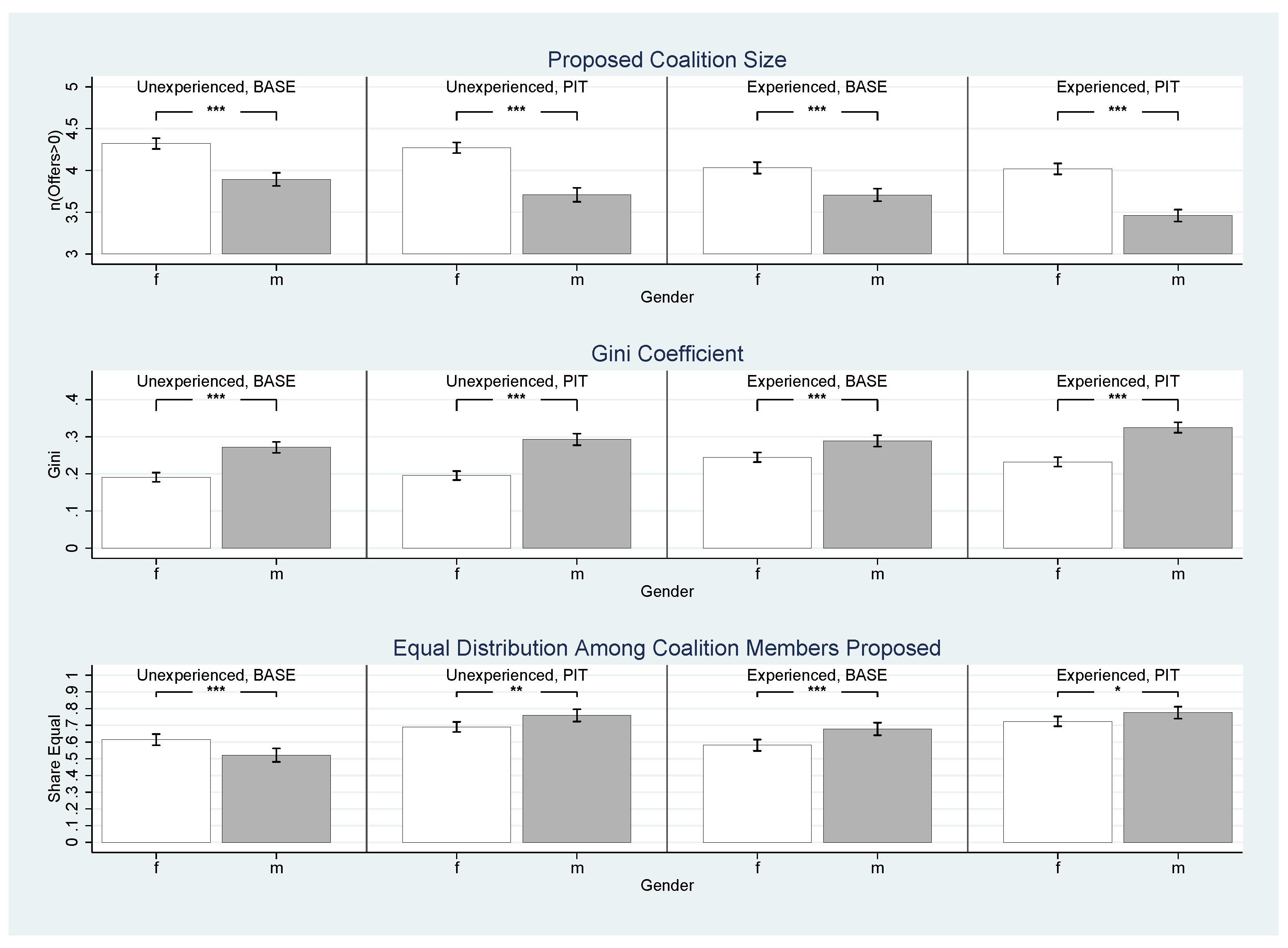
Finally, we turn to the effects of gender on the proposed coalition size.
Figure 8 shows the proposed coalition sizes in the top panels, the average Gini coefficient of the proposed distributions in the middle panels, and the proportion of the same distributions among coalition members in the bottom panels, by experience, treatment, and gender. Coalition size is defined as the number of players, including the proposer, who receive an offer greater than zero. The (discrete) Gini coefficient is a measure of inequality normalized to the interval
, with higher values indicating greater inequality. It is calculated using the formula
, where
is the number of players,
is the average payoff,
,
is the proposed payoff of player
i, and the payoffs are increasingly ordered. The fraction of the proposed equal distribution refers only to the coalition members. That is, the proposal
corresponds, up to permutations, to a uniform distribution in a size 3 coalition, the proposal
is a uniform distribution in a size 4 coalition, and
in the large coalition of all five players.
Figure 8 clearly confirms Conjecture 4a that female proposers proposed larger coalitions than male proposers. The gender difference is highly significant for both treatments and for inexperienced and experienced proposers. The middle panels of the figure show that female proposers on average proposed significantly less unequal allocations. For example, in experienced PIT, we have
and
, leading to a highly significant difference of
(
). The lower panels of the figure, however, indicate that, except for those in the inexperienced
Base classification, female proposers proposed an equal distribution
within the coalition significantly less often compared to male proposers. In other words, female proposers sought to build broader, more equal coalitions by offering to more respondents, but at the same time they sought to claim a
relatively larger share for themselves.
Result 4: Regarding Hypothesis 4, we conclude that
- (a)
Female proposers form more inclusive coalitions.
- (b)
Coalitions formed by female proposers are less unequal across all players, but more unequal within the coalition.
3.5. Discussion
One may wonder whether the female strategy—proposing more inclusive coalitions which involve more within-coalition payoff inequality—was more successful than the male strategy—proposing minimum winning coalitions with low within-coalition payoff inequality. If so, adopting this proposer behavior could be motivated by risk aversion [
28]. To shed light on this, we compare the acceptance rates of minimum winning coalitions (
) and grand coalitions (
). Together, these two types of coalitions accounted for more than 95% of all proposed coalitions. In
Base with inexperienced players, we find that minimum winning coalitions were accepted at a higher rate and grand coalitions at a lower rate than would be expected under the assumption of independence (
,
). The negative association between acceptance rate and size of the proposed coalition disappeared with increasing experience (
,
). In
Pit, however, experience tended to reinforce the relatively higher acceptance rate of minimal gain coalitions compared to large coalitions (inexperienced:
,
; experienced:
,
). Thus, if anything, proposing larger coalitions had a
negative effect on acceptance rates.
Did proposing an equal distribution of payoffs among coalition members change the probability that the proposal was adopted? For Base, the answer is “no” (inexperienced: , ; experienced: , ). In contrast, the response in Pit is “yes” (inexperienced: , ; experienced: , ). Thus, in Pit, male proposers clearly had a greater chance of having their proposals passed because they more often proposed small coalitions with equal payoff distributions among coalition members, i.e., .
As experienced female proposers continued to propose more inclusive coalitions even though these had lower acceptance rates, exclusion aversion seems a more plausible explanation of their behavior than risk aversion (i.e., minimizing the chance that their own proposal is rejected). Note, however, that the evidence is only suggestive, as we do not know players’ beliefs regarding the probability of rejection.
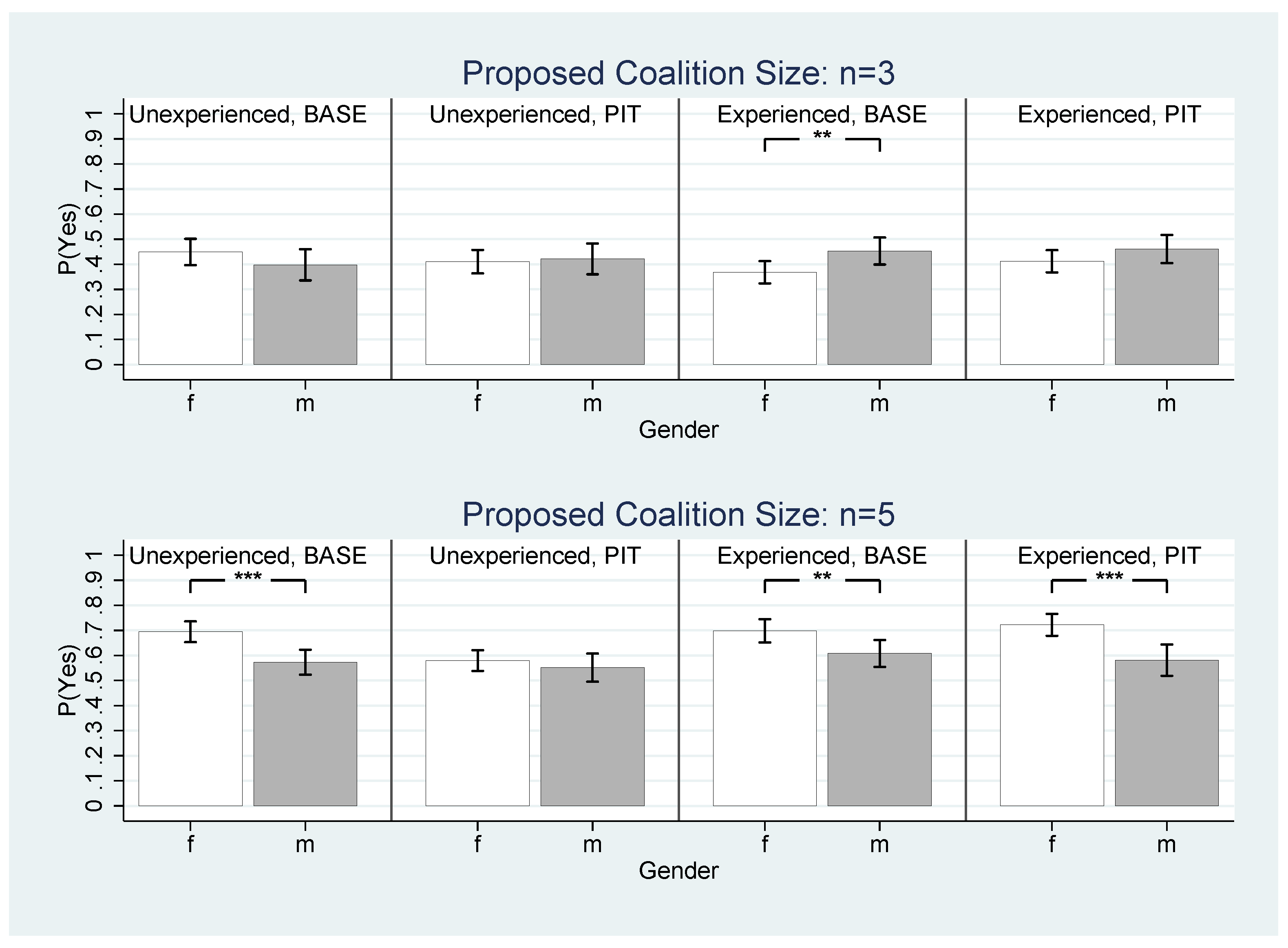
Figure 9 and
Table A8 in
Appendix A further address this question by comparing the individual probabilities to accept a proposal between female and male responders for given coalition size
n. The upper panels show the individual acceptance rates of minimum winning coalitions (
). Analogously, the lower panels show graphs and numbers for the grand coalition (
). With respect to minimum winning coalitions, there is almost no gender difference. If at all, male responders were a bit more inclined to accept minimum winning coalitions. In experienced
Base, the difference of 8.5 percentage point is significant (
). In contrast to this, female responders were, except for inexperienced
Base, significantly more likely to accept grand coalitions; in experienced
Pit the gender difference rises to 14.1 percentage points (
). From this, we can conclude that female players showed a strong preference for including all group members in the coalition, both in their roles as proposers and responders. This suggests that women prefer less inequality in the overall group compared to men.


