Identification and Control of Game-Based Epidemic Models

Abstract

The effectiveness of control measures against the diffusion of the COVID-19 pandemic is grounded on the assumption that people are prepared and disposed to cooperate. From a strategic decision point of view, cooperation is the unreachable strategy of the Prisoner’s Dilemma game, where the temptation to exploit the others and the fear of being betrayed by them drives the people’s behavior, which eventually results in a fully defective outcome. In this work, we integrate a standard epidemic model with the replicator equation of evolutionary games in order to study the interplay between the infection spreading and the propensity of people to be cooperative under the pressure of the epidemic. The developed model shows high performance in fitting real measurements of infected, recovered and dead people during the whole period of COVID-19 epidemic spread, from March 2020 to September 2021 in Italy. The estimated parameters related to cooperation result to be significantly correlated with vaccination and screening data, thus validating the model. The stability analysis of the multiple steady states present in the proposed model highlights the possibility to tune fundamental control parameters to dramatically reduce the number of potential dead people with respect to the non-controlled case.

1. Introduction

The recent coronavirus pandemic enforced the application of control measures for restraining the virus diffusion. The most successful measures for weakening and reducing the infection aim at preventing people from getting infected or at least to get the disease in a weak form, and consist, on the one hand, of the adoption of medical treatment protocols and of vaccination, and, on the other hand, of avoiding behaviors which favour virus spreading, such as social distancing, movement reduction, mask wearing, and so on [1]. The application of any control measures requires the organization of suitable information campaigns aimed at inducing people to adopt correct behaviors against the pandemic. To make these campaigns effective, people must behave cooperatively with respect to the limitations and requirements imposed by the deputed institutions and governments. Unfortunately, more often, when taking decisions under strong pressure, such as, for example, in the initial phases of the pandemic, the requirement of strong efforts may activate in the population selfish and conservative mechanisms, which often lead to the temptation to exploit the cooperative behavior of the others and to the fear of being betrayed by their incorrect conduct. An example of these mechanisms is represented by the panic buying that arose at the beginning of the COVID-19 pandemic (see, for example, [2]). Similarly, correct campaigns should be able to convince citizens that the costs of vaccination are less than the rewards, resulting in the possibility to recover almost normal life styles and well-being. Avoiding selfish mechanisms and promoting good ones requires fostering altruistic and cooperative feelings.

Emerging of cooperation is recognized as challenging in many different fields [3,4], and Evolutionary Game Theory (EGT) represents a natural mathematical framework to model this problem. Indeed, it provides a rigorous methodology for studying strategic interactions among people evolving over time [5,6]. The evident drawbacks of selfish behavior are highlighted in the defective Prisoner’s Dilemma game, in both the mean field formulation [7,8], and for interconnected populations [9,10]. The influence of social networks on the dynamics of cooperation in evolutionary games has been deeply investigated [11,12,13,14,15].

With specific reference to the people’s behavior in the management of an epidemic, an extensive review of the literature on behavioral epidemiology is presented in [16], where the possibility to include its effect in mathematical models is discussed from a methodological point of view, pointing out that concrete models should account for many factors, thus significantly increasing the number of parameters and equations. Models grounded on game theory have been proposed for analysing and predicting vaccination behavior [17,18]. In [19], a suitable game is introduced to account for the reward of social distancing in vulnerable and non-vulnerable agents, while [20] studies the optimal strategies of people to contain the epidemic spreading by appropriately planning their movements to avoid strongly infected places.

Moreover, the emergence of the COVID-19 epidemic fostered the development of mathematical models for the integration of the standard [21] or adapted [22,23] SIR and SIRS models with suitable control measures for contrasting the infection in different ways. For example, in [24] the role of a network on disease spreading is analyzed, in [25] optimal control measures are identified by assuming networked populations, while in [26] an analysis of strategic behavior during the COVID-19 pandemic was developed from an economic perspective. Additionally, in [27] the strong influence of collective behavioral patterns of the population in epidemic spreading was highlighted by stochastic models.

In this paper, we propose the integration of a SIRS epidemic model with a replicator equation, describing the evolution over time of cooperation in large populations. Despite the above large literature taking reasonably into account the presence of a network and its role in the disease spreading, in this paper we focus on the interplay between epidemiological and social dynamics from a mean field point of view, since our main objective is to find simple mechanisms regulating people’s behavior and cooperation during a pandemic event in a large and complex nation like Italy. Similar approaches have been taken into account in [28], and deeply studied in [29], where the relationship between control measures, vaccine hesitation, information retrieval, and policy making has been investigated to enforce cooperative behavior aimed to reduce the virus’ spread.

A convincing motivation for developing models like the one proposed in this paper is provided in [30], where the authors highlighted that the effects of shield immunity and economic shutdowns are complementary, such that governments should pursue them in tandem. In a more theoretical setting [31], the SIR model has been coupled with the replicator equation of evolutionary games. Similarly to our study, people’s behavior is influenced by the infection strength, and, in particular, by evaluating the infection rates of cooperators and defectors, including the corresponding risks and costs. Since evaluating the infection rates is a difficult task for people, the model proposed in this paper assumes that cooperative/defective decisions are driven by easily retrievable information, such as the number of dead or infected individuals. A similar reasoning for spontaneous adoption of quarantine states has been done in [32].

Developing this new model may help to formalize and understand better the twofold feedback mechanisms between epidemic spreading and people’s behavior from a theoretical point of view. On one hand, the infection rate is assumed to depend on the propensity to cooperate by respecting the control and recovery measures taken by the governments. In our case, it decreases when cooperation increases. On the other hand, the parameters of the game payoff matrix depend on the strength of the epidemic at any time; thus, the higher is the gravity of the epidemic, the higher is the propensity to cooperate, despite the limitations and costs imposed by the government’s directives. Overall, the switches from the Prisoner’s Dilemma game to the fully cooperative Harmony game and vice versa are observed.

The remaining of this paper is organized as follows. In the Material and Methods section, the assumptions on which the mathematical model is grounded, together with its theoretical properties, are reported, while the Results section presents the main findings of the research. Finally, some concluding remarks are provided in the Conclusions section.

2. Materials and Methods

A population of M individuals, split into 6 classes, is considered:

• S: Susceptible individuals;
• U: Undetected infected individuals;
• I: Detected infected individuals (hospitalized or quarantined);
• R: Recovered individuals;
• D: Dead individuals,

where $S+U+I+R+D=M$. According to the literature on epidemic models [21], and to significant recent results [25,33], we start from the following epidemic model of COVID-19:

$$\left\{\begin{array}{cc}\dot{S}\hfill & {\displaystyle =-\beta \frac{SU}{M}+\alpha R}\hfill \\ \dot{U}\hfill & {\displaystyle =\beta \frac{SU}{M}-\gamma U-\tau U}\hfill \\ \dot{I}\hfill & =\tau U-\zeta I-\omega I\hfill \\ \dot{R}\hfill & =\gamma U+\omega I-\alpha R\hfill \\ \dot{D}\hfill & =\zeta I\hfill \end{array}\right.,$$

(1)

where $\beta$ is the infection rate, $\alpha$ is the drop immunity rate, $\gamma$ is the spontaneous healing rate, $\tau$ is the detection rate, $\omega$ is the healing rate of detected infected persons, and $\zeta$ is the death rate. According to [25], we assume that, for the COVID-19 case, some model parameters and the reproduction number

$$\mathcal{R}\left(t\right)=\frac{\beta }{\gamma +\tau },$$

(2)

are time varying. For the sake of simplicity, in the rest of the paper, we will refer to (1) as Infection Model (IM).

2.1. How Epidemics Influence People’s Behavior

In an epidemic context, it is reasonable that individuals behave by choosing one of the following two strategies: cooperating (C) or not (N). In our study, the first option consists of respecting the restrictions imposed by the deputed institutions for constraining the spread of the disease, while the second indicates people adopting habits not fully aligned with the sanitary guidelines. We denote by $x\in [0,1]$ the share of cooperators, and by $z=1-x$ the share of non cooperators.

In Game Theory, the decision mechanism is ruled by a payoff matrix, describing the outcome of the interaction between couples of players randomly chosen in the population [34]. In the investigated context, the payoff matrix has been chosen following [24]:

$$B=\left[\begin{array}{cc}1& \mathcal{S}\\ \mathcal{T}& 0\end{array}\right],$$

(3)

where, the first row contains the payoffs for cooperation (C) and the second one the reward for defection/non-cooperation (N) for player 1. Similarly, the columns of the payoff matrix are related to the choices of player 2. More specifically, $\mathcal{T}$ corresponds to the temptation to defect and $\mathcal{S}$ is the “sucker’s payoff”, embodying the fear of being betrayed by others. Player 1 earns 1 if both cooperate, $\mathcal{T}$ if he defects and the opponent cooperates, $\mathcal{S}$ if he cooperates and the opponent defects, or 0 if both players defect.

It is useful to introduce the net payoffs for cooperation, ${\sigma }_C=1-\mathcal{T}$, and for defection, ${\sigma }_N=-\mathcal{S}$. Then, for ${\sigma }_C<0$ (i.e., the temptation to defect is higher than the reward for mutual cooperation) and ${\sigma }_N>0$ (i.e., the fear of being betrayed is significantly high), the payoff matrix (3) embodies a Prisoner’s Dilemma game, where defection is dominant, while for ${\sigma }_C>0$ and ${\sigma }_N<0$, the game switches to a Harmony game, and cooperation is the dominant strategy [34].

In the epidemic context, the Prisoner’s dilemma game can be restated as follows: if two individuals meet, and adopt good practices (i.e., social distancing, mask wearing, getting vaccinated), then they both get a normalized reward equal to 1, corresponding to the preservation of their own health. In contrast, if two individuals meet, and, for instance, neither of them wear a mask, then there is a high probability that, if one is infected, the second will get infected too. In this case, both players earn a payoff equal to 0, i.e., their health has not been preserved. Now, suppose that one of them knows that the other is respecting the containment measure; then (s)he will be tempted not to respect the good practices. In this case, the “free rider” will earn $\mathcal{T}>1$, which corresponds to her/his own safety (the other will not infect her/him, and hence her/his payoff is equal to 1) plus, for instance, the feeling of freedom of staying without mask (payoff equal to $\mathcal{T}-1=-{\sigma }_C>0$). On the other hand, the “good citizen” is not protected—the other can be infected and can infect her/him too. Thus, s(he) will earn 0 minus the feeling of being the only one respecting the sanitary guidelines (payoff equal to $\mathcal{S}=-{\sigma }_N<0$). When we move to the Harmony scheme, the outcomes for the hybrid case (a cooperator meets a defector) change, since $\mathcal{T}<1$ and $\mathcal{S}>0$.

Given a generic game, the dynamical evolution of the strategies within a well mixed population can be described by the Replicator Equation (RE) [5,6,34], which reads as follows:

$$\left\{\begin{array}{cc}\dot{x}\hfill & =x({\pi }_C-\overline{\pi })\hfill \\ \dot{y}\hfill & =y({\pi }_N-\overline{\pi })\hfill \end{array}\right.,$$

(4)

where

$$\left[\begin{array}{c}{\pi }_C\\ {\pi }_N\end{array}\right]=B·\left[\begin{array}{c}x\\ z\end{array}\right]=\left[\begin{array}{c}x+\mathcal{S}z\\ \mathcal{T}x\end{array}\right]=\left[\begin{array}{c}x-{\sigma }_{N}z\\ (1-{\sigma }_C)x\end{array}\right]$$

represent the average payoffs ${\pi }_C$ and ${\pi }_N$ collected by the share of cooperative and non-cooperative individuals, respectively, while

$$\overline{\pi }=x{\pi }_C+z{\pi }_N=x^2+(\mathcal{T}+\mathcal{S})xz=x^2+(1-{\sigma }_C-{\sigma }_N)xz,$$

is the average payoff of the whole population. When ${\pi }_C$ is bigger than $\overline{\pi }$, the time derivative of x is positive, and hence x increases over time. At the same time, by the definition of $\overline{\pi }$ it follows that if ${\pi }_C>\overline{\pi }$, then ${\pi }_N<\overline{\pi }$, and hence y decreases over time. Symmetric arguments hold for the opposite situation (${\pi }_C<\overline{\pi }$). Coherently with the payoff matrix (3) and Equation (4), cooperation evolves towards full defection ($x=0$ and $z=1$) for the Prisoner’s Dilemma case or towards full cooperation ($x=1$ and $z=0$) for the Harmony game.

It is natural to assume that the ruling parameters $\mathcal{T}$ and $\mathcal{S}$ vary with respect to people’s perception on the infection strength, reasonably measured by the state variables I and D of the IM model (U is not observable, since it corresponds to the number of undetected infected people). In this regard, we can assume that the payoff matrix (3) depends on I and D, i.e., $B=B(I,D)$, and that it changes from a Prisoner’s Dilemma game to a Harmony one when the value of $I+D$ exceeds a given activation threshold a:

$${\sigma }_C(I,D)={\sigma }_C^{0}G(I,D)$$

(5)

and

$${\sigma }_N(I,D)={\sigma }_N^{0}G(I,D),$$

(6)

where

$$G(I,D)=\frac{I+D-a}{M}$$

(7)

works as a “game-switching” term, ${\sigma }_C^0>0$, ${\sigma }_N^0<0$ and $0<a<M$.

The term $G(I,D)$ embodies the concept of coevolutionary rules in the evolutionary games framework, thus accounting at the same time for the evolution of strategies, and other related variables, such as the pandemic status [13]. Additionally, the role of $G(I,D)$ in the proposed model recalls the findings reported in [15,35] on the ability of finite and networked populations to self-regulate the behavior when a higher common good (in this case, the public health) should be preserved, thanks to the awareness of individuals.

For $I+D<a$, $B(I,D)$ represents a Prisoner’s Dilemma game, since ${\sigma }_C(I,D)<0$ and ${\sigma }_N(I,D)>0$. That is, when the epidemic is enough low, defection is the “natural” choice, since a perceived weakness of the disease does not justify the adoption of any containment measure. This is coherent with the fact that some governments have been laxer than others in imposing restrictions. In this sense, the threshold a corresponds to an important tuning parameter for the policy-makers, as it can be reduced by means of effective informative campaigns on the real risks of the current sanitary crisis, thus making $I+D>a$. In this case, $B(I,D)$ turns to a Harmony game since ${\sigma }_C(I,D)>0$ and ${\sigma }_N(I,D)<0$.

For the sake of simplicity, we observe that, by exploiting $z=1-x$, and using Equations (5) and (6), we get:

$$\begin{array}{ccc}\hfill {\pi }_C-\overline{\pi }& =& x-{\sigma }_N(I,D)z-(x^2+(1-{\sigma }_C(I,D)-{\sigma }_N(I,D))xz)\hfill \\ & =& x-(1-x){\sigma }_N(I,D)-x^2-(1-{\sigma }_C(I,D)-{\sigma }_N(I,D))x(1-x)\hfill \\ & =& x-(1-x){\sigma }_N(I,D)-x^2-x(1-x)+({\sigma }_C(I,D)+{\sigma }_N(I,D))x(1-x)\hfill \\ & =& -(1-x){\sigma }_N(I,D)+({\sigma }_C(I,D)+{\sigma }_N(I,D))x(1-x)\hfill \\ & =& (1-x)(({\sigma }_C(I,D)+{\sigma }_N(I,D))x-{\sigma }_N(I,D))\hfill \\ & =& (1-x)(({\sigma }_C^0+{\sigma }_N^0)x-{\sigma }_N^0)G(I,D).\hfill \end{array}$$

Then, the RE (4) is reduced to a monodimensional ODE [34] which reads as:

$$\dot{x}=x(1-x)(({\sigma }_C^0+{\sigma }_N^0)x-{\sigma }_N^0)G(I,D).$$

(8)

2.2. How People Behavior Influences the Epidemic

As mentioned before, cooperation corresponds to the adoption of good practices, aimed at reducing the disease spreading, such as, limitation of social interactions, wearing masks, getting vaccinated, and so on. As a consequence, the infection rate $\beta$ of IM varies according to people’s behavior. More specifically, cooperation produces a reduction of the infection rate, while defection leads to its increment. In this work, we assume that the infection rate $\beta$ linearly depends on the cooperation x as follows:

$$\beta \left(x\right)={\beta }_0(1-ex),$$

(9)

where ${\beta }_0$ is the natural infection rate of the disease, while $e\in [0,1]$ weights the influence efficacy of the cooperation on the infection rate. Notice that $\beta \left(x\right)\ge 0\forall x\in [0,1].$ In this case, reproduction number is defined as follows:

$$\mathcal{R}\left(x\right)=\frac{\beta \left(x\right)}{\gamma +\tau }=\frac{{\beta }_0(1-ex)}{\gamma +\tau }={\mathcal{R}}_0(1-ex),$$

(10)

where

$${\mathcal{R}}_0=\frac{{\beta }_0}{\gamma +\tau }$$

(11)

represents the basic reproduction number of the disease. Since x is a function of time, then $\mathcal{R}\left(x\right)$ is time varying, and it reaches the maximum ${\mathcal{R}}_0$ for no cooperation ($x=0$). Moreover, its minimum is equal to

$$\underline{\mathcal{R}}={\mathcal{R}}_0(1-e),$$

(12)

and it is attained in presence of maximum cooperation ($x=1$), i.e., when countermeasures against the disease are effective at the highest level.

2.3. The Infection Game Model

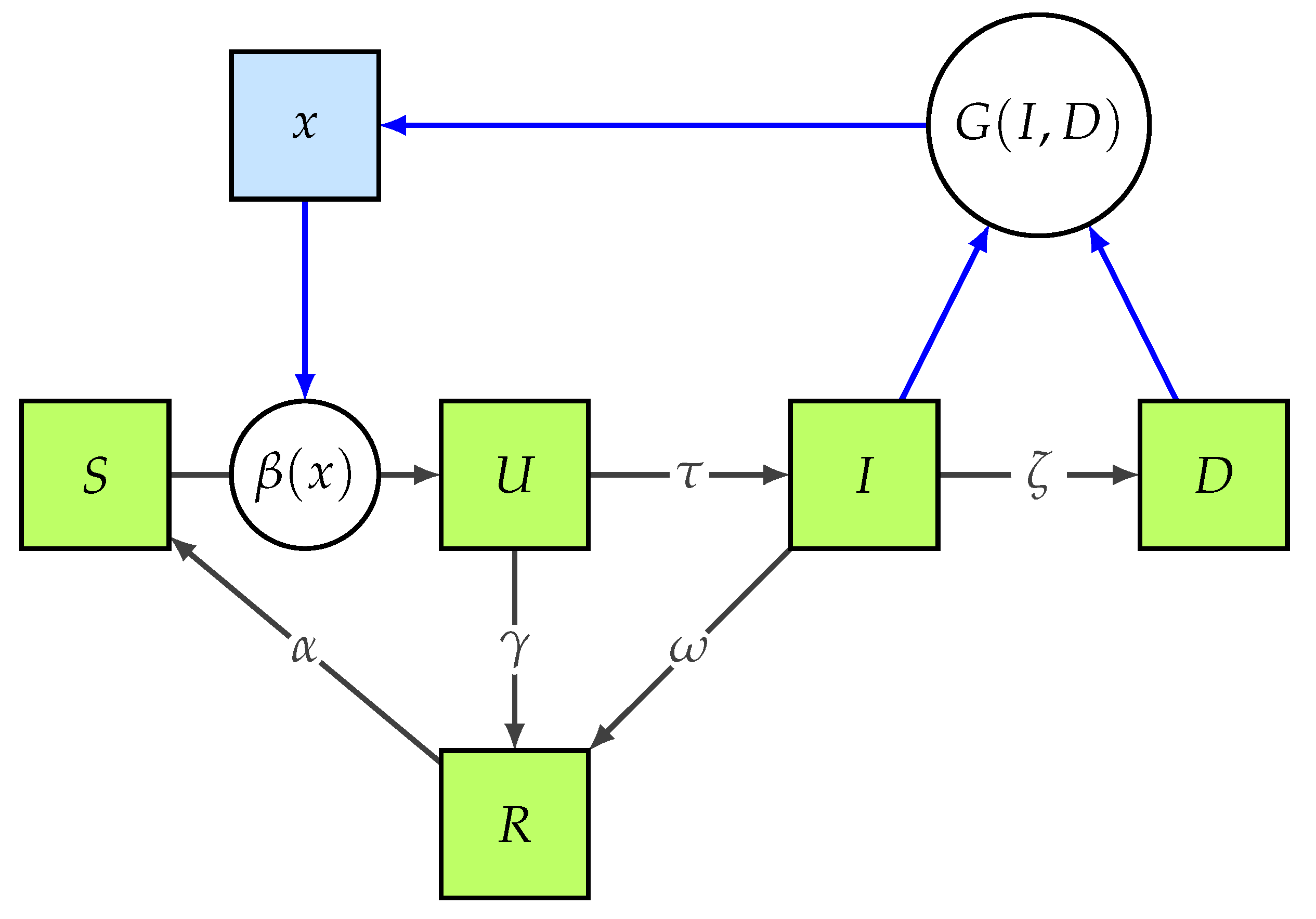
By coupling the standard IM (1) with the RE (8), we get the Infection Game Model (see Figure 1), hereafter called IGM. The model is characterized by the extended state vector $y={[S,U,I,R,D,x]}^{\top }$, and it reads as:

$$\left\{\begin{array}{cc}\dot{S}\hfill & {\displaystyle =-\beta \left(x\right)\frac{SU}{M}+\alpha R}\hfill \\ \dot{U}\hfill & {\displaystyle =\beta \left(x\right)\frac{SU}{M}-\gamma U-\tau U}\hfill \\ \dot{I}\hfill & =\tau U-\omega I-\zeta I\hfill \\ \dot{R}\hfill & =\gamma U+\omega I-\alpha R\hfill \\ \dot{D}\hfill & =\zeta I\hfill \\ \dot{x}\hfill & =x(1-x)(({\sigma }_C^0+{\sigma }_N^0)x-{\sigma }_N^0)G(I,D)\hfill \end{array}\right.,$$

(13)

where $\beta \left(x\right)$ and $G(I,D)$ are defined in Equations (9) and (7), respectively.

It can be easily proven that all the trajectories of system (13) are confined in the feasible set

$$\mathcal{F}=\{y\in {\mathbb{R}}^6:S\ge 0,U\ge 0,I\ge 0,R\ge 0,D\ge 0,S+U+I+R+D\le M,x\in [0,1]\}$$

for all times $t>0$, provided that the initial condition $y\left(0\right)$ belongs to the same set (see [33] for S, U, I, R and D, and [34] for x). Model (13) presents infinite equilibria in $\mathcal{F}$, specifically:

$$\begin{array}{ccc}\hfill y_1^{*}\left(k_1\right)& =& {[M-k_1,0,0,0,k_1,0]}^{\top }\forall k_1\in [0,M]\hfill \\ \hfill y_2^{*}\left(k_2\right)& =& {[M-k_2,0,0,0,k_2,1]}^{\top }\forall k_2\in [0,M]\hfill \\ \hfill y_3^{*}\left(h\right)& =& {[M-a,0,0,0,a,h]}^{\top }\forall h\in [0,1].\hfill \end{array}$$

It is worthwhile noticing that the introduction of a new equation into the epidemic model does not alter the biological mechanisms on which it is grounded. Indeed, at steady state, $U^{*}$, $I^{*}$ and $R^{*}$ are all null, and the lines $y_1^{*}$ and $y_2^{*}$ correspond to the one of model (1). The line $y_3^{*}$ is introduced by the replicator Equation (8), and, differently from $y_1^{*}$ and $y_2^{*}$, where the $D^{*}$ component is equal to $k_1$ or $k_2$, and it depends on the initial conditions, it provides the policy-makers with the exact information on the total amount of dead people at the equilibrium since $D^{*}=a$.

For investigating the dynamics of the proposed system, we linearize (13) nearby each equilibrium and the eigenvalues of the corresponding Jacobian matrices ${\displaystyle \frac{\partial \dot{y}}{\partial y}}$ are evaluated [36]. For $y_1^{*}\left(k_1\right)$, we have ${\lambda }_1={\lambda }_2=0$, ${\lambda }_3=-(\omega +\zeta )$, ${\lambda }_4=-\alpha$, ${\displaystyle {\lambda }_5={\sigma }_N^0\frac{a-k_1}{M}}$ and ${\lambda }_6=(\gamma +\tau )\left({\displaystyle \frac{M-k_1}{M-k_1^{\prime }}-1}\right)$, where

$$k_1^{\prime }=M\left({\displaystyle 1-\frac{1}{{\mathcal{R}}_0}}\right).$$

(14)

For $y_2^{*}\left(k_2\right)$, the eigenvalues are ${\lambda }_1={\lambda }_2=0$, ${\lambda }_3=-(\omega +\zeta )$, ${\lambda }_4=-\alpha$, ${\displaystyle {\lambda }_5={\sigma }_C^0\frac{a-k_2}{M}}$ and ${\lambda }_6=(\gamma +\tau )\left({\displaystyle \frac{M-k_2}{M-k_2^{\prime }}-1}\right),$ where

$$k_2^{\prime }=M\left({\displaystyle 1-\frac{1}{\underline{\mathcal{R}}}}\right).$$

(15)

Finally, the eigenvalues for $y_3^{*}\left(h\right)$ are ${\lambda }_1={\lambda }_2={\lambda }_3=0$, ${\lambda }_4=-(\omega +\zeta )$ ${\lambda }_5=-\alpha$ and ${\lambda }_6=(\gamma +\tau )\left({\displaystyle \frac{1-eh}{1-e{h}^{\prime }}-1}\right)$, where

$${\displaystyle h^{\prime }=\frac{1}{e}\left(1-\frac{M}{{\mathcal{R}}_0(M-a)}\right).}$$

(16)

Following the theory of dynamical systems [37], it is well known that the Jacobian matrix of a n-dimensional linearized dynamical system, evaluated in a steady state $y^{*}$, has $n_c$ eigenvalues with null real part, $n_u$ eigenvalues with positive real part and $n_s$ eigenvalues with negative real part, where $n_c+n_u+n_s=n$. The corresponding eigenvectors span the center, $E_c\left(y^{*}\right)$, unstable, $E_u\left(y^{*}\right)$, and stable, $E_s\left(y^{*}\right)$, subspaces, respectively.

Since the Jacobian matrices of all equilibria of system (13) have at least two null eigenvalues, the corresponding center subspaces are not empty. This means that no steady state is hyperbolic for any values of the parameters. In this case, it is interesting to investigate the conditions for which the unstable subspaces are empty. The following propositions hold.

Proposition 1.

$E_u\left(y_1^{*}\left(k_1\right)\right)=\varnothing$ if and only if $a>k_1^{\prime }$ and $k_1\in (k_1^{\prime },a)$.

Proof. 

Since ${\lambda }_1={\lambda }_2=0$, ${\lambda }_3=-(\omega +\zeta )<0$ ($\omega >0$ and $\zeta >0$) and ${\lambda }_4=-\alpha <0$ ($\alpha >0$), then only ${\lambda }_5$ and ${\lambda }_6$ can change their signs. Since ${\sigma }_N^0<0$, then ${\displaystyle {\lambda }_5={\sigma }_N^0\frac{a-k_1}{M}}$ is negative if and only if $k_1<a$. Additionally, since both $\gamma$ and $\tau$ are positive, then ${\lambda }_6=(\gamma +\tau )\left({\displaystyle \frac{M-k_1}{M-k_1^{\prime }}-1}\right)<0$ if and only if $k_1>k_1^{\prime }$. Then $E_u\left(y_1^{*}\left(k_1\right)\right)=\varnothing$ if and only if $a>k_1^{\prime }$ and $k_1\in (k_1^{\prime },a)$. □

Remark 1.

As a remark to Proposition 1, notice that $k_1^{\prime }<0$ for ${\mathcal{R}}_0<1$. Indeed, using Equation (14):

$${\displaystyle k_1^{\prime }=M\left({\displaystyle 1-\frac{1}{{\mathcal{R}}_0}}\right)=\frac{M({\mathcal{R}}_0-1)}{{\mathcal{R}}_0}<0.}$$

In this case, $E_u\left(y_1^{*}\left(k_1\right)\right)=\varnothing$ for $k_1\in [0,a)$. Instead, for ${\mathcal{R}}_0>1$, we have that $k_1^{\prime }>0$, thus $E_u\left(y_1^{*}\left(k_1\right)\right)=\varnothing$ for $k_1\in (k_1^{\prime },a)$.

Proposition 2.

$E_u\left(y_2^{*}\left(k_2\right)\right)=\varnothing$ if and only if $a>k_2^{\prime }$ and $k_2\in (a,M)$, or $a<k_2^{\prime }$ and $k_2\in (k_2^{\prime },M)$.

Proof. 

${\lambda }_1={\lambda }_2=0$, ${\lambda }_3=-(\omega +\zeta )<0$ ($\omega >0$ and $\zeta >0$) and ${\lambda }_4=-\alpha <0$ ($\alpha >0$). Since ${\sigma }_C^0>0$, then ${\displaystyle {\lambda }_5={\sigma }_C^0\frac{a-k_2}{M}}$ is negative if and only if $k_2>a$. Moreover, since $\gamma >0$ and $\tau >0$, then ${\lambda }_6=(\gamma +\tau )\left({\displaystyle \frac{M-k_2}{M-k_2^{\prime }}-1}\right)<0$ if and only if $k_2>k_2^{\prime }.$ Then, $E_u\left(y_2^{*}\left(k_2\right)\right)=\varnothing$ if and only if $a>k_2^{\prime }$ and $k_2\in (a,M)$, or $a<k_2^{\prime }$ and $k_2\in (k_2^{\prime },M)$. □

Remark 2.

It is worthwhile to notice that $k_2^{\prime }<k_1^{\prime }$ for all $e\in [0,1]$. Indeed, using Equations (14) and (15):

$$\begin{array}{ccc}\hfill k_2^{\prime }-k_1^{\prime }& =& M\left({\displaystyle 1-\frac{1}{\underline{\mathcal{R}}}}\right)-M\left(1-\frac{1}{{\mathcal{R}}_0}\right)\hfill \\ & =& M\left({\displaystyle 1-\frac{1}{\underline{\mathcal{R}}}-1+\frac{1-e}{\underline{\mathcal{R}}}}\right)\hfill \\ & =& {\displaystyle \frac{M}{\underline{\mathcal{R}}}\left(-1+1-e\right)=-\frac{Me}{\underline{\mathcal{R}}}<0.}\hfill \end{array}$$

Additionally, $k_2^{\prime }<0$ for ${\displaystyle {\mathcal{R}}_0<\frac{1}{1-e}}$, or equivalently, for ${\displaystyle e>1-\frac{1}{{\mathcal{R}}_0}}$.

Proposition 3.

$E_u\left(y_3^{*}\left(h\right)\right)=\varnothing$ if and only if $a>k_2^{\prime }$ and $h\in (h^{\prime },1)$.

Proof. 

Since ${\lambda }_1={\lambda }_2={\lambda }_3=0$, ${\lambda }_4=-(\omega +\zeta )<0$ ($\omega >0$ and $\zeta >0$) and ${\lambda }_5=-\alpha <0$ ($\alpha >0)$, then only ${\lambda }_6$ can change its sign. In particular, since $\gamma >0$ and $\tau >0$, then and ${\lambda }_6=(\gamma +\tau )\left({\displaystyle \frac{1-eh}{1-e{h}^{\prime }}-1}\right)$ is negative if and only if $h>h^{\prime }$. $a>k_2^{\prime }$ ensures that $h^{\prime }<1$. Indeed, from Equation (15), we have that ${\displaystyle \frac{M}{{\mathcal{R}}_0}}$$=(1-e)(M-k_2^{\prime })$. Hence:

$$\begin{array}{ccc}\hfill h^{\prime }-1& =& {\displaystyle \frac{1}{e}\left({\displaystyle 1-\frac{M}{{\mathcal{R}}_0(M-a)}}\right)-1}\hfill \\ & =& {\displaystyle \frac{1}{e}\left({\displaystyle 1-\frac{(1-e)(M-k_2^{\prime })}{M-a}}\right)-1}\hfill \\ & =& {\displaystyle \frac{1}{e}\left({\displaystyle \frac{M-a-(1-e)(M-k_2^{\prime })-e(M-a)}{M-a}}\right)}\hfill \\ & =& {\displaystyle \frac{1}{e}\left({\displaystyle \frac{(1-e)(M-a)-(1-e)(M-k_2^{\prime })}{M-a}}\right)}\hfill \\ & =& {\displaystyle \frac{1-e}{e}\frac{k_2^{\prime }-a}{M-a}<0.}\hfill \end{array}$$

Then, $E_u\left(y_3^{*}\left(h\right)\right)=\varnothing$ if and only if $a>k_2^{\prime }$ and $h\in (h^{\prime },1)$.

Remark 3.

$a<k_1^{\prime }$ guarantees that $h^{\prime }>0$. Indeed, using Equation (14), we get ${\displaystyle \frac{M}{{\mathcal{R}}_0}=M-k_1^{\prime }}$, and then:

$${\displaystyle h^{\prime }=\frac{1}{e}\left({\displaystyle 1-\frac{M}{{\mathcal{R}}_0(M-a)}}\right)=\frac{1}{e}\left({\displaystyle 1-\frac{M-k_1^{\prime }}{M-a}}\right)=\frac{1}{e}\frac{k_1^{\prime }-a}{M-a}>0.}$$

Summing up, for $a>k_1^{\prime }$ then $h^{\prime }<0$, and hence $E_u\left(y_3^{*}\left(h\right)\right)=\varnothing$ for all the equilibria $y_3^{*}\left(h\right)$ with $h\in [0,1]$.

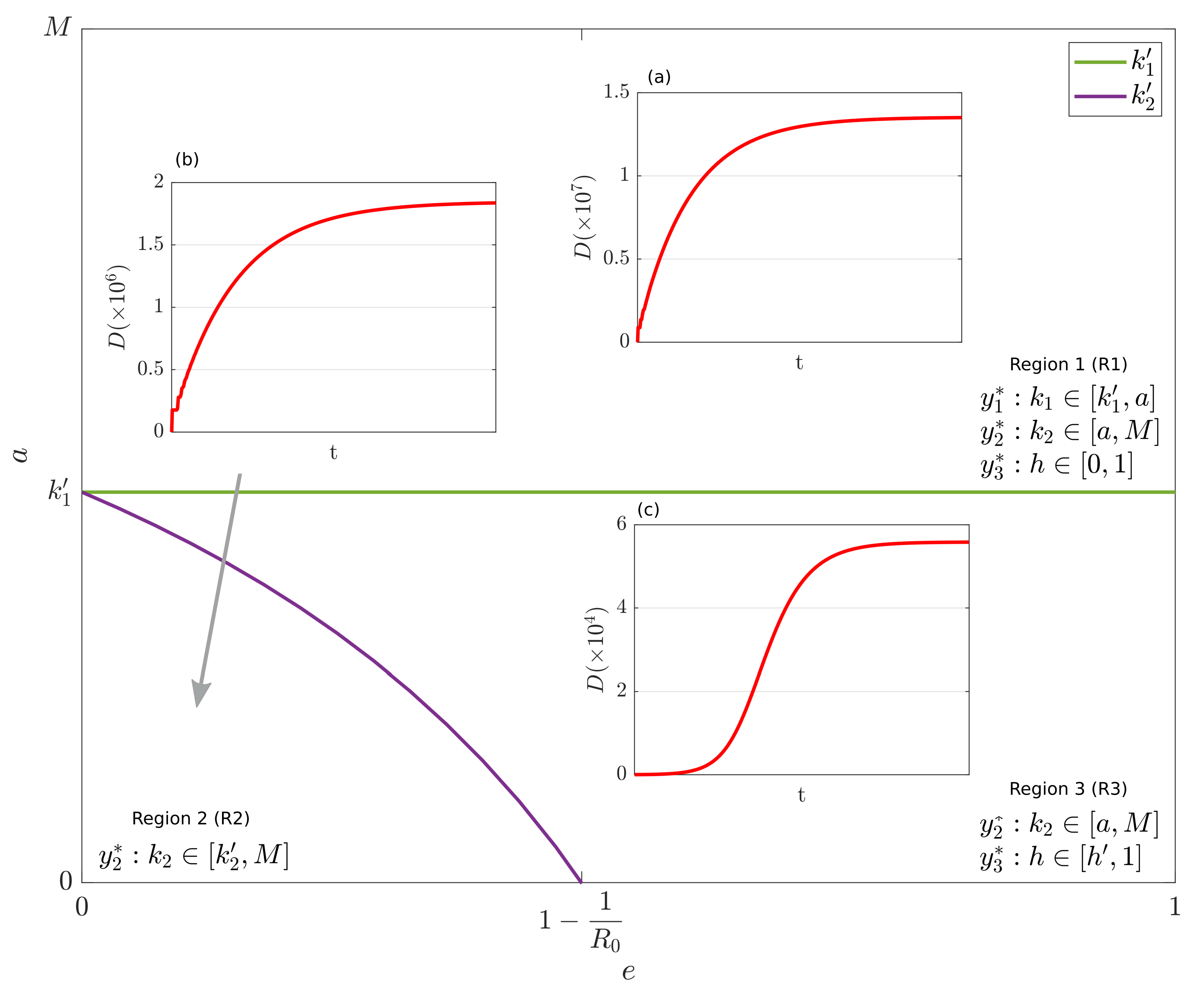
By analyzing the case where ${\mathcal{R}}_0>1$ (i.e., the disease is sufficiently strong to diffuse in the population), we observe that, in agreement to Propositions 1–3, the plane $(e,a)$ is subdivided into three regions: R1 ($a>k_1^{\prime }$), R2 ($k_2^{\prime }<a<k_1^{\prime }$) and R3 ($a<k_1^{\prime }$, $a>k_2^{\prime }$). In R1, $y_1^{*}\left(k_1\right)$ with $k_1\in [k_1^{\prime },a]$, $y_2^{*}\left(k_2\right)$ with $k_2\in [a,M]$ and $y_3^{*}\left(h\right)$ with $h\in [0,1]$ are reachable by different initial conditions. In R2, $y_2^{*}\left(k_2\right)$ with $k_2\in [k_2^{\prime },M]$ are reachable. In R3, $y_2^{*}\left(k_2\right)$ with $k_2\in [a,M]$ and $y_3^{*}\left(h\right)$ with $h\in [h^{\prime },1]$ are reachable. In Figure 2, the three regions are depicted. The insets (a), (b) and (c) depict the dynamics of D for suitable combinations of e and a chosen in R1, R2 and R3, respectively. The values of the parameters are reported in the caption of Figure 2. Noticeably, the asymptotic numbers of dead people in the three regions are significantly different. Specifically, in R3 this number is up to 3 orders of magnitude lower than R1. R2 has an intermediate level. This fact confirms that the proposed IGM model well embodies the underlying containment mechanisms based on the interplay between cooperation, observation and epidemic strength. In particular, region R3 is characterized by low values of a (i.e., high sensitivity of people to the observation on the epidemic status) and enough high values of e (i.e., high weight for the behavioral variable x), thus making it the most desirable.

2.4. Available Data

In this work, we use data collected in Italy by Protezione Civile (the national Italian agency dealing with the prediction, prevention and management of emergency events), updated daily on GitHub [38]. In particular, the data used in this paper correspond to the infected, recovered and dead people per each day in the period of observation from 24 March 2020 to 14 September 2021 (540 days). The initial amount of infected, recovered and dead is taken equal to the initial value of the corresponding variable in the dataset. Since only the sum of the initial conditions of susceptible and undetected infected is known, $U\left(0\right)$ or $S\left(0\right)$ will be estimated and the other one will be calculated by difference from the condition $S\left(0\right)+U\left(0\right)+I\left(0\right)+R\left(0\right)+D\left(0\right)=M$.

2.5. Parameters Estimation

The proposed model is characterized by three different sets of parameters. The first set (${\theta }_1$) includes parameters that are constant for the model but are assumed unknown, and hence they are estimated from data. The unknown initial condition of the effective susceptible individuals $S\left(0\right)$ is also estimated together with the initial condition of the behavioral variable $x\left(0\right)$. The second set (${\theta }_2$) is composed by unknown estimated time-varying parameters, allowing us to take into account the epidemic evolution over time windows of size $T_W=30$ days. Since the dataset is composed of 540 days, there are in total $W=18$ time windows. The last set (${\theta }_3$) consists of parameters fixed according to the literature values, since these are related to specific biological properties of COVID-19.

The estimation problem is formalized as follows:

$${\displaystyle \widehat{\theta }=arg\underset{{\theta }_1,{\theta }_2}{min}\frac{1}{W·T_W}\sum _{j=0}^{W·T_W-1}\sum _{\Xi \in \{I,R,D\}}{\left(\frac{\widehat{\Xi }\left(j\right)-\Xi \left(j\right)}{\widehat{\Xi }\left(j\right)}\right)}^2,}$$

(17)

where $\widehat{I}$, $\widehat{R}$ and $\widehat{D}$ represent the real measurements of infected, recovered and dead individuals, respectively.

The estimation problem (17) has been solved for both IM and IGM. For IM, ${\theta }_1=\left\{S\left(0\right)\right\}$, ${\theta }_2=\{\beta ,\alpha ,\omega ,\zeta \}$ and ${\theta }_3=\{\gamma ,\tau \}=\left\{{\displaystyle \frac{1}{14},0.166}\right\}$, according to [25]. For IGM, ${\theta }_1=\{S\left(0\right),x\left(0\right),{\beta }_0,$${\sigma }_C^0,{\sigma }_N^0\}$, ${\theta }_2=\{\alpha ,\omega ,\zeta ,e,a\}$ and ${\theta }_3$ is the same as in IM. Notice that, since the variable e and x are absent in the IM model, then Equation (9) reduces to:

$$\beta ={\beta }_0,$$

(18)

and ${\beta }_0$ is assumed time varying in the estimation procedure ($\beta ={\beta }_0\in {\theta }_2$). The larger number of parameters of IGM is due to presence of the game dynamics. Additionally, for both IM and IGM, since $S\left(0\right)+U\left(0\right)+I\left(0\right)+R\left(0\right)+D\left(0\right)=M$, then we estimate $S\left(0\right)$, and then calculate $U\left(0\right)=M-S\left(0\right)-I\left(0\right)-R\left(0\right)-D\left(0\right),$ where $I\left(0\right)$, $R\left(0\right)$ and $D\left(0\right)$ are set equal the first values of the dataset, and $M\simeq 6.024\times {10}^7$ indicates the Italian population size.

Furthermore, the time varying parameters in ${\theta }_2$ are estimated for each time window, i.e., we have ${\theta }_{2,1},{\theta }_{2,2},\dots ,{\theta }_{2,W}$.

Suitable constraints for each parameter in ${\theta }_1$ and ${\theta }_2$ have been set to guarantee their physical and/or mathematical meaning. The specific ranges of the parameters, the initial conditions and the estimated values are reported in

Table 1. Values of the estimated parameters in the set ${\theta }_1$ and in the ${\theta }_2$, values of parameters in the set ${\theta }_3$, ranges and initial conditions used for the estimation. Moreover, t.v. stands for “time varying”, while n.a. means that the parameter is not estimated in the corresponding model.

	Range	Param. i.c.	IM est.	IGM est.	Meaning and Definition
${\beta }_0$	$[0.1,0.7]$	$0.5$	t.v.	$0.33$	Natural infection rate. Ref. to Equations (9) and (18) for the relationship between ${\beta }_0$ and $\beta$ in IGM and IM, respectively.
${\sigma }_C^0$	$[0.01,10]$	$4.22$	n.a.	$0.66$	Net game payoff for cooperation. Ref. to Equation (5) for ${\sigma }_C$ in IGM.
${\sigma }_N^0$	$[-10,-0.01]$	$-4.2$	n.a.	$-0.65$	Net game payoff for defection. Ref. to Equation (6) for ${\sigma }_D$ in IGM.
$S\left(0\right)$	$[0.98·M,M]$	$59\times {10}^6$	$6\times {10}^7$	$6\times {10}^7$	Susceptibles initial condition.
$x\left(0\right)$	$[0.1,0.9]$	$0.7$	n.a.	$0.65$	Cooperation initial condition.
e	$[0.05,0.95]$	$0.75$	n.a.	t.v.	Weight of cooperation in $\beta$.
a	$[1,{10}^6]$	$8.7\times {10}^4$	n.a.	t.v.	Sensitivity to disease strength.
$\alpha$	$[{10}^{-4},0.28]$	$0.03$	t.v.	t.v.	Reinfection rate.
$\omega$	$[{10}^{-4},0.14]$	$0.02$	t.v.	t.v.	Recovery rate for detected.
$\zeta$	$[{10}^{-4},0.3]$	$0.01$	t.v.	t.v.	Death rate.
$\gamma$	$1/14$				Recovery rate for undetected.
$\tau$	$0.166$				Detection rate.

in the Section 3. The same constraints are used in both IM and IGM.

The Matlab source code for the estimation and simulation of both IM and IGM described in this work is available at https://github.com/dariomadeo/IGM (created on 20 December 2021).

3. Results

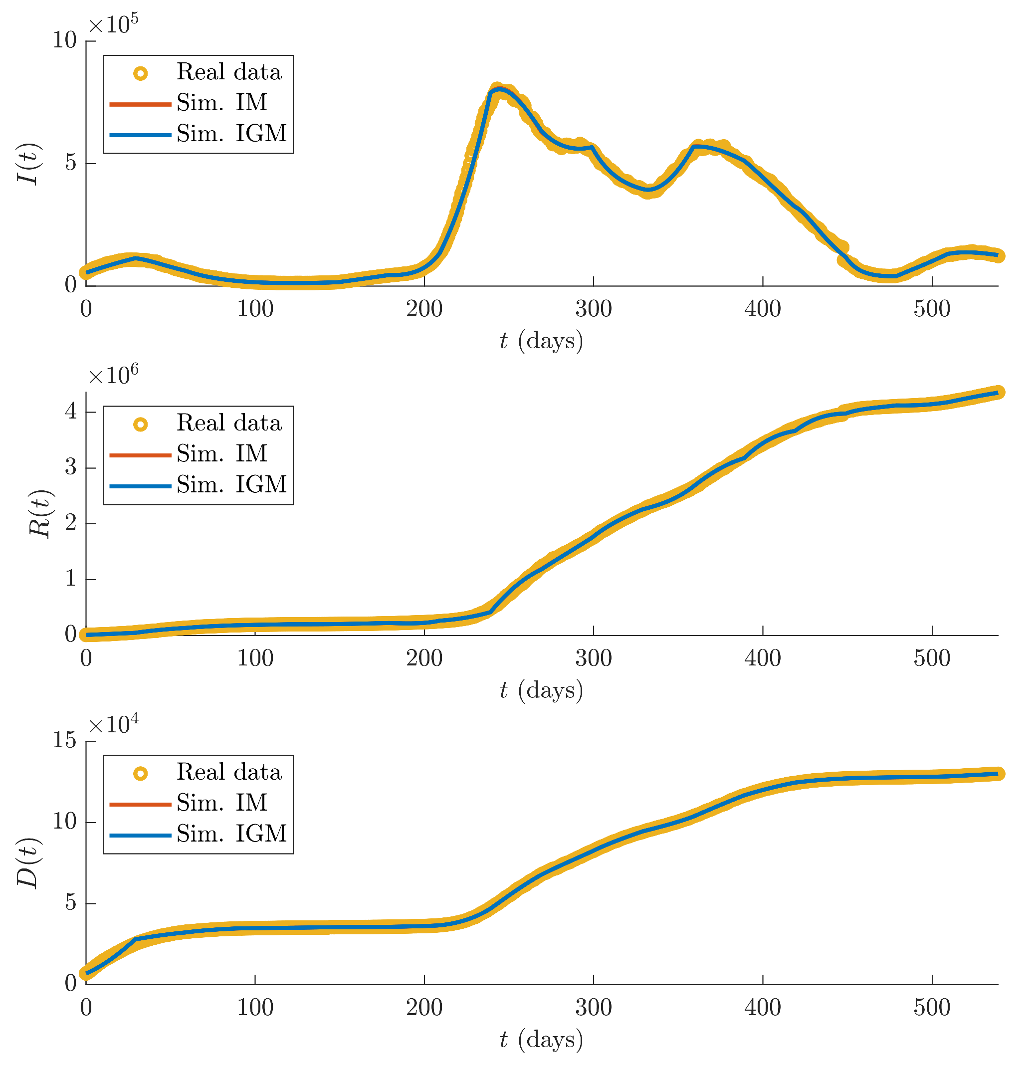
In this Section, the results of the parameter estimation procedure are reported. Figure 3 shows the recorded data $\widehat{I}$, $\widehat{R}$ and $\widehat{D}$ (yellow dots), and the simulations of the three state variables I, R and D of IM (red lines) and IGM (blue lines) obtained using the estimated parameters.

It can be seen that the fitting performances between simulations of both IM and IGM model and real data, evaluated in terms of average percentage errors over times of the three measured state variables, defined as:

$$\mathrm{err}(\Xi )=100·\frac{1}{T}\sum _{t=t_0}^{t_0+T-1}\left|\frac{\widehat{\Xi }\left(t\right)-\Xi \left(t\right)}{\Xi \left(t\right)}\right|,$$

(19)

where $\Xi \in \{I,R,D\}$, are satisfactory (see

Table 2. Fitting results. Percentage errors between data and simulations, averaged over time for both IM and IGM models (see Equation (19)).

	IM	IGM
$\mathrm{err}\left(I\right)$	2.4%	2.3%
$\mathrm{err}\left(R\right)$	7.0%	7.1%
$\mathrm{err}\left(D\right)$	0.2%	0.2%

).

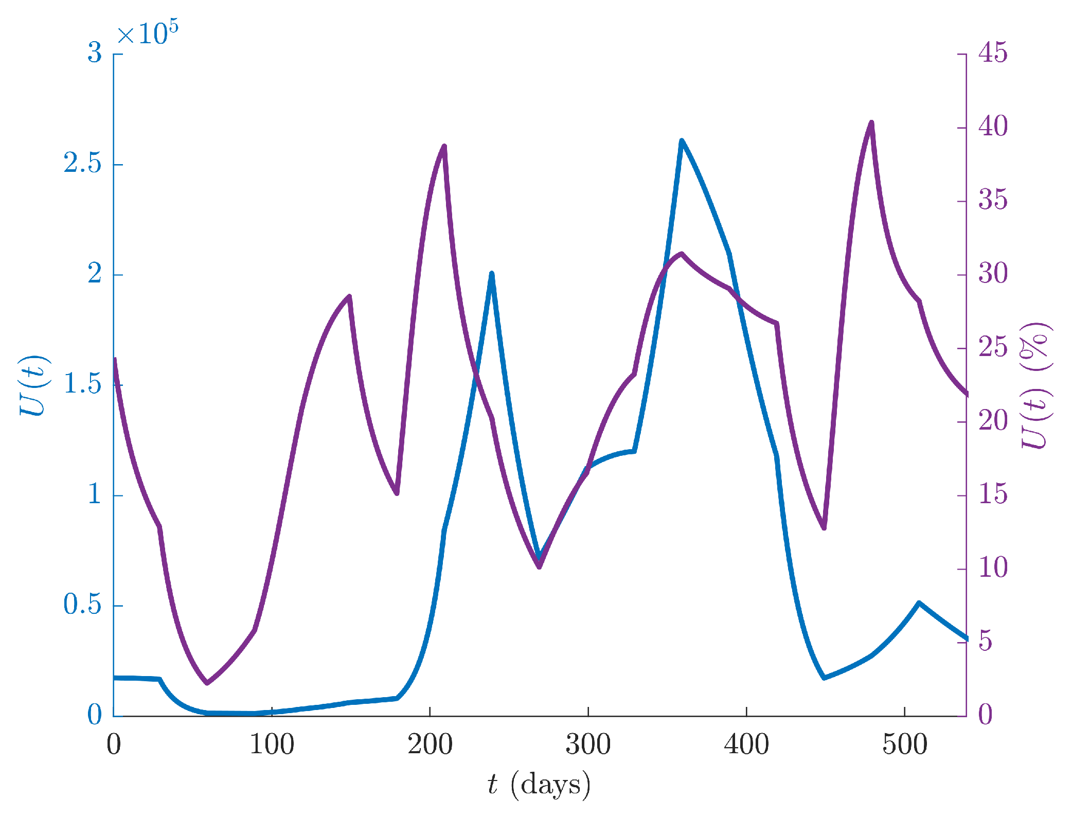
Figure 4 shows the dynamics of the undetected infected individuals U of IGM (blue line, left ordinate scale), as well as the percentage of undetected infected individuals with respect to the total infected population $U+I$ (violet line, right ordinate scale) over the whole time period. The percentage of undetected cases over the total is about $20\%$ in average, with a peak of $40\%$, indicating that the number of unrecorded cases is high, and hence the adoption of more organized containment measures, such as screenings and vaccination campaigns are still desirable to prevent future disease resurgences.

The fixed parameters estimated by solving the optimization problem (17) over $W·T_w=540$ days of recordings of the variables I, R and D, are reported in Table 1, which includes also the list of all the model parameters, constant, fixed, and time varying, and their meaning. The evolution of $\alpha$, $\omega$, and $\zeta$, is drawn in Figure 5, where the red lines are related to IM, while the blue ones to IGM. Subplot (a) contains the dynamics of the reinfection rate $\alpha$. In subplot (b), the time course of the recovery rate $\omega$ is drawn. In subplot (c), the dynamic of the death rate $\zeta$ is depicted, which decreases over time, thanks to the improvement of the caregivers’ techniques and to the vaccination campaign. In all cases, we observe a perfect agreement of the parameter values estimated for the two models.

Furthermore, subplot (a) of Figure 6 shows the dynamics of the control parameter a (blue line), compared with the term $G(I,D)$ (violet line), which rules the game switching. The fluctuations of a over time indicate that this parameter embodies the sensitivity of people to the observation of the pandemic status. High values of a indicate that people are less sensitive to the pandemic status, thus in order to be effectively cooperative they need to know that the number of infected and dead people is very large. The opposite behavior is observed for $G(I,D)$, which embodies the two-sided game. Indeed, people play the Prisoner’s Dilemma game when a is bigger than the pandemic strength, or a Harmony game in the opposite case. In this sense, $G(I,D)$ acts as an “information filter”, balancing the effective information represented by $I+D$ with people perception a of the pandemic. In this regard, it would be interesting to further investigate the quality and effectiveness of the information campaign performed by media and politics. Our results show that, people played Prisoner’s dilemma from March to October 2020, then switched to Harmony game from October 2020 to June 2021 (around day 450), and then again to PD. In this case, the combined effect of spring and successful vaccination campaign reduced the infection entity and allowed people to relax the attention level. Finally, during fall 2021, the game was slightly turning back to Harmony.

Subplot (b) of Figure 6 depicts the time course of the control parameter e (blue line), of the state variable $x\left(t\right)$, corresponding to the average people cooperation (violet) and the combined effect of e and x, which represents the overall efficacy of the containment measures (green line). It is interesting noticing that the overall cooperation is in general increasing from fall 2020 to the end of the observation. This fact embodies a natural “learning process”, leading people to the adoption of good practices even though the government impositions are almost steady. Moreover, recalling the theoretical results depicted in Figure 2, one can see that all estimated values of parameter a fall below $k_1^{\prime }=16.6\times {10}^6$, thus the worst case concerning a potential dramatic number of dead people was avoided along the whole pandemic. For low values of a, the parameter e is most effective in terms of epidemic containment (a deep discussion on this aspect is reported below). Finally, subplot (c) displays the evolution of $\beta$ for IM (red line) and IGM (blue line). The two curves exhibit very similar time courses, meaning that, differently form the usual SIRS models, such as the IM considered in this study, the proposed IGM explains the pandemic trends through new mathematical terms, accounting for the people ability to cooperate with the aim of reducing the infection.

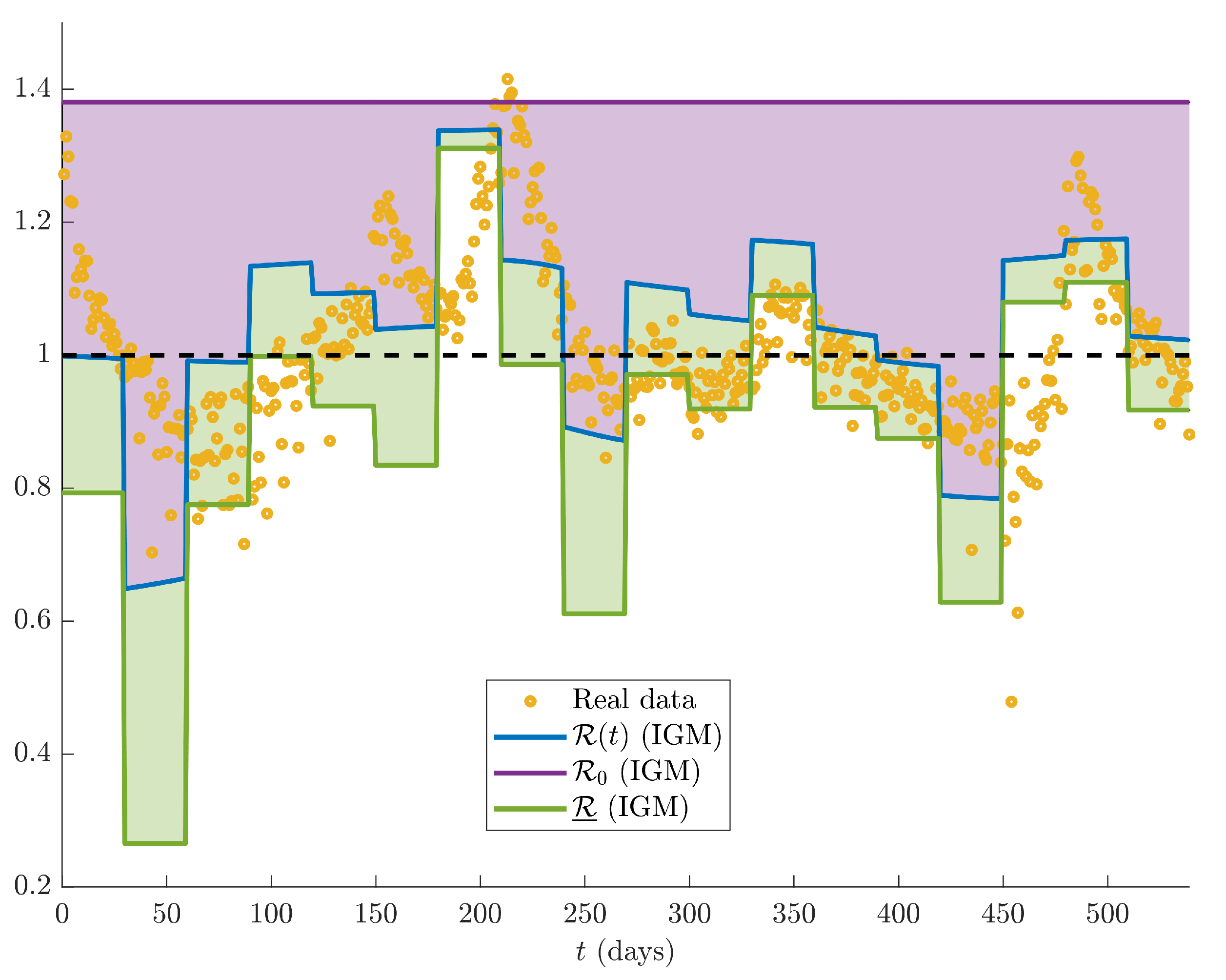
Furthermore, the trend of $\beta$ is coherent with the values of the time varying reproduction number $\mathcal{R}\left(t\right)$, as drawn in Figure 7, where the evolution of $\mathcal{R}\left(t\right)$, evaluated according to different methods, is shown. The reproduction number calculated on real data (yellow circles) according to the following formula [39]:

$$\mathcal{R}\left(t\right)=1+\frac{1}{\gamma +\tau }\frac{I\left(t\right)-I(t-1)}{I(t-1)},$$

where $\gamma =\frac{1}{14}$ and $\tau =0.166$ are assumed constant, according to [25]. We notice that the method implemented for calculating $\mathcal{R}\left(t\right)$ is in agreement with the one that supported the decisions of Italian Government along the whole COVID-19 pandemic [40].

The parameters $\mathcal{R}\left(t\right)$, ${\mathcal{R}}_0$ and $\underline{\mathcal{R}}$ have been also evaluated using Equations (10)–(12), and depicted in Figure 7 with blue, violet and green lines, respectively. According to the theory of dynamical systems, we notice that the trend of $\mathcal{R}\left(t\right)$, evaluated on the basis of the estimated parameters of the IGM, anticipates the $\mathcal{R}\left(t\right)$ calculated using data, thus confirming the good performances of the proposed model. The violet area represents the distance between the current situation (blue line) and the worst case (violet line), i.e., $\mathcal{R}\left(t\right)={\mathcal{R}}_0$, corresponding to the equilibrium state $x=0$. Similarly, the green area corresponds to the distance between the current situation and the best case (green line), i.e., $\mathcal{R}\left(t\right)=\underline{\mathcal{R}}$, corresponding to the equilibrium state $x=1$. Moreover, in order $\underline{\mathcal{R}}$ to be minimum, the parameter e should be as large as possible. Then, at each time window, the best containment of the epidemic spread corresponds to have the blue curve coinciding to the green one, both lower than 1.

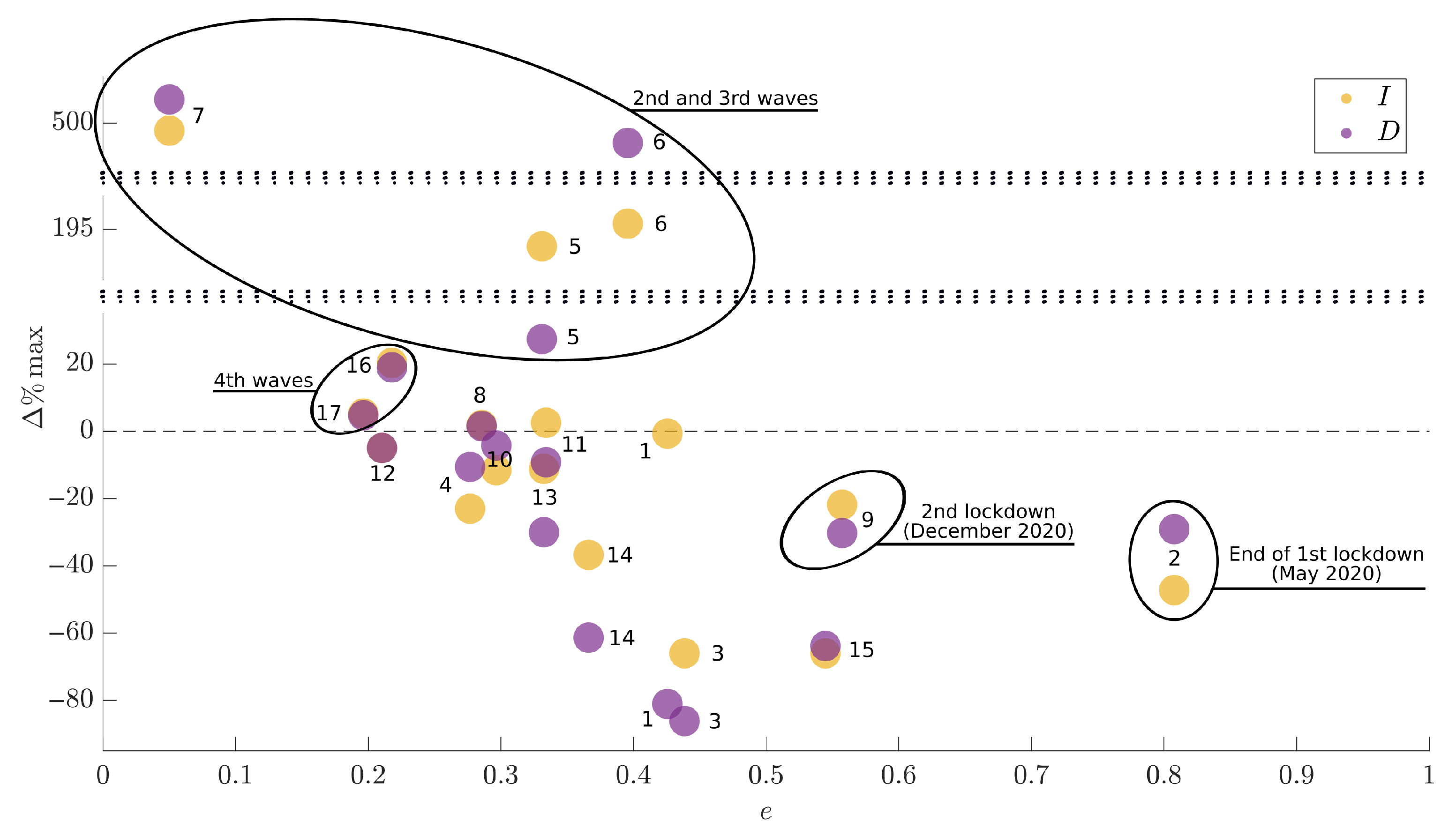
Upon these theoretical considerations, jointly with the very good performances of the proposed model, we can use parameter e to evaluate how successful have been the containment measures. To this aim, Figure 8 depicts the percentage variation over two consecutive months between the maximum values of infected (yellow) and dead (violet) individuals (y-axis), obtained with the value of e (x-axis) set during the first month, as indicated by the label. A visual inspection of the Figure reveals that the best results have been achieved for e sufficiently high (see also Figure 2 as reference), such as during the second lockdown (month 9, November and December 2021). Moreover, at the end of the first lockdown (month 2, May and June 2020) the value of e was very high, coherently to the heavy efforts asked to people in that period. On the other hand, we highlight the fact that the second, third and fourth waves, representing the periods in which the infection reached the highest peaks in both absolute and relative terms, resulted from the use of low values of the parameter e. These results are highlighted by circles in Figure 8, where, for example, the periods indicated by labels 2 and 9 clearly belong to region R3 of Figure 2.

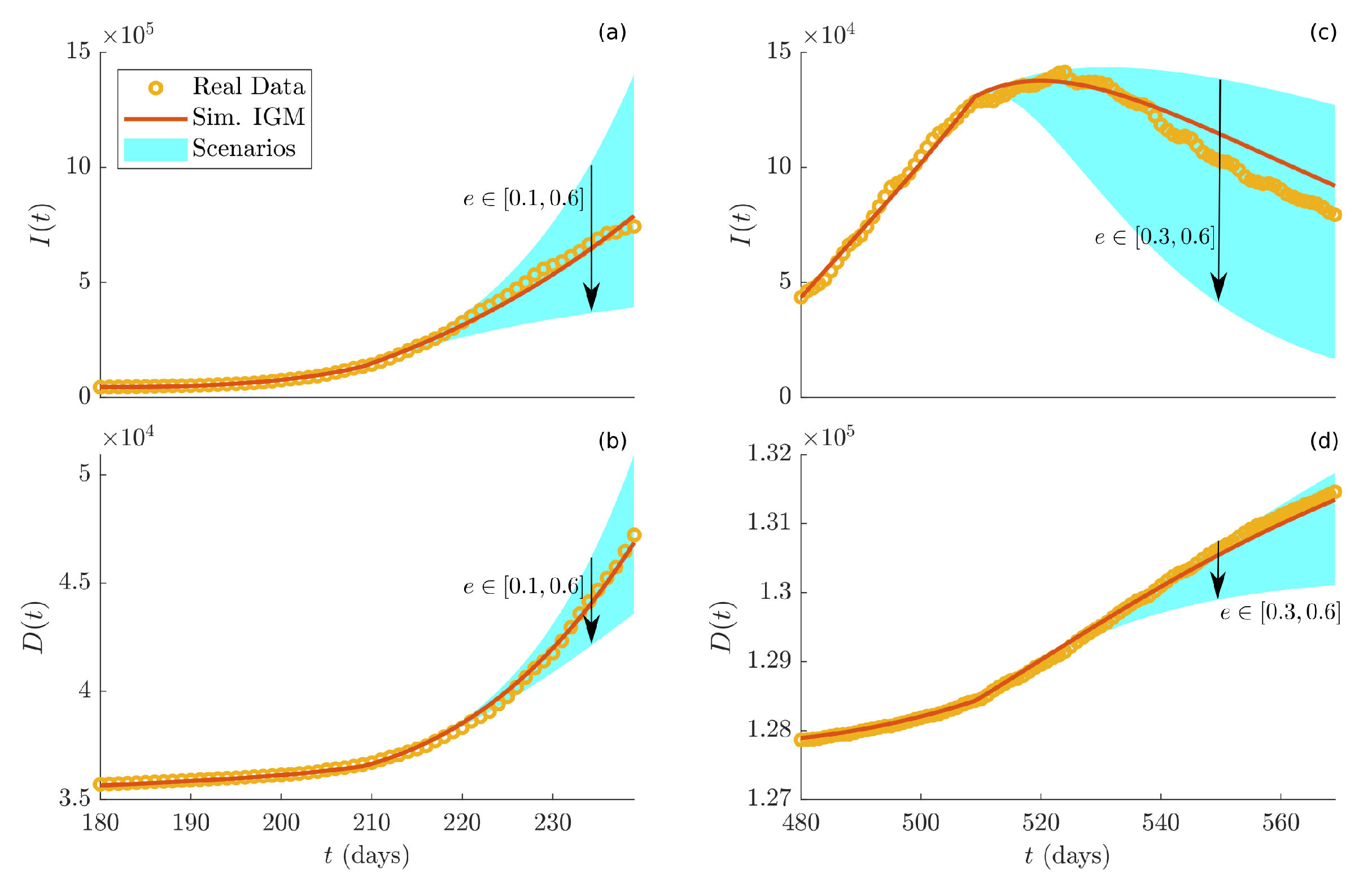
The impact of the control parameter e on the pandemic has been inspected in two different periods. The first period starts on day 210 (beginning of the second wave), and the parameter e is assumed varying in the next time window between $0.1$ and $0.6$, around the estimated value $e=0.29$. Subplots (a) and (b) of Figure 9 display the resulting infected and dead individuals, respectively. The second period starts on day 510, where in the next two time windows, the parameter e varies in the range $[0.3,0.6]$, which includes the value $e=0.34$ estimated in the first window (from day 510 to day 539). Subplots (c) and (d) of Figure 9 show the simulated infected and dead individuals, respectively. In each subplot, yellow dots indicate real data, the red curve is the simulation of the IGM using the estimated parameters, and the light blue area represents the range of variations of the dynamics for different values of e. It is clear that reducing the value of e produces an increase of both infected and dead individuals. On the other hand, when e is fostered, positive effects on the pandemic status are observed. Overall, this analysis suggests that, even though a strong increase of the parameter e can heavily drop the current pandemic status, its values should be chosen in a wise way, in order not to stress too much the population. Indeed, very good results are achievable even by setting e to value significantly lower than its maximum, i.e., $e<1$.

In order to deeply investigate the meaningfulness of the developed model, we recall that the time varying parameters common to IM and IGM, i.e., $\alpha$, $\omega$, $\zeta$ and $\beta$, have similar shapes (see Figure 5 and Figure 6). As a consequence, it is interesting to assess the significance of the specific IGM state variables and parameters, such as x, e and a. To this aim, we report the correlation analysis between these parameters and additional data, available in [38,41], not used for the modeling and identification phases. In particular, we have chosen data related to people’s decisions on vaccination and testing. 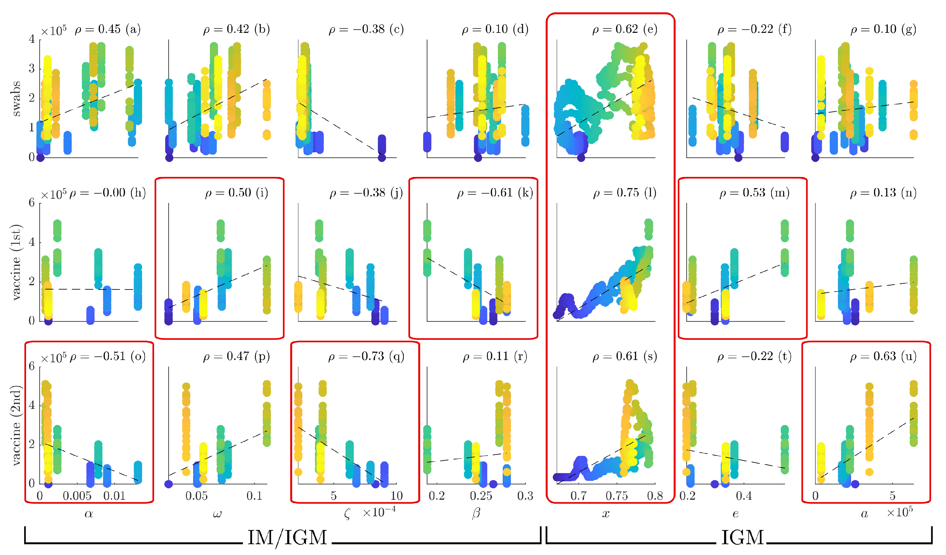Figure 10 reports the scatter plots of the number of daily swabs (subplots (a–g)), first vaccine (subplots (h–n)) and second vaccine (subplots (o–u)) administrations (y-axis) versus $\alpha$, $\omega$, $\zeta$, $\beta$, x, e and a (x-axis).

In the first four columns, the time varying parameters $\alpha$, $\omega$, $\zeta$ and $\beta$ are considered. A correlation of $-0.51$ between the drop infection rate $\alpha$ and the second vaccine administration (subplot (o)), and a correlation of $0.5$ between the recovery rate $\omega$ and the first vaccine administration (subplot (i)) are found. The death rate $\zeta$ has a negative correlation of $-0.73$ with the second vaccine administration (subplot (q)), coherently with the fact that vaccine reduces dramatically the mortality. Finally, the infection rate $\beta$ exhibits, as expected, a negative correlation of $-0.61$ with the first vaccine administration (subplot (k)).

The peculiar structure of the $\beta$ in the IGM (see Equation (9)) allows one to take into account the social dynamics as additional detail, and hence it can be used to better understand the dynamics of vaccination and testing, as well as to plan more appropriate countermeasures. x exhibits high correlations with swabs (subplot (e), $\rho =0.62$), 1st vaccine (subplot (l), $\rho =0.75$) and 2nd vaccine (subplot (s), $\rho =0.61$). Indeed, a strong cooperation implies a diffuse willingness of people to check and protect their own health. Furthermore, significant positive correlations are found between the parameter e and 1st vaccine administration (subplot (m), $\rho =0.53$), and between a and 2nd vaccine administration (subplot (u), $\rho =0.63$). In the fist case, the diffusion of cooperative behavior stimulated an increase of the 1st vaccination in the population. The last case implies that an increased tolerance to the epidemic status may produce a higher propensity to vaccination. These results confirm that the extended IGM is able to shade light on additional aspects related to the social dynamics during the pandemic.

4. Conclusions

This paper presents an extended model, called IGM, which integrates a standard epidemic system and evolutionary games, used to describe the propensity of people and institutions to be cooperative, thus adopting the measures taken to control the epidemic. The resulting model assumes that the infection rate decreases when the cooperation rises, by means of a control parameter e, while the propensity to cooperate is favoured by strong infection levels, ruled by the threshold parameter a, which embodies the awareness of people concerning the gravity of the current sanitary crisis.

A stability analysis of the IGM equilibria was carried out, highlighting the possibility to tune the parameters e and a in order to drive the system dynamics towards regions where the number of potential dead people is dramatically reduced with respect to the non-controlled case. An identification procedure, consisting of the minimization of the relative square difference between real measurements and model simulations to estimate system parameters, has been applied. The results indicate high fitting performances of the developed model. Furthermore, the model, which assumes the presence of a twofold feedback between the infection strength and the propensity of people to comply with the containment measures, turns out to be effective in producing the observed alternating periods of rising and damping of COVID-19 epidemic in Italy. The satisfactory results are also confirmed by the strong correlations found between the behavioral variable x, indicating the cooperation level, and swabs, first and second vaccine administrations.

Overall, thanks to its theoretical properties and to its good performance in terms of fitting, the proposed model aspires to be considered as a reference framework to account simultaneously for the biological aspects of an epidemic and for the social and decision issues related to its containment. Future works will concern the extension of the present model to include the vaccine dynamics, making it even more effective to be adopted by the policy-makers. As a further development, the authors are investigating the impact of “imperfect information” on the described process. Indeed, it is well known that some of the infectious individuals are pauci- or even a-symptomatic. The information provided on the status of the pandemics can be also incorrect due to the difficulties inherent in data collection, or due to the diffusion of fake news. As a natural consequence, it would be interesting to analyze the system behavior by considering only the fraction of (supposedly) known infectious individuals.